Seismology - daveboorew.daveboore.com/pubs_online/bommer_boore_seismology... · 2012-06-25 · ing...

See Also

Analytical Methods: Gravity. Engineering Geology:Seismology; Natural and Anthropogenic Geohazards;

Site and Ground Investigation; Site Classification. Mili-tary Geology. Rock Mechanics. Seismic Surveys. SoilMechanics.

Further Reading

Environmental and Engineering Geophysical Society. http://www.eegs.org/whatis/

Health and Safety Executive (UK) (2000) Avoiding Dangerfrom Underground Services. Health and SafetyExecutive, London.

McCann DM, Eddleston M, Fenning PJ, and Reeves GM(eds.) (1997) Modern Geophysics in Engineering

Geology. Engineering Geology Special Publication 12.London: Geological Society.

McDowell PW, Barker RD, and Butcher AP (eds.)(2002) Geophysics in Engineering Investigations.Engineering Geology Special Publication 19. London:CIRIA.

Milsom J (2003) Field Geophysics, 3rd edn., The Geo-logical Field Guide Series. Chichester: John Wiley &Sons.

Reynolds JM (1997) An Introduction to Applied andEnvironmental Geophysics. Chichester: John Wiley &Sons.

Telford WM, Geldart LP, and Sheriff RE (1990) AppliedGeophysics, 2nd edn. Cambridge: Cambridge UniversityPress.

Zeltica. Geophysical Method Descriptons. http://www.geophysics.co.uk/methods.html

ENGINEERING GEOLOGY/Seismology 499

Seismology

J J Bommer, Imperial College London, London, UK

D M Boore, United States Geological Survey, Menlo

Park, CA, USA

� 2005, Elsevier Ltd. All Rights Reserved.

Introduction

Engineering seismology is an integral part of earth-quake engineering, a specialized branch of civil en-gineering concerned with the protection of the builtenvironment against the potentially destructive effectsof earthquakes. The objective of earthquake engineer-ing can be stated as the reduction or mitigation ofseismic risk, which is understood as the possibility oflosses – human, social or economic – being caused byearthquakes. Seismic risk exists because of the convo-lution of three factors: seismic hazard, exposure, andvulnerability. Seismic hazard refers to the effects ofearthquakes that can cause damage in the built envir-onment, such as the primary effects of ground shakingor ground rupture or secondary effects such as soilliquefaction or landslides. Exposure refers to the pop-ulation, buildings, installations, and infrastructure en-countered at the location where earthquake effectscould occur. Vulnerability represents the likelihoodof damage being sustained by a structure when it isexposed to a particular earthquake effect.

Earthquake Hazards andSeismic Risk

Risk can be reduced in two main ways, the first beingto avoid exposure where seismic hazard is high.

However, human settlement, the construction ofindustrial facilities, and the routing of lifelines suchas roads, bridges, pipelines, telecommunications, andenergy distribution systems are often governed byother factors that are of greater importance. Indeed,for lifelines, which may have total lengths of hun-dreds of kilometres, it will often be impossible toavoid seismic hazards by relocation. Millions ofpeople are living in areas of the world where there isappreciable seismic hazard. The key to mitigatingseismic risk therefore lies in control of vulnerabilityin the built environment, by designing and buildingstructures and facilities with sufficient resistanceto withstand the effects of earthquakes; this is theessence of earthquake engineering.

This is not to say, however, that the aim is toconstruct an earthquake-proof built environmentthat will suffer no damage in the case of a strongearthquake. The cost of such levels of protectionwould be extremely high, and, moreover, it mightmean protecting the built environment against eventsthat may not occur within the useful life of a particu-lar building. It is generally not possible to justify suchinvestments, especially when there are many compet-ing demands on resources. Objectives of earthquake-resistant design are often stated in terms that relatedifferent performance objectives to different levels ofearthquake motion, such as no damage being sus-tained due to mild levels of shaking that may occurfrequently, damage being limited to non-structuralelements or to easily repairable levels in struc-tural elements in moderate shaking that occurs occa-sionally, and collapse being avoided under severe

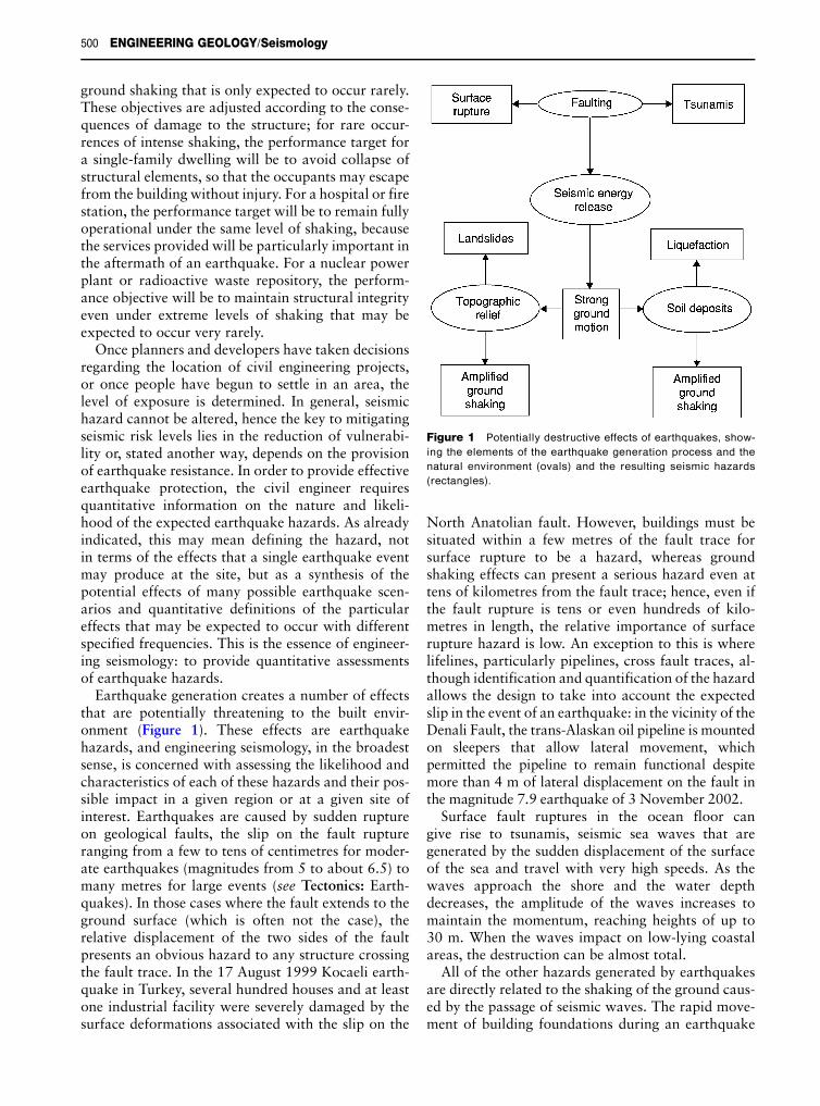
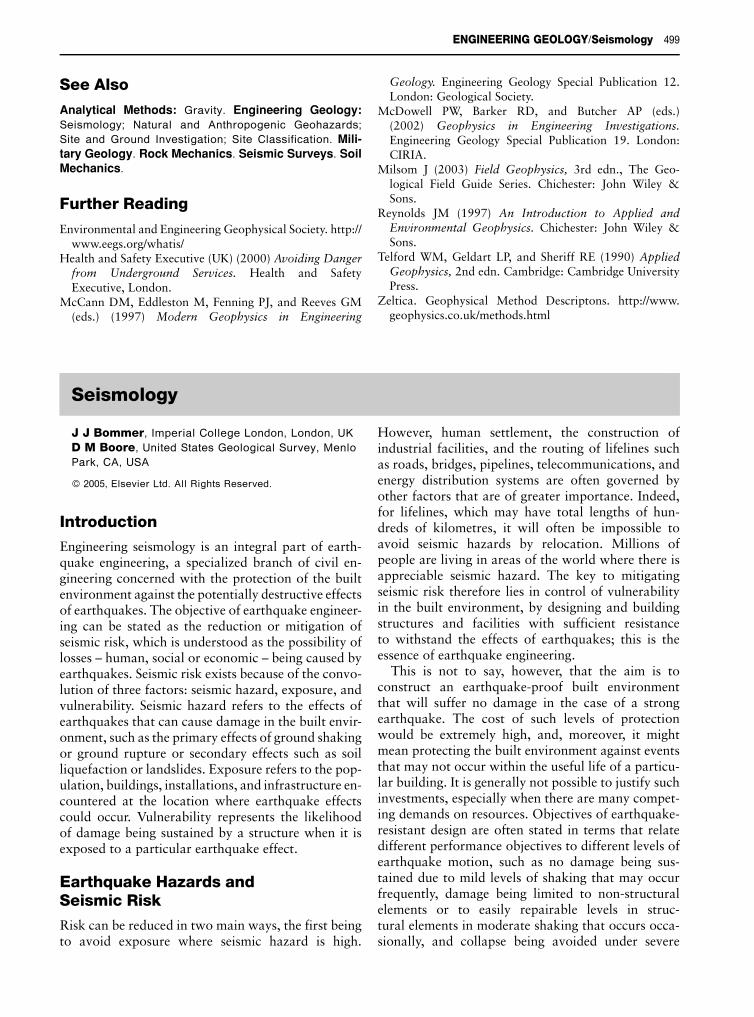
Figure 1 Potentially destructive effects of earthquakes, show-

ing the elements of the earthquake generation process and the

natural environment (ovals) and the resulting seismic hazards

(rectangles).

500 ENGINEERING GEOLOGY/Seismology

ground shaking that is only expected to occur rarely.These objectives are adjusted according to the conse-quences of damage to the structure; for rare occur-rences of intense shaking, the performance target fora single-family dwelling will be to avoid collapse ofstructural elements, so that the occupants may escapefrom the building without injury. For a hospital or firestation, the performance target will be to remain fullyoperational under the same level of shaking, becausethe services provided will be particularly important inthe aftermath of an earthquake. For a nuclear powerplant or radioactive waste repository, the perform-ance objective will be to maintain structural integrityeven under extreme levels of shaking that may beexpected to occur very rarely.

Once planners and developers have taken decisionsregarding the location of civil engineering projects,or once people have begun to settle in an area, thelevel of exposure is determined. In general, seismichazard cannot be altered, hence the key to mitigatingseismic risk levels lies in the reduction of vulnerabi-lity or, stated another way, depends on the provisionof earthquake resistance. In order to provide effectiveearthquake protection, the civil engineer requiresquantitative information on the nature and likeli-hood of the expected earthquake hazards. As alreadyindicated, this may mean defining the hazard, notin terms of the effects that a single earthquake eventmay produce at the site, but as a synthesis of thepotential effects of many possible earthquake scen-arios and quantitative definitions of the particulareffects that may be expected to occur with differentspecified frequencies. This is the essence of engineer-ing seismology: to provide quantitative assessmentsof earthquake hazards.

Earthquake generation creates a number of effectsthat are potentially threatening to the built envir-onment (Figure 1). These effects are earthquakehazards, and engineering seismology, in the broadestsense, is concerned with assessing the likelihood andcharacteristics of each of these hazards and their pos-sible impact in a given region or at a given site ofinterest. Earthquakes are caused by sudden ruptureon geological faults, the slip on the fault ruptureranging from a few to tens of centimetres for moder-ate earthquakes (magnitudes from 5 to about 6.5) tomany metres for large events (see Tectonics: Earth-quakes). In those cases where the fault extends to theground surface (which is often not the case), therelative displacement of the two sides of the faultpresents an obvious hazard to any structure crossingthe fault trace. In the 17 August 1999 Kocaeli earth-quake in Turkey, several hundred houses and at leastone industrial facility were severely damaged by thesurface deformations associated with the slip on the

North Anatolian fault. However, buildings must besituated within a few metres of the fault trace forsurface rupture to be a hazard, whereas groundshaking effects can present a serious hazard even attens of kilometres from the fault trace; hence, even ifthe fault rupture is tens or even hundreds of kilo-metres in length, the relative importance of surfacerupture hazard is low. An exception to this is wherelifelines, particularly pipelines, cross fault traces, al-though identification and quantification of the hazardallows the design to take into account the expectedslip in the event of an earthquake: in the vicinity of theDenali Fault, the trans-Alaskan oil pipeline is mountedon sleepers that allow lateral movement, whichpermitted the pipeline to remain functional despitemore than 4 m of lateral displacement on the fault inthe magnitude 7.9 earthquake of 3 November 2002.

Surface fault ruptures in the ocean floor cangive rise to tsunamis, seismic sea waves that aregenerated by the sudden displacement of the surfaceof the sea and travel with very high speeds. As thewaves approach the shore and the water depthdecreases, the amplitude of the waves increases tomaintain the momentum, reaching heights of up to30 m. When the waves impact on low-lying coastalareas, the destruction can be almost total.

All of the other hazards generated by earthquakesare directly related to the shaking of the ground caus-ed by the passage of seismic waves. The rapid move-ment of building foundations during an earthquake


generates inertial loads that can lead to damage andcollapse, which is the cause of the vast majority offatalities due to earthquakes. For this reason, themain focus of engineering seismology, and also ofthis article, is the assessment of the hazard of groundshaking. Earthquake ground motion can be amplifiedby features of the natural environment, increasingthe hazard to the built environment. Topographicfeatures such as ridges can cause amplification ofthe shaking, and soft soil deposits also tend to in-crease the amplitude of the shaking with respect torock sites. At the same time, the shaking can inducesecondary geotechnical hazards by causing failure ofthe ground. In mountainous or hilly areas, earth-quakes frequently trigger landslides, which cansignificantly compound the losses: the 6 March1987 earthquake in Ecuador triggered landslidesthat interrupted a 40-km segment of the pipelinecarrying oil from the production fields in the Amazonbasin to the coast, thereby cutting one of the majorexports of the country; the earthquake that struck ElSalvador on 13 January 2001 killed about 850people, and nearly all of them were buried bylandslides. In areas where saturated sandy soils areencountered, the ground shaking can induce lique-faction (see Engineering Geology: Liquefaction)through the generation of high pore-water pressures,leading to reduced effective stress and a significantloss of shear strength, which in turns leads to thesinking of buildings into the ground and lateralspreading on river banks and along coasts. Extensivedamage in the 17 January 1994 Kobe earthquake wascaused by liquefaction of reclaimed land, leavingJapan’s second port out of operation for 3 years.

The assessment of landslide and liquefactionhazard involves evaluating the susceptibility of slopesand soil deposits, and determining the expected levelof earthquake ground motion. The basis for earth-quake-resistant design of buildings and bridges alsorequires quantitative assessment of the groundmotion that may be expected at the location of theproject during its design life. Seismic hazard assess-ment in terms of strong ground motion is the activitythat defines engineering seismology.

Measuring EarthquakeGround Motion

The measurement of seismic waves is fundamental toseismology. Earthquake locations and magnitudes aredetermined from recordings on sensitive instruments(called seismographs) installed throughout the world,detecting imperceptible motions of waves generatedby events occurring hundreds or even thousands ofkilometres away. Engineering seismology deals with

ground motions sufficiently close to the causativerupture to be strong enough to present a threat toengineering structures. There are cases in whichdestructive motions have occurred at significant dis-tances from the earthquake source, generally as theresult of amplification of the motions by very soft soildeposits, such as in the San Francisco Marina Districtduring the 18 October 1989 Loma Prieta earthquake,and even more spectacularly in Mexico City during the19 September 1985 Michoacan earthquake, almost400 km from the earthquake source. In general, how-ever, the realm of interest of engineering seismology islimited to a few tens of kilometres from the earthquakesource, perhaps extending to 100 km or a little morefor the largest magnitude events.

Seismographs specifically designed for measuringthe strong ground motion near the source of an earth-quake are called accelerographs, and the records thatthey produce are accelerograms. The first accelero-graphs were installed in California in 1932, almostfour decades after the first seismographs, the delaybeing caused by the challenge of constructing instru-ments that were simultaneously sensitive enough toproduce accurate records of the ground accelerationwhile being of sufficient robustness to withstand theshaking without damage.

Prior to the development of the first accelero-graphs, the only way to quantify earthquake shakingwas through the use of intensity scales, which providean index reflecting the strength of ground shaking at aparticular location during an earthquake. The indexis evaluated on the basis of observations of howpeople, objects, and buildings respond to the shaking(Table 1). Some intensity scales also include the re-sponse of the ground with indicators such as slump-ing, ground cracking, and landslides, but thesephenomena are generally considered to be dependenton too many variables to be reliable indicators ofthe strength of ground shaking. At the lower intensitydegrees, the most important indicators are related tohuman perception of the shaking, whereas at thehigher levels, the assessment is based primarily onthe damage sustained by different classes of buildings.A common misconception is that intensity is a meas-ure of damage, whereas it is in fact a measure of thestrength of ground motion inferred from buildingdamage, whence a single intensity degree can corres-pond to severe damage in vulnerable rural dwellingsand minor damage in engineered constructions. Themost widely used intensity scales, both of which have12 degrees and which are broadly equivalent, are theModified Mercalli (MM), used in the Americas, andthe 1998 European Macroseismic Scale (EMS-98),which has replaced the Medvedev–Sponheuer–Karnik(MSK) scale.

Table 1 Summary of the 1998 European Macroseismic Scale

Intensity Definition Effects on people and buildingsa

I Not felt Not felt; detected only by sensitive instruments

II Scarcely felt Felt by very few people, mainly those who are in particularly favourable conditions at rest

and indoors

III Weak Felt by a few people, mostly those at rest

IV Largely observed Felt by many people indoors and very few outdoors; a few people are awakened by the shaking

V Strong Felt by most people indoors and a few outdoors; a few people are frightened and many who are

sleeping are awakened by the shaking

Fine cracks in a few of the most vulnerable types of buildings, such as adobe and unreinforced

masonry

VI Slightly damaging Shaking felt by nearly everyone indoors and by many outdoors; a few people lose their balance

Minor cracks in many vulnerable buildings and in a few poor-quality RC structures; a few of the

most vulnerable buildings have cracks in walls and spalling of fairly large pieces of plaster

VII Damaging Most people are frightened by the shaking, and many have difficulty standing, especially those on

upper storeys of buildings

Many adobe and unreinforced masonry buildings sustain large cracks and damage to roofs and

chimneys; some will have serious failures in walls and partial collapse of roofs and floors;

minor cracks in RC structures with some earthquake-resistant design, more significant cracks

in poor-quality RC structures

VIII Heavily damaged Many find it difficult to stand

Many vulnerable buildings experience partial collapse and some collapse completely; large and

extensive cracks in poor-quality RC buildings and many cracks in RC buildings with some

degree of earthquake-resistant design

IX Destructive General panic (this is the highest degree of intensity that can be assessed from human response)

General and extensive damage in vulnerable buildings; cracks in columns, beams, and partition

walls of RC buildings, with some of those of poor quality suffering heavy structural damage and

partial collapse; non-structural damage in RC structures with high level of earthquake-resistant

design

X Very destructive Partial or total collapse in nearly all vulnerable buildings; extensive structural damage in RC and

steel structures

XI Devastating Extensive damage and widespread collapse in nearly all building types; very rarely observed,

if ever

XII Completely

devastating

Cataclysmic damage; has never been observed and is probably not physically realizable

a RC, Reinforced concrete.


A very useful picture of the strength and distribu-tion of ground shaking in an earthquake can beobtained by mapping intensity observations. Themodal value is assigned to each given location, suchas a village, from all the individual point observationsgathered, and then lines called isoseismals are drawnto enclose areas where the intensity reached the samedegree (Figure 2). Such isoseismal maps have manyapplications, one of the most important of which is toestablish correlations between earthquake size (mag-nitude) and the area enclosed by isoseismals. Theseempirical relations can then be used to estimate themagnitude of historical earthquakes that occurredbefore the advent of the global seismograph networkat the end of nineteenth century, but for which it ispossible to compile isoseismal maps from writtenaccounts of the earthquake effects. For engineeringdesign and analysis, however, intensity values are oflimited use because they cannot be reliably translatedinto numerical values related to the acceleration ordisplacement of the ground. Indeed, intensities areusually expressed in Roman numerals precisely to

reinforce the idea that they are broad indices ratherthan numerical measurements. This is why accelero-grams are invaluable to earthquake engineering, pro-viding detailed measurements of the actual movementof the ground during strong earthquake-inducedshaking.

Accelerograms generally consist of three mutuallyperpendicular components of motion, two horizontaland one vertical, registering the ground accelerationagainst time (Figure 3). The first generation of accel-erographs produced analogue records on paper orfilm, which had to be digitized in order to be able toperform numerical analyses. The analogue recordingand the digitization process both introduce noise intothe signal; this noise then requires processing of thetime-series to improve the signal-to-noise ratio, par-ticularly at long periods. This processing generallyinvolves the application of digital filters. The currentmodels of accelerographs record digitally, thus by-passing the time-consuming and troublesome processof digitization, and producing records with muchlower noise contamination. Another advantage of

Figure 2 (A) Regional isoseismal map of the Lisbon earthquake of January 1531. (B) Isoseismal map for the epicentral area of the Lisbon earthquake of January 1531, superimposed on a

map of the local geology. Reprinted with permission from Justo JL and Salwa C (1998) The 1531 Lisbon earthquake. Bulletin of the Seismological Society of America 88(2): 319–328.

� Seismological Society of America.

EN

GIN

EE

RIN

GG

EO

LO

GY

/Seism

olo

gy

503

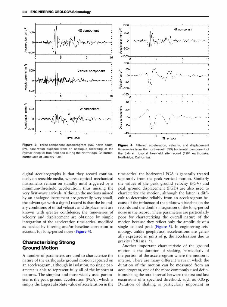
Figure 3 Three-component accelerogram (NS, north–south;

EW, east–west) digitized from an analogue recording at the

Sylmar Hospital free-field site during the Northridge, California,

earthquake of January 1994.

Figure 4 Filtered acceleration, velocity, and displacement

time-series from the north–south (NS) horizontal component of

the Sylmar Hospital free-field site record (1994 earthquake,

Northridge, California).


digital accelerographs is that they record continu-ously on reusable media, whereas optical–mechanicalinstruments remain on standby until triggered by aminimum-threshold acceleration, thus missing thevery first-wave arrivals. Although the motions missedby an analogue instrument are generally very small,the advantage with a digital record is that the bound-ary conditions of initial velocity and displacement areknown with greater confidence; the time-series ofvelocity and displacement are obtained by simpleintegration of the acceleration time-series, modifiedas needed by filtering and/or baseline correction toaccount for long-period noise (Figure 4).

Characterizing StrongGround Motion

A number of parameters are used to characterize thenature of the earthquake ground motion captured onan accelerogram, although in isolation, no single par-ameter is able to represent fully all of the importantfeatures. The simplest and most widely used param-eter is the peak ground acceleration (PGA), which issimply the largest absolute value of acceleration in the

time-series; the horizontal PGA is generally treatedseparately from the peak vertical motion. Similarlythe values of the peak ground velocity (PGV) andpeak ground displacement (PGD) are also used tocharacterize the motion, although the latter is diffi-cult to determine reliably from an accelerogram be-cause of the influence of the unknown baseline on therecords and the double integration of the long-periodnoise in the record. These parameters are particularlypoor for characterizing the overall nature of themotion because they reflect only the amplitude of asingle isolated peak (Figure 5). In engineering seis-mology, unlike geophysics, accelerations are gener-ally expressed in units of g, the acceleration due togravity (9.81 m s�2).

Another important characteristic of the groundmotion is the duration of shaking, particularly ofthe portion of the accelerogram where the motion isintense. There are many different ways in which theduration of the motion can be measured from anaccelerogram, one of the more commonly used defin-itions being the total interval between the first and lastexcursions of a specified threshold, such as 0.05 g.Duration of shaking is particularly important in

Figure 5 Four horizontal accelerogram components with

nearly the same peak ground acceleration. M, Moment

magnitude; rhyp, distance from the hypocentre.

Figure 6 Husid plots for the four acceleration time-series

shown in Figure 5, showing the build-up of Arias intensity with

time. The upper plot shows the absolute values of Arias intensity;

in the lower plot, the curves are normalized to the maximum

value attained.


the assessment of liquefaction hazard because thebuild-up of pore water pressures is controlled bythe number of cycles of motion as well as by theamplitude of the motion.

A parameter that measures the energy content ofthe ground shaking is the Arias intensity, which isthe integral over time of the square of the acceler-ation. A plot of the build-up of Arias intensity withtime is known as a Husid plot (Figure 6) and it servesto identify the interval over which the majority ofthe energy is imparted. The root-mean-square acc-eleration (arms) is the equivalent constant level ofacceleration over any specified interval of the accel-erogram; the arms is also the square root of the gradi-ent of the Husid plot over the same interval. Ariasintensity has been found to be a useful parameter todefine thresholds of shaking that trigger landslides.

For engineering purposes, the most important re-presentation of earthquake ground motion is the

response spectrum, which is a graph of the maximumresponse experienced by a series of single-degree-of-freedom (SDOF) oscillators when subjected to theacceleration time-series at their bases (Figure 7). Thedynamic characteristics of a SDOF system, such asan idealized inverted pendulum, are fully describedby its natural period of free vibration and itsdamping, usually modelled as an equivalent viscousdamping and expressed as a proportion of the criticaldamping that returns a displaced SDOF system torest without vibrations. In earthquake engineering,the default value generally used is 5% of criticaldamping, the nominal level of damping in a re-inforced concrete structure. The response can bemeasured in terms of the absolute acceleration ofthe mass of the system, or in terms of its velocity ordisplacement relative to the base. The most widelyused spectrum currently is the acceleration response,because the acceleration at the natural period ofthe structure can be multiplied by the mass of thebuilding to estimate the lateral force exerted on thestructure by the earthquake shaking. The naturalperiod of vibration of a building can be very approxi-mately estimated, in seconds, as the number of storeys

Figure 7 Illustration of the concept of the response spectrum. The trace in the lower right-hand corner is the ground acceleration,

and the traces on the left-hand side are the displacement response time-series for simple oscillators with different natural periods of

vibration (Tosc). The maximum displacement of each oscillator is plotted against its natural period to construct the response spectrum

of relative displacement. The lowest two traces in the figure illustrate that for short-period oscillators, the response mimics the ground

acceleration, whereas for long-period oscillators, the response imitates the ground displacement (shown in the upper right-hand

corner). M, Moment magnitude; r, distance to fault rupture.


divided by 10. The acceleration response spectrumintersects the vertical axis at PGA (Figure 8). PGAas a ground-motion parameter has many shortcom-ings, including a very poor correlation with structuraldamage, but one of the main reasons that it is persist-ently used is the fact that it essentially defines theanchor point for the acceleration response spectrum.The relationship between the natural period of vibra-tion of the building and the frequency content ofthe ground motion is a critical factor in determiningthe impact of earthquake shaking on buildings.

In recent years, there has been a gradual tendencyto move away from the use of acceleration res-ponse spectra in force-based seismic design towardsdisplacement-based approaches, because structural

damage is much more closely related to displacementsthan to the forces that are imposed on buildings verybriefly during ground shaking. Techniques for assess-ing the seismic capacity of existing buildings havealready adopted displacement-based approaches,giving rise to greater interest in displacement responsespectra (Figure 9).

Prediction of EarthquakeGround Motion

Recordings of ground motions in previous earth-quakes are used to derive empirical equationsthat may be used to estimate values of particularground-motion parameters for future earthquake

Figure 8 Acceleration response spectra (5% damped) of the four accelerograms shown in Figure 5; the plots are identical except

that the one on the left uses linear axes and the one on the right uses logarithmic axes. Each type of presentation is useful for viewing

particular aspects of the motion, depending on whether the interest is primarily at short or long periods of response. M, Moment

magnitude; rhyp, distance from the hypocentre.

Figure 9 Displacement response spectra of a single accelero-

gram from the 1999 California Hector Mine earthquake (moment

magnitude 7.1; station 596; r = 172 km, r is the distance from the

fault rupture in km, transverse component), plotted for different

levels of damping . The spectra all converge to the value of peak

ground displacement at very long periods.


scenarios. Such empirical equations have been de-rived for a variety of parameters, but the most abun-dant are those for predicting PGA and ordinates ofresponse spectra. The equations are often referred toas attenuation relationships, but this is a misnomerbecause the equations describe both the attenuation(decay) of the amplitudes with distance from theearthquake source and the scaling (increase) of theamplitudes with earthquake magnitude. These two

parameters, earthquake magnitude and source-to-sitedistance, are always included in ground-motion pre-diction equations (Figure 10). The equations aresimple models for a very complex phenomenon andas such there is generally a large amount of scatterabout the fitted curve (Figure 11). The residuals of thelogarithmic values of the observed data points aregenerally found to follow a normal or Gaussian dis-tribution about the mean, and hence the scatter canbe measured by the standard deviation. Predictionsof PGA at the 84-percentile level (i.e., one standarddeviation above the mean value) will generally be asmuch as 80% higher than the median predictions(Figure 12).

The nature of the surface geology can also exert apronounced effect on the recorded ground motion.The presence of soft soil deposits of more than a fewmetres thickness will tend to amplify the groundmotion as the waves propagate from the stiffermaterials below to the surface (Figures 2B and 13).To account for this effect, site classification is gener-ally included as a third explanatory variable in pre-diction equations for response spectrum ordinates,allowing spectra to be predicted for different sites(Figure 14). The modelling of site amplificationeffects in ground-motion prediction equations isgenerally crude, using simple site classificationschemes based on the average shear-wave velocity ofthe upper 30 m at the site and assuming that thedegree of amplification is independent of the ampli-tude of the input motion, whereas it is generally ob-served that weak motion is amplified more thanstrong motion; this non-linear response of soils isreflected only in a few predictive equations. For this

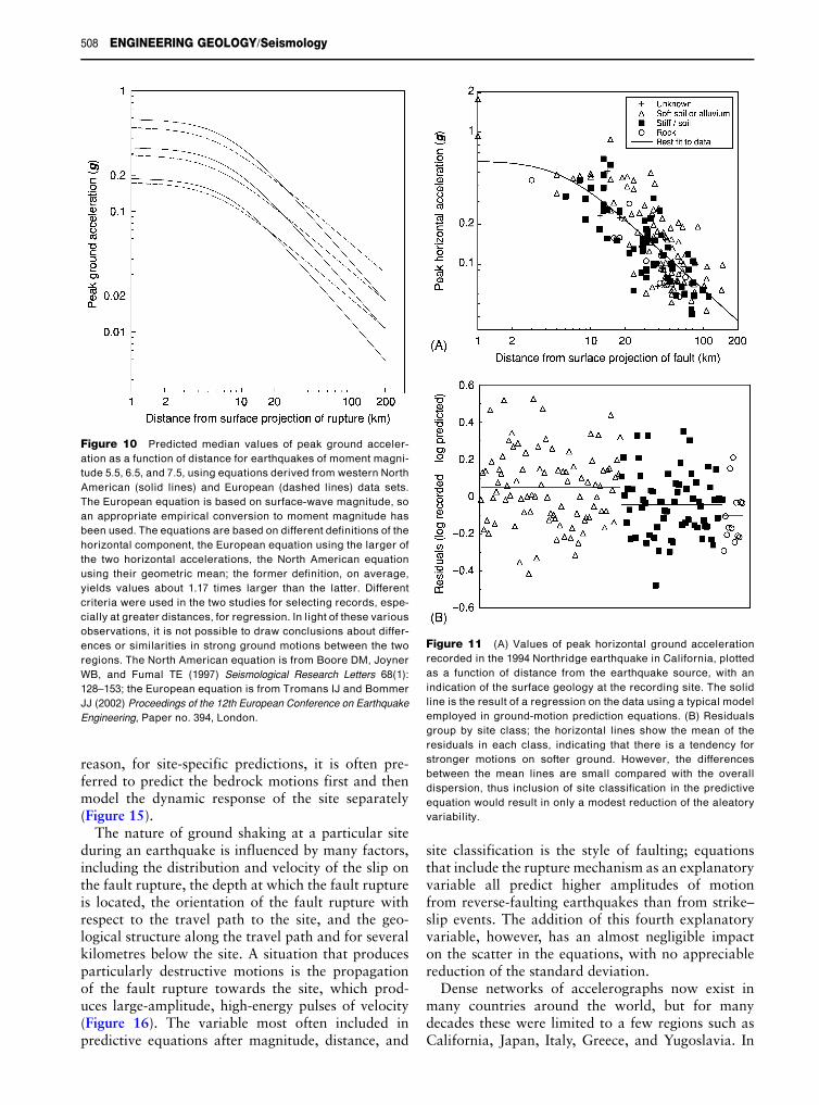
Figure 10 Predicted median values of peak ground acceler-

ation as a function of distance for earthquakes of moment magni-

tude 5.5, 6.5, and 7.5, using equations derived from western North

American (solid lines) and European (dashed lines) data sets.

The European equation is based on surface-wave magnitude, so

an appropriate empirical conversion to moment magnitude has

been used. The equations are based on different definitions of the

horizontal component, the European equation using the larger of

the two horizontal accelerations, the North American equation

using their geometric mean; the former definition, on average,

yields values about 1.17 times larger than the latter. Different

criteria were used in the two studies for selecting records, espe-

cially at greater distances, for regression. In light of these various

observations, it is not possible to draw conclusions about differ-

ences or similarities in strong ground motions between the two

regions. The North American equation is from Boore DM, Joyner

WB, and Fumal TE (1997) Seismological Research Letters 68(1):

128–153; the European equation is from Tromans IJ and Bommer

JJ (2002) Proceedings of the 12th European Conference on Earthquake

Engineering, Paper no. 394, London.

Figure 11 (A) Values of peak horizontal ground acceleration

recorded in the 1994 Northridge earthquake in California, plotted

as a function of distance from the earthquake source, with an

indication of the surface geology at the recording site. The solid

line is the result of a regression on the data using a typical model

employed in ground-motion prediction equations. (B) Residuals

group by site class; the horizontal lines show the mean of the

residuals in each class, indicating that there is a tendency for

stronger motions on softer ground. However, the differences

between the mean lines are small compared with the overall

dispersion, thus inclusion of site classification in the predictive

equation would result in only a modest reduction of the aleatory

variability.


reason, for site-specific predictions, it is often pre-ferred to predict the bedrock motions first and thenmodel the dynamic response of the site separately(Figure 15).

The nature of ground shaking at a particular siteduring an earthquake is influenced by many factors,including the distribution and velocity of the slip onthe fault rupture, the depth at which the fault ruptureis located, the orientation of the fault rupture withrespect to the travel path to the site, and the geo-logical structure along the travel path and for severalkilometres below the site. A situation that producesparticularly destructive motions is the propagationof the fault rupture towards the site, which prod-uces large-amplitude, high-energy pulses of velocity(Figure 16). The variable most often included inpredictive equations after magnitude, distance, and

site classification is the style of faulting; equationsthat include the rupture mechanism as an explanatoryvariable all predict higher amplitudes of motionfrom reverse-faulting earthquakes than from strike–slip events. The addition of this fourth explanatoryvariable, however, has an almost negligible impacton the scatter in the equations, with no appreciablereduction of the standard deviation.

Dense networks of accelerographs now exist inmany countries around the world, but for manydecades these were limited to a few regions such asCalifornia, Japan, Italy, Greece, and Yugoslavia. In

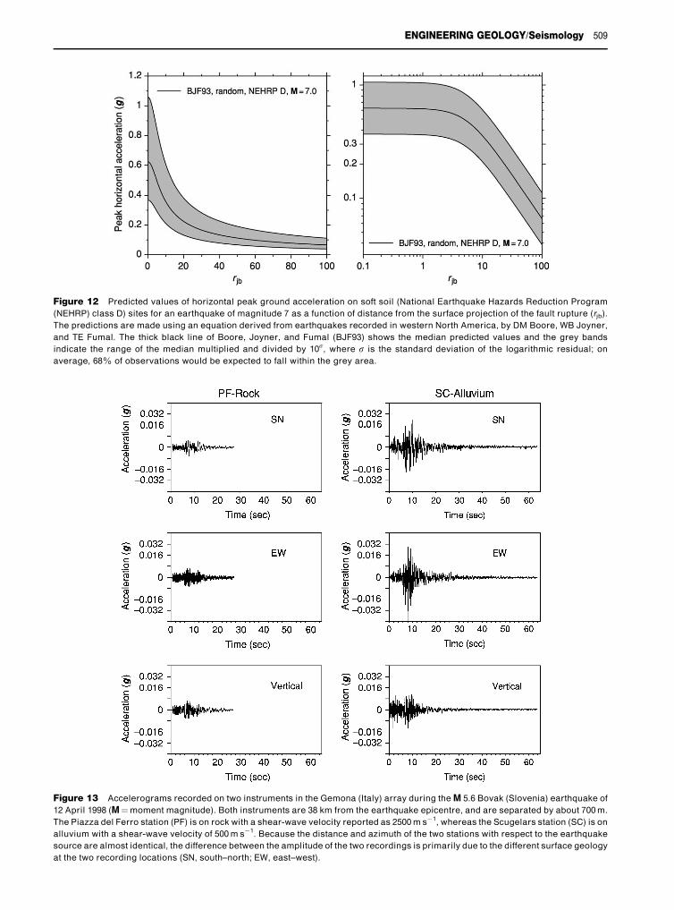
Figure 12 Predicted values of horizontal peak ground acceleration on soft soil (National Earthquake Hazards Reduction Program

(NEHRP) class D) sites for an earthquake of magnitude 7 as a function of distance from the surface projection of the fault rupture (rjb).

The predictions are made using an equation derived from earthquakes recorded in western North America, by DM Boore, WB Joyner,

and TE Fumal. The thick black line of Boore, Joyner, and Fumal (BJF93) shows the median predicted values and the grey bands

indicate the range of the median multiplied and divided by 10s, where s is the standard deviation of the logarithmic residual; on

average, 68% of observations would be expected to fall within the grey area.

Figure 13 Accelerograms recorded on two instruments in the Gemona (Italy) array during the M 5.6 Bovak (Slovenia) earthquake of

12 April 1998 (M¼moment magnitude). Both instruments are 38 km from the earthquake epicentre, and are separated by about 700 m.

The Piazza del Ferro station (PF) is on rock with a shear-wave velocity reported as 2500 m s�1

, whereas the Scugelars station (SC) is on

alluvium with a shear-wave velocity of 500 m s�1

. Because the distance and azimuth of the two stations with respect to the earthquake

source are almost identical, the difference between the amplitude of the two recordings is primarily due to the different surface geology

at the two recording locations (SN, south–north; EW, east–west).


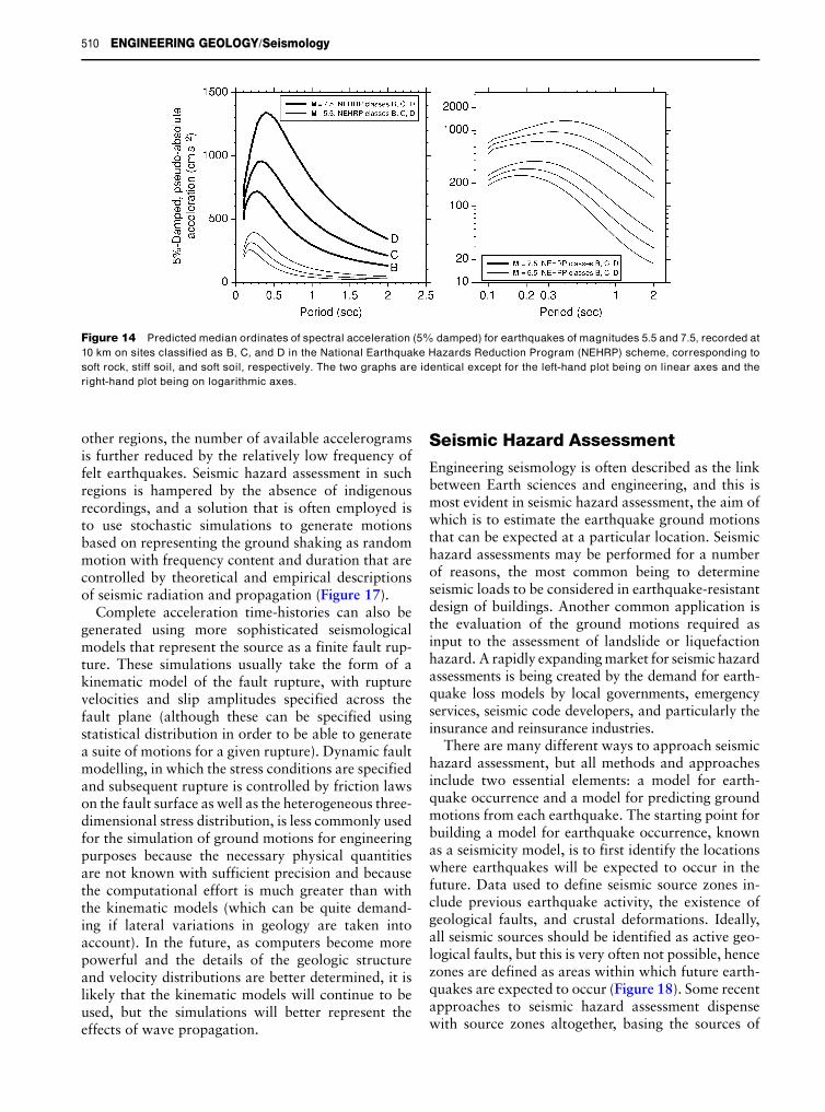
Figure 14 Predicted median ordinates of spectral acceleration (5% damped) for earthquakes of magnitudes 5.5 and 7.5, recorded at

10 km on sites classified as B, C, and D in the National Earthquake Hazards Reduction Program (NEHRP) scheme, corresponding to

soft rock, stiff soil, and soft soil, respectively. The two graphs are identical except for the left-hand plot being on linear axes and the

right-hand plot being on logarithmic axes.


other regions, the number of available accelerogramsis further reduced by the relatively low frequency offelt earthquakes. Seismic hazard assessment in suchregions is hampered by the absence of indigenousrecordings, and a solution that is often employed isto use stochastic simulations to generate motionsbased on representing the ground shaking as randommotion with frequency content and duration that arecontrolled by theoretical and empirical descriptionsof seismic radiation and propagation (Figure 17).

Complete acceleration time-histories can also begenerated using more sophisticated seismologicalmodels that represent the source as a finite fault rup-ture. These simulations usually take the form of akinematic model of the fault rupture, with rupturevelocities and slip amplitudes specified across thefault plane (although these can be specified usingstatistical distribution in order to be able to generatea suite of motions for a given rupture). Dynamic faultmodelling, in which the stress conditions are specifiedand subsequent rupture is controlled by friction lawson the fault surface as well as the heterogeneous three-dimensional stress distribution, is less commonly usedfor the simulation of ground motions for engineeringpurposes because the necessary physical quantitiesare not known with sufficient precision and becausethe computational effort is much greater than withthe kinematic models (which can be quite demand-ing if lateral variations in geology are taken intoaccount). In the future, as computers become morepowerful and the details of the geologic structureand velocity distributions are better determined, it islikely that the kinematic models will continue to beused, but the simulations will better represent theeffects of wave propagation.

Seismic Hazard Assessment

Engineering seismology is often described as the linkbetween Earth sciences and engineering, and this ismost evident in seismic hazard assessment, the aim ofwhich is to estimate the earthquake ground motionsthat can be expected at a particular location. Seismichazard assessments may be performed for a numberof reasons, the most common being to determineseismic loads to be considered in earthquake-resistantdesign of buildings. Another common application isthe evaluation of the ground motions required asinput to the assessment of landslide or liquefactionhazard. A rapidly expanding market for seismic hazardassessments is being created by the demand for earth-quake loss models by local governments, emergencyservices, seismic code developers, and particularly theinsurance and reinsurance industries.

There are many different ways to approach seismichazard assessment, but all methods and approachesinclude two essential elements: a model for earth-quake occurrence and a model for predicting groundmotions from each earthquake. The starting point forbuilding a model for earthquake occurrence, knownas a seismicity model, is to first identify the locationswhere earthquakes will be expected to occur in thefuture. Data used to define seismic source zones in-clude previous earthquake activity, the existence ofgeological faults, and crustal deformations. Ideally,all seismic sources should be identified as active geo-logical faults, but this is very often not possible, hencezones are defined as areas within which future earth-quakes are expected to occur (Figure 18). Some recentapproaches to seismic hazard assessment dispensewith source zones altogether, basing the sources of

Figure 15 Illustration of site response analysis: The input motion in the underlying rock (bottom left) passes through a model of soil

profile to produce the surface motions (top left). The soil characteristics are represented either by the shear-wave velocity or the

shear-wave slowness (right); the slowness is simply the reciprocal of the shear-wave velocity, but there are many reasons for using it

in place of the velocity. The theoretical response of layered systems involves travel times across the layers, which are directly

proportional to the slowness; the proportionality to velocity is inverse. Furthermore, to obtain a representative profile for a soil

class using several boreholes, individual measures of slowness can be directly averaged, whereas it is not correct to do this for

velocities. Finally, the largest influence on the surface motion is due to the differences in velocities near the surface, and these

differences become more clearly apparent when the slowness profile is shown; larger velocity differences in the stiffer layers at

greater depths, which can dominate a velocity profile, are less important.


Figure 16 Velocity time-series obtained from integration of

horizontal accelerograms recorded at Lucerne and Joshua Tree

stations during the 1992 Landers earthquake in California. The

fault rupture propagated towards Lucerne and away from Joshua

Tree, creating forward directivity effects (short-duration shaking

consisting of a concentrated high-energy pulse of motion) at the

former, and backward directivity effects (long-duration shaking of

several small pulses of motion) at the latter. Reprinted with

permission from: Somerville PG, Smith NF, Graves RW, and

Abrahamson NA (1997) Modification of empirical strong ground

motion attenuation relations to include the amplitude and dur-

ation effects of rupture directivity. Seismological Research Letters

68(1): 199–222. � Seismological Society of America.Figure 17 Theoretical Fourier spectra for earthquakes of mag-

nitudes 5 and 7 at 10 km from a rock site, assuming a stress

parameter of 70 bars; f0 is the corner frequency, which is inversely

proportional to the duration of rupture. The lower part of the figure

shows stochastic acceleration time-series generated from these

spectra, from which the influence of magnitude on amplitude and

duration (or number of cycles) can be clearly observed. From

the spectra in the upper part of the figure, it can be appreciated

that scaling with magnitude is frequency-dependent, with larger

magnitude events generating proportionally more long-period

radiation.


postulated future events on past activity. The cata-logue of instrumentally recorded earthquakes extendsback at the very most to 1898, which is a very shortperiod of observation for events for which recurrenceintervals can extend to hundreds or even thousands ofyears. For this reason, great value is to be obtainedfrom extending the catalogue through the carefulinterpretation of historical records, making use ofempirical relationships between magnitude and inten-sity referred to previously. The seismic record can alsobe extended through palaeoseismology, by quantify-ing and dating coseismic displacements on geologicalfaults.

Although the distinction masks many equallymarked differences among the various methods thatfall within each camp, a basic division exists betweendeterministic and probabilistic approaches to seismichazard assessment. In the deterministic approach,only a few earthquake scenarios are considered, andsometimes just one is selected to represent an ap-proximation to the worst case. The controlling earth-quake will generally correspond to an event with thenominal maximum credible magnitude, located at the

location closest to the site within the seismogenicsource; the ground motion is generally calculated asthe 50- or 84-percentile value from the predictionequation. In the probabilistic approach, all possibleearthquake scenarios are considered, includingevents of every magnitude, from the minimum con-sidered to be of engineering significance (�4) up tothe maximum credible, occurring at every possiblelocation within the source zones, and for each magni-tude–distance combination various percentiles ofthe motion are considered to reflect the scatter inthe ground-motion prediction equations. Alternativeoptions for the input parameters may be consideredby using a logic-tree formulation, in which weightsare assigned to different options that reflect the

Figure 18 Seismic sources used for probabilistic hazard study

of the Mississippi embayment. Small squares show the epicen-

tres of earthquakes with the size corresponding to the body-wave

magnitude Mb. (A) The New Madrid seismic source zone repre-

sented as a number of parallel hypothetical faults; (B) the area

sources used to represent seismicity not associated with the

New Madrid zone. Reprinted with permission from Toro GR,

Silva WJ, McGuire RK, and Herrmann RB (1992) Probabilistic

seismic hazard assessment of the Mississippi Embayment. Seis-

mological Research Letters 63(3): 449–475. � Seismological Society

of America.

Figure 19 Logic-tree formulation for probabilistic seismic

hazard study of the Mississippi embayment. For different input

parameters, different options are considered at each node, which

are then assigned weights (p) to reflect the relative confidence in

each option; the values of p at each node always sum to unity. The

source geometry options are the faults shown in Figure 18, and

an alternative model in which the faults are longer. Reprinted

with permission from Toro GR, Silva WJ, McGuire RK, and

Herrmann RB (1992) Probabilistic seismic hazard assessment

of the Mississippi Embayment. Seismological Research Letters

63(3): 449–475. � Seismological Society of America.

Figure 20 Seismic summary hazard curves for spectral accel-

eration at 1-s response period for Memphis (including site re-

sponse), obtained using the logic-tree formulation in Figure 19.

Reprinted with permission from Toro GR, Silva WJ, McGuire RK,

and Herrmann RB (1992) Probabilistic seismic hazard assess-

ment of the Mississippi Embayment. Seismological Research Letters

63(3): 449-475. � Seismological Society of America.


relative confidence in their being the best representa-tion (Figure 19). The output is a ranking of theseearthquake scenarios in terms of the ground-motionamplitudes that they generate at the site and theirfrequency of occurrence (Figure 20).

Seismic hazard assessment can be carried out foran individual site, the output including a responsespectrum calculated ordinate by ordinate, or even a

suite of accelerograms. Hazard assessment is oftenperformed for regions or countries, deriving hazardcurves for a large number of locations and thendrawing contours of a ground-motion parameter(most often PGA) for a given annual frequency ofoccurrence, which is often expressed in terms ofits inverse, known as a return period (Figure 21).Such hazard maps in terms of PGA are the basis of

Figure 21 Contours of spectral accelerations in the Mississippi embayment with a 1000-year return period, for different response

frequencies corresponding to the response periods of 1.0s (top) and 0.1s (middle) and to PGA (botom). The maps show the spectral

accelerations read from the mean hazard curve. Reprinted with permission from Toro GR, Silva WJ, McGuire RK, and Herrmann RB

(1992) Probabilistic seismic hazard assessment of the Mississippi Embayment. Seismological Research Letters 63(3): 449–475. �Seismological Society of America.


ENGINEERING GEOLOGY/Natural and Anthropogenic Geohazards 515

zonation maps included in seismic design codes, fromwhich design response spectra are constructed byanchoring a spectral shape selected for the appropri-ate site class to the PGA value read from the zonationmap.

See Also

Engineering Geology: Aspects of Earthquakes; Nat-

ural and Anthropogenic Geohazards; Liquefaction.

Sedimentary Processes: Particle-Driven Subaqueous

Gravity Processes. Tectonics: Earthquakes; Faults;

Neotectonics.

Further Reading

Abrahamson NA (2000) State of the Practice of SeismicHazard Evaluation. GeoEng 2000, 19–24 November,Melbourne, Australia.

Ambraseys NN (1988) Engineering seismology. EarthquakeEngineering & Structural Dynamics 17: 1–105.

Beskos DE and Anagnostopoulos SA (1997) Computer An-alysis and Design of Earthquake Resistant Structures:A Handbook, chs 3–5. Southampton: ComputationalMechanics Publications.

Bommer JJ (2003) Uncertainty about the uncertainty in seis-mic hazard analysis. Engineering Geology 70: 165–168.

Boore DM (1977) The motion of the ground in earth-quakes. Scientific American 237: 68–78.

Boore DM (2003) Simulation of ground motion using thestochastic method. Pure and Applied Geophysics 160:635–676.

Natural and Anthropogenic Geoh

G J H McCall, Cirencester, Gloucester, UK

� 2005, Elsevier Ltd. All Rights Reserved.

Introduction

The topic of geohazards became popular with scien-tists and the media in the early 1990s at the time of theInternational Decade for Natural Disaster Reductionaimed, by the United Nations, specifically at develop-ing nations in the Third World. It became popularwith the media in the belief that we were movinginto an age of disaster. In particular, the appreciationof the reality of global climate change and human-kind’s contribution in the Industrial Age to globalwarming has led to an awareness of the vulnerabilityof the world in which we live. Geohazards operateat local scales, e.g., in villages and towns, at a regional

Chen W-F and Scawthorn C (2003) Earthquake Engineer-ing Handbook, chs 1–10. Boca Raton, FL: CRC Press.

Douglas J (2003) Earthquake ground motion estimationusing strong-motion records: a review of equations forthe estimation of peak ground acceleration and responsespectral ordinates. Earth Science Reviews 61: 43–104.

Dowrick D (2003) Earthquake Risk Reduction. Chichester,England: John Wiley.

Giardini D (1999) The global seismic hazard assessmentprogram (GSHAP) 1992–1999: summary volume. Annalidi Geofisica 42(6): 957–1230.

Giardini D and Basham P (1993) Technical planningvolume of the ILP’s global seismic hazard assessmentprogram for the UN/IDNDR. Annali di Geofisica36(3/4): 3–257.

Hudson DL (1979) Reading and Interpreting StrongMotion Accelerograms. EERI Monograph, EarthquakeEngineering Research Institute, Oakland, California.

Jackson JA (2001) Living with earthquakes: know yourfaults. Journal of Earthquake Engineering 5(specialissue 1): 5–123.

Kramer SL (1996) Geotechnical Earthquake Engineering.Upper Saddle River, NJ: Prentice-Hall.

Lee WHK, Kanamori H, Jennings PC, and Kisslinger C(2003) International Handbook of Earthquake andEngineering Seismology, Part B. chs. 57–64. Amsterdam:Academic Press.

McGuire RK (2004) Seismic Hazard and Risk Analysis.EERI Monograph MNO-10. Earthquake EngineeringResearch Institute, Oakland, California.

Naeim F (2001) The Seismic Design Handbook, 2nd edn.chs. 1–3. Boston: Kluwer Academic Publ.

Reiter L (1990) Earthquake Hazard Analysis: Issues andInsights. New York: Columbia University Press.

azards

scale, and at the largest scale of all, global. Urbangeohazards represent a specialized and increasinglyimportant type of hazard.

An increasing incidence and scale of risk anddisaster have recently occurred due to a number offactors:

. increased population concentrations;

. increased technological development;

. over-intensive agriculture and increased industrial-ization;

. excessive use of the internal combustion engine andother noxious fume emitters, and wasteful trans-port systems;

. poor technological practices in construction, watermanagement, and waste disposal;

. excessive emphasis on commercial development;

. increased scientific tinkering with Nature withoutdue concern for long-term effects.

Seismology - daveboorew.daveboore.com/pubs_online/bommer_boore_seismology... · 2012-06-25 · ing...

Documents

Transcript of Seismology - daveboorew.daveboore.com/pubs_online/bommer_boore_seismology... · 2012-06-25 · ing...