Processing LA-ICP-MS otolith microchemistry datausing the Fathom Toolbox for Matlab

David L. Jones, PhD

Technical Report ..Laboratory for Otolith Microchemistry

College of Marine ScienceUniversity of South FloridaSt. Petersburg, FL djones@marine.usf.edu

IntroductionThe Fathom Toolbox for Matlab (FTM) is cross-platform collection of custom functionswritten in the Matlab programming language for processing and analyzing oceanographicand multivariate ecological data sets (Jones, ). This open source Toolbox is releasedunder the GNU General Public License (GPL, version .) and is freely available fordownload from: http://www.marine.usf.edu/user/djones. The FTM now includes a suite offunctions in the ‘laser’ folder for processing transient signal data generated by Laser Abla-tion-Inductively Coupled Plasma-Mass Spectrometer (LA-ICP-MS) assays. These func-tions were primarily written to process microchemistry data from assays of fish otoliths,but are readily adaptable to handle LA-ICP-MS data generated from other types of sam-ples as well.

The FTM takes as input the raw time series of analyte count rates (ions ⋅ s-) generatedby the ICP-MS instrument control software and exported in the Perkin-Elmer Elan ‘XL’format (*.xl or *.csv). The Toolbox provides tools for importing these raw data into theMatlab workspace, parsing the transient signal data into separate signal and backgroundcomponents via a user-friendly graphical user interface (GUI), and reduction of raw countrate (ions ⋅ s-) data to mean analyte concentrations (ppm) and analyte-to-Ca molar ratios(µmole ⋅mole-). The GUI allows the user to visually assess the quality of the signal repre-senting each ablation sample and optionally exclude those portions of the signal displayingpeaks associated with surface contaminants, etc. The Toolbox also provides support for:() user-defined standard reference material (SRM) libraries; () calibration via internaland external standards; () calculation of limits of detection (LOD); () optional mass-specific spike detection and removal from the transient signal data via a standard devia-tion criterion, Grubb’s Test for outliers, or Rosner’s Test; and () optional correction forinstrument drift in mass-specific sensitivity via linear interpolation or nearest neighbormethods. The algorithms implemented in this code closely follow established methods ofgeochemical data reduction (i.e., Halter et al., ; Henrich et al., ; Jackson, ;Longerich et al., ; ).

Data CollectionThis document provides a worked example using data for otoliths from gag grouper (Myc-teroperca microlepis) as a tutorial for using the FTM to process raw LA-ICP-MS data.These samples were assayed as part of a larger study using otolith microchemistry to in-vestigate the ontogenetic migration history and habitat connectivity of this species in theGulf of Mexico. A Photon-Machines Analyte. excimer UV laser ablation system,

connected to an Agilent Technologies CX Quadrupole ICP-MS, was employed tocharacterize the trace elemental composition of sectioned and polished transverse saggitalotolith thin sections. Three replicate µm diameter spot samples were ablated near theoutermost growth rings of each otolith for s, with the laser set to % power at Hz.The ICP-MS was configured in time resolved analysis (TRA) mode with one point perpeak and a dwell time of ms. Gas blanks were collected for s before and after eachspot scan was performed. NIST- silicate glass (Pearce et al., ) and MACS- micro-analytical carbonate (Koenig and Wilson, ) standards were used as external standardreference material (SRM) and ablated in brackets before and after every fifth otolith. Ioncount rates (ions ⋅ s-) were collected for the following target analytes using this instru-mentation: Li, Na, Mg, P, Sc, V, Cr, Mn, Fe, Co, Ni, Cu, Zn, Cu, Ge,Rb, Sr, Y, Cd, Sn, Ba, Au, Pb, Th, and U. Since otoliths are aragoniticcarbonates, Ca was also quantified and used as the internal standard in subsequent datareduction. These data were exported as comma-separated-values (*.csv) using the “Tabu-late chart CPS data to CSV” menu option in the ‘Data Analysis’ module of the AgilentTechnologies instrument control software. This produced an ASCII text file with the datain Perkin-Elmer Elan ‘XL’ format. A summary of the raw transient signal data collectedby the Agilent Technologies software is shown as total ion count rates in the time chartdepicted in Figure . This chart was annotated immediately after the data were collectedto allow identification of the signal associated with each ablation sample in subsequentdata parsing and processing.

Import DataUse the f_importXL function to import a Perkin-Elmer Elan XL format (*.xl or *.csv)LA-ICP-MS transient signal data file into the Matlab workspace as a structure:

% Show help:>> help f_importXL - import Perkin-Elmer Elan format (*.xl or *.csv) LA-ICP-MS transient signal data USAGE: raw = f_importXL('fname'); fname = name of *.xl file to import raw = structure with the following fields: .s = seconds .cps = signal intensity in counts per sec .txt = cell array of isotope labels for columns of 'cps' .iso = corresponding isotope number .hh = hour of acquisition .mm = minute of acquisition .gDate = cell array of Gregorian date of acquisition

% Import raw data:>> raw_B = f_importXL('101209_B.csv')

raw_B =

s: [8516x1 double] cps: [8516x26 double] txt: {1x26 cell} iso: [7 23 24 31 43 45 51 53 55 57 59 60 63 64 65 72 85 88 89 114 118 137 197 208 232 238] hh: 16 mm: 51 gDate: {'09-Dec-2010'}

2

Parsing DataThe f_cpsParse function is used to parse a time series of laser ablation transient signaldata into separate components representing the signal and background portions of indi-vidual ablation samples. The input data (raw) must be a structure created from the f_im-portXL function, which imports data from a Perkin-Elmer Elan XL format data file (*.xlor *.csv). The GUI created by this function displays a plot of the time series data that al-lows the user to parse by selecting specific regions. Use the Pan or Zoom tools to navigateand focus on specific portions of the time series. Use the Select tool to highlight a regionwithin the time series that corresponds with the signal portion of a sample, add an ap-propriate name (e.g., o_A) within the GUI's Variable Name box, then click the Signalbutton to save this portion of the data in a separate variable in the Matlab workspace(Figure ). Next, use the Select tool to highlight the region of the time series that corre-sponds with the background portion of the sample you just exported, and click theBackground button (Figure ). This adds a *.bg field to the signal variable you just creat-ed (i.e., to the variable listed in the Variable Name dialog box). Repeat this procedure forthe remaining spot scans present in the imported data file. Refer to your annotated timechart (see Figure ) to name each variable accordingly:

% Show help:>> help f_cpsParse - GUI to parse LA-ICP-MS transient signal data into signal/background subsets USAGE: f_cpsParse(raw) INPUT: raw = structure of raw signal data with the following fields: .s = seconds .cps = signal intensity (counts per second) .txt = cell array of element labels for columns of 'cps' .iso = corresponding isotope number .hh = hour of acquisition .mm = minute of acquisition .gDate = date of acquition OUTPUT: Subset of 'raw' input structure with the following fields: .s = seconds .cps = signal intensity (counts per second) .txt = cell array of element labels for columns of 'cps' .iso = corresponding isotope number .hh = hour of acquisition .mm = minute of acquisition .gDate = cell array of Gregorian date of acquition .idx = index to corresponding elements of input 'raw' structure .bg = structure with the corresponding background data

% Select signal/background regions:>> f_cpsParse(raw_B); % -> nist_F to nist_GG, macs_F-G, n = 5 otoliths

3

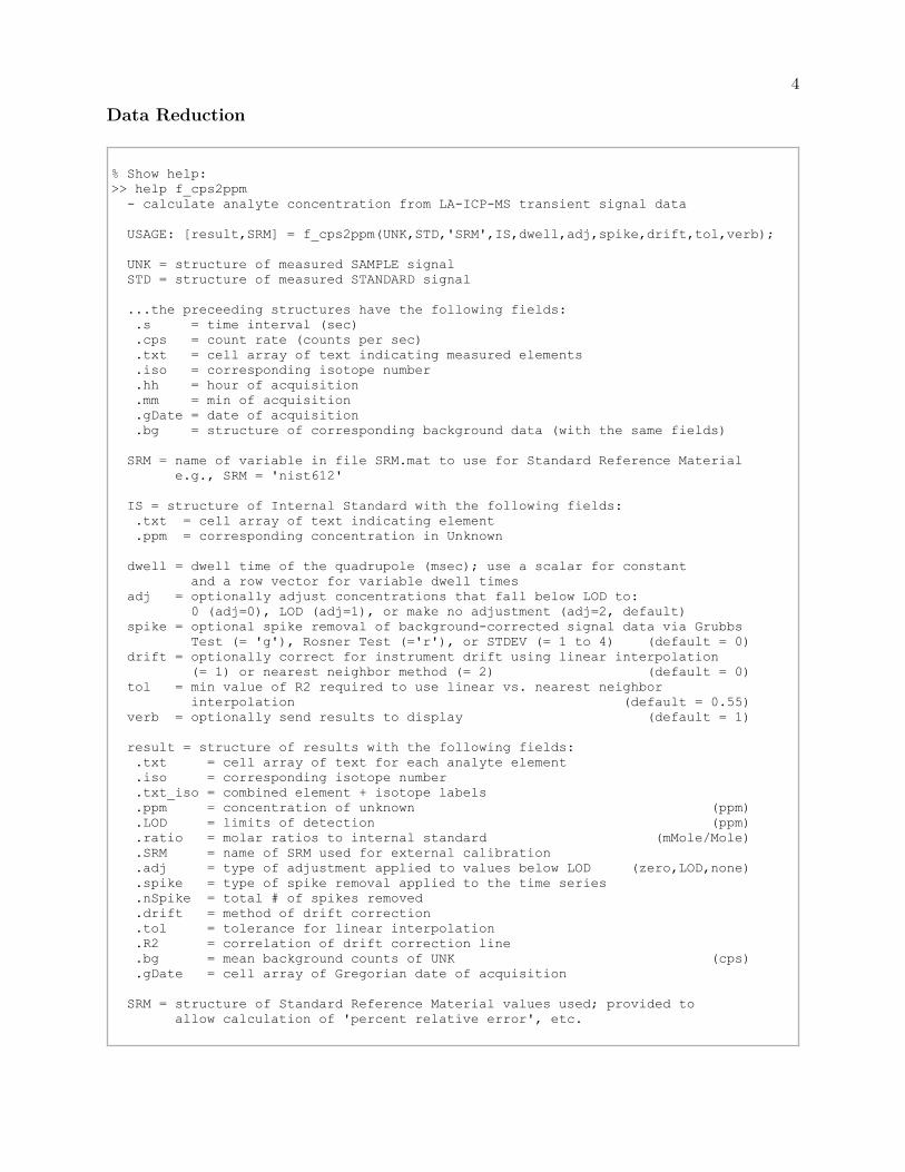
Data Reduction

% Show help:>> help f_cps2ppm - calculate analyte concentration from LA-ICP-MS transient signal data USAGE: [result,SRM] = f_cps2ppm(UNK,STD,'SRM',IS,dwell,adj,spike,drift,tol,verb); UNK = structure of measured SAMPLE signal STD = structure of measured STANDARD signal ...the preceeding structures have the following fields: .s = time interval (sec) .cps = count rate (counts per sec) .txt = cell array of text indicating measured elements .iso = corresponding isotope number .hh = hour of acquisition .mm = min of acquisition .gDate = date of acquisition .bg = structure of corresponding background data (with the same fields) SRM = name of variable in file SRM.mat to use for Standard Reference Material e.g., SRM = 'nist612' IS = structure of Internal Standard with the following fields: .txt = cell array of text indicating element .ppm = corresponding concentration in Unknown dwell = dwell time of the quadrupole (msec); use a scalar for constant and a row vector for variable dwell times adj = optionally adjust concentrations that fall below LOD to: 0 (adj=0), LOD (adj=1), or make no adjustment (adj=2, default) spike = optional spike removal of background-corrected signal data via Grubbs Test (= 'g'), Rosner Test (='r'), or STDEV (= 1 to 4) (default = 0) drift = optionally correct for instrument drift using linear interpolation (= 1) or nearest neighbor method (= 2) (default = 0) tol = min value of R2 required to use linear vs. nearest neighbor interpolation (default = 0.55) verb = optionally send results to display (default = 1) result = structure of results with the following fields: .txt = cell array of text for each analyte element .iso = corresponding isotope number .txt_iso = combined element + isotope labels .ppm = concentration of unknown (ppm) .LOD = limits of detection (ppm) .ratio = molar ratios to internal standard (mMole/Mole) .SRM = name of SRM used for external calibration .adj = type of adjustment applied to values below LOD (zero,LOD,none) .spike = type of spike removal applied to the time series .nSpike = total # of spikes removed .drift = method of drift correction .tol = tolerance for linear interpolation .R2 = correlation of drift correction line .bg = mean background counts of UNK (cps) .gDate = cell array of Gregorian date of acquisition SRM = structure of Standard Reference Material values used; provided to allow calculation of 'percent relative error', etc.

4

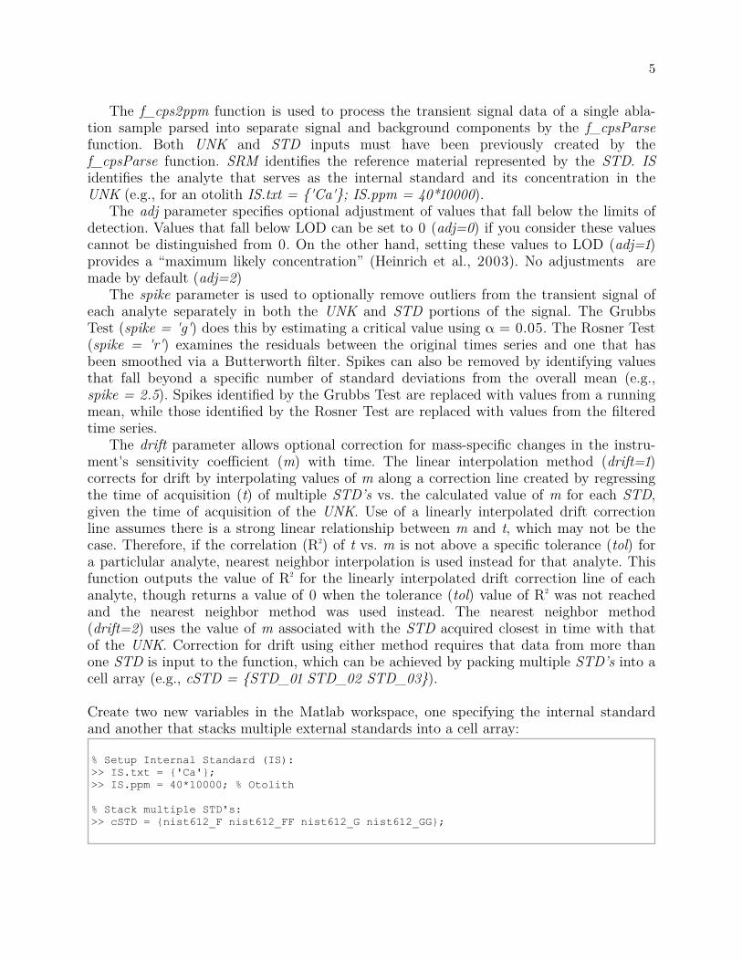
The f_cpsppm function is used to process the transient signal data of a single abla-tion sample parsed into separate signal and background components by the f_cpsParsefunction. Both UNK and STD inputs must have been previously created by thef_cpsParse function. SRM identifies the reference material represented by the STD. ISidentifies the analyte that serves as the internal standard and its concentration in theUNK (e.g., for an otolith IS.txt = {'Ca'}; IS.ppm = *).

The adj parameter specifies optional adjustment of values that fall below the limits ofdetection. Values that fall below LOD can be set to (adj=) if you consider these valuescannot be distinguished from . On the other hand, setting these values to LOD (adj=)provides a “maximum likely concentration” (Heinrich et al., ). No adjustments aremade by default (adj=)

The spike parameter is used to optionally remove outliers from the transient signal ofeach analyte separately in both the UNK and STD portions of the signal. The GrubbsTest (spike = 'g') does this by estimating a critical value using α = .. The Rosner Test(spike = 'r') examines the residuals between the original times series and one that hasbeen smoothed via a Butterworth filter. Spikes can also be removed by identifying valuesthat fall beyond a specific number of standard deviations from the overall mean (e.g.,spike = .). Spikes identified by the Grubbs Test are replaced with values from a runningmean, while those identified by the Rosner Test are replaced with values from the filteredtime series.

The drift parameter allows optional correction for mass-specific changes in the instru-ment's sensitivity coefficient (m) with time. The linear interpolation method (drift=)corrects for drift by interpolating values of m along a correction line created by regressingthe time of acquisition (t) of multiple STD’s vs. the calculated value of m for each STD,given the time of acquisition of the UNK. Use of a linearly interpolated drift correctionline assumes there is a strong linear relationship between m and t, which may not be thecase. Therefore, if the correlation (R) of t vs. m is not above a specific tolerance (tol) fora particlular analyte, nearest neighbor interpolation is used instead for that analyte. Thisfunction outputs the value of R for the linearly interpolated drift correction line of eachanalyte, though returns a value of when the tolerance (tol) value of R was not reachedand the nearest neighbor method was used instead. The nearest neighbor method(drift=) uses the value of m associated with the STD acquired closest in time with thatof the UNK. Correction for drift using either method requires that data from more thanone STD is input to the function, which can be achieved by packing multiple STD’s into acell array (e.g., cSTD = {STD_ STD_ STD_}).

Create two new variables in the Matlab workspace, one specifying the internal standardand another that stacks multiple external standards into a cell array:

% Setup Internal Standard (IS):>> IS.txt = {'Ca'};>> IS.ppm = 40*10000; % Otolith

% Stack multiple STD's:>> cSTD = {nist612_F nist612_FF nist612_G nist612_GG};

5

Perform standard data reduction of the transient signal data to generate mean analyte concentrations and molar ratios:

% Process data:% dwell = 10 ms : dwell time of the quadrupole% adj = 0 : adjust all values < LOD to 0% spike = 'r' : remove spikes using the Rosner Test% drift = 1 : correct for instrument drift using linear interp.% tol = 0.55 : R2 must be at least 0.55 to use linear interp.% verb = 1 : show results in display

>> f_cps2ppm(o20_A,cSTD,'nist612',IS,10,0,'r',1,0.55,1);

============================================================================== 'Analyte' 'ppm' 'LOD' 'mMole/Mole' '# spikes' 'Drift R2' 'Li7' [ 0.29579] [ 0.028704] [ 0.0042698] [ 0] [ 0.91308] 'Na23' [ 2648.6] [ 5.2702] [ 11.543] [ 0] [ 0.84286] 'Mg24' [ 18.849] [ 0.062083] [ 0.077704] [ 0] [ 0.97218] 'P31' [ 125.39] [ 4.5297] [ 0.4056] [ 0] [ 0] 'Ca43' [ 400000] [ 35.904] [ 1000] [ 1] [ 0] 'Sc45' [ 0.11601] [ 0.0908] [0.00025855] [ 4] [ 0] 'V51' [ 0.047926] [ 0.036853] [9.4264e-05] [ 0] [ 0] 'Cr53' [ 0] [ 0.27981] [0.00048098] [ 3] [ 0] 'Mn55' [ 0.099284] [ 0.073516] [0.00018107] [ 1] [ 0] 'Fe57' [ 219.95] [ 0.91298] [ 0.39462] [ 0] [ 0.84816] 'Co59' [ 0.22105] [ 0.014159] [0.00037582] [ 0] [ 0.96357] 'Ni60' [ 0.3063] [ 0.089473] [0.00052288] [ 4] [ 0] 'Cu63' [ 0.70591] [ 0.13112] [ 0.001113] [ 0] [ 0.75547] 'Zn64' [ 1.9096] [ 0.10614] [ 0.002926] [ 0] [ 0.59565] 'Cu65' [ 0.86246] [ 0.14063] [ 0.0013599] [ 0] [ 0.59897] 'Ge72' [ 0.15059] [ 0.12002] [0.00020772] [ 0] [ 0] 'Rb85' [ 0.082167] [ 0.017693] [9.6325e-05] [ 2] [ 0.80606] 'Sr88' [ 1880.6] [ 0.12195] [ 2.1505] [ 1] [ 0.86216] 'Y89' [ 0] [0.0045579] [3.7911e-06] [ 0] [ 0.99101] 'Cd114' [ 0.082234] [ 0.042774] [7.3297e-05] [ 1] [ 0] 'Sn118' [ 0.50128] [ 0.041494] [ 0.0004231] [ 0] [ 0] 'Ba137' [ 6.3626] [ 0.018038] [ 0.0046422] [ 0] [ 0.66995] 'Au197' [ 0] [0.0093391] [ 2.638e-06] [ 4] [ 0] 'Pb208' [ 0.34798] [ 0.042558] [0.00016827] [ 0] [ 0] 'Th232' [ 0] [0.0029745] [6.9857e-07] [ 1] [ 0.84554] 'U238' [0.0025237] [0.0022237] [1.0623e-06] [ 0] [ 0]

------------------------------------------------------------------------------SRM = nist612LOD adjustment = zeroSpike removal = Rosner TestDrift correction = linearNaN = analyte not present in SRM

Drift R2 is the correlation of the linearly interpolated drift correction line: 0 = indicates Nearest Neighbor interpolation was used instead - = indicates NO interpolation was performed------------------------------------------------------------------------------

6

Table 1. (A) The variables created in the Matlab workspace when clicking the signal button in theGUI created by the f_cpsParse command are structures, as shown here for the data collected bythe nist_FF spot scan. (B) The background button appends an additional structure to this vari-able under the field name .bg.

>> nist612_FF

nist612_FF =

s: [157x1 double] cps: [157x26 double] txt: {1x26 cell}

iso: [7 23 24 31 43 45 51 53 55 57 59 60 63 64 65 72 85 88 89 114 118 137 197208 232 238] hh: 16 mm: 51 gDate: {'09-Dec-2010'} idx: [716 872] bg: [1x1 struct]

>> nist612_FF.bg

ans =

s: [97x1 double] cps: [97x26 double] txt: {1x26 cell}

iso: [7 23 24 31 43 45 51 53 55 57 59 60 63 64 65 72 85 88 89 114 118 137 197208 232 238] hh: 16 mm: 51 gDate: {'09-Dec-2010'} idx: [587 683]

7

Figure . Annotated time chart printed from the Agilent Technologies ‘Data Analysis’ moduledepicting total ion count rates (cps) for the transient signal data exported to the file101209_B.csv. The first peak represents a false start when the scan sequence set in the laser abla-tion control software (i.e., Chromium) was paused in order to change the laser sampling parame-ters. All other scan sequences are bracketed by 60 s gas blanks and labelled as either spot scans ofexternal reference material (NIST or MACS) or otolith thin sections (samples 20–24, with n = 3replicates).

8

Figure . Graphical user interface (GUI) created by the f_cpsParse function to select and extractthe region of the raw ion count time series corresponding to the signal data collected while ablat-ing standard reference material nist612_FF. See Table 4A for the corresponding variable createdin the Matlab workspace.

9

Figure . Graphical user interface (GUI) created by the f_cpsParse function to select and extractthe region of the raw ion count time series corresponding to the background data collected priorto ablating standard reference material nist612_FF. See Table 4B for the corresponding variablecreated in the Matlab workspace.

10

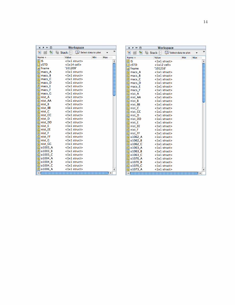
Figure . Matlab workspace showing the list of variables created by parsing the raw transient sig-nal data (raw_B) into separate signal/background components for the standard reference material(e.g., nist612_F, macs_G) and otolith samples (e.g., o20_A). Note that “_A” through “_C”represent replicate spot scans taken within the same otolith thin section. The NIST- SRMwas used as a calibration standard and the MACS was used to evaluate subsequent experi-ment-wise percent relative standard deviations (%RDS).

11

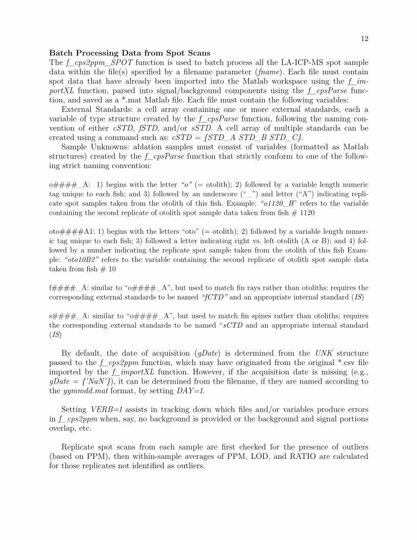
Batch Processing Data from Spot ScansThe f_cpsppm_SPOT function is used to batch process all the LA-ICP-MS spot sampledata within the file(s) specified by a filename parameter (fname). Each file must containspot data that have already been imported into the Matlab workspace using the f_im-portXL function, parsed into signal/background components using the f_cpsParse func-tion, and saved as a *.mat Matlab file. Each file must contain the following variables:

External Standards: a cell array containing one or more external standards, each avariable of type structure created by the f_cpsParse function, following the naming con-vention of either cSTD, fSTD, and/or sSTD. A cell array of multiple standards can becreated using a command such as: cSTD = {STD_A STD_B STD_C}.

Sample Unknowns: ablation samples must consist of variables (formatted as Matlabstructures) created by the f_cpsParse function that strictly conform to one of the follow-ing strict naming convention:

o####_A: 1) begins with the letter “o” (= otolith); 2) followed by a variable length numerictag unique to each fish; and 3) followed by an underscore (“_”) and letter (“A”) indicating repli-cate spot samples taken from the otolith of this fish. Example: “o1120_B” refers to the variablecontaining the second replicate of otolith spot sample data taken from fish # 1120

oto####A1: 1) begins with the letters “oto” (= otolith); 2) followed by a variable length numer-ic tag unique to each fish; 3) followed a letter indicating right vs. left otolith (A or B); and 4) fol-lowed by a number indicating the replicate spot sample taken from the otolith of this fish Exam-ple: “oto10B2” refers to the variable containing the second replicate of otolith spot sample datataken from fish # 10

f####_A: similar to “o####_A”, but used to match fin rays rather than otoliths; requires thecorresponding external standards to be named “fCTD” and an appropriate internal standard (IS)

s####_A: similar to “o####_A”, but used to match fin spines rather than otoliths; requiresthe corresponding external standards to be named “sCTD and an appropriate internal standard(IS)

By default, the date of acquisition (gDate) is determined from the UNK structurepassed to the f_cpsppm function, which may have originated from the original *.csv fileimported by the f_importXL function. However, if the acquisition date is missing (e.g.,gDate = {'NaN'}), it can be determined from the filename, if they are named according tothe yymmdd.mat format, by setting DAY=.

Setting VERB= assists in tracking down which files and/or variables produce errorsin f_cpsppm when, say, no background is provided or the background and signal portionsoverlap, etc.

Replicate spot scans from each sample are first checked for the presence of outliers(based on PPM), then within-sample averages of PPM, LOD, and RATIO are calculatedfor those replicates not identified as outliers.

12

>> help f_cps2ppm_SPOT - batch process parsed LA-ICP-MS spot data USAGE: [result,all] = f_cps2ppm_SPOT(fname,'SRM',IS,dwell,adj,spike,drift,tol,verb,match,day); fname = cell array of file(s) to process SRM = name of variable in file SRM.mat to use for Standard Reference Material e.g., SRM = 'nist612' IS = structure of Internal Standard with the following fields: .txt = cell array of text indicating element .ppm = corresponding concentration in Unknown dwell = dwell time of the quadrupole (msec); use a scalar for constant and a row vector for variable dwell times adj = optionally adjust concentrations that fall below LOD to: 0 (adj=0), LOD (adj=1), or make no adjustment (adj=2, default) spike = optional spike removal of background-corrected signal data via Grubbs Test (= 'g'), Rosner Test (='r'), or STDEV (= 1 to 4) (default = 0) drift = optionally correct for instrument drift using linear interpolation (= 1) or nearest neighbor method (= 2) (default = 0) tol = min value of R2 required to use linear vs. nearest neighbor interpolation (default = 0.55) verb = verbose output of progress (default = 1) match = regular expression pattern to match names of otolith spot scans 1: matches o1140_A (replicates A-C) (default = 1) 2: matches o1140_A (all replicates) 3: matches oto10A1 4: matches f1140_A (replicates A-C) 5: matches s1140_A (replicates A-C) day = determine date of acquisition from file name result = structure of results with the following fields: .oto = numeric tag identifying individual otoliths .txt = cell array of text for each analyte element .iso = corresponding isotope number .txt_iso = combined element + isotope labels .nRep = # within-otolith replicate spot samples used to calclate averages .ppm = concentration of unknown, averaged across replicates (ppm) .LOD = limits of detection, averaged across replicates (ppm) .ratio = molar ratios to internal standard, averaged across replicates (mMole/Mole) .SRM = name of SRM used for external calibration .adj = type of adjustment applied to values below LOD (zero,LOD,none) .spike = type of spike removal applied to the time series .drift = method of drift correction .tol = tolerance for linear interpolation .SRM = name of SRM used for external calibration .gDate = cell array of Gregorian date of acquisition all = structure of results (NOT averaged acrossed otoliths): .oto = numeric tag identifying individual otoliths .txt = cell array of text for each analyte element .iso = corresponding isotope number .txt_iso = combined element + isotope labels .ppm = concentration of unknown (ppm) .LOD = limits of detection (ppm) .ratio = molar ratios to internal standard (mMole/Mole) .bg = mean background counts of UNK (cps) .gDate = cell array of Gregorian date of acquisition

13

14

Citation for this document:Jones, D. . Processing LA-ICP-MS otolith microchemistry data using the FathomToolbox for Matlab. Technical Report ... Laboratory for Otolith Microchemistry.College of Marine Science, University of South Florida, St. Petersburg, FL. Available from:http://www.marine.usf.edu/user/djones.

Literature Cited

Halter, W., T. Pettke, C. A. Henrich, and B. Rothen-Rutishauser. . Major to traceelement analysis of melt inclusions by laser-ablation ICP-MS: methods ofquantification. Chemical Oceanography : –.

Henrich, C. A., T. Petke, W. E. Halter, M. Aigner-Torres, A. Audetat, D. Gunther, B.Hattendorf, D. Bleiner, M. Guillong, and I. Horn. . Quantitative multi-elementanalysis of minerals, fluid and melt inclusions by laser-ablation inductively-coupled-plasma mass-spectrometry. Geochimica et Cosmochimica Acta : –.

Jackson, S. E. . Chapter : Calibration strategies for elemental analysis by LA-ICP-MS. Pages – in Sylvester, P., editor. Laser Ablation–ICP–MS in the EarthSciences. Current practices and outstanding issues. Mineralogical Association ofCanada, Short Course Series Volume , Vancouver, B.C.

Jones, D. L. . The Fathom Toolbox for Matlab: multivariate ecological andoceanographic data analysis. College of Marine Science, University of South Florida,St. Petersburg, FL. Available from: http://www.marine.usf.edu/user/djones.

Koenig, A. E., and S. A. Wilson. . A marine carbonate reference material formicroanalysis. Proceedings of the First International Sclerochronology Conference, St.Petersburg, Florida, July –,

Longerich, H. P., S. E. Jackson, and D. Gunther. . Laser ablation-inductively coupledplasma-mass spectrometric transient signal data acquisition and analyte concentrationcalculation. Errata. J. Anal. At. Spectrom. : .

Longerich, H. P., S. E. Jackson, and D. Gunther. . Laser ablation-inductively coupledplasma-mass spectrometric transient signal data acquisition and analyte concentrationcalculation. J. Anal. At. Spectrom. : –.

Pearce, N. J. G., W. T. Perkins, J. A. Westgate, M. P. Gorton, S. E. Jackson, C. R. Neal,and S. P. Chenery. . A compilation of new and published major and trace elementdata for NIST SRM and NIST SRM glass reference materials. GeostandardsNewsletter : –.

15