United StatesDepartment ofAgriculture

Forest Service

ForestProductsLaboratory

ResearchPaperFPL–RP–558

Predictor Sort Sampling,Tight t 's, and theAnalysis of CovarianceTheory, Tables, and Examples

Steve P. VerrillDavid W. Green

Abstract ContentsIn recent years wood strength researchers have begun toreplace experimental unit allocation via random samplingwith allocation via sorts based on nondestructive measure-ments of strength predictors such as modulus of elasticityand specific gravity. Although this procedure has thepotential of greatly increasing experimental sensitivity, ascurrently implemented it can easily reduce sensitivity. Inthis paper we discuss the problem and we present solutions.Given the existence of nondestructive measurements ofstrength predictors, our methods can be used to reducesample sizes. We have written a public domain computerprogram that implements the methods.

Keywords: t distribution, paired t, pooled t, analysis ofcovariance, power, experimental design, sample size,asymptotics

October 1996

Verrill, Steve P.; Green, David W. 1996. Predictor sort sam-pling, tight t’s, and the analysis of covariance: Theory, tables,and examples. Res. Pap. FPL-RP-558. Madison, Wl: U.S. Depart-ment of Agriculture, Forest Service, Forest Products Labora-tory. 105 p.

A limited number of free copies of this publication are availableto the public from the Forest Products Laboratory, One GiffordPinchot Drive, Madison, WI S3705-2398. Laboratory publica-tions are sent to more than 1,000 libraries in the United Statesand elsewhere.

The Forest Products Laboratory is maintained in cooperationwith the University of Wisconsin.

The use of trade or firm names is for information only and doesnot imply endorsement by the U.S. Department of Agricultureof any product or service.

The United States Department of Agriculture (USDA) prohibitsdiscrimination in its programs on the basis of race, color, na-tional origin, sex, religion, age, disability, political beliefs, andmarital or familial status. Persons with disabilities who requirealternative means of communication of program information(braille, large print, audiotape, etc.) should contact the USDAOffice of Communications at (202) 720-2791. TO file a com-plaint, write the Secretary of Agriculture, U.S. Department ofAgriculture, Washington, DC 20250, or call (202) 720-7327(voice), or (202) 720-1127 (TTD). USDA is an equal employ-ment opportunity employer.

Page

Introduction . . . . . . . . . . . . . . . . . . . . . . . . . . . . . . . . . . . . . . . . . . . . . . . . . . . . 1

Mathematical Basis of Our Approach . . . . . . . . . . . . . . . . . . . . . . . . . . .3

Applying Our Methods . . . . . . . . . . . . . . . . . . . . . . . . . . . . . . . . . . . . . . . . . . . . . . . . . .3

Tables and a Computer Program . . . . . . . . . . . . . . . . . . . . . . . . . . . . .3

Example 1—A Simulated ExperimentUsing Our Methods . . . . . . . . . . . . . . . . . . . . . . . . . . . . . . . . . . . . . . . . . . ..4

Example 2—Estimating Power . . . . . . . . . . . . . . . . . . . . . . . . . . . . . . .7

Analysis of Variance/Covariance . . . . . . . . . . . . . . . . . . . . . . . . . . . . .8

Monte Carlo Estimates of Critical Values . . . . . . . . . . . . . . . . . . . . .9

Power Study . . . . . . . . . . . . . . . . . . . . . . . . . . . . . . . . . . . . . . . . . . . . . . . . . . . . . . . . . . . . . . . . . l O

Tight t’ s as “Partially Paired” t’ s . . . . . . . . . . . . . . . . . . . . . . . . . . . . . . . . . . . 12

References . . . . . . . . . . . . . . . . . . . . . . . . . . . . . . . . . . . . . . . . . . . . . . . . . . . . . . . . . . . . . . . . . . . 13

Appendix A—Proofs . . . . . . . . . . . . . . . . . . . . . . . . . . . . . . . . . . . . . . . . . . . . . . . 16

Appendix B—Tables . . . . . . . . . . . . . . . . . . . . . . . . . . . . . . . . . . . . . . . . . . . . . . . . . . . . . 18

Predictor Sort Sampling, Tight t’ s, and the Analysisof CovarianceSteve P. Verrill, Mathematical StatisticianDavid W. Green, Supervisory Research General Engineer

1 Introduction

In recent years wood strength researchers have begun to replace experimented unit allocation viarandom sampling with allocation via sorts based on nondestructive measurements of strengthpredictors such as modulus of elasticity and specific gravity. Warren and Madsen (1977) describethe procedure as follows:

One can take steps, however, to ensure that the inherent strength distributions of testand control samples are reasonably equivalent. Indeed, failure to do so can only throwdoubt on the results.

Specifically, then, all the boards in the experiment are ordered from weakest to strongestas nearly as can be judged from their moduli of elasticity, knot size, and slope of grain.To divide the material into J equivalent groups the first J boards, after ordering, aretaken and randomly allocated one to each group. This is repeated with the second,third, fourth, etc., sets of J boards. The strength distributions of the resulting groupsshould then be essentially the same.

Although this procedure is intuitively attractive, if the associated analysis does not take intoaccount the nonrandom nature of the sampling, the experiment can be less sensitive to treatmenteffects. We illustrate the problem with a simple example:

Suppose that a wood scientist wishes to test whether the mean strength of lumber treated withpreservative A differs from the mean strength of lumber treated with preservative B. Assume thatthe scientist has decided on samples of size k and has obtained 2k specimens from some source.Then, to make the initial samples of lumber as similar as possible, the scientist measures a predictorvariable (this could be a linear combination of modulus of elasticity (MOE), specific gravity, . . . ),orders the measurements

and labels the corresponding specimens

Next, for i = 1,..., k, the scientist randomly assigns one of {S2i_1, S2i} to treatment A and theother specimen to treatment B. This procedure should lead to nearly identical initial predictordistributions in the 2 samples. Believing that the predictor is well correlated with modulus ofrupture (MOR), the scientist hopes that the procedure will also lead to nearly identical initialMOR distributions. In accord with current practice, the scientist then proceeds with the experimentand analyzes the results as if the two initial samples were composed of independent, identicallydistributed representatives of an initial strength distribution. Given this (incorrect) distributional

1

assumption, an appropriate test for a postpreservative difference in mean strength would be apooled t test.

Contrary to the scientist’s intuition, this approach can actually decrease one’s ability to detecta difference between the two preservatives. Why the decrease? Given the standard assumptions ofnormality and independence, the test statistic

has a nulll t distribution with 2k – 2 degrees of freedom. However, when the sampling is viaa predictor sort, r is no longer distributed as a t. Instead the distribution depends upon thecorrelation ρ ρ between the predictor variable and the response variable. As this correlation increasesto 1, the null distribution of ~ will “tighten” around 0. In Figure 1, we present a histogram2 of Tvalues for the predictor sort case in which k = 24 and ρ ρ = .70. Superimposed on the histogram isthe probability density function of a standard t distribution with 46 degrees of freedom. Clearly,the t distribution overestimates the “width” of the true distribution.

Now an analyst who is ignoring the nonrandom nature of the sampling will use 2.013 (froma standard t table) as the critical value for a test of the hypothesis that there is no differencein the strength properties associated with treatments A and B. Let ∆ ∆ denote the true, unknowndifference between the mean strengths of the two types of wood, and let σ σ denote the true standarddeviation of the strength. For ∆ ∆ / σ σ sufficiently small, the narrowing of the ~ distribution will reducethe chance of detecting an effect. On the other hand, for ∆ ∆ / σ σ sufficiently large, it will increasethe chance.3 This result is illustrated in Figure 2. There the dashed line4 represents the powers

associated with a predictor sort design followed by a standard (but incorrect) analysis using a 2.013critical value. The solid line represents the power associated with a standard random samplingdesign followed by a standard analysis.

If the correct critical values are used (we obtain these below), then the predictor sort procedureyields a power curve that is uniformly better than the power curve obtained in the random samplingcase. For the k = 24, ρ ρ = .7 case, this curve is plotted as the dotted line in Figure 2. As we willsee below, this increased power can yield substantial sample size savings.

In the next section we obtain the asymptotic (large sample) distributions of the “pooled tightt“ and the “paired tight t.”

In Section 3 we work through several examples of predictor sort/tight t design and analysisprocedures. We have written a public domain computer program that implements these procedures.

1The “null” distribution is the distribution of the test statistic under the “null hypothesis” — no differencebetween treatments.

2The histogram was obtained via computer simulation and is based on 4,000 trials.3The relative narrowness of the r distribution means that right tail values tend to be pulled down and left tail

values tend to be pulled up. Thus, roughly speaking, if A/(o@) is less than 2.013, T will be less likely to lieabove the critical value than a standard t statistic, while if A/(u@) is greater than 2.013, r will be more likelyto lie above the critical value than a standard t statistic.

4For the cases ∆ ∆ / σ σ = 0.0, 0.075, 0.150, 0.225, . . . . 1.5, 4000 samples of total size 48 were generated and then dividedinto subsamples of size 24 via a predictor sort with ρ ρ = .7. The r statistics were then calculated, and the frequencywith which these statistics fell beyond the -2.013,2.013 bounds was noted. The resulting 21 estimated power valueswere connected to yield the dashed line.

5The power of a statistical test is the probability (ranging from 0 to 1) that the test will reject the null hypothesisof no difference, that it will “detect a difference.” As the actual difference increases or the sample size increases, thepower will increase. One can also increase power by using an improved statistical method. A predictor sort followedby a tight t analysis constitutes one such method.

2

The program is described by Verrill, Green, and Herian [in press] and may be obtained from theauthors. See Section 3 for details.

Readers who are primarily interested in the application of our methods should restrict theirattention to Section 3.

The work that forms the basis for the computer program is discussed in Sections 4–6 andAppendix A. In Section 4 we present estimates of the small sample critical values of the tight t’ sand identify the sample sizes needed to permit use of the asymptotic (large sample) critical values.In Section 5 we present a power study that should be useful in selecting sample sizes, and we showthat we need not greatly concern ourselves about entering the critical value tables via estimates ofρ ρ . We include in this power study an analysis of covariance approach and identify those cases inwhich it is inferior to one of the tight t approaches. Finally, in Section 6 we warn against intuitivelyattractive, but incorrect, power calculations.

2 Mathematical Basis of Our Approach

We record here a theorem that justifies our approach to designing “tight t“ experiments andanalyzing “tight t“ data. Its practical import is explored in the sections that follow. If you simplywant to know how to use the result, please skip ahead to the next section.

Theorem. Assume that the predictor variable and the variable of interest have a joint bivariatenormal distribution with correlation ρ ρ . Let the allocation of samples be as described in Section1. (For a multiple factor case, enough adjacent experimental units would be chosen at a time toprovide one additional observation for each cell. ) Then, for – 1 < ρ ρ < 1, the asymptotic distributionof the statistic that treats the groups of “equivalent” experimental units as a block (the “pairedapproach”) is X2

J-1. The asymptotic distribution of the statistic that ignores the block structuregenerated by these groups (the “pooled approach”) is (1 – ρ ρ 2)X2

J-1.

Proof. The proof appears in the Appendix.

Note: Let T denote the usual pooled t statistic. Then T/~~2 is the “pooled tight t“statistic. The “paired tight t“ statistic has the same form as the usual paired statistic. By the

3 Applying Our Methods

reasoning used to prove the more general theorem just stated, one can show that given predictorsort sampling, for – 1 < ρ ρ < 1, the pooled tight t and the paired tight t are asymptotically N(0,l).

3.1 Tables and a Computer Program

To apply our methods, one can take a “manual” approach and use Tables 1 - 56 provided inAppendix B. In sections 3.2 and 3.3 we work through two examples.

Alternatively, one can use a computer program that we have written. This program performssample size calculations, specimen allocations, and data analyses. It can be run over the WorldWide Web — see http://www1.fpl.fs.fed.us/ttweb.html6.

6The program is in the public domain and can be obtained from the authors. Source code is available as are exe-cutable versions for Sun Solaris 1.x, Sun Solaris 2.x, and DOS. A user can obtain the program and annotated input tothe program (Verrill, Green, and Herian [in press]) via the World Wide Web (http://www1.fpl.fs.fed.us/papers.html),or via the U.S. Postal Service (USDA Forest Products Lab, 1 Gifford Pinchot Drive, Madison, WI 53705 — pleasesend us a floppy and specify the operating system). If you have questions about the program or encounter difficultiesin running it, please contact us at steve@ws13.fpl.fs.fed.us.

3

3.2 Example 1 — A Simulated Experiment Using Our Methods

In this section we work through an example of a predictor sort/tight t experiment. 7

Suppose that a scientist wants to determine whether there is a difference in the effects ofpreservatives A and B on MOR. In an effort “to reduce random variation between specimens inthe two groups,” the MOE values of all specimens will be determined prior to treatment. Thesevalues will be ranked from high to low. Pairs of specimens with adjacent MOEs will be randomlyseparated into the two treatment groups. Before any of this can be done, however, the scientistmust determine how many specimens will be needed.

3.2.1 Design — Sample Size Calculations

The scientist wants to choose a total sample size n = 2k sufficient to detect a 10% difference inmean strength at a .05 significance level with a probability of at least .90. The scientist believesthat the coefficient of variation of MO R is approximately 20%, and the correlation ρ ρ between MORand MOE is .70. (Here we use MOE as the predictor, but other variables or linear combinationsof variables could be used.)

There are three approaches that one could take to calculating an appropriate sample size— table, noncentral t, normal approximation. For lower ρ ρ , or for high ρ ρ and large sample sizecombinations, the three approaches will yield essentially the same results. We give examples of allthree approaches because they differ in ease of implementation, and because the latter two methodsare suspect for high ρ ρ , small sample size combinations (see Section 5).

Power Tables

Table 49 contains power results for a correlation of .70. (A detailed description of the tables isprovided in the Index to the Tables that appears at the beginning of Appendix B.) The differenceA that we want to be able to detect is approximately .10 × µ where µ is the mean MOR ofthe specimens. Also, since the coefficient of variation, σ σ / µ × 100, is approximately 20%, σ σ N(is approximately) 0.20 × µ. Thus ∆ ∆ / σ σ x 0.5. Looking in the “Tight t /Unknown ρ ρ /Pooled/ ρρestimated” column in Table 49, we see that the power for a total sample size of 72 (72 = n = 2k)and ∆ ∆ / σ σ = .5 is .84. For a total sample size of 96 and ∆ ∆ / σ σ = .5, the power is .92. Interpolatingbetween these two values we see that we would need about

total observations to assure ourselves of a .90 probability of detecting a 10% difference in meanstrength. (For ρ ρ = .70, ∆ ∆ / σ σ = .5, n = 90, a standard random sampling approach would only yielda power of .55 + (.68 – .55)(90 – 72)/(96 – 72) x .65 — see Table 49.)

Noncentral t

As noted in Section 5, the noncentral t approach works best for ρ ρ < .80. As ρ ρ approaches 1, thisapproach yields an overestimate of power and thus an underestimate of needed sample size.

7One can also take an analysis of covariance approach to this problem. As we will see in the power study, providedthat the relationship between the predictor and MOR is correctly modelled, an analysis of covariance approach willalso yield good power properties.

4

For this example, the noncentrality parameter is

The power is then

where t γ γ is a noncentral t statistic with noncentrality parameter γ, γ, and t2k-2 (.025) is the one-sided.025 critical value for a central t with 2k – 2 degrees of freedom. Our computer program performsthis calculation (as well as the other calculations associated with the design and analysis of apredictor sort experiment) and yields n = 88.

Normal Approximation

As noted in Section 5, the normal approximation approach is even more susceptible to overesti-mating power — underestimating sample size — than the noncentral t approach. However, thisdoes not appear to be a problem for lower ρ ρ and higher n (e.g., see Table 49), and to implementthe method we need only a table of the normal cumulative distribution function.

For the current example, we have

where s pooled is the pooled standard deviation, and N(0,l) denotes a standard normal distribution.Thus, the approximate power is

We can neglect the first term in this sum, set the second term equal tosolve for k. For our example this yields

the desired power, and

5

We see that, for this example, the three methods give similar results. For ρ ρ < .8 and n > 24 (say)this is to be expected. (See the power tables.)

3.2.2 Design — Specimen Allocation

For the example, MOR, MOE pairs were generated from a bivariate normal distribution with meanvector

and covariance matrix

where σ σ MOE = .2 × µ MOE and σ σ MOR = .2 × µ MOR. In Table 56, we list the 90 MOE,MOR pairsas drawn, the 90 pairs ordered by MOE, and the division of the data into two sets of 45 pairs.(In addition to performing sample size calculations, the computer program described above alsosorts predictor values and then randomly allocates adjacent experimental units to the two testconditions. ) In Table 56, we also list “treated” MOR values. For treatment B, these are the sameas the untreated values. For treatment A, they have been reduced by 500 from the untreatedvalues.

3.2.3 Analysis

Given the values listed in Table 56, the estimate of ρ ρ is

The pooled estimate of the MOR standard deviation is

The pooled tight t statistic is

This value should be compared to a critical value appropriate to a pooled tight t statistic withρ ρ = .72, n = 2k = 90, and (two-sided) size equal to .05. This critical value can be obtained inseveral ways. One approach is to note that n = 90 which, according to Table 17, is large enough thatwe may use a standard normal distribution table to find the critical value. Thus we are justified incomparing 2.99 with z (.05/2) = 1.96 and concluding that there is a significant difference betweenthe two treatments.

6

Alternatively, when we cannot use large sample results, we can use Tables 1-10 (and Table 11)to calculate the critical values for pooled (Tables 1–5) and paired (Tables 6-10) tight t statistics.For example, if the correlation between predictor and response (e.g., MOE and MOR) were .70,and one wanted to use the pooled tight t with total sample size equal to 90, and to do a test at a5% significance level, then one would use the values in the .70 row of Table 3, and the equation

to obtain the critical value

For n = 90 and ρ ρ = .75, we have

An interpolation (which is even simpler than usual in this case) yields 1.99 as an appropriateestimate of the critical value. Since 2.99 > 1.99, we can conclude that there is a significantdifference between the two treatments. (The computer program described above will also calculatethe t value, find the appropriate critical value, and report the appropriate conclusion. )

3.3 Example 2 — Estimating Power

Winandy and others (1992) proposed to investigate the effects of preservative treatments on se-lected hardwoods and two types of laminated veneer lumber. Because they had limited suppliesof material, the authors were forced to restrict replication numbers to 16, 18, or 20, dependingupon the the particular treatment/drying condition/material combination in question. The authorswanted to be able to detect 10% differences in MOR. They believed that a reasonable estimateof the coefficient of variation for their material was .16, and that a reasonable estimate of thecorrelation between MOE and MOR was .7. What kind of power could they expect?

3.3.1 Standard Random Sampling Pooled T

We have ∆ ∆ / σ σ = .10/.16 = .625. Interpolating (quadratically in ∆ ∆ / σ σ and then quadratically in n)in the “Standard random sampling pooled t“ column of Table 49, one can see that approximatevalues for the powers are the following:

Using our Fortran program (with ρ ρ set to 0), we obtain the following:

7

Thus, if Winandy and others had performed standard random sampling and standard pooledt analyses, they would have had less than a 50% chance of detecting 10% mean differences. (Thisassumes that the authors wanted to compare individual “cells” in the desing. In the absence ofinteractions it would generally be possible to combine data from separate cells to achieve increasedpower.) There is a greater than 50% chance that they would have had to report no statisticallysignificant differences (at a .05 significance level) even if there really were 10% differences in pop-ulation means.

3.3.2 Tight t Approach

We have ∆ ∆ / σ σ = .10/.16 = .625. Interpolating (quadratically in ∆ ∆ / σ σ and then quadratically inn) in the “Tight t /Unknown ρ ρ /Pooled/ ρ ρ from experience” column of Table 49, one can see thatapproximate values for the powers are the following:

Using the noncentral t approach in our Fortran program (with ρ ρ set to .7), we obtain thefollowing:

Thus, by combining predictor sort sampling with a tight t analysis, Winandy and others in-creased their chances of detecting 10% mean differences by a factor of 1.5.

3.4 Analysis of Variance/Covariance

In actual practice, researchers seldom compare only two treatments. In general, there are multiple“factors” (e.g., chemical concentration, adhesive type, drying procedure) that are tested at multiple“levels.” For example, if there were three factors, each of which were tested at two levels, then thedesign would be a 2 × 2 × 2. If there were r replicates in each of the 2 × 2 × 2 = 8 cells, 8 × rspecimens would be needed to perform the experiment.

Taking a predictor sort approach, one would order the 8 × r specimens on the basis of anondestructive predictor such as MOE, take the top 8 specimens and randomly assign them to the8 cells, take the next 8 specimens and randomly assign them to the 8 cells, and so on.

To analyze these data one would take one of three approaches:

1. Use a standard unblocked analysis of variance (ANOVA) program, but replace the F valuesreported in the program by F /(1 – ρ ρ 2) values, where ρ ρ is the correlation between the predictorand the property being investigated.

2. Use a standard blocked analysis of variance in which the blocks were the groups of 8 specimenswith similar predictor properties. (Note that one would have to keep track of which specimenswere in which blocks.)

8

3. Perform a standard analysis of covariance (ANOCOV) using the predictor as the covariate.(Note that one would have to keep track of the value of the predictor for each specimen.)

The first two analysis approaches are only approximate for smaller sample sizes.Our computer program performs power calculations and specimen allocations for this more gen-

eral case. (Currently it can handle at most 5 factors, a total of 25 levels, and 5,000 specimens.) Theprogram does not perform analyses for multiple factor experiments, but ANOVA and ANOCOVprograms that do perform such analyses are readily available (e.g., the SAS GLM procedure).

4 Monte Carlo Estimates of Critical Values

We ran 10,000 trials for each combination of n = 2k = 4,6,8(4)40(8)120, 160, 200, 300 and ρρ= .40( .05).95, .99, 1.0. (The notation “8(4)40” stands for “from 8 to 40 in steps of 4.”) (Here,k is the number of observations per treatment, and ρ ρ is the correlation between the predictor xand the response y). To do so we used the uniform (UNI) and normal (RNOR) random numbergenerators developed by James Blue, David Kahaner, and George Marsaglia8 The absolute valuesof the scaled pooled statistic (the usual pooled statistic divided by ~~7) and the usual pairedstatistic were ordered, and order statistics 8001, 9001, 9501, 9801, and 9901 were used as estimatesof the two-sided .20, .10, .05, .02, .01 critical values. Using the techniques described in Verrill andJohnson (1988), one can see that this approach yields the following .999 probability intervals onthe true sizes: [.187,.213], [.090,.110], [.043,.057], [.015,.025], and [.0066,.0134] (e.g., prob( ξ ξ .090 <.10 cv estimate < ξ ξ .110) = .999).

For each ρ ρ /size (.20, .10, .05, .02, or .01) combination, the critical values for n = 8(4)40(8)120,160, 200, 300 were smoothed via the equation cvwas fixed at the appropriate asymptotic criticzd value.

For ρ ρ = 1 (not covered by the Theorem), there are heuristic reasons for believing that times the usual pooled statistic converges in distribution to something approximating a linearcombination of independent double exponentials. Thus, in this case, we calculated the smootherof the Monte Carlo critical values of the usual paired statistic, but we calculated the smoother ofthe Monte Carlo critical values of times usual pooled statistic.To perform the pooled ρ ρ = 1 calculations, we fixed ~ at the average of the estimated criticalvalues for n = 104, 112, 120, 160, 200, 300. (Plots indicated that the critical values seemed tohave leveled off at an “asymptotic value” by n = 104. ) In the paired r = 1 case, a. was a freeparameter that was estimated in the smoothing process. The coefficients for the pooled statisticsare presented in Tables 1–5. Those for the paired statistics are presented in Tables 6–10. Sincethe smoothing equations do not perform well for n < 8, the critical values for n = 4 and 6 andsize .05 are presented in Table 11. (Again the critical values reported in Table 11 for ρ ρ = 1 are thecritical values of the usual paired statistic, but the critical values of times the usual pooledstatistic. )

The quality of the smoothed critical values was tested by performing an additional 10,000 trialsfor each n, ρ ρ combination. Counts of the cases in which the smoothed critical values were exceededare summarized in Tables 12 and 13. To understand these tables one needs to note that if thesmoothed critical values were exact, then one would expect that

● 95% of the .20 two-sided size counts (for different n, ρ) ρ) will lie between 1922 and 2079,

8See the National Institute of Standards and Technology’s World Wide Web Guide to Available MathematicalSoftware at http://gams.nist.gov

9

● 95% of the .10 two-sided size counts will lie between 942 and 1060,

● 95% of the .05 two-sided size counts will lie between 458 and 544,

● 95% of the .02 two-sided size counts will lie between 173 and 228, and

● 95% of the .01 two-sided size counts will lie between 81 and 120.

(These limits are obtained using the arcsin square root transformation on the exceedance fraction.)For a given ρ ρ there are 22 × 5 = 110 n ,size combinations (we exclude n = 4,6 as they were notincluded in the smoothing calculation). The values in the column headed by “-” in Tables 12–16indicate the number of times among the 110 that the counts fell below the 9570 limits. The valuesin the column headed by “+” indicate the number of times that the counts fell above the limits.The values in the column headed by “0” indicate the number of times that the counts fell withinthe limits. The values in the column headed by .20 are the minimum and maximum over n =8(4)40(8)120, 160, 200, 300 of the exceedance counts for the two-sided .20 critical values. Similarremarks hold for the columns headed by .10, .05, .02, and .01. It is clear from Tables 12 and 13that if one uses the smoothed critical values, the two-sided size will not be off by more than .01for sizes .20 and .10, and .005 for size .05. In fact these figures are fairly conservative (as can beseen by the frequency with which the counts fall within the 95% limits).

In Table 14 we present the corresponding results for the case in which “incorrect t values” areused — we calculate a pooled t statistic that is not divided by ~~ and compare it to standardt values, In this case it is clear that actual sizes fall far below nominal sizes. The resulting powerloss is discussed in Section 5.

In Tables 15 and 16 we present the results for the cases in which “correct t values” are used (thepooled t statistic is divided by <~z before it is compared to standard t values). In the pooledcase, the tabled t values yield good approximations to the critical values of the scaled statistic forρ ρ < .80. In the paired case, the t approximation is satisfactory for ρ ρ as large as .90. For low n,however, as ρ ρ increases beyond .90, the actual size falls below the nominal size and a small amountof power (less than or equal to .15) is lost.

To get an idea of the sample sizes needed for the asymptotic critical values to be satisfactory,for each ρ ρ /size combination we fit a curve of the form a.+ al/n1i2 + a2/n + a3/n3/2 to the countsof the times that the asymptotic critcal values were exceeded in the 10,000 trials. (The value UQwas fixed at 2000, 1000, 500, 200, or 100, depending on the size in question.) We then found then’ s at which these curves descended below 2200, 1100, 550, 250, or 125. These values are reportedin Table 17 for the pooled T and in Table 18 for the paired T. Note that as the size decreases or ρρincreases (for the pooled case), the n needed to achieve good performance of the asymptotic valuesalso increases. On the other hand, for all but the highest ρ ρ , good performance is achieved for fairlysmall n (less than 100 in the pooled case).

5 Power Study

We performed a power study that covered the cases in which ρ ρ = .4(.1) .8, .85(.05 ).95, .99, n = 2k= 12(12)48, 72, 96, ∆ ∆ / σ σ y = 0.0(.25)1.5, and ρ ρ = .4(.1).8, .85(.05 ).95, .99, n = 2k = 4(2)14, ∆ ∆ / σ σ y

= 0.0(.5)3.0. Here ∆ ∆ is the mean difference between treatment 1 and treatment 2, and a; isthe variability of the y’s. The results of the study are presented in Tables 19 – 54, and can besummarized as follows:

● Using a predictor sort followed by a standard analysis yields poor power properties.

10

● The gain in efficiency of the tight t (pooled or paired) predictor sort approach over a standardrandom sampling approach ranges from 33% to 800% as r increases from .5 to .99.

● For the ρ ρ = .7 case (common in wood strength research) sample sizes may be (approximately)halved by using a tight t approach.

● Because of the difference in degrees of freedom, the pooled approach yields greater powerthan the paired approach. For small n, the gain can be substantial (e.g., for a = .01, n = 8,ρ ρ = .7, and ∆ ∆ / σ σ y = 2.5, the paired tight t yields power .42 while the pooled tight t yieldspower .81).

● For ρ ρ < .85, the pooled tight t performs as well as an analysis of covariance. (The analysisof covariance is based on the model y~j = aj + bzij + ~ij and tests whether al = az. Here ydenotes, for example, MOR, and x denotes, for example, MOE.) For small n (say, n < 14)the pooled tight t actually performs better than an analysis of covariance (e.g., for a = .01,n = 6, ρ ρ = .4, and ∆ ∆ / σ σ y = 3.0, a predictor sort followed by an analysis of covariance yieldsa power of .29, while the pooled tight t yields power .45. ).

● In the pooled case, for n > 12, ρ ρ < .95, entering the critical value tables via estimatedρ ρ 's causes no problems. (In our simulations, for each trial, r was calculated as the averageof the correlation between the predictor and the response for the treatment 1 sample, andthe correlation between the predictor and the response for the treatment 2 sample. For jiless than .40, standard t tables were used to obtain critical values. For j between .40 and.90, the interpolation was linear between the two nearest bracketing r ’s. For ~ greater than.90, the critical value was a quadratic interpolation/extrapolation of the critical values forρ ρ = ,90,.9.5, and .99.)

For n < 12, ρ ρ < .95, entering the tables via p can yield inflated sizes, but if ρ ρ is known fromexperience to within .05–.10, nominal and actual sizes match well. (In our simulations, foreach trial, “ ρ ρ from experience” was drawn from a N( ρ ρ , .052) distribution for ρ ρ < .90, from aN( ρ ρ , .0252) distribution for .90 < ρ ρ < .95, and from a N( ρ ρ , .0052) distribution for ρ ρ = .99.)

For ρ ρ = .99, entering the tables via ~ yields inflated sizes, but the inflation decreases toacceptable levels as n increases. For ρ ρ = .99, entering the tables via a ρ ρ “known fromexperience” is unacceptable.

● Entering the critical value tables via estimated ρ ρ ’s causes no problems in the paired case.

● For the pooled tight t, power results can be approximated well by taking a noncentral tapproach with noncentrality parameter equal to

and 2k – 2 degrees of freedom. Alternatively, power can be estimated by assuming thatThe noncentral t approach yields perfectly

adequate approximations to the true power for ρ ρ < .80, For higher ρ ρ it tends to overestimatepower, but the overestimation decreases as n increases. The normal approach yields a moresignificant overestimate of power, and its use should probably be restricted to lower ρ ρ andhigher n.

● Similarly, for the paired tight t, power results can be approximated by taking a noncentral tapproach with the same noncentrality parameter as in the pooled tight t case, but with k – 1

11

degrees of freedom. Also, power can be estimated by the same normal approximation used inthe pooled tight t case. Again, the noncentral t approach yields good power approximationsfor ρ ρ < .80 and for higher ρ ρ , n combinations. The power overestimation associated with thenormal approach is, of course, even more pronounced in the paired case.

● The noncentrality parameter associated with a two treatment analysis of covariance is

Thus it pays to minimize X.2 – X.l. For this reason, an analysis of covariance associatedwith predictor sort sampling performs slightly better (a .01–.10 increase in power) than ananalysis of covariance associated with a standard random allocation.

● If the relationship between the predictor and the response is misspecified, then, even for veryhigh ρ ρ , the tight t’ s can yield better power than an analysis of covariance. For moderaten, the misspecification can be difficult to detect. For example, for ρ ρ = .95, n = 24, and∆ ∆ / σ σ y = 0.0(.1).8, we list the powers associated with tight t analyses ( ρ ρ estimated from thedata) and an analysis of covaiance in Table 55. The table is based on 10,000 computersimulation trials per ∆ ∆ / σ σ value. The data sets for this analysis were generated by drawing24 x values from a N(20,72) distribution, and obtaining y values from y = x3 + c where thee’s were N(0, σ σ 2) with σ σ chosen so that the sample correlation between the x ’s and y’s wasapproximately .95. An example of such a data set is presented in Figure 3.

Caveats

These conclusions do not necessarily hold for very small n (e.g., n < 12). If a user wishes towork with samples of this size, the user should look to Tables 19–27 and 37–45 for specific guidance.Also, note that critical values obtained from Tables 1-10 do not perform well for n = 4; instead,see Table 11. (Tables 1 – 10 are based on smoothing curves fit to Monte Carlo critical valuesobtained for n > 8. See Section 3. These curves do not extrapolate well down to n = 4.)

6 Tight t ’s as “Partially Paired” t ’s

It is edifying to see how the noncentrality parameter described in Section 5,

differs from those in the “pure” pooled and paired cases. (Bear in mind, however, that asp increasesto 1, the noncentral t approach to estimating power loses validity.) Consider the following errormodel:

where Y is the property of interest, X is the predictor, are independentrandom variables with means equal to 0 and variances equal to (Thus,

Here σ σ represents the “natural variation” shared by Y and X.

12

represent the natural variation unique to Y and X. are the measurement errors. In thiscase the noncentrality parameter appropriate to a pure pooled t analysis would be

The noncentrality parameter that it is possible that a statistician would recommend and that itit is likely that a scientist would use (incorrectly) to calculate the sample sizes needed for a purepaired t analysis would be

Since the noncentrality parameter that one would use (correctly) tocalculate the sample sizes needed for a predictor sort experiment would be

We see from this that the predictor sort approach succeeds in partially blocking out natural vari-ation If is large in comparison to and is high), then the tight t noncentralityparameter is much larger than the pure pooled noncentrality parameter — the tight t yields a largeincrease in power. However the the predictor sort approach does not succeed in blocking out allnatural variation (the remain), and if is not small in comparison to “standard” paired tpower calculations can seriously underestimate the sample sizes needed.

References

13

Figure 1: Histogram of r for a correlation equal to .70 and total sample size of 48 (24 pertreatment) overlayed with the density function of a standard t distribution with 46 degrees offreedom.

Figure 2: Power comparison. Here the correlation between the property and the predictor value is.70. The total sample size is 48 (24 per treatment). A is the difference between the mean responsesfor the two treatments. σ σ is the standard deviation of the response. The solid line is the powercurve for standard random sampling followed by a standard pooled t analysis. The dashed lineis the power curve for a predictor sort allocation followed (incorrectly) by a standard pooled tanalysis, The dotted line is the power curve for a predictor sort allocation followed (correctly) bya pooled tight t analysis.

14

Figure 3: 24 (x, y) pairs where x is drawn from a N(20,72) distribution,from a N(0,a2) distribution, and σ σ is chosen so that the sample correlation between x and y isapproximately .95.

is drawn.

15

Appendix A — Proofs

Let H denote the inverse of the N(0,l) distribution function.

Lemma. Let U 1 n denote the first order statistic from a sample of n Uniform(0,l)’s. Thenconverges in probability to 0.

Proof. Since converges in distribution to an extreme value dis-tribution, and see, for example, Section 9.3 of David (1981)), the lemmafollows.

Proof of the Main Result

For ease of exposition, we will present the proof for the one-way case. The extension to a proof ofthe n-way case is straightforward.

Since the ANOVA F statistics are invariant under changes in location and scale it is clear that wecan obtain statistics that have the relevant distributions by ordering the X’s, bringing along theY’ s, and randomly dividing among the J treatments. (Here, Yl,n is the l thorder statistic among the Y’ s. )

Let Wij denote the i th Y that is assigned to treatment j. Thenwhere are i.i.d. N(0,l) and are independent of the X’ s.(Here, Xl,n is the l th order statistic among the X ’s.)

6.1 The Numerator of the F S t a t i s t i c s

The numerator of both the blocked and unblocked F statistics equals whereI = n/J. This equals

Now

which converges in probability to zero by the Lemma. Also, it is clear thatThese results, together with the Cauchy-Schwarz inequality, imply that

(1)

16

6.2 The Unblocked F D e n o m i n a t o r

We have

It is clear that the first term in the last sum converges to 1 in probability as I = n/J goes toinfinity. By (1), the second term in the last sum converges in probability to zero, so the unblockeddenominator coverges in probability to 1.

6.3 The Blocked F Denominator

We have

(2)

By (1), the last term in equation (2) converges in probability to zero as I = n/J goes to infinity.The first term equals

Clearly,

the Lemma, together with the Cauchy–Schwarz inequality, implies that the first term in equation(2) converges in probability to 1- ρρ 2

. Making one last use of the Cauchy–Schwarz inequality (toshow that the second term in equation (2) converges in probability to zero), we see that the blockeddenominator converges in probability to 1 – ρ ρ 2.

17

Appendix B — Tables

Index to the Tables

● Smoothing curve coefficients

– Pooled t, Tables 1–5

- Paired t, Tables 6-10

These tables can be used to calculate the critical values for pooled or paired tight t statistics.For example, if the correlation between predictor and response (e.g., MOE and MOR) were.7, and one wanted to use the pooled tight t with total ( n = 2 k ) sample size equal to 30, andto do a test at a 5% significance level (a .05 “size”), then one would use the values in the .70row of Table 3, and the equation

critical value =

to obtain the critical value

2.067 = 1.960 – .02812 /301/2 + 2.638/30 + 4.050/303/2.

If the absolute value of the pooled tight t statistic calculated from the data were greater thanthis critical value, then one would reject the null hypothesis of equality of treatments.

● Monte Carlo critical values for n = 4 and 6, Table 11

For n < 8, one should not use Tables 1-10 to obtain critical values. Instead one can obtaincritical values directly from Table 11. (Table 11 contains critical values for a 5% significancelevel.) For example, to obtain the appropriate critical value for a paired tight t test withtotal sample size of 6 (3 samples per treatment) and a predictor/response correlation of .75,one would look at the .7.5 row in Table 11 and then read over to the “Paired, n = 6“ columnto obtain 4.11. If the absolute value of the paired tight t statistic calculated from the datawere greater than this critical value, then one would reject the null hypothesis of equality oftreatments.

● Quality summaries of critical values, Tables 12–16

Tables 12-16 are described in Section 4. They are not used in the course of an analysis.Instead they give us confidence that the tight t approach yields statistically defensible results.

● n required for good asymptotic, Tables 17 and 18

The theory in this paper tells us that as sample sizes get large, it is permissible to use criticalvalues from a normal distribution table for the paired and pooled tight t ’s. Tables 17 and 18quantify what is meant by “get large.” (Note that one can always use Tables 1-11 to obtainappropriate critical values even when sample sizes are not “large.”) For example, Table 17tells us that if the predictor/response correlation is .65 and we want to perform a pooledtight t test at a .5% significance level, then we must have a total sample size of 62 (31 pertreatment) if we are going to use critical values from a standard normal table.

● Power tables

— smaller n, larger ∆ ∆ / σ σ , .01 significance level, Tables 19–27

18

– larger n, smaller ∆ ∆ / σ σ , .01 significance level, Tables 28–36

– smaller n, larger ∆ ∆ / σ σ , .05 significance level, Tables 37–45

– larger n, smaller ∆ ∆ / σ σ , .05 significance level, Tables 46-54

Tables 19–54 need to be explained in some detail. Columns 3-13 give power values that wereestimated from computer simulation runs. These runs involved 10,000 trials per correlation,sample size combination. Columns 14 – 16 are based on calculations involving the noncentralt distribution and the normal distribution. The formulas used are described below.

1. Column 1 — “n.” The total sample size. There are n /2 observations per treatment.

2. Column 2 — “ ∆ ∆ / σ σ .” The treatment difference divided by the response standard de-viation. For example, if we are interested in being able to detect a 10% treatmentdifference, and we expect a 20% coefficient of variation, then ∆ ∆ = .10 × treatment meanand σ σ = .20 × treatment mean, so ∆ ∆ / σ σ = 0.50.

3. Column 3 — “Incorrect predictor sort.” This is the power that one can expect whenone performs a predictor sort before the experiment, but then one analyzes the resultingdata with a standard pooled t test.

4. Column 4 — “Standard random sampling pooled t.” This is the power that one canexpect when one performs a standard randomization before the experiment and analyzesthe resulting data with a standard pooled t test.

5. Column 5 — “Tight t /Known ρ ρ /Paired/Sim.” This is the power that one can expectwhen one performs a predictor sort before the experiment, calculates a standard pairedt statistic from the data, and compares the value of this statistic with critical valuesobtained from Tables 6-11 using the known ρ ρ value.

6. Column 6 — “Tight t /Known ρ ρ /Paired/ t table.” This is the power that one can expectwhen one performs a predictor sort before the experiment, calculates a standard pairedt statistic from the data, and compares the value of this statistic with critical valuesobtained from a standard t table,

7. Column 7 — “Tight t /Known ρ ρ /Pooled/Sim.” This is the power that one can expectwhen one performs a predictor sort before the experiment, calculates a standard pooledt statistic from the data, divides by ~~ ( ρ ρ known) to obtain the pooled tight tstatistic, and compares the value of this statistic with critical values obtained fromTables 1-5 and 11 using the known ρ ρ value.

8. Column 8 — “Tight t /Known ρ ρ /Pooled/ t table.” This is the power that one can expectwhen one performs a predictor sort before the experiment, calculates a standard pooledt statistic from the data, divides by ~~ ( ρ ρ known) to obtain the pooled tight tstatistic, and compares the value of this statistic with critical values obtained from astandard t table.

9. Column 9 — “Tight t /Unknown ρ ρ /Paired/ ρ ρ estimated.” This is the power that one canexpect when one performs a predictor sort before the experiment, calculates a standardpaired t statistic from the data, and compares the value of this statistic with criticalvalues obtained from Tables 6–11 using the ρ ρ value that is estimated from the data(the average of the sample correlation between the predictor and response for the firsttreatment, and the sample correlation between the predictor and the response for thesecond treatment).

19

10. Column 10 — “Tight t /Unknown ρ ρ /Pooled/ ρ ρ estimated.” This is the power that one canexpect when one performs a predictor sort before the experiment, calculates a standardpooled t statistic from the data, divides by ~~z ( ρ ρ estimated from the data asdescribed below), and compares the value of this statistic with critical values obtainedfrom Tables 1-5 and 11 using the ρ ρ value that is estimated from the data (the average ofthe sample correlation between the predictor and response for the first treatment, andthe sample correlation between the predictor and the response for the second treatment).

11. Column 11 — “Tight t /Unknown ρ ρ /Pooled/ ρ ρ from experience.” This is the power thatone can expect when one performs a predictor sort before the experiment, calculates astandard pooled t statistic from the data, divides by (~z ( ρ ρ “from experience,” asdescribed below), and compares the value of this statistic with critical values obtainedfrom Tables 1-5 and 11 using a ρ ρ value that is “known from past experience.” In oursimulations, there was an actual ρ ρ g that was used to generate the data, e.g., .70. Inaddition, for each trial, “ ρ ρ from experience” was drawn from a N( ρ ρ g , .052) distributionfor ρ ρ g < .90, from a N( ρ ρ g , .0252) distribution for .90< ρ ρ g < .95, and from a N( ρ ρ g , .0052)distribution for ρ ρ g = .99. Thus, for example, for data generated from ρ ρ g = .70, on agiven trial we might be calculating a pooled tight t statistic and entering a critical valuetable via a “ ρ ρ from experience” of 0.64 or 0.73 or . . . .

12. Column 12 — “Analysis of covariance/Random sampling.” This is the power that onecan expect when one performs a standard randomization before the experiment andanalyzes the resulting data with an analysis of covariance.

13. Column 13 — “Analysis of covariance/Predictor sort.” This is the power that one canexpect when one performs a predictor sort allocation before the experiment and analyzesthe resulting data with an analysis of covariance.

14. Column 14 — “Theoretical power/Noncentral t /Paired.”Here k = n /2. The value reported in the tables is

where t g is a noncentral t statistic with noncentrality parameter

and tk –1(.025) is the one-sided .025 critical value for a central t with k – 1 degrees offreedom.

15. Column 15 — “Theoretical power/Noncentral t /Pooled.”Here k = n /2. The value that is reported in the tables is

where t g is a noncentral t statistic with noncentrality parameter

and t 2 k- 2 (.025) is the one-sided .025 critical value for a central t with 2 k – 2 degrees offreedom.

20

16. Column 16 — “Theoretical power/ Normal.”Here k = n /2. For .05 size tables, the value that is reported in the tables is

where Φ is the normal cumulative distribution function. For the .01 size tables, thevalue is

● Power for a misspecified model, Table 55

The material in this table illustrates that if the relationship between the predictor and theresponse is not really a bivariate normal relationship, then the analysis of covariance approachcan yield power values that are lower than those of the pooled and paired tight t even for veryhigh correlations. These power values are based on computer simulations involving 10,000trials per ∆ ∆ / σ σ value.

● Data for Example 1 of Section 3, Table 56

21

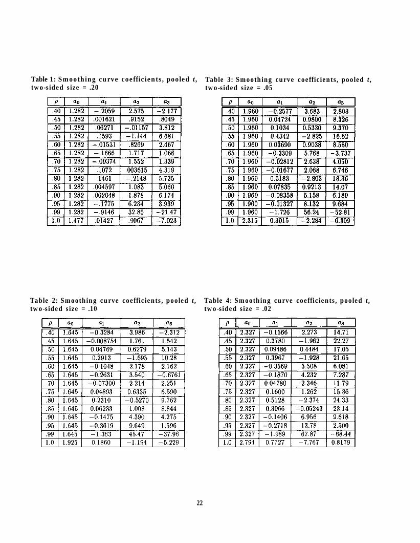
Table 1: Smoothing curve coefficients, pooled t, Table 3: Smoothing curve coefficients, pooled t,two-sided size = .20 two-sided size = .05

Table 2: Smoothing curve coefficients, pooled t, Table 4: Smoothing curve coefficients, pooled t,two-sided size = .10 two-sided size = .02

22

Table 5: Smoothing curve coefficients, pooled t,two-sided size = .01

Table 7: Smoothing curve coefficients, paired t,two-sided size = .10

Table 6: Smoothing curve coefficients, paired t, Table 8: Smoothing curve coefficients, paired t,two-sided size = .20 two-sided size = .05

23

Table 9: Smoothing curve coefficients, paired t, two-sided size = .02

Table 10: Smoothing curve coefficients, paired t, two-sided size = .01

24

Table 11: Monte Carlo critical values, two-sided size = .05

25

Table 12: Quality summary, pooled statistic, smoothed critical values

Table 13: Quality summary, paired statistic, smoothed critical values

26

Table 14: Quality summary, pooled statistic, incorrect t critical values

Table 15: Quality summary, pooled statistic, “correct” t critical values

27

Table 16: Quality summary, paired statistic, “correct” t critical values

28

1For the purposes of the study, “good” means that the actual sizes are below .22, .11, .055, .025, and .0125 forthe nominal .20, .10, .05, .02, and .01 cases. The fact that .005 is 10% of .05 and .005 is 25% of .02 accounts for thenon-monotonic sample sizes.

29

Tab

le 1

9: P

ower

, ρ ρ

= .4

0, s

mal

l n,

nom

inal

siz

e =

.01

Tab

le 1

9 co

ntin

ued:

Pow

er,

ρ ρ = =

.40,

sm

all

n, n

omin

al s

ize

= .0

1

Tab

le 2

0: P

ower

, ρ ρ

=.5

0, s

mal

l n,

nom

inal

siz

e =

.01

33

Tab

le 2

1: P

ower

, ρ ρ

= .6

0, s

mal

l n,

nom

inal

siz

e =

.01

Tab

le

21

con

tin

ued

: P

ower

, ρ ρ

= .6

0, s

mal

l n,

nom

inal

si

ze

=

.01

Tab

le 2

2: P

ower

, ρ ρ

= .7

0, s

mal

l n,

nom

inal

siz

e =

.01

Tab

le 2

2 co

ntin

ued:

Pow

er,

ρ ρ =

.70,

sm

all

n, n

omin

al s

ize

= .0

1

Tab

le 2

3: P

ower

, ρ ρ

= .8

0, s

mal

l n,

nom

inal

siz

e =

.01

Tab

le 2

3 co

ntin

ued:

Pow

er,

ρ ρ =

.80,

sm

all

n, n

omin

al s

ize

= .0

1

Tab

le 2

4: P

ower

, ρ ρ

= .8

5, s

mal

l n,

nom

inal

siz

e =

.01

Tab

le 2

4 co

ntin

ued:

Pow

er,

ρ ρ =

.85,

sm

all

n, n

omin

al s

ize

= .0

1

Tab

le 2

5: P

ower

, ρ ρ

= .9

0, s

mal

l n,

nom

inal

siz

e =

.01

Tab

le 2

5 co

ntin

ued:

Pow

er,

ρ ρ =

.90,

sm

all

n, n

omin

al s

ize

= .0

1

Tab

le 2

6: P

ower

, ρ ρ

=.9

5, s

mal

l n,

nom

inal

siz

e =

.01

Tab

le 2

6 co

ntin

ued:

Pow

er,

ρ ρ =

.95,

sm

all

n, n

omin

al s

ize

= .0

1

Tab

le 2

7: P

ower

, ρ ρ

= .9

9, s

mal

l n,

nom

inal

siz

e =

.01

Tab

le 2

7 co

ntin

ued:

Pow

er,

ρ ρ =

.99,

sm

all

n, n

omin

al s

ize

= .0

1

Tab

le 2

8: P

ower

, ρ ρ

= .4

0, l

arge

n, n

omin

al s

ize

= .0

1

Tab

le 2

8 co

ntin

ued:

Pow

er,

ρ ρ =

.40,

lar

ge n

, nom

inal

siz

e =

.01

Tab

le 2

9: P

ower

, ρρ

= .5

0, l

arge

n, n

omin

al s

ize

= .0

1

Tab

le 2

9 co

ntin

ued:

Pow

er,

ρ ρ =

.50,

lar

ge n

, nom

inal

siz

e =

.01

I

Tab

le 3

0: P

ower

, ρ ρ

= .6

0, l

arge

n,

nom

inal

siz

e =

.01

Tab

le 3

0 co

ntin

ued:

Pow

er,

ρ ρ =

.60,

lar

ge n

, no

min

al s

ize

= .0

1

Tab

le 3

1: P

ower

, ρ ρ

= .7

0, l

arge

n, n

omin

al s

ize

= .0

1

Tab

le 3

1 co

ntin

ued:

Pow

er,

ρ ρ =

.70,

lar

ge n

, nom

inal

siz

e =

.01

Tab

le 3

2: P

ower

, ρ ρ

= .8

0, l

arge

n, n

omin

al s

ize

= .0

1

Tab

le 3

2 co

ntin

ued:

Pow

er,

ρ ρ =

.80,

lar

ge n

, nom

inal

siz

e =

.01

Tab

le 3

3: P

ower

, ρ=

ρ=

.85

, la

rge

n, n

omin

al s

ize

= .0

1

Tab

le 3

3 co

ntin

ued:

Pow

er,

ρ ρ =

.85,

lar

ge n

, nom

inal

siz

e =

.01

Tab

le 3

4: P

ower

, ρ=

ρ=

.90

, la

rge

n, n

omin

al s

ize

= .0

1

Tab

le 3

4 co

ntin

ued:

Pow

er,

ρ ρ =

.90,

lar

ge n

, nom

inal

siz

e =

.01

Tab

le 3

5: P

ower

, ρ ρ

= .9

5, l

arge

n, n

omin

al s

ize

= .0

1

Tab

le 3

5 co

ntin

ued:

Pow

er,

ρ ρ =

.95,

lar

ge n

, nom

inal

siz

e =

.01

Tab

le 3

6: P

ower

, ρ ρ

=.9

9, l

arge

n, n

omin

al s

ize

= .0

1

Tab

le 3

6 co

ntin

ued:

Pow

er,

ρ ρ =

.99,

lar

ge n

, nom

inal

siz

e =

.01

Tab

le 3

7: P

ower

, ρ ρ

= .4

0, s

mal

l n,

nom

inal

siz

e =

.05

Tab

le 3

7 co

ntin

ued:

Pow

er,

ρ ρ =

.40,

sm

all

n, n

omin

al s

ize

= .0

5

Tab

le 3

8: P

ower

, ρ ρ

= .5

0, s

mal

l n,

nom

inal

siz

e =

.05

Tab

le 3

8 co

ntin

ued:

Pow

er,

ρ ρ =

.50,

sm

all

n, n

omin

al s

ize

= .0

5

Tab

le 3

9: P

ower

, ρ ρ

=.6

0, s

mal

l n,

nom

inal

siz

e =

.05

Tab

le 3

9 co

ntin

ued:

Pow

er,

ρ ρ =

.60,

sm

all

n, n

omin

al s

ize

= .0

5

Tab

le 4

0: P

ower

, ρ ρ

=.7

0, s

mal

l n,

nom

inal

siz

e =

.05

Tab

le 4

0 co

ntin

ued:

Pow

er,

ρ ρ =

.70,

sm

all

n, n

omin

al s

ize

= .0

5

Tab

le 4

1: P

ower

, ρ ρ

=.8

0, s

mal

l n,

nom

inal

siz

e =

.05

Tab

le 4

1 co

ntin

ued:

Pow

er,

ρ ρ =

.80,

sm

all

n, n

omin

al s

ize

= .0

5

Tab

le 4

2: P

ower

, ρ ρ

=.8

5, s

mal

l n,

nom

inal

siz

e =

.05

Tab

le 4

2 co

ntin

ued:

Pow

er,

ρ ρ =

.85,

sm

all

n, n

omin

al s

ize

= .0

5

Tab

le 4

3: P

ower

, ρ ρ

=.9

0, s

mal

l n,

nom

inal

siz

e =

.05

Tab

le 4

3 co

ntin

ued:

Pow

er,

ρ ρ =

.90,

sm

all

n, n

omin

al s

ize

= .0

5

Tab

le 4

4: P

ower

, ρ ρ

=.9

5, s

mal

l n,

nom

inal

siz

e =

.05

Tab

le 4

4 co

ntin

ued:

Pow

er,

ρ ρ =

.95,

sm

all

n, n

omin

al s

ize

= .0

5

Tab

le 4

5: P

ower

, ρ ρ

= .9

9, s

mal

l n,

non

inal

siz

e =

.05

Tab

le 4

5 co

ntin

ued:

Pow

er,

ρ ρ =

.99,

sm

all

n, n

omin

al s

ize

= .0

5

Tab

le 4

6: P

ower

, ρ ρ

=.4

0, l

arge

n, n

omin

al s

ize

= .0

5

Tab

le 4

6 co

ntin

ued:

Pow

er,

ρ ρ =

.40,

lar

ge n

, nom

inal

siz

e =

.05

Tab

le 4

7: P

ower

, ρ ρ

=.5

0, l

arge

n, n

omin

al s

ize

= .0

5

Tab

le 4

7 co

ntin

ued:

Pow

er,

ρ ρ =

.50,

lar

ge n

, nom

inal

siz

e =

.05

Tab

le 4

8: P

ower

, ρ ρ

=.6

0, l

arge

n, n

omin

al s

ize

= .0

5

Tab

le 4

8 co

ntin

ued:

Pow

er,

ρ ρ =

.60,

lar

ge n

, nom

inal

siz

e =

.05

Tab

le 4

9 co

ntin

ued:

Pow

er,

ρ ρ =

.70,

lar

ge n

, nom

inal

siz

e =

.05

Tab

le 5

0: P

ower

, ρ ρ

=.8

0, l

arge

n, n

omin

al s

ize

= .0

5

Tab

le 5

0 co

ntin

ued:

Pow

er,

ρ ρ =

.80,

lar

ge n

, nom

inal

siz

e =

.05

Tab

le 5

1: P

ower

, ρ ρ

=.8

5, l

arge

n, n

omin

al s

ize

= .0

5

Tab

le 5

1 co

ntin

ued:

Pow

er,

ρ ρ =

.85,

lar

ge n

, nom

inal

siz

e =

.05

Tab

le 5

2: P

ower

, ρ ρ

= .9

0, l

arge

n, n

omin

al s

ize

= .0

5

Tab

le 5

2 co

ntin

ued

Pow

er,

ρ ρ =

.90,

lar

ge n

, nom

inal

siz

e =

.05

Tab

le 5

3: P

ower

, ρ ρ

= .9

5, l

arge

n, n

omin

al s

ize

= .0

5

Tab

le 5

3 co

ntin

ued:

Pow

er,

ρ ρ =

.95,

lar

ge n

, nom

inal

siz

e =

.05

Tab

le 5

4: P

ower

, ρ ρ

=.9

9, l

arge

n, n

omin

al s

ize

= .0

5

Tab

le 5

4 co

ntin

ued:

Pow

er,

ρ ρ =

.99,

lar

ge n

, nom

inal

siz

e =

.05

Table 55: Power, ρ ρ = .95, n = 24, nominal size = .01, misspecified model

102

Table 56: Example data

103

Table 56 continued: Example data

104

Table 56 continued: Example data

105