PortfolioAllocation ofHedgeFunds - Thierry Roncalli · PortfolioAllocation ... funds portfolio is...

Portfolio Allocationof Hedge Funds∗

Benjamin BruderResearch & Development

Lyxor Asset Management, [email protected]

Serge DarollesResearch & Development


Abdul KoudiratyResearch & Development


Thierry RoncalliResearch & Development


January 2010

Abstract

Research in hedge fund investing proposes different solutions to build optimal hedgefund portfolios. However, these solutions are direct extensions of the usual mean-variance framework, and still suffer from model risks. More complex approaches startto be used but are related to numerous estimation risks. We compare in this paperthe out-sample properties of different allocation models through a dynamic investmentexercise using hedge fund indices. We show that the best out-of-sample properties areobtained by allocation models that take into account the specific statistical propertiesof hedge fund returns.

Keywords: Hedge funds, portfolio allocation, higher-order moments, regime-switchingmodels.

JEL classification: G11, G24, C53.

1 IntroductionHedge fund returns differ substantially from the returns of standard asset classes, makinghedge funds of interest to investors seeking to diversify balanced portfolios. Research intohedge fund investing has therefore naturally focused on finding the optimal proportion inwhich to invest in hedge funds1, measuring hedge fund performance2, identifying hedge fundrisk factors3, and finally constructing optimal hedge fund portfolios4. However, despite the

∗We are grateful to L. Erdely, J.M. Stenger and G. Comissiong for their helpful comments.1see e.g. Terhaar et al. (2003), Cvitanic et al. (2003), Popova et al. (2003), Amin and Kat (2003).2see e.g. Eling and Schumacher (2007), Darolles et al. (2009), Darolles and Gourieroux (2010).3see e.g. Fung and Hsieh (1997), Ackermann et al. (1999), Brown et al. (1999), Liew (2003), Agarwal

and Naik (2004), Agarwal et al. (2009), Buraschi et al. (2010), Darolles and Mero (2010).4see e.g. Amenc and Martellini (2002), McFall Lamm (2003), Kat (2004), Agarwal and Naik (2004),

Alexander and Dimitriu (2004), Morton et al. (2006), Giomouridis and Vrontos (2007), Adam et al. (2008).

PORTFOLIO ALLOCATION OF HEDGE FUNDS

nature of hedge fund investments (dynamic trading strategies, use of derivatives and lever-age) and their observable consequences on hedge fund return characteristics (time-varyingcovariance parameters, high kurtosis of returns distributions), this research is mainly con-ducted in the usual framework of normal independent and identically distributed (i.i.d.)returns. For example, Giomouridis and Vrontos (2007) are the first to use dynamic spec-ification for the covariance parameters and to evaluate the consequences at the portfolioallocation level. More generally, we can think that the standard methods used for portfolioallocation are inadequate since non null skewness and high kurtosis, relative to traditionalasset classes, are observed in the monthly returns of hedge funds5.

The mean-variance approach (Markovitz, 1952) is a standard in the asset management in-dustry. This approach is founded on the assumption of normal i.i.d. returns and is naturallysubject to criticisms, when applied to build portfolios involving hedge funds. These criti-cisms stress that mean-variance is in this case only appropriate for investors having quadraticpreferences, thus making it not applicable in all situations. But this kind of analysis is widelyused in practice as well as in the literature. Among others, Amenc and Martellini (2002),Terhaar et al. (2003) and Alexander and Dimitriu (2004) consider hedge fund allocationin this framework. However, alternative approaches have already been proposed. Bares etal. (2002) and Cvitanic et al. (2003) compute optimal portfolios in an expected utilityframework. Amin and Kat (2003) discuss the problems arising in mean-variance allocationwhen the asset returns are not symmetric. Popova et al. (2003), Hagelin and Pramborg(2003), Jurczenko et al. (2005) and Davies et al. (2009) introduce higher moments analysis.Krokhmal et al. (2002), Favre and Galeano (2002), Agarwal and Naik (2004) and Adam etal. (2008) construct optimal portfolios using alternative risk measures. Given the increasinginterest for risk management, there is indeed a multiplication of measures capturing differenttypes of risks and several tentatives to unify these approaches. Rockafellar et al. (2006) forexample propose generalized measures as substitutes for volatility.

In this paper, we consider a general set of asset allocation models to measure the dif-ferences in allocation obtained when using alternative specifications. We first consider themean-variance model and then discuss basic extensions that do not involve expected returnestimation and are presumed to be more robust against estimation errors. Such extensionsinclude the minimum-variance (Clarke et al., 2006), constant-Sharpe (Martellini, 2008),equally-weighted risk contribution (Maillard et al., 2010) and most diversified (Choueifatyand Coignard, 2008) portfolios. We also consider optimal portfolios as determined by maxi-mizing different utility functions and the Omega ratio risk measure. Each of these approachesis given a set of solutions that can be easily compared when applied to hedge fund returns.We then examine four extensions that seem particularly promising in addressing the appro-priate allocation to hedge funds. First, we include higher-order moments in the objectivefunction to maximize. This extension allows investors to recognize and use information em-bedded in the unusual distribution of hedge fund returns (Martellini and Ziemann, 2010).Second, we address the issue of time-varying variance covariance parameters and their po-tential impact on hedge fund portfolio allocation. We use the regime-switching dynamiccorrelation model6 to include these stylized facts in the covariance matrix specification.Third, we include exogenous stress scenarios to reflect the possibility of extreme drawdownsattributable to certain rare events. Fourth, we consider the impact of inclusion of managers’views of portfolio performance in a Black-Litterman framework.

5see e.g. Fung and Hsieh (1997, 2001), Brooks and Kat (2002), Popova et al. (2003), Agarwal and Naik(2004), Martellini and Ziemann (2010).

6see, e.g. Pelletier (2006), Giomouridis and Vrontos (2007).

2


To evaluate the models ability to work with non-normal distribution and time-varyingparameters, we illustrate our analysis by actively managing a fund of hedge funds invested inhedge fund indices from the CSFB/Tremont and HFR database. We use index data insteadof single hedge fund data for essentially two reasons. First, the direct optimization of a hedgefunds portfolio is impossible with regards to the variety of investment constraints relatedto each individual hedge fund. This explains why portfolio construction is in practice donein two steps. The first step corresponds to strategic and tactical allocation and determinesthe portfolio profile in terms of strategies. The second step is the implementation of thedecision allocation, with the choice of specific hedge funds allowing the portfolio managerto implement the strategic/tactical allocation bets. As this second step necessarily involvesdeep qualitative analysis of each candidate hedge fund, quantitative models are more relevantduring the first step, i.e. when allocating between hedge fund strategies. Second, Darollesand Vaissie (2010) find that the added value of funds of hedge funds at the tactical level ispoor. It is then of great interest to evaluate quantitative allocation tools to actively managethe tactical allocation of hedge fund portfolios and enhance the total added value proposedby funds of hedge funds. The paper is organized as follow. Section 2 describes the classicallocation models used as benchmarks for our analysis. Section 3 presents two allocationmodels developed in the particular context of hedge funds portfolio construction. Section 4applies benchmark and specific models to hedge fund data. Finally, Section 5 concludes.

2 Models of portfolio optimization

In what follows, we describe the different models that can be used to determinate theportfolio allocation of hedge funds. We consider a universe of n hedge fund strategies. Wedenote by Ri,t the return of the ith strategy at time t. µ and Σ are the expected return andthe covariance matrix of the returns (R1,t, . . . , Rn,t). Let w be the weights of the portfolio.We suppose that the portfolio construction faces some constraints and we note w ∈ A. Forexample, we may assume that the weights are positive and sum to one. In this case, A isthe simplex set:

A =

x ∈ [0, 1]n :

n∑

i=1

xi = 1

In order to be more legible, we do not report the constraints w ∈ A in the optimizationprograms, but they are taken into account implicitly.

2.1 Mean-variance framework

2.1.1 Optimization program

The mean-variance framework was introduced by Markowitz (1952) and is now widely used.The main idea of that seminal work is to find an efficient equilibrium between risks andreturns. More precisely, the market risks are entirely monitored by the variance of theportfolio while the returns are characterized through their expected value. Its popularitycomes from the fact that this program produces an optimal allocation with respect to anyrisk-averse criterion based on probabilities, as long as the asset return distributions aresupposed to be gaussian. Indeed, in that case, any portfolio has a gaussian behavior, whichis therefore completely described by its return and its variance. On the other hand, manystudies (see e.g. Cont, 2001) show that asset returns are not normally distributed, especiallywhen considering hedge funds (Fung and Hsieh, 1999, Malkiel and Saha, 2005). Hence,considering only the variance as a measure of risks may be insufficient.

3


For any risk-averse investor, the expected return of the portfolio should be maximized,while risk should be minimized. Thus, it is natural to maximize expected returns whilekeeping variance under a given acceptable level:

maxw>µ u.c. w>Σw ≤ σ2max (1)

where w>µ is the expected return of the portfolio and w>Σw denotes the variance of theportfolio. Another equivalent procedure is to minimize the variance while keeping the ex-pected returns above a minimal level:

min w>Σw u.c. w>µ ≥ µmin (2)

Portfolio allocations given by those programs define the mean/variance efficient frontier,that is also the maximal attainable expected return for a given level of risk7.

Another equivalent point of view is to set the following optimization problem:

maxw>µ− λ

2w>Σw (3)

where λ is called the risk aversion parameter. It is clear that the solution of this problemwill maximize expected returns while minimizing portfolio variance. Each parameter λ > 0involves an optimal portfolio corresponding to a given value of µmin in problem (2). Unfortu-nately, the correspondence between the risk aversion parameter λ and the resulting averagereturn µmin can only be found by solving problem (3). Nevertheless, with this formulation,this method could be seen as a special case of utility maximization involving a quadraticutility function8.

2.1.2 Parameter uncertainty problem

The major issue of the mean-variance framework is the estimation of the asset returnscovariance matrix Σ and of the expected returns µ. These parameters can be estimatedwith their empirical counterparts. However, we should emphasize that optimizing the mean-variance criterion through backtesting or with the empirical moments lead exactly to thesame results.

The empirical estimator Σ is traditionally used for the covariance matrix, due to itsappealing properties. Indeed, it corresponds to the maximum likelihood estimator. However,its convergence is very slow especially when the number of assets is large. In this case, Σintroduces some extreme errors, and any optimization procedure will focus on those errors,thus placing big bets on the mostly unreliable coefficients (Michaud, 1989). Shrinkagemethods is a popular solution to obtain a biased but robust covariance matrix.

Let Φ be a biased estimate of Σ. We assume that it converges faster than Σ. In thiscase, we define Σα as a convex combination of these two estimators:

Σα = αΦ + (1− α) Σ

The main problem is to compute the optimal value of α. Ledoit and Wolf (2003) considerthe quadratic loss function L (α) defined as follows:

L (α) =∥∥∥αΦ + (1− α) Σ− Σ

∥∥∥2

7This frontier can be obtained by computing the minimal attainable variance w>Σw for all the expectedreturn level constraints µmin.

8See Section 2.2 for details.

4


They define the optimal value as the solution of the problem α? = arg minE [L (α)]. Ledoitand Wolf (2003) give the analytical solution of α? in the case of a one-factor model, whereasthe optimal estimate α? in the case of a constant correlation matrix may be found in Ledoitand Wolf (2004).

2.1.3 Risk based portfolios

One of the issues of parameter uncertainty is to estimate the expected returns µ. Merton(1980) points that historical estimates fail to account for the effects of changes in the level ofmarket risk and expected returns may be estimated using equilibrium models. Nevertheless,this approach makes sense only for traditional asset classes. In the case of hedge funds, anequilibrium model to estimate the risk premium of one strategy does not exist. That is whywe may prefer to use some allocation methods which are presumed to be more robust asthey are not dependent on expected returns.

The minimum-variance portfolio is the only portfolio on the mean-variance frontier whichdoes not depend on expected returns. More formally, it is defined by the following optimiza-tion program:

w? = arg min w>Σw

This approach is widely used by practitioners (Clarke et al., 2006). However, it may suffersome drawbacks concerning the concentration.

In order to obtain a more diversified portfolio, Maillard et al. (2010) propose to usethe equally-weighted risk contribution portfolio (known as the ERC portfolio). Let σ (w) =√

w>Σw be the volatility of the portfolio. We have:

σ (w) =n∑

i=1

RCi =n∑

i=1

wi∂ σ (w)∂ wi

RCi = wi × ∂wi σ (w) is the risk contribution of the ith strategy to the portfolio volatility.The ERC portfolio corresponds to the portfolio where all the risk contributions are the same:

RCi = RCj

As shown by Maillard et al. (2010), the ERC portfolio may be viewed as a minimum-varianceportfolio subject to a constraint of sufficient diversification in terms of weights.

In the third approach, we assume that the risk premium is proportional to the volatility.It means that all components of the portfolio have the same Sharpe ratio s. The Sharperatio of the portfolio is defined by:

sh (w) =w> (µ− r)√

w>Σw= s

w>σ√w>Σw

Maximizing the Sharpe ratio is then equivalent to maximizing the dispersion ratio. Thisportfolio is known as the most diversified portfolio (Choueifaty and Coignard, 2008).

5


2.2 Utility theory

2.2.1 General framework

The utility function framework was introduced by Von Neumann and Morgenstern (1953)and has been widely used since by academics and practitioners to handle portfolio manage-ment problems. This theory states that, under some assumptions, the investor’s preferencein terms of returns distributions can be ordered with the expected value of a utility function.That is, an allocation is preferred to another if the expected utility of the resulting wealthat some fixed time T is higher. In mathematical terms, a portfolio w1 resulting in somerandom wealth W

(w1)T at time T is preferred to w2 leading to W

(w2)T if:

E[U

(W

(w1)T

)]> E

[U

(W

(w2)T

)]

We can interpret U (x) as the “satisfaction” of the investor to possess the wealth level x.Therefore, we must find the portfolio that achieves a maximum expectation of the utilityfunction.

As described in Appendix A.2, this criterion features both appetite for gains and riskaversion. Of course, even if we suppose that the probability distribution of assets returnsis perfectly known, we must specify the utility function for our problem. This is the majorweakness of this kind of framework. Indeed, two difficulties appear. First of all, this utilityfunction should be different for every investor, thus introducing difficulties in fund manage-ment. Second, the utility function of an investor is very difficult to formalize, and there isno clear method to build it. Nevertheless, in Appendix A.2 we come up with some intuitionson the behavior of utility functions and provide some fundamental examples.

2.2.2 Application to the empirical distribution

Let us consider the utility maximization problem. Once the utility function has been fixed,the main difficulty is to estimate the joint probability distribution of the asset returns. Ifwe consider a gaussian distribution, the utility problem is strictly equivalent to the mean-variance problem. Indeed, with such assumptions, the returns of any portfolio is gaussianand is entirely characterized by its mean and variance parameters. Therefore, as the utilityfunction introduces a risk adverse behavior together with an appetite for gains, the programconsist in maximizing the average return while minimizing the volatility of the portfolio.This is equivalent to solving the optimization program (3). A non-gaussian probabilitydistribution leads to a different optimal portfolio. Therefore, this choice is crucial. Thisproblem is avoided by using the empirical distribution of the asset returns, i.e. maximizingthe expected utility function through backtesting (Sharpe, 2007).

All allocations w are first backtested, leading to the historical monthly performance rwt

of all corresponding portfolios. These backtests are then used to compute the historicalutility of the corresponding portfolio as follows:

U (w) =1n

n∑t=1

u (1 + rwt )

In the last step, we maximize the historical average utility function to find out the portfolioweights w? such that:

w? = arg max U (w)

6


This method can be interpreted as a “ let the data talk ” approach. No explicit statisticalmodel assumptions are needed, and model risk is irrelevant. We only introduce assumptionabout the preferences of the investor (i.e. the utility function).

2.3 Omega ratio

2.3.1 Definition

The Omega ratio performance measure was introduced in Shadwick and Keating (2002).Let F be the cumulative distribution function of the portfolio returns. For a given thresholdH, the Omega ratio is defined as follows:

Ω(H) =

∫ +∞H

(1− F (x)) dx∫ H

−∞F (x) (x) dx

It can be also written as9:

Ω(H) =Pr R > H × E [R−H | R > H]Pr R < H × E [R−H | R < H]

Therefore, it can be interpreted as the ratio between the average returns above H and theaverage returns below H (or call-put ratio). If H = 0, it is the ratio between average gainsand losses, weighted by the probabilities of those events. Therefore, H can be interpreted asthe threshold above which a return is considered as a gain and below which the returns areconsidered as losses. An order of magnitude of Ω can be derived by remarking that settingthe threshold H equal to the mean return E [R] of the portfolio leads to an Omega ratioequal to 1. In other words, Ω(E [R]) = 1 for any portfolio.

Let Ω? (H) be the optimal portfolio Omega ratio. Maximizing the Omega ratio for agiven value H is equivalent to maximizing the following utility function:

U (x) = (x−H)+ − Ω? (H) (H − x)+= x−H + (1− Ω? (H)) (H − x)+

When the optimal Omega ratio Ω? (H) is below 1, the utility function is convex, while anoptimal ratio Ω? (H) above 1 corresponds to a concave utility function. The behavior of theinvestor is risk adverse when Ω? (H) > 1, while it is risk-seeking when Ω? (H) < 1. Lastly,an Omega ratio equal to 1 induces a risk-neutral behavior. When Ω? (H) < 1, the riskseeking behavior is not conventional as an investor will try to maximize his risk for a givenexpected return level. Therefore, allocation based on the Omega ratio is misleading andinaccurate when Ω? (H) < 1. This can be considered together with the property that theOmega ratio is equal to 1 when the target H is equal to the mean return of the portfolio.To conclude, the target H should be set carefully, ensuring that this performance level His attainable on average by some portfolios based on available assets. For example, this isalways the case if H is the return of the riskless asset.

9Let f be the density function of F. We have:

Ω(H) =

R+∞H

R+∞x f (y) dy dx

RH−∞

R x−∞ f (y) dy dx

=

R+∞H (x−H) f (x) dxRH−∞ (H − x) f (x) dx

=Eh(X −H)+

i

Eh(H −X)+

i

7


2.3.2 Regularization of the Omega ratio using the Cornish-Fisher expansion

As in the case of utility maximization, the empirical distribution can be used to optimize theOmega ratio. However, this is a difficult task, as standard maximization procedures tendto perform poorly. Furthermore, as we use a limited set of returns (typically 24 monthlyreturns), there often exists an asset that never performs below the threshold H, thus leadingto an infinite Omega ratio. This problem gets even worse when several assets exhibit thisbehavior, as any combination of these assets lead to an infinite Omega ratio, and the optimalallocation cannot be uniquely defined. Thus, we need a smoother criterion that takes intoaccount the possibility of losses in any case. To this end, we introduce the Cornish-Fisherapproximation of the empirical distribution of the portfolio. We compute the four firstmoments of the returns of every allocation we consider. These moments characterize thedistribution of returns. The Cornish Fisher approximation takes those moments as an inputto build a distribution, which we use to calculate the past Omega ratio of the consideredportfolio. We do not consider the moments and distribution of each asset separately, butonly the moments of the historical performance obtained by each portfolio constructed withthose assets. Therefore, we do not need to consider explicitly the assets covariances, orhigher order cross-moments, which may be poorly estimated. Details are given in AppendixA.3.

3 Hedge Funds portfolio specific models

There is a trade-off between model risk and estimation risk in the choice of an allocationmodel (see, e.g. Amenc and Martellini, 2002, in the case of hedge funds investing). If themodel is simple, then the risk to miss some important characteristics of the return distri-bution is high. But this kind of model is likely to be more robust and associated withsmall estimation errors. On the contrary, the use of a more sophisticated model in generaldecreases the model risk, but also increases dramatically the estimation risk and generatesrobustness issues. The literature of hedge funds investing addresses this issue and proposestwo extensions of the usual mean-variance framework that take into account the estimationrisk dimension. The first extension starts from the expected utility maximization approach,but use finite dimension approximation of the utility function to first reduce the problemdimension, and then impose some structure on the covariance and higher-order comoments(Martellini and Ziemann, 2010). The second extension involves more complex specificationsof the covariance matrix that is the central parameter driving portfolio allocation. A parsi-monious dynamic specification of these covariance parameters are proposed in Giomouridisand Vrontos (2007).

3.1 Taking into account higher-order moments

A way to reduce model risk is to consider higher comoments, i.e. coskewness and cokurtosis,in addition to covariance. However, this approach increases further the estimation risk whichis already high in the classic mean-variance framework when the number of assets is high.Therefore, one could wonder whether the framework using higher-order moments could beimplemented in a realistic way. Martellini and Ziemann (2010) apply some statistical tech-niques already used in the mean-variance framework to higher-order moments estimation.These extensions are dimension reduction techniques based on constant correlation (Eltonand Gruber, 1973) and single-factor based (Sharpe, 1963) estimators.

8


3.1.1 Finite dimensional expansion

To account for the impact of higher-order moments of asset returns on the portfolio alloca-tion, Martellini and Ziemann (2010) consider the finite dimensional expansion of a standardexpected utility maximization framework introduced in Section 2.2. Assuming infinite dif-ferentiability, the utility function U can be approximated as follows:

U (W ) =∞∑

k=0

Uk (E [W ])k!

(W − E [W ])k

where W is a random variable representing investor’s terminal wealth. One can typicallyassume that the fourth-order development is sufficient to get a good approximation. Wecut the sum after the fourth term and apply the expectation operator to both sides of theprevious equation. We then get the approximated expected utility:

E [U (W )] ' U (E [W ]) +12U (2) (E [W ]) µ(2) +

16U (3) (E [W ]) µ(3) +

124

U (4) (E [W ]) µ(4)

where µ(n) = E [W − E [W ]]n denotes the nth-order centered moment of W . Thus, maximiz-ing this approximated expected utility allows investors to account for first, second, but alsothird (skewness) and fourth (kurtosis) moments and comoments of the underlying assets inthe portfolio. Portfolio choice is no longer a trade-off between expected return and volatilityas in the mean-variance case. It involves high moments considerations that can be writtenas direct functions of portfolio weights.

To get an explicit form of the higher-order moments and comoments, Martellini andZiemann (2010) introduce higher-order moment tensors M2, M3 and M4 (see Jondeau andRockinger, 2006 and Appendix A.4 for explicit expressions of these tensors). As in the gen-eral expected utility maximization framework, we choose a given U to completely specifythe objective function. We use in the following a CARA utility function. More gener-ally, this approach can be seen as a midpoint between the mean-variance and the expectedutility maximization framework. Indeed, the two-order approximation corresponds to themean-variance case, as the limiting case is the expected utility maximization case. Thissuggests applying covariance cleaning techniques developed in the mean-variance case tomore complex allocation models.

3.1.2 Taking into account estimation risk

Even in the mean-variance case, the number of parameters to estimate increases dramati-cally with the number of assets. This problem is of course even more important when weconsider higher-order moments. For an illustration, we develop the example of n = 10 as-sets. The number parameters involved in M2 (respectively M3 and M4) is 55 (respectively220 and 715). Martellini and Ziemann (2010) then address the dimension reduction issuewhen estimating the M2, M3 and M4 tensors. Two improved estimators for the higher-ordermoment tensor matrices are proposed. The constant correlation estimator (Elton and Gru-ber, 1973) is a classic solution to overcome the covariance matrix estimator for portfolioscontaining a large number of assets. A constant correlation across the underlying assetsimproves the out-of-sample mean-variance portfolio performance despite the specificationerror. Martellini and Ziemann (2010) extend this approach to M3 and M4 estimators.

An unbiased estimator for the constant correlation parameter is given by the average of

9


all sample correlation parameters:

ρ =2

N(N − 1)

∑

i<j

Σi,j√Σi,iΣj,j

where Σi,j denotes the sample covariance between assets i and j. Thus, the covariancecoefficient can be estimated as follows:

σi,j = ρ

√Σi,iΣj,j

Martellini and Ziemann (2010) extend the idea of constant correlation to the context ofhigher-order moment tensors by including appropriate combinations of higher-order como-ments according to the definition of the matrices M3 and M4.

The single-factor based estimator (Sharpe, 1963) assumes that a single factor explain then individual asset returns:

Ri,t = c + βiFt + εi,t

where Ft is a well-diversified market index at time t and εi,t is the idiosyncratic error termof asset i. The regression residual are assumed to be homoscedastic and cross-sectionallyuncorrelated with covariance matrix Ψ. Based on this specification, the elements of thecovariance matrix and the higher-order moment tensors have the following forms:

M2 = ββ>µ(2)0 + Ψ

M3 = (ββ> ⊗ β>)µ(3)0 + Φ

M4 = (ββ> ⊗ β> ⊗ β>)µ(4)0 + Γ

where µ(2)0 , µ

(3)0 and µ

(4)0 are respectively the second, third and fourth centered moments of

the single factor and ⊗ designates the tensor product between two matrices. The detailedformulas of Φ, Ψ and Γ are provided in Martellini and Ziemann (2010).

3.2 Regime-switching dynamic correlation modelAs our focus on hedge funds is portfolio allocation, it is natural to discuss the specification ofthe covariance matrix, the essential input of the mean-variance approach. Empirical evidenceobserved on hedge fund returns exclude static specifications and clearly support the use ofdynamic models. There are numerous dynamic specifications but, following Giomouridisand Vrontos (2007), we consider regime-switching models for two reasons. First, they showthat this approach is the most relevant to model hedge fund data. Second, we can controlthe increase in the number of parameters by limiting the number of states.

The notion of regime-switching models for correlation was introduced by Ang and Chen(2002) for explaining asymmetry in the correlation of an equity portfolio. This kind ofstylized facts is also observed on hedge fund returns during the last subprime crisis, wherecorrelations where submitted to brutal changes. Therefore, a model in which the correlationcould switch between states of nature should be able to provide a better explanation ofthe asset’s joint behavior. Intuitively, this switching approach can be seen as a midpointbetween the constant correlation coefficient (Bollerslev, 1990) and the dynamic correlationcoefficient (Engle 2002) models. The first model assumes constant correlation over time. Thesecond allows correlations to change at every period. In the switching approach, correlation

10


can only take a finite number of values. We use the dynamic specification proposed byPelletier (2006) and applied to hedge fund allocation problem by Giomouridis and Vrontos(2007). More generally, regime-switching models are used in the hedge funds literature ina number of contexts including measuring the systemic risk (Chan et al., 2006, Billio etal., 2010), studying serial correlations (Getmansky et al., 2004) and detecting switchingstrategies (Alexander and Dimitiu, 2004).

In this section we provide a short presentation of the regime-switching dynamic correla-tion (RSDC hereafter). The hedge fund returns are defined by:

Rt = µ + εt

where εt|It−1 ∼ N (0, Vt), µ is a n×1 vector of constants, εt is a n×1 innovation vector andIt is the information available up to time t. The n× n covariance matrix Vt is decomposedinto:

Vt = ΣtCtΣt

where Σt is a diagonal matrix composed of the standard deviations σi,t (i = 1, . . . , n) andCt is the correlation matrix. Both matrices are time-varying. In particular, the conditionalvariances σi,t are modeled using a GARCH(1,1) specification of the form:

σ2i,t = αi + βiε

2i,t + γiσ

2i,t−1

while the correlation matrix Ct is modeled in a dynamic framework by using:

Ct =K∑

k=1

1 St = k · Ck

where 1 is the indicator function, St is an unobserved Markov chain process independent ofεt which can take K possible values (St = 1, 2, ...,K) and Ck are correlation matrices withCk 6= Ck′ for k 6= k′. Regime switches in the state variable St are assumed to be governedby the transition probability matrix Π = (πi,j). The transition probabilities between statesfollow a first order Markov chain:

Pr St = j|St−1 = i, St−2 = k, . . . = Pr St = j|St−1 = i = πi,j

As in Pelletier (2006) and Giomouridis and Vrontos (2007), we assume that K = 2. Theestimation of the RSDC model can be achieved by using a two-steps procedure (Engle, 2002).In the first step, we estimate the univariate GARCH model parameters. In the second step,we estimate the parameters in the correlation matrix and the transition probabilities πi,j

conditional on the first step estimates. Details of the estimation procedure can be found inPelletier (2006).

3.3 Taking into account stress scenariosHedge fund returns exhibit negative skewness and positive excess kurtosis. These mathe-matical properties can be explained through the exposure of these funds to extreme events.Indeed, hedge fund returns show stable positive returns with little volatility most of thetime, but may experience severe drawdowns on rare occasions, with a magnitude exceedingseveral times their usual standard deviation. Furthermore, these rare events might not beobserved on historical data. Finding a parametric law that matches this behavior is difficult,as the scope of such probability distributions is huge, and involve a precise knowledge ofevents that typically never happen.

11


The stress testing methodology precisely addresses this question (Berkowitz, 2000). Itintroduces changes in the asset simulation method, such as simulating shocks that occurmore likely than historical observation suggests, or introducing shocks that never happened,to reflect a potential structural change or a major crisis. Therefore, we consider a generic andintuitive method, with the introduction of stress scenarios into the previously used probabil-ity distribution. This framework can be applied to any parametric or empirical distribution,as well as in the mean-variance framework. We add to the probability distribution of assetreturns a set of scenarios that may happen with a given probability (see Appendix A.5 fordetails).

3.4 How to incorporate the manager’s views?

The classical method to incorporate the manager’s view is to use the Black-Litterman (BL)method described in Appendix A.6. Given a reference portfolio, the idea of this model isto modify the allocation in order to take into account the views of the manager. It may beviewed as a model of tactical asset allocation.

The BL portfolio is a weighted average of the reference portfolio w0 and the portfolio w?

reflecting the views of the manager:

w = αw0 + (1− α)w?

One difficulty is to define the weight α. Generally, one considers a tracking error constraintto compute α. The input of the model is the value and the uncertainty of the views. Wehave:

Pµ = Q + ε

with ε ∼ N (0, Ω). Suppose for example that the manager thinks that the second strategywill outperform the first strategy by 3% in mean and that the expected return of the thirdstrategy will be 10%. We then have:

( −1 1 00 0 1

)

µ1

µ2

µ3

=

(3%10%

)+

(ε1

ε2

)

Now, he has to define the uncertainty of his views. This is done by scenario analysis. Forexample, if he think that Pr µ2 > µ1 + x% = y%, we deduce that the volatility of ε1 is(x%− 3%)/Φ−1 (1− y%). For example, if the manager thinks that the probability thatthe second strategy will outperform the first strategy by 5% is 20%, the uncertainty or thevolatility of ε1 is 2.54%.

4 Empirical Results

4.1 Data

We illustrate our analysis by constructing an actively managed fund of funds investing inhedge fund indices from the CSFB/Tremont database. CSFB/Tremont computes monthlyreturn data for the 10 strategy indices: convertible arbitrage (CA), dedicated short bias(SB), emerging markets (EM), equity market neutral (EMN), event driven (ED), fixed in-come arbitrage (FI), global macro (GM), long/short equity (LS), managed futures (MF) and

12


multi-strategy (MS). CSFB/Tremont also publish a global index (CST Index) that corre-sponds to an asset-weighted average of all strategy index performances, with some additionalconcentration risk limit. The returns cover the time period from January 1994 through May2010 for a total of 197 monthly returns. It includes a number of crises that occurred inthe 1990s, i.e. the Mexican, Asian, Russian, LTCM crises as well as the IT bubble in 2000and the subprime crisis in 2008. This last crisis is particularly interesting since hedge fundperformances during this crisis are disappointing and surprisingly correlated. Figure 1 plotsthe historical evolution of the 10 strategy indices compared to the global index and showsthat this last crisis has a huge impact on most hedge fund strategies.

Figure 1: CSFB/Tremont strategy indices

Table 1 reports summary statistics for the hedge fund indices returns over the period. Itpresents the annualized return, annualized volatility, Sharpe ratio, skewness, kurtosis, his-torical drawdown period (MaxDD), with additional information of the first and last monthcorresponding to this period (Start MDD and End MDD, respectively). The returns of the10 hedge fund strategies are very heterogeneous in terms of risk profile. Some strategieshave relatively high annualized volatilities, such as dedicated short bias, emerging markets,long/short equity and managed futures and can be considered as equity type investments. Onthe contrary, convertible arbitrage, event driven, fixed income arbitrage and multi-strategyexhibit low volatility levels and could be used in a portfolio to substitute some percentageof the fixed income holdings. Differences in the higher-order moments are also important.The kurtosis of the 10 indices returns ranges from 0.07 (managed futures) to 156.44 (eq-uity market neutral), indicating fat-tailness in the return distributions of some strategies,in particular the ones related to arbitrage trading. Concerning the skewness, 5 strategieshave null or slightly positive asymmetry (dedicated short bias, emerging markets, globalmacro, long/short equity and managed futures, i.e. directional strategies). The 5 remain-ing strategies exhibit significant negative asymmetry (convertible arbitrage, equity market

13


neutral, even driven, fixed income arbitrage and multi-strategy, i.e. essentially arbitragetrading strategies). Finally, we observe that the strategies do not produce their historicaldrawdown during the same period. If the subprime crisis is the most difficult period for 6strategies (convertible arbitrage, equity market neutral, even driven, fixed income arbitrage,long/short equity and multistrategy), global macro and emerging markets hit their draw-down in 1998 and managed futures in 1995. Interestingly, the last crisis allows the dedicatedshort bias strategy to end its drawdown period.

Table 1: CSFB/Tremont single strategy indices descriptive statistics

Hedge Funds strategy Ann. Ret Ann. Vol Skew Kurtosis Max DD Start MDD End MDD

Convertible arbitrage 7.65% 7.18% -2.72 15.70 -32.86% Oct-07 Dec-08

Dedicated short bias -2.92% 16.92% 0.75 1.62 -53.54% Aug-98 Apr-10

Emerging markets 7.76% 15.43% -0.76 4.85 -45.15% Jul-97 Jan-99

Equity market neutral 5.10% 10.75% -11.86 156.44 -45.11% Jun-08 Feb-09

Event driven 10.20% 6.09% -2.55 13.86 -19.15% Oct-07 Feb-09

Fixed income arbitrage 4.98% 6.02% -4.25 28.06 -29.03% Jan-08 Dec-08

Global macro 12.32% 10.18% -0.02 3.40 -26.78 % Jul-98 Sep-99

Long/short equity 9.95% 10.02% 0.00 3.53 -21.97 % Oct-07 Feb-09

Managed futures 6.12% 11.79% 0.02 0.07 -17.74 % Mar-95 Nov-95

Multi-strategy 7.89% 5.45% -1.78 6.29 -24.75 % Oct-07 Dec-08

Table 2 reports correlation coefficients computed for the CSFB/Tremont strategy indexreturns. Index returns exhibit low to medium absolute pairwise correlation. Indeed, corre-lations range from a minimum of 6% between managed futures and long short equity, to amaximum of 78% for fixed income and convertible arbitrage. The average pairwise corre-lation is 22%. These low correlations indicate that the potential for risk diversification inhedge fund investment portfolios is high. However, high kurtosis observed in hedge fundreturns suggests the analysis of covariance dynamics. Figure 2 plots the 24−months rollingpairwise correlation analysis and clearly reveals the time-variation behavior of correlations.We observe that pairwise correlations vary over time suggesting that modeling time-varyingcorrelations may improve optimal portfolio construction.

4.2 Traditional allocation approaches

In this section, we present the results of an investment exercise which compares the empiricalout-of-sample performance of the 8 benchmark allocation models introduced in Section 2,i.e. mean-variance (MV), constant-Sharpe (CS), minimum-variance (MIN), equally-weightedrisk contribution (ERC), most diversified portfolio (MDP), the two CARA and CRRA op-timal portfolios (CARA & CRRA) and finally the portfolio obtained when maximizing the

14


Table 2: CSFB/Tremont single strategy indices correlations

(1) (2) (3) (4) (5) (6) (7) (8) (9) (10)

Convertible arbitrage (1) 1.00

Dedicated short bias (2) -0.26 1.00

Emerging markets (3) 0.43 -0.54 1.00

Equity market neutral (4) 0.21 -0.13 0.14 1.00

Event driven (5) 0.66 -0.57 0.70 0.30 1.00

Fixed income arbitrage (6) 0.78 -0.20 0.41 0.32 0.55 1.00

Global macro (7) 0.34 -0.12 0.45 0.07 0.41 0.40 1.00

Long/short equity (8) 0.44 -0.68 0.65 0.19 0.72 0.38 0.46 1.00

Managed futures (9) -0.09 0.09 -0.04 0.00 -0.06 -0.07 0.28 0.06 1.00

Multi-strategy (10) 0.70 -0.19 0.26 0.35 0.52 0.63 0.26 0.42 0.04 1.00

Figure 2: CSFB/Tremont strategy index rolling correlations

15


Figure 3: Density of the correlation variations

Omega ratio (OMEGA). For the mean-variance and constant-Sharpe problems, the volatil-ity target is set to 7% by year. This value is also used to calibrate the parameters of the twoutility functions CARA and CRRA. We also include in our analysis the portfolio investedin the global index and the equal-weighted portfolio. The setup of our experiments is thefollowing. We use the first 24 months history of data to calibrate the empirical distributionor the model parameters. We then construct optimal hedge fund portfolios. Given the op-timized weights, we calculate buy-and-hold returns on the portfolio for a holding period of1 month, at the end of which the estimation and optimization procedures are repeated onthe last 24 months until the end of the dataset. This exercise produces 173 out-of-sampleobservations that cover the period January 1996-May 2010.

First, we examine the realized returns of the constructed portfolios. Given the fundweights wt = (w1,t, w2,t, ..., w10,t) at time t and the realized returns of the 10 indices attime t + 1, the realized return Rp,t+1 of the portfolio at time t + 1 is computed. Figure4 report the backtests of these realized returns for the benchmark models. We analyzethe portfolios performance both before and during the subprime crisis. The 10 backtestedportfolios exhibit very heterogeneous performance and risk profiles. Mean-variance, CARAand CRRA are the most aggressive portfolios, with high positive returns during the firstsubperiod. However, these three portfolios suffer during the last period. On the contrary,minimum-variance, constant-Sharpe, ERC and MDP correspond to conservative portfolios,with low performance and risk during the first period when compared to the global indexportfolio. However, if the drawdowns of the constant-Sharpe, ERC and MPD are limitedduring the last period, the recovery after this crisis is non significant versus the gains observedon the global index and the equal-weighted portfolios over the same period. The OMEGAportfolio has very disappointing returns during the post crisis period.

16


Table 3: Out-of-sample performance of efficient portfolios with 1-month rebalancing

Model Ann. Ret Ann. Vol Skew Kurtosis Max DD Start MDD End MDD

Panel A: Raw statistics

Global index 9.3% 7.8% -0.2 5.7 -19.7% Oct-07 Dec-08

Equal-weighted 7.7% 4.7% -1.6 9.4 -18.8% Jun-08 Dec-08

Mean-variance 10.5% 9.0% -1.5 9.6 -28.2% Feb-08 Apr-09

Constant-Sharpe 4.7% 7.0% -0.2 3.2 -14.7% May-98 Jan-99

Minimum-variance 4.3% 10.6% -11.6 146.7 -41.9% Jul-08 Apr-09

ERC 6.5% 4.5% -4.1 29.7 -20.7% Jun-08 Dec-08

MDP 6.4% 3.9% -2.0 13.0 -13.8% Jun-08 Apr-09

CARA 8.0% 9.7% -3.2 24.6 -34.3% Feb-08 Jul-09

CRRA 8.0% 9.7% -3.2 24.4 -34.3% Feb-08 Jul-09

Omega 7.7% 6.8% -2.4 14.5 -29.8% Feb-08 Jan-10

Model SR TE IR Alpha DD 1M DD 6M DD 1Y

Panel B: Risk-adjusted statistics and drawdown analysis

Global index 0.72 -7.5% -19.5% -19.1%

Equal-weighted 0.82 4.5% -0.34 -1.5% -6.4% -18.8% -17.4%

Mean-variance 0.74 5.5% 0.19 1.0% -14.3% -25.3% -25.8%

Constant-Sharpe 0.13 9.2% -0.46 -4.2% -5.4% -14.3% -10.6%

Minimum-variance 0.05 11.0% -0.42 -4.6% -38.2% -41.0% -40.8%

ERC 0.61 6.1% -0.43 -2.6% -9.8% -20.7% -19.3%

MDP 0.66 6.3% -0.43 -2.7% -6.9% -11.9% -12.2%

CARA 0.44 7.0% -0.17 -1.2% -21.4% -29.6% -33.7%

CRRA 0.44 7.0% -0.17 -1.2% -21.4% -29.6% -33.8%

Omega 0.58 6.3% -0.23 -1.5% -12.5% -19.4% -26.3%

17


Figure 4: Backtest of traditional allocation approach with CSFB/Tremont strategy indices

Second, we compare the different allocation models in terms of risk-adjusted returns.Portfolio optimization generally produces heterogeneous volatility portfolios. As a result,realized returns are not directly comparable across models since they represent portfoliosbearing different risks. Table 3 reports these results of the risk-adjusted analysis. Panel Apresents the annualized return, annualized volatility, skewness, kurtosis and historical draw-down period information. All the portfolios, except the constant-Sharpe, hit their drawdownduring the subprime crisis. The particular behavior of the mean-variance portfolio appearsimmediately on the higher-order moments of this portfolio’s returns distribution. Panel Bdisplays the risk-adjusted statistics (Sharpe ratio (SR), tracking error (TE), informationratio (IR) and Jensen alpha) and a detailed analysis of the drawdown over 1-month (DD1M), 6-month (DD 6M) and 1-year (DD 1Y) periods. The best portfolios in terms of Sharperatio are the equal-weight (0.82) and the mean-variance (0.74). The other portfolios havelower Sharpe ratio than the global index (0.72). The range goes from 0.66 for the mostdiversified portfolio to 0.12 for the constant-Shape portfolio. These results confirm the poorperformance of actively managed portfolios. Yearly returns and annually volatility may befound in Tables 3 and 4 in Appendix A. Figure 5 indicates the average Lorenz curve of theweights concentration.

Third, we discuss the model choice in terms of transaction costs. Transaction costsassociated with hedge funds, however, are not generally easy to compute (Alexander andDimitriu, 2004). Nevertheless, if the gain in the performance does not cover the extratransaction costs, less accurate, but less variable weighting strategies would be preferred.To study this issue we define portfolio turnover as in Greyserman et al. (2006), that isthe sum of the absolute changes in the portfolio weights from the previous month to thatmonth. This metric intuitively represents the fraction of the portfolio value that has to beliquidated/reallocated at the point of rebalancing.

18


Figure 5: Average Lorenz curve of the portfolio weights

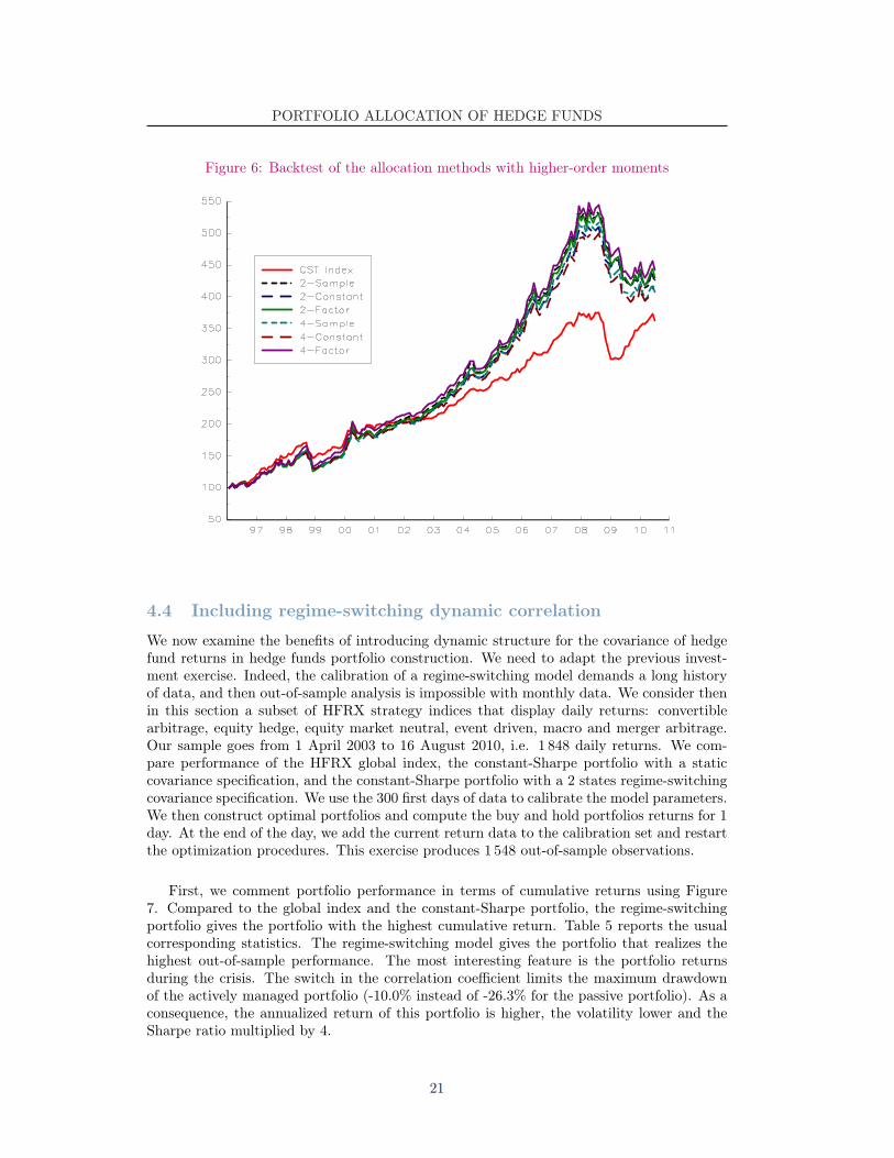
4.3 Including higher-order momentsWe reproduce in this section the same investment exercise, but with the allocation modelsintroduced in Section 3.1. These portfolios are obtained by maximizing a finite dimensionalapproximation of a CARA utility function. They differ on two points: the approximationorder (2 or 4), and the estimators of the higher-order moments (sample moments, constantcorrelation or single factor estimators). We finally get 6 different portfolios. The corre-sponding cumulative returns are plotted in Figure 6.

The risk-adjusted analysis of these six portfolios is presented in Table 4. Panel A reportsthe annualized statistics. We observe that all portfolios have very similar characteristics.However, two main comments can be done. First, we do not significantly increase the skew-ness and decrease the kurtosis of the out-of-sample portfolio when higher-order momentsare included in the objective function. Similarly, the historical drawdown is of the sameorder and occurred during the same period. Second, the sample estimators are always giventhe less performing portfolios. In other words, it is always interesting to add structure tothe estimation of covariance and higher-order moments. Martellini and Ziemann (2010) re-port similar results. Panel B confirms these findings. The Sharpe performance decreases ifhigher-order moments are introduced in the analysis without limiting the estimation risk.The only way to recover the initial global index performance is to use the constant corre-lation estimator together with the 4th order expansion. These disappointing results can beexplained by the use of index data. The non-normality on these indices, i.e. average returns,is not as severe as what we observe on single hedge fund returns. It would be interestingto apply these utility expansion approaches to less normal distributed return assets. Themoment component analysis proposed by Jondeau et al. (2010) is also a promising solutionto control the estimation risk related to the higher moments.

19


Table 4: Out-of-sample performance of efficient portfolios with 1-month rebalancing

Model Estimation Ann. Ret Ann. Vol Skew Kurtosis Max DD Start MDD End MDD


Global index 9.3% 7.8% -0.2 5.7 -19.7% Oct-07 Dec-08

2nd order Sample 10.5% 10.1% -0.3 5.3 -23.3% Feb-08 Jan-10

2nd order Constant 10.6% 9.6% -0.2 4.7 -19.0% Feb-08 Jul-09

2nd order Factor 10.6% 9.8% -0.4 5.5 -21.7% Feb-08 Jul-09

4th order Sample 10.2% 10.0% -0.5 5.0 -24.1% Feb-08 Jan-10

4th order Constant 10.1% 9.4% -0.4 4.4 -22.1% Feb-08 Jul-09

4th order Factor 10.8% 10.1% -0.4 5.2 -21.6% Feb-08 Jul-09

Model Estimation SR TE IR Alpha DD 1M DD 6M DD 1Y


Global index 0.72 -7.5% -19.5% -19.1%

2nd order Sample 0.67 5.7% 0.19 1.1% -10.6% -15.5% -21.4%

2nd order Constant 0.71 5.3% 0.21 1.1% -9.1% -14.4% -17.4%

2nd order Factor 0.70 5.4% 0.22 1.2% -11.1% -15.0% -20.6%

4th order Sample 0.64 5.6% 0.14 0.8% -10.5% -16.3% -22.2%

4th order Constant 0.67 5.2% 0.14 0.7% -9.1% -15.2% -20.6%

4th order Factor 0.70 5.6% 0.24 1.4% -11.2% -15.1% -20.4%

20


Figure 6: Backtest of the allocation methods with higher-order moments

4.4 Including regime-switching dynamic correlation

We now examine the benefits of introducing dynamic structure for the covariance of hedgefund returns in hedge funds portfolio construction. We need to adapt the previous invest-ment exercise. Indeed, the calibration of a regime-switching model demands a long historyof data, and then out-of-sample analysis is impossible with monthly data. We consider thenin this section a subset of HFRX strategy indices that display daily returns: convertiblearbitrage, equity hedge, equity market neutral, event driven, macro and merger arbitrage.Our sample goes from 1 April 2003 to 16 August 2010, i.e. 1 848 daily returns. We com-pare performance of the HFRX global index, the constant-Sharpe portfolio with a staticcovariance specification, and the constant-Sharpe portfolio with a 2 states regime-switchingcovariance specification. We use the 300 first days of data to calibrate the model parameters.We then construct optimal portfolios and compute the buy and hold portfolios returns for 1day. At the end of the day, we add the current return data to the calibration set and restartthe optimization procedures. This exercise produces 1 548 out-of-sample observations.

First, we comment portfolio performance in terms of cumulative returns using Figure7. Compared to the global index and the constant-Sharpe portfolio, the regime-switchingportfolio gives the portfolio with the highest cumulative return. Table 5 reports the usualcorresponding statistics. The regime-switching model gives the portfolio that realizes thehighest out-of-sample performance. The most interesting feature is the portfolio returnsduring the crisis. The switch in the correlation coefficient limits the maximum drawdownof the actively managed portfolio (-10.0% instead of -26.3% for the passive portfolio). As aconsequence, the annualized return of this portfolio is higher, the volatility lower and theSharpe ratio multiplied by 4.

21


Figure 7: Backtest of the allocation methods with HFR Hedge Funds sub-indexes

Table 5: Out-of-sample performance of efficient portfolios with 1-day rebalancing

Model Ann. Ret Ann. Vol Skew Kurtosis Max DD Start MDD End MDD


Global index 0.7% 4.4% -1.2 7.9 -26.3% Jul-07 Dec-08

Equal-weighted 0.6% 3.7% -1.7 11.2 -23.2% Jul-07 Dec-08

Constant-Sharpe -0.5% 3.3% -1.9 16.1 -24.5% Jul-07 Dec-08

regime-switching 2.9% 2.5% -0.8 4.4 -10.0% Jul-07 Nov-08

Model SR TE IR Alpha DD 1M DD 6M DD 1Y


Global index -12.3% -22.9% -23.4%

Equal-weighted 1.6% -0.1 -0.61% -12.1% -20.9% -20.1%

Constant-Sharpe 2.9% -0.4 -2.13% -13.2% -21.3% -21.8%

regime-switching 0.02 3.4% 0.6 0.80% -6.7% -5.6% -7.9%

22


Finally, we briefly discuss the average structure of hedge fund portfolios constructed withthe static and dynamic models. The weights of the assets in the regime-switching portfoliomove faster than the ones obtained in the static case. We note that four strategies, mergerarbitrage, macro, equity market neutral and convertible arbitrage have the highest weightsin the average structure of the regime-switching portfolio. One of the main interestingcharacteristics of the model is to cut the convertible arbitrage exposure during the last crisisand increase it at the beginning of 2009.

In summary, we have found that modeling time-varying covariance of hedge fund returnsimproves our ability to optimize hedge fund portfolio risk. This is reflected in the reducedrisk of the portfolios constructed with the dynamic covariance models relative to the risk ofthe portfolios constructed with the other models.

4.5 Including stress scenarios

Stress scenarios reflect the possibility of extreme drawdowns linked to some rare events.Table 6 gives a canonical example of stress scenarios definition.

Table 6: An example of stress scenarios

Intensity CA SB EM EMN ED FI GM LS CTA MS10% −15% 0 0 0 0 0 0 0 0 010% 0 −15% 0 0 0 0 0 0 0 010% 0 0 −15% 0 0 0 0 0 0 010% 0 0 0 −15% 0 0 0 0 0 010% 0 0 0 0 −15% 0 0 0 0 010% 0 0 0 0 0 −15% 0 0 0 010% 0 0 0 0 0 0 −15% 0 0 010% 0 0 0 0 0 0 0 −15% 0 010% 0 0 0 0 0 0 0 0 −15% 010% 0 0 0 0 0 0 0 0 0 −15%

The possibility of individual drawdowns introduces idiosyncratic risks to the probabilitymeasure, which favor portfolio diversification. As the stress scenarios are the same forall components of the index, the risk level of low volatility components is increased moreproportionally. In other words, less faith is given to low volatility assets. As a result, theallocation procedure leads naturally to better diversified and more homogeneous portfolios,without imposing any diversification constraint. This is confirmed by the following historicalsimulations.

The stress scenarios given in Table 6 illustrate how they can favor diversification. Weonly consider in this example individual drawdowns of the same magnitude, with equalintensities. A deeper study of hedge fund strategies types could lead to more sophisticatedfeatures, such as different magnitudes, intensities, or joined stress scenarios involving someor all of the hedge fund strategies types. Such a study could be based on both quantitativeand qualitative properties of those strategies, for example their risk profiles or their typicalexposure to main asset classes. Furthermore, such fundamental studies on hedge funds orhedge fund classes could highlight hidden risks that a fund of funds manager would bereluctant to take. The stress scenario approach brings an adapted formalization of thoseviews, introducing those expectations into the allocation procedure. Therefore, it can be away to reduce exposure to hedge funds that are considered hazardous by the manager.

23


Figure 8: Backtest of the Stress Scenarios approach

Figure 9: Comparison of average Lorenz curve with and without stress

24


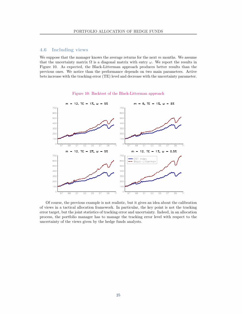
4.6 Including viewsWe suppose that the manager knows the average returns for the next m months. We assumethat the uncertainty matrix Ω is a diagonal matrix with entry ω. We report the results inFigure 10. As expected, the Black-Litterman approach produces better results than theprevious ones. We notice than the performance depends on two main parameters. Activebets increase with the tracking-error (TE) level and decrease with the uncertainty parameter.

Figure 10: Backtest of the Black-Litterman approach

Of course, the previous example is not realistic, but it gives an idea about the calibrationof views in a tactical allocation framework. In particular, the key point is not the trackingerror target, but the joint statistics of tracking error and uncertainty. Indeed, in an allocationprocess, the portfolio manager has to manage the tracking error level with respect to theuncertainty of the views given by the hedge funds analysts.

25


5 ConclusionsTo evaluate the impact of non-normal distribution and time-varying parameters, we illustrateour analysis using an actively managed fund of hedge funds invested in hedge fund indicesfrom the CSFB/Tremont and HFR databases. Our main findings are summarized in thefive following points. First, the application of mean-variance and extension models does notresult in performing portfolios of hedge funds. In terms of risk-adjusted returns, all suchportfolios underperformed the CSFB/Tremont global index portfolio. In other words, activemanagement destroyed value as compared to a static investment in the same underlyings.Second, the inclusion of higher-order moments at the objective function level does not solvethis problem. If the model takes into account more hedge fund returns characteristics, theloss in terms of estimation error is too high. This result persists even when some robustnesstechniques are used at the estimation level. Third, regime-switching dynamic correlationmodels are able to capture changes in correlation between hedge fund strategies and resultin better performing hedge fund portfolios with better diversification. This gives someintuition about the failings of classic models, and implies that the correlation dynamicsbetween hedge fund returns are the main feature allocation models must integrate. Fourth,considering stress scenarios in the allocation process also increases the diversification level ofefficient portfolios. Fifth, views considered in a Black-Litterman framework result in optimalactive portfolios that outperform a static allocation.

26


Appendix

A Mathematical aspects of allocation models

A.1 Shrinkage methodsWe remind that the shrinkage estimator is:

Σα? = α?Φ + (1− α?) Σ

with:α? = max

(0, min

(1T

π − %

γ, 1

))

If Φ is the covariance matrix with a constant correlation10 ρ, we obtain (Ledoit and Wolf,2004):

πi,j =1T

n∑t=1

((xi,t − xi) (xj,t − xj)− Σi,j

)2

ϑi,j =1T

n∑t=1

((xi,t − xi)

2 − Σi,j

)((xi,t − xi) (xj,t − xj)− Σi,j

)

π =n∑

i=1

n∑

j=1

πi,j

% =n∑

i=1

πi,i +n∑

i=1

∑

j 6=i

ρ

2

(√Σj,j

Σi,i

ϑi,j +

√Σi,i

Σj,j

ϑj,i

)

γ =n∑

i=1

n∑

j=1

(Φi,j − Σi,j

)2

In the more general case where Φ is the covariance matrix of the one-factor model, theexpressions of π and γ are the same and % becomes:

% =n∑

i=1

n∑

j=1

%i,j

with %i,i = πi,j and:

%i,j =1T

n∑t=1

%i,j,t

%i,j,t =(Σj,0Σ0,0 (xi,t − xi) + Σi,0Σ0,0 (xj,t − xj)− Σi,0Σj,0

(ft − f

))×(xi,t − xi) (xj,t − xj)

(ft − f

)/Σ2

0,0 − Φi,jΣi,j

In the expression of %i,j,t, we use the augmented matrix Σ corresponding to the empiricalcovariance matrix of (ft, Xt) with the convention that the position of the factor in the matrixis 0. Thus, Σi,0 is the empirical covariance between ft and xi,t, and Σ0,0 is the empiricalvariance of the factor.

10We have Φi,i = Σi,i and Φi,j = ρq

Σi,iΣj,j .

27


A.2 Utility function characteristicsThe two main features of a utility function are the appetite for gain and the risk aversion.The appetite for gain is very natural, and can be translated as “more is better than less”.

A.2.1 Some properties

The appetite for gain is captured by the increasing property of U , i.e. its derivative U ′ ispositive. The other main feature is the investor’s risk aversion, translating the fact that theinvestor would always prefer a fixed wealth to a random wealth with the same expectation.This feature corresponds to the concavity of the function U with respect to terminal wealth.Therefore, for a fixed level of risk, the investor would try to maximize his average return,and controversy, for a fixed level of return the investor would try to minimize his risks. Onthe contrary, a convex utility function (with U ′′ > 0) would imply that the investor is riskseeking and prefers to maximize his risk for a fixed average return.

The qualitative properties of utility functions are now stated, and we can study thequantitative properties of these functions. In particular, there is a clear dilemma betweenthe appetite for high returns and the risk aversion. Indeed, if we consider only one risky assetand a riskless asset, and if this asset has a known positive expected return, then the moneyinvested in the risky asset may range from 0 to +∞ depending of the shape of the utilityfunction. But fortunately, that behavior can be synthesized in a risk aversion coefficient Agiven by −U ′′ (x) /U ′ (x) (or −U ′′ (x) / (xU ′ (x)) when relative wealth is considered. Thiscoefficient may depend of the level of wealth. Two particular cases are interesting: theconstant absolute risk aversion (CARA) or the constant relative risk aversion (CRRA).In the CARA case, with stable market conditions, the optimal investment strategy is tokeep a fixed absolute amount of risk (i.e. a fixed amount of money invested in the riskyasset). Meanwhile, with a CRRA utility, the optimal strategy keeps a fixed proportion ofthe investor’s wealth invested in the risky asset. Therefore, those two fundamental examplesdiffer on the absolute or relative reference to risks.

A.2.2 Fundamental examples

The CARA utility can be shown to be of the form:

U (x) = 1− exp(−x

γ

)

Where the parameter γ is homogeneous to some wealth, and is therefore referred to as thewealth at risk of the utility function. The absolute risk aversion coefficient is equal to 1/γ.Thus, the risk aversion parameter increases naturally as the target wealth at risk decreases.In the case of a single risky asset, it can be shown that the amount w invested in that riskyasset is equal to:

w = γµ− r

σ2

In other words, the volatility of the optimal investment strategy is equal to:

σ (w) = w × σ = γ × sh

where sh is the Sharpe ratio of the risky asset. As the Sharpe ratio of a good risky asset canbe in general estimated around 50%, the parameter γ actually deserves its name of wealthat risk, as it is of the same order of magnitude as the volatility of the optimal portfolio forthis utility function.

28


Meanwhile, the CRRA utility can be written as:

U (x) =xφ

φ

with φ < 1 (in order to ensure a risk adverse behavior). Therefore the relative risk aversioncoefficient is given by:

A = − U ′′ (x)xU ′ (x)

= 1− φ

and the volatility of the optimal allocation is given by:

σ (w) =1

1− φ

µ− r

σ=

sh1− φ

Therefore, the volatility of the optimal allocation has the order of magnitude of the productof the Sharpe ratio of the risky asset and a factor 1/ (1− φ) which represents the risktolerance. Hence, given the value of the Sharpe ratio of the allocation, the risk aversioncoefficient A = 1 − φ may be calibrated to set the volatility of the optimal portfolio at agiven value.

A.3 Computation of the Omega ratio with the Cornish-Fisher ex-pansion

The Cornish Fisher approximation can be described as follows. To obtain a random variableZ with an average µ, a standard deviation σ, a skewness s and an excess Kurtosis κ, it issufficient to consider a polynomial of a standard Gaussian random variable X, that is:

Z = P (X) = µ + σ

(X +

(X2 − 1

) s

6+

(X3 − 3X

) κ

24− (

2X3 − 5X) s2

36

)

as long as the following condition is satisfied:

s2

9− 4

(κ

8− s2

6

)(1− κ

8+

5s2

36

)≤ 0

Therefore, to calculate the Omega ratio:

Ω(H) =E

[(Z −H)+

]

E[(H − Z)+

] =E

[(Z −H)+

]

H − µ + E[(Z −H)+

]

we just have to calculate the expectation of a the positive part of a gaussian polynomial.Let P (x) the function defined by:

P (x) = µ + σ

(x +

(x2 − 1

) s

6+

(x3 − 3x

) κ

24− (

2x3 − 5x) s2

36

)

A simple calculus gives:

P (x) = µ− σs

6+ σ

((1− κ

8+

5s2

36

)x +

s

6x2 +

(κ

24− s2

18

)x3

)

= Q (x)

29


Using this result, the formula of the expected return above H when the distribution is givenby the Cornish Fisher expansion is:

E((Z −H)+

)=

∫ ∞

P−1(H)

1√2π

P (x) e−x22 dx

=∫ ∞

P−1(H)

1√2π

Q (x) e−x22 dx

=(µ− σ

s

6

)A0 (H) + σ

(1− κ

8+

5s2

36

)A1 (H) +

σs

6A2 (H) + σ

(κ

24− s2

18

)A3 (H)

where the coefficient A0, A1, A2 and A3 are given by the following expressions :

A0 (H) =∫ ∞

P−1(H)

1√2π

e−x22 dx

= 1− Φ(P−1 (H)

)

A1 (H) =∫ ∞

P−1(H)

1√2π

xe−x22 dx

=[− 1√

2πe−

x22

]∞

P−1(H)

=1√2π

e−(P−1(H))2

2

A2 (H) =∫ ∞

P−1(H)

1√2π

x2e−x22 dx

=[− 1√

2πxe−

x22

]∞

P−1(H)

+∫ ∞

P−1(H)

1√2π

e−x22 dx

=1√2π

P−1 (H) e−(P−1(H))2

2 + 1− Φ(P−1 (H)

)

A3 (H) =∫ ∞

P−1(H)

1√2π

x3e−x22 dx

=[− 1√

2πx2e−

x22

]∞

P−1(H)

+∫ ∞

P−1(H)

2x√2π

e−x22 dx

=1√2π

(P−1 (H)

)2e−

(P−1(H))2

2 +2√2π

e−(P−1(H))2

2

Anyway, we must make sure that the Cornish Fisher expansion is well defined. This randomvariable defined by this expansion must be an increasing function of the underlying gaussianvariable. This is insured by the following condition:

s2

9− 4

(κ

8− s2

6

)(1− κ

8+

5s2

36

)≤ 0

By denoting κ = κ8 and s = s2

9 , we obtain:

s− 4(

κ− 3s

2

)(1− κ +

5s

4

)≤ 0

30


As we only look for a sufficient condition, we first consider the case where s = 0. In thatcase, the condition reduces to −4κ (1− κ) ≤ 0. Thus the condition is satisfied for 0 ≤ κ ≤ 1.If we suppose that it is fulfilled, we have the condition:

s− 4(

κ− 3s

2

)(1− κ +

5s

4

)= s− 4

(κ− κ2 +

5sκ

4− 3s

2+

3sκ

2− 15s2

8

)

= 4(κ2 − κ

)+ (7− 11κ) s2 +

15s2

2≤ 0

Resolving this polynomial inequation, we finally find the sufficient condition:

s ≤11κ− 7 +

√(11κ− 7)2 − 120 (κ2 − κ)

15

A.4 Higher-order momentsThe second moment tensor M2 corresponds to the usual variance-covariance matrix:

M2 = E[(R− E [R]) (R− E [R])>

]

The representations of M3 and M4 use a column-wise approach that gives the followingexpression of the coskewness of assets i, j and k:

si,j,k = E [(Ri − µi) (Rj − µj) (Rk − µk)]

and the cokurtosis of assets i, j, k and l:

κi,j,k,l = E [(Ri − µi) (Rj − µj) (Rk − µk) (Rl − µl)]

where Ri denotes the return of asset i and µi its expected return. To illustrate this column-wise representation, we give the higher-order moment tensors M3 and M4 for n = 3 assets:

M3 =[

S1 | S2 | S3

]

M4 =[

K1,1 K1,2 K1,3 | K2,1 K2,2 K2,3 | K3,1 K3,2 K3,3

]

where:

Sp =

sp,1,1 sp,1,2 sp,1,3

sp,2,1 sp,2,2 sp,2,3

sp,3,1 sp,3,2 sp,3,3

, Kp,q =

κp,q,1,1 κp,q,1,2 κp,q,1,3

κp,q,2,1 κp,q,2,2 κp,q,2,3

κp,q,3,1 κp,q,3,2 κp,q,3,3

are n× n matrices. Using the Kronecker product, the higher-order moment tensors can berepresented as follows:

M3 = E[(R− E [R]) (R− E [R])> ⊗ (R− E [R])>

]

M4 = E[(R− E [R]) (R− E [R])> ⊗ (R− E [R])> ⊗ (R− E [R])>

]

Thus, the expressions of the portfolio centered moments are polynomial functions in then× 1 vector of the underlying asset weights w:

µ(2) = w>M2w

µ(3) = w>M3 (w ⊗ w)µ(4) = w>M4 (w ⊗ w ⊗ w)

31


Assuming that the wealth W is equal to the final portfolio value and with an initial wealthequal to one, we can write the expected utility as a function of the portfolio weights:

E [U (W )] ' U(w>µ

)+

12U (2)

(w>µ

)w>M2w +

16U (3)

(w>µ

)w>M3 (w ⊗ w) +

124

U (4)(w>µ

)w>M4 (w ⊗ w ⊗ w)

The investor’s optimization problem is then to maximize this approximated expected utilitywith respect to the w.

A.5 Stress scenarios properties

A.5.1 Average time between two stress scenarios

The probability of occurrence of a stress scenario is defined through the concept of intensity,derived from the theory of Poisson processes. A given level of intensity λ means that thestress scenario has a probability λ∆t of occurrence during any small time interval ∆t. Thus,the parameter λ can be interpreted as the yearly probability of occurrence of the scenario.Therefore, a scenario is observed more frequently if its intensity λ is high. The frequency ofstress scenario observation is therefore proportional to the intensity. From this definition,we can easily calculate the average time between two observations of the same scenario. Ifwe denote the last scenario observation date as t = 0, and the next occurrence date of thesame scenario as τ , the probability that the same scenario occurs after a given time t is bedenoted as:

P (t) = P τ > tFor small dt, it satisfies the following equation:

P τ > t − P τ > t + dt = P t + dt > τ > t= P t + dt > τ | τ > t · P τ > t= λP τ > t dt

Therefore, we get the differential equation:

dP (t) = −λP (t) dt

Using the fact that P (0) = 1, we obtain:

P (t) = e−λt

Then, integrating the probability distribution of t gives us the average time between twostress scenarios:

E [τ ] =∫ +∞

0

−tdP

dtdt

=∫ +∞

0

λte−λt dt

=1λ

The average time between two stress scenarios is indeed the inverse of its intensity.

32


A.5.2 Stressing the probability distribution

Stress scenarios can be added when using either parametric or empirical probability distri-butions. Any criterion relying on an expectation of a function of the portfolio returns isbased on a computation of:

EP [f (rwt )]

where rwt is the random return of the portfolio w over some period t, characterized by

its distribution P. We introduce K stress scenarios, which would lead to a performancerwsk

for strategy w and scenario sk. The probability of each of those scenarios to occur isproportional to the length of the backtesting period. Typically, a stress scenario has a 10%probability to happen each year. We denote by λk the yearly probability of appearanceof the k-th scenario, i.e. the stress intensity. The average number of occurrence of eachscenario is then λkt, while the probabilities of other events sum to 1. Thus, the new formulato compute the stress expectation is given by:

E [f (rwt )| s1, . . . , sK ] =

1

1 +∑K

k=1 λkt

(EP [f (rw

t )] +k∑

k=1

λktf(rwsk

))

A.5.3 Case of the empirical distributions

With the empirical distribution, we include some hypothetical scenarios into the set of his-torical returns. The difference between those fictitious stress scenarios and actual historicalobservations is their probabilities. In particular, without stress scenarios, backtesting overn months an allocation w leads to an historical monthly performance rw

t , with t rangingfrom 1 to n. In that case, the standard empirical distribution is obtained by consideringthat each return occurs with an equal probability 1

n . Thus, the expected utility given bythis allocation is:

U (w) =1∑e αe

×(∑

e

αe × U (e)

)

where e is the event and αe is the weight of the event. We obtain, with stress scenarios:

U (w) =1

n + n∆t

∑Kk=1 λk

(n∑

t=1

U (1 + rwt ) + n∆t

K∑

k=1

λkU(1 + rw

sk

))

=1

1 + ∆t

∑Kk=1 λk

(n−1

n∑t=1

U (1 + rwt ) +

K∑

k=1

∆tλkU(1 + rw

sk

))

In general, the expectation of any function of the assets returns can be written as:

E [f (r)| s1, . . . , sK ] =1

1 + ∆t

∑Kk=1 λk

(n−1

n∑t=1

f (rt) +K∑

k=1

∆tλkf (rsk)

)

A.6 Black-Litterman approachWe assume that the vector µ of expected returns is unknown and we have:

µ ∼ N (π, Γ)

The views of the fund manager are given by:

Pµ = Q + ε

33


where P is a k×n matrix Q is a k× 1 vector and ε ∼ N (0,Ω) is a gaussian random vector.Let µcond the conditional expected return defined by the following optimization program:

µcond = arg min (µ− π)> Γ−1 (µ− π)u.c. Pµ = Q + ε

We may show the solution is:

µcond = E [µ | Pµ = Q + ε]

=(Γ−1 + P>Ω−1P

)−1 (Γ−1π + P>Ω−1Q

)

After some computations, we finally obtain11:

µcond = π + ΓP>(PΓP> + Ω

)−1(Q− Pπ) (4)

From a practical point of view, the following steps to implement the Black-Litterman modelare:

1. We compute the empirical covariance matrix Σ. Given the portfolio allocation w0, wededuce the expected returns π as the solution of the inverse mean-variance problem:

π =2λ

Σ−1w

2. We define the views of the fund manager by specifying the matrices P , Q, Γand Ω.We then compute the conditional expected returns µcond given by equation (4).

3. We then solve the traditional tracking error problem:

max w>µcond u.c. (w − w0)>Σ (w − w0) ≤ σ2

TE

with σTE the maximum level of the tracking error volatility.

11Using the following result on matrix inversion:“A + XBX>

”−1= A−1 −A−1X

“B−1 + X>A−1X

”−1X>A−1

we obtain: “Γ−1 + P>Ω−1P

”−1= Γ− ΓP>

“Ω + PΓP>

”−1PΓ

We deduce that:

µcond =

„Γ− ΓP>

“Ω + PΓP>

”−1PΓ

«“Γ−1π + P>Ω−1Q

”

= π − ΓP>“Ω + PΓP>

”−1 “Pπ + PΓP>Ω−1Q

”+ ΓP>Ω−1Q

= π − ΓP>“Ω + PΓP>

”−1Pπ + ΓP>

„Ω−1 −

“Ω + PΓP>

”−1PΓP>Ω−1

«Q

= π − ΓP>“Ω + PΓP>

”−1Pπ + ΓP>

“Ω + PΓP>

”−1Q

34


References[1] Ackermann C., McEnally R. and Ravenscraft D. (1999), The Performance of

Hedge Funds: Risk, Return, and Incentives, Journal of Finance, 54, pp. 833-874.

[2] Adam A., HoukariM. and Laurent J.P. (2008), Spectral Risk Measures and PortfolioSelection, Journal of Banking and Finance, 32, pp. 1870-1882.

[3] Agarwal V., Bakshi G. and Huij J. (2009), Do Higher-Moment Equity Risks ExplainHedge Fund Returns? Robert H. Smith School Research Paper, 06-066.

[4] Agarwal V. andNaik N. (2004), Risks and Portfolio Decisions Involving Hedge Funds,Review of Financial Studies, 17, pp. 63-98.

[5] Alexander C. and Dimitriu A. (2004), The Art of Investing in Hedge Funds: FundSelection and Optimal Allocation, ICMA Centre Working Papers.

[6] Amenc N. and Martellini L. (2002), Portfolio Optimization and Hedge Fund StyleAllocation Decisions, Journal of Alternative Investments, 5, pp. 7-20.

[7] Amin G. and Kat H. (2003), Stocks, Bonds, and Hedge Funds, Journal of PortfolioManagement, 29, pp. 113-120.

[8] Ang A. and Chen J. (2002), Asymmetric Correlations of Equity Portfolios, Journal ofFinancial Economics, 63, pp. 443-494.

[9] Bares P., Gibson R. and Gyger S. (2002), Hedge Fund Allocation with SurvivalUncertainty and Investment Constraints, Working Paper.

[10] Berkowitz J. (2000), A Coherent Framework for Stress Testing, Journal of Risk, 2,pp. 1-11.

[11] Billio M., Getmanski M. and Pelizon S. (2010), Crises and Hedge Funds Risk,Working Paper.

[12] Bollerslev T. (1990), Modelling the Coherence in Short-run Nominal ExchangeRates: A Multivariate Generalized ARCH Model, Review of Economics and Statistics,72, pp. 498-505.

[13] Brooks C. and Kat (2002), The Statistical Properties of Hedge Fund Index Returnsand their Implications for Investors, Journal of Alternative Investments, 5, pp. 26-44.

[14] Brown S., Goetzmann W. and Ibbotson R. (1999), Offshore Hedge Funds: Survivaland Performance 1989-1995, Journal of Business, 72, pp. 91-118.

[15] Buraschi A., Kosowski R. and Trojani F. (2010), When There Is No Place toHide: Correlation Risk and the Cross-Section of Hedge Fund Returns, Imperial College,Working Paper.

[16] Chan N., Getmansky M., Haas S. and Lo A. (2006), Do Hedge Funds IncreaseSystemic Risk?, Federal Reserve Bank of Atlanta Economic Review, Q4, pp. 49-80.

[17] Choueifaty Y. and Coignard Y. (2008), Towards Maximum Diversification, Journalof Portfolio Management, 35, pp. 40-51.

[18] Clarke R., de Silva H. and Thorley S. (2006), Minimum-variance Portfolios in theU.S. Equity Market,Journal of Portfolio Management, 33, pp. 10-24.

35


[19] Cont R. (2001), Empirical Properties of Asset Returns: Stylized Facts and StatisticalIssues, Quantitative Finance, 1, pp. 223-236.

[20] Cvitanic J., Lazrak A.,Martellini L. and Zapatero F. (2003), Optimal Allocationto Hedge Funds: An Empirical Analysis, Quantitative Finance, 3, pp. 1-12.

[21] Darolles S. and Gourieroux C. (2010), Conditionally Fitted Sharpe Performancewith an Application to Hedge Fund Rating, Journal of Banking and Finance, 34, pp.578-593

[22] Darolles S., Gourieroux C. and Jasiak J. (2009), L-Performance with an Appli-cation to Hedge Funds, Journal of Empirical Finance, 16, pp. 671-685

[23] Darolles S. and Mero M. (2010), Hedge Fund Returns and Factor Models: TheFactor Selection Puzzle, Bankers Markets and Investors, forthcoming.

[24] Darolles S. and Vaissie M. (2010), Do Funds of Hedge Funds Really Add Value?,Working paper.

[25] Davies R., Kat H. and Lu S. (2009), Fund of Hedge Funds Portfolio Selection: AMultiple-objective Approach, Journal of Derivatives and Hedge Funds, 15, pp. 91-115.

[26] Eling M. and Schumacher F. (2007), Does the Choice of Performance Measure In-fluence the Evaluation of Hedge Funds?, Journal of Banking and Finance, 31, pp.2632-2647.

[27] Elton E.J. and Gruber M.J. (1973), Estimating the Dependence Structure of SharePrices — Implications for Portfolio Selection, Journal of Finance, 28, pp. 1203-1233.

[28] Engle R. (2002), Dynamic Conditional Correlation, Journal of Business and EconomicStatistics, 20, pp. 339-350.

[29] Favre L. and Galeano J. (2002), Mean-Modified Value-at-Risk Optimization withHedge Funds, Journal of Alternative Investments, 5, pp. 21-25.

[30] Fung W. and Hsieh D. (1997), Empirical Characteristics of Dynamic Trading Strate-gies: The Case of Hedge Funds, Review of Financial Studies, 10, pp. 275-302.

[31] Fung W. and Hsieh D. (1999), A Primer on Hedge Funds, Journal of Empirical Fi-nance, 6, pp. 309-331.

[32] Fung W. and Hsieh D. (2001), The Risk in Hedge Fund Strategies: Theory andEvidence from Trend Followers, Review of Financial Studies, 14, pp. 313-341.

[33] Getmansky M, Lo A. and Makarov I. (2004), An Econometric Model of SerialCorrelation and Illiquidity in Hedge Fund Returns, Journal of Financial Economics,74, pp. 529-610.

[34] Giomouridis D. and Vrontos I. (2007), Hedge Fund Portfolio Construction: A Com-parison of Static and Dynamic Approaches, Journal of Banking and Finance, 31, pp.199-217.

[35] Greyserman A., Jones D. and Strawderman W. (2006), Portfolio Selection usingHierarchical Bayesian Analysis and MCMC Methods, Journal of Banking and Finance,30, pp. 669-678.

36


[36] Hagelin N. and Pramborg B. (2003), Evaluating Gains from Diversifying into HedgeFunds Using Dynamic Investment Strategies, in Schachter, B. (eds), Intelligent HedgeFund Investing, Risk Books, London.

[37] Jondeau E. and Rockinger M., (2006), Optimal Portfolio Allocation Under HigherMoments, European Financial Management, 12, pp. 29-55.

[38] Jondeau E., Jurczenko E. and Rockinger M., (2010), Moment Component Anal-ysis: An Illustration with International Stock Markets, Working paper.

[39] Jurczenko E, Maillet B. and Merlin P. (2005), Hedge Funds Portfolio Selectionwith Higher-order Moments: A Non-parametric Mean-Variance-Skewness-Kurtosis Ef-ficient Frontier, Working paper.

[40] Kat H. (2004), In Search of the Optimal Fund of Hedge Funds, Journal of WealthManagement, 6, pp. 43-51.

[41] Krokhmal P., Uryasev S. and Zrazhevsky G. (2002), Risk Management for HedgeFund Portfolios: A Comparative Analysis of Linear Portfolio Rebalancing Strategies,Journal of Alternative Investments, 5, pp. 10-29.

[42] Ledoit O and Wolf M. (2003), Improved Estimation of the Covariance Matrix ofStock Returns With an Application to Portfolio Selection, Journal of Empirical Fi-nance, 10, pp. 603-621.

[43] Ledoit O. and Wolf M. (2004), Honey, I Shrunk the Sample Covariance Matrix,Journal of Portfolio Management, 30, pp. 110-119.

[44] Liew J. (2003), Hedge Fund Index Investing Examined, Journal of Portfolio Manage-ment, 29, pp. 113-123.

[45] Maillard S., Roncalli T. and Teiletche J. (2010), The Properties of EquallyWeighted Risk Contribution Portfolios, Journal of Portfolio Management, 36, pp. 1-11.

[46] Malkiel B.G. and Saha A. (2005), Hedge Funds: Risk and Return, Financial AnalystsJournal, 61, pp. 80-88.

[47] Martellini L. (2008), Toward the Design of Better Equity Benchmarks, Journal ofPortfolio Management, 34, pp. 1-8.

[48] Martellini L. and Ziemann V. (2010), Improved Estimates of Higher-Order Como-ments and Implications for Portfolio Selection, Review of Financial Studies, 23, pp.1467-1502.

[49] Markowitz H. (1952), Portfolio Selection, Journal of Finance, 7, pp. 77-91.

[50] McFall Lamm R. (2003), Asymmetric Returns and Optimal Hedge Fund Portfolios,Journal of Alternative Investments, 6, pp. 9-21.

[51] Michaud R. (1989), The Markowitz Optimization Enigma: Is Optimized Optimal?,Financial Analysts Journal, 45, pp. 31-42.

[52] Merton R. (1980), On estimating the Expected Return on the Market: An ExploratoryInvestigation, Journal of Financial Economics, 8, pp. 323-361.

37


[53] Morton D., Popova E. and Popova I. (2006), Efficient Fund of Hedge Funds Con-struction Under Downside Risk Measures, Journal of Banking and Finance, 30, pp.503-518.

[54] Pelletier D. (2006), Regime Switching for Dynamic Correlations, Journal of Econo-metrics, 131, pp. 445-473.

[55] Popova I., Morton, D. and Popova E. (2003), Optimal Hedge Fund Allocation withAsymmetric Preferences and Distributions, University of Texas, Working paper.

[56] Rockafellar R., Uryasev S. and Zabarankin M. (2006), Master Funds in PortfolioAnalysis with General Deviation Measures, Journal of Banking and Finance, 30, pp.743-778.

[57] Shadwick W. and Keating C. (2002), A Universal Performance Measure, Journal ofPerformance Measurement, 6, pp. 59-84.

[58] Sharpe W. (1963), A Simplified Model for Portfolio Analysis, Management Science, 8,pp. 277-293.

[59] Sharpe W. (2007), Expected Utility Asset Allocation, Financial Analysts Journal, 63,pp. 18-30.

[60] Terhaar K., Staub R. and Singer B. (2003), Appropriate Policy Allocation forAlternative Investments, Journal of Portfolio Management, 29, pp. 101-111.

[61] Von Neumann J. and Morgenstern O. (1953), Theory of Games and EconomicBehavior, Princeton University Press.

38

PortfolioAllocation ofHedgeFunds - Thierry Roncalli · PortfolioAllocation ... funds portfolio is...

Documents

Transcript of PortfolioAllocation ofHedgeFunds - Thierry Roncalli · PortfolioAllocation ... funds portfolio is...