WP/04/109

Performance of Western Hemisphere Trading Blocs:

A Cost-Corrected Gravity Approach

Enzo Croce, V. Hugo Juan-Ramón, and Feng Zhu

© 2004 International Monetary Fund WP/04/109

IMF Working Paper

IMF Institute

Performance of Western Hemisphere Trading Blocs: A Cost-Corrected Gravity Approach

Prepared by Enzo Croce, V. Hugo Juan-Ramón, and Feng Zhu1

June 2004

Abstract

This Working Paper should not be reported as representing the views of the IMF. The views expressed in this Working Paper are those of the author(s) and do not necessarily represent those of the IMF or IMF policy. Working Papers describe research in progress by the author(s) and are published to elicit comments and to further debate.

We study the performance of the four Western Hemisphere trading blocs during the period 1978–2001. For the North American Free Trade Agreement (NAFTA), trade integration outweighed trade diversion; for MERCOSUR, increased integration and trade diversion wenthand in hand; for the Central American Common Market (CACM) and the Andean Community, the evidence points to trade diversion only. We also find that trade among neighboring countries has increased since the early 1990s. The estimations are based on a nonlinear gravity equation that incorporates the hypothesis that exports create externalities that affect trade costs. This hypothesis might help reconcile the theoretical unitary income elasticity with most empirical findings of a non-unitary income elasticity in studies using the gravity equation. JEL Classification Numbers: F14, F15 Keywords: Trading blocs, externalities, trade integration and trade diversion,

Western Hemisphere Author’s E-Mail Address: ecroce@imf.org; vjuanramon@imf.org; zhufeng@ssc.upenn.edu

1 Mr. Zhu was a summer intern at the IMF Institute during 2003. The authors are grateful to Adolfo Barajas, Mercedes Da Costa, Andrew Feltenstein, and Yongzheng Yang for their very useful comments. Remaining errors are the responsibility of the authors.

- 2 -

Contents Page

I. Introduction....................................................................................................................3 II. Theoretical Motivation...................................................................................................4 III. Empirical Model ............................................................................................................7 IV. Results............................................................................................................................8 V. Conclusions..................................................................................................................18 Appendix I. Data Descriptions.........................................................................................................19 II. The Trade Cost Factor and the Volume of Trade, and the Cost of Bilateral Resistance ....................................................................................................................20 Figures 1. Estimated Coefficients for Economic Mass, Distance, Adjacency, and Shared

Language......................................................................................................................13 2. MERCOSUR: Estimated Gravity Model Coefficients ................................................14 3. NAFTA: Estimated Gravity Model Coefficients.........................................................15 4. CACM: Estimated Gravity Model Coefficients ..........................................................16 5. Andean Community: Estimated Gravity Model Coefficients......................................17 Tables 1. Estimated Coefficients of the Cost-Corrected Gravity Model.....................................12 2. Sample of 64 Economies .............................................................................................19 References................................................................................................................................22

- 3 -

I. INTRODUCTION Since the early 1990s, there has been an upsurge of trading blocs worldwide. The World Trade Organization (WTO) reports a total of 240 regional trade agreements (RTAs) globally, of which 70 percent were “in force” as of July 2000. Because the empirical evidence is not conclusive so far, economists have been divided on the wisdom of such arrangements. Further research on this topic is therefore needed. This paper investigates the performance of the main trading blocs in the Western Hemisphere by estimating a nonlinear gravity equation that incorporates a novel trade cost factor.2 Concretely, we ask the following questions: How might the empirical finding of non-unitary income elasticity be interpreted? Are these trading blocs effective in promoting trade? And do they generate more trade diversion than integration? Economists’ opinions on the welfare effects of trading blocs have varied widely, with some seeing them as beneficial and others arguing the opposite. Ethier (1998, p. 1214) states that “regional integration, far from threatening multilateral liberalism, may in fact be a direct consequence of the success of past multilateralism and an added guarantee for its survival.” Summers (1993) argues that regionalism is beneficial if, among other conditions, it happens among “natural trading partners.” 3 However, the evidence is still inconclusive as to whether trading blocs are welfare improving. Panagariya (1999, p. 485) argues that “trade diversion is not something that can be laughed off” and that the “natural trading partners hypothesis has no analytical basis.” On the empirical side, Yeats (1997) claims to have found “smoking gun” evidence that trade diversion dominates trade creation in MERCOSUR. Krueger (1999) finds that, until 1997, the impact of NAFTA does not appear to have been large relative to the effects of other events, such as Mexico’s reduction of tariffs and nontariff restrictions and its move to a more flexible exchange rate policy. And Soloaga and Winters (1999) argue that all major trading blocs in the Western Hemisphere are irrelevant in promoting trade. 4 2 The four trading blocs in the Western Hemisphere are: The North American Free Trade Agreement (NAFTA); Southern Common Market (MERCOSUR); Central American Common Market (CACM); and the Andean Community.

3 This optimistic viewpoint, together with frustration about the slow pace of multilateral negotiations, has had policy implications. The United States, a supporter of multilateralism, became an active participant in RTAs. In 1985 the United States signed its first bilateral trade agreement with Israel, and since then it has orchestrated several trade agreements, including NAFTA. Furthermore, the United States is expected to participate in the 34-nation Free Trade Area of the Americas (FTAA), the largest trading bloc in history, which is slated to take effect in 2005. 4 Arguably, security, democracy, and upholding the rule of law might be major reasons other than trade behind the formation of blocs.

- 4 -

Most empirical research on trading blocs uses the gravity model,5 which states that the volume of international trade is correlated with the size of the trading countries, the costs of trade, and other country-specific variables. Following Anderson and Van Wincoop (2001), and Coe, Subramanian, Tamirisa, and Bhavnani (CSTB; 2002), we use a nonlinear variant of the gravity model and apply it to a sample of 64 industrial and developing economies (listed in Table 2, Appendix I) for the period 1978–2001. Our results confirm the finding of most empirical research that the income elasticity of trade is larger than zero but less than one. We will argue that this can be reconciled with the standard gravity model by assuming that exports generate net negative externalities that increase the trade cost factor and slow down the rate of trade expansion. We also find that geographical distance and a shared language have become somewhat less relevant over time in explaining trade among countries, and that trade among neighboring countries increased in the early 1990s. This last finding, which is seemingly at odds with the finding that “distance” has become somewhat less relevant, might reflect the global surge in RTAs that occurred about that time. As for the performance of the main trading blocs in the Western Hemisphere, we find that for NAFTA, trade integration outweighed trade diversion; for MERCOSUR, trade integration and trade diversion went hand in hand; and for CACM and the Andean Community, the evidence points basically to trade diversion.6

II. THEORETICAL MOTIVATION We extend the basic gravity model proposed in Anderson and Van Wincoop (2001) by assuming that exports generate both positive and negative externalities, which in turn affect trade. This extension might help explain the non-unitary income elasticity found in most empirical estimations of the gravity equation. This model’s key variables include the economic size of the trading countries or regions (as measured by GDP), a trade cost factor, and country-specific effects. In particular, the trade cost factor causes a discrepancy between the exporter’s and the importer’s prices:

ij i ijp p t= × , (1)

where 1ijt ≥ is the trade cost factor, which makes pij (the price of a good produced in country i to consumers in country j, including trade costs) higher than pi (the exporter’s supply price, 5 For a review of recent theoretical treatments, see Frankel (1997) and Anderson and Van Wincoop (2001).

6 “Trade integration” reflects intra-bloc trade resulting from the regional trading agreement. However, not necessarily does it reflect “trade creation.” This is because more intra-bloc trade could instead reflect a shift from low-cost producers in the rest of the world to higher cost producers in the regional trading bloc.

- 5 -

net of trade costs). In a maximizing, general equilibrium setup under certain assumptions—that each region specializes in producing a fixed supply of only one good; that trade costs create a wedge between the exporter’s and the importer’s price; and that consumers in different countries have identical, homothetic preferences, approximated by a constant-elasticity-of-substitution utility function—Anderson and Van Wincoop derive the following gravity equation:

1

i j ijij w

i j

GDP GDP tX

GDP P P

σ− ×

= × , (2)

where Xij is consumption of country i good by country j consumers (that is, exports from country i to country j); GDPw is world GDP; 1σ > is a parameter in the utility function (the elasticity of substitution between any two goods); and Pi and Pj are, in Anderson and Van Wincoop’s terminology, “multilateral resistance” variables, because they depend on all bilateral resistances tij, including those not directly involving i. The gravity equation (2) says that trade between countries i and j is determined by the product of two components: the relative economic mass, and the relative trade resistance. The first is measured as the product of both countries’ GDP divided by world GDP, and the second as the bilateral trade resistance between countries i and j divided by the multilateral trade resistance (that is, the trade resistance that both countries face from all their trading partners). An important feature of the traditional gravity model as represented by equation (2) is that, the elasticity of exports with respect to income (that is, relative economic mass) is unitary. This, however, has been at odds with most empirical studies, which estimate an income elasticity between zero and one. The model that we apply in this paper is an extension of equation (2), derived by incorporating the hypothesis that trade might create either positive or negative externalities that affect the trade cost factor. Thus distance, although important in determining trade patterns, would not be the only variable associated with the trade cost factor, as is usually the case. A variety of arguments can be invoked to support the hypothesis that the volume of trade reduces the trade cost factor. Roberts and Tybout (1997) and Bernard and Wagner (1998) found that sunk costs play an important role in firms’ supply decisions and that prior export experience increases the probability that a firm will export more. Anderson (1999) stresses the role of group ties (or networks): more trade leads to more connections, which help decrease the average cost of trade. Also, in the presence of external pecuniary and technical economies, more trade might reduce trade costs. Thus extending these results to the country level has an intuitive appeal. Alternatively, infrastructure and institutional restrictions (bottlenecks), intrusive regulations, technical diseconomies, trade financing constraints, local bias, and special interest politics (vested interest groups) suggest that more trade leads to more friction, which in turn slows down further trade expansion.

- 6 -

Therefore we postulate that the trade cost factor between countries i and j increases with distance and may either increase or decrease with trade:

( )

( )

/ 1

/ 1ij

ijij

dt

X

β σ

η σ

−

− −= , (3)

where dij is the distance between countries i and j; Xij stands for consumption of country i good by country j consumers (that is, exports from country i to country j); β < 0; –1 < η < 1; and 1 – σ < 0. Whereas β and η are key parameters, (1 – σ) is a scale factor for algebraic convenience and cancels out once we substitute the trade cost factor in equation (2). Thus the greater the distance between two countries, the higher will be the trade cost factor between those countries compared with other pairs of countries that are closer geographically. And more exports from country i to country j will either reduce tij, if positive externalities dominate (0 < η < 1); or increase it, if negative externalities dominate (–1 < η < 0); or have no effect, if positive and negative externalities offset each other (η = 0). Equations (2) and (3) imply that

1111

11i jij ijw

i j

GDP GDPX d

P PGDP

σβηηη

−−−

− ×

= × . (4)

Equation (4) says that countries i and j will trade more, the shorter is the distance between them, the higher their multilateral resistance (that is, i’s resistance to trade with all countries and j’s resistance to trade with all countries), and the greater their economic mass relative to the world economic mass. The magnitude of this last effect is given by the elasticity of trade with respect to this relative economic mass, 1/(1 – η). This elasticity could be either larger than one if trade generates net positive externalities, smaller than one if trade generates net negative externalities, or equal to one if the positive and negative externalities offset each other.7

7 Using our specification of the trade cost factor, equation (4) and the cost of bilateral resistance are derived in Appendix II.

- 7 -

III. EMPIRICAL MODEL

On the basis of equation (4) and including the relevant country-specific variables, we propose the following nonlinear empirical model:8

( ) 1, 2, ijt tijt it jt it jt ij ijtExport GDP GDP POP POP d e

α µδ δ βγ ε= × × × × × × + (5)

with ij5ij4ij3jb2ib1jiij AλLλΒλPTIλPTEλκθµ ++++++= ,

where Exportijt stands for exports from country i to country j during period t; POP stands for population; dij measures distance between countries i and j; θi is a fixed effect for country i; кj is a fixed effect for country j; ibΡΤE and jbΡΤΙ are trading bloc-specific dummy variables capturing each bloc’s propensity to export and import, respectively;9 Bij is another trading bloc-specific dummy variable that equals one when both countries are members of the same one of the four blocs in the Western Hemisphere (this measures the overall trade integration within a particular bloc); Lij is a dummy variable equal to one if countries i and j share a common language (this variable captures the degree of trade friction due to cultural and linguistic differences); Aij is a dummy variable equal to one if countries i and j share a common border; and εij is a “well-behaved” error term. The two variables measuring the bloc’s propensity to export and import (similar to the propensities to export and import for a given country) capture each bloc’s trade diversion effects, as in Soloaga and Winters (1999). One can interpret a decrease in a bloc’s propensity to export or import concomitant with the formation of a trade bloc as a possible trade diversion (or import substitution) effect related to that trade bloc.10 8 As indicated by CSTB, there are three main reasons for using a nonlinear specification of the gravity equation: (1) it allows one to use zero entries in the trade data; (2) when GDP goes to zero, trade should be zero, which is only captured by a nonlinear specification; and (3) the nonlinear regression has a better fit than the linear one. We think that an additional reason is that when running alternative regression specifications (not reported here) we found that error terms behave better under a nonlinear than they do under a linear specification. 9 Let the subscript b represent the four blocs in the Western Hemisphere: 1, ... , 4. If country i (exporter) belongs to bloc 1, but country j (importer) does not belong to bloc 1, then PTEi1 = 1. If j (importer) belongs to bloc 1, but i (exporter) does not belong to bloc 1, then PTIj1 = 1. Otherwise, if i and j either both belong to the same bloc or do not belong to any bloc, then PTEib and PTIjb are both zero.

10 Although we focus on the four trading blocs in the Western Hemisphere, in our estimations other large trading blocs outside the region are also taken into account. However, when we do this, results do not change significantly.

- 8 -

Our nonlinear version of the gravity equation is used to estimate the time path of the key coefficients by running a cross-section regression for each year in our sample.11 This might be a more efficient way to assess trading blocs’ performance over time than alternative strategies proposed in the literature. For example, Dell’Ariccia (1999) uses pooled (or single-year) data to test the performance of a specific trading bloc. However, this approach could yield misleading results because dummy variables (that capture ex post effects) are affected by many temporary factors in a single year. Krueger (1999) estimates recursively the time path of the trading bloc dummies while maintaining the other coefficients in the model constant. But this method would give unbiased estimations only if the estimated coefficients were drawn from the same distribution, which might not be the case.

IV. RESULTS

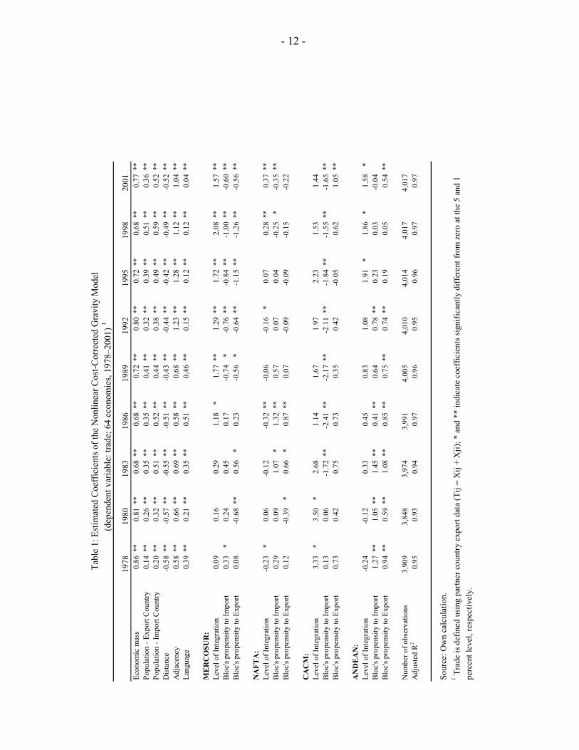
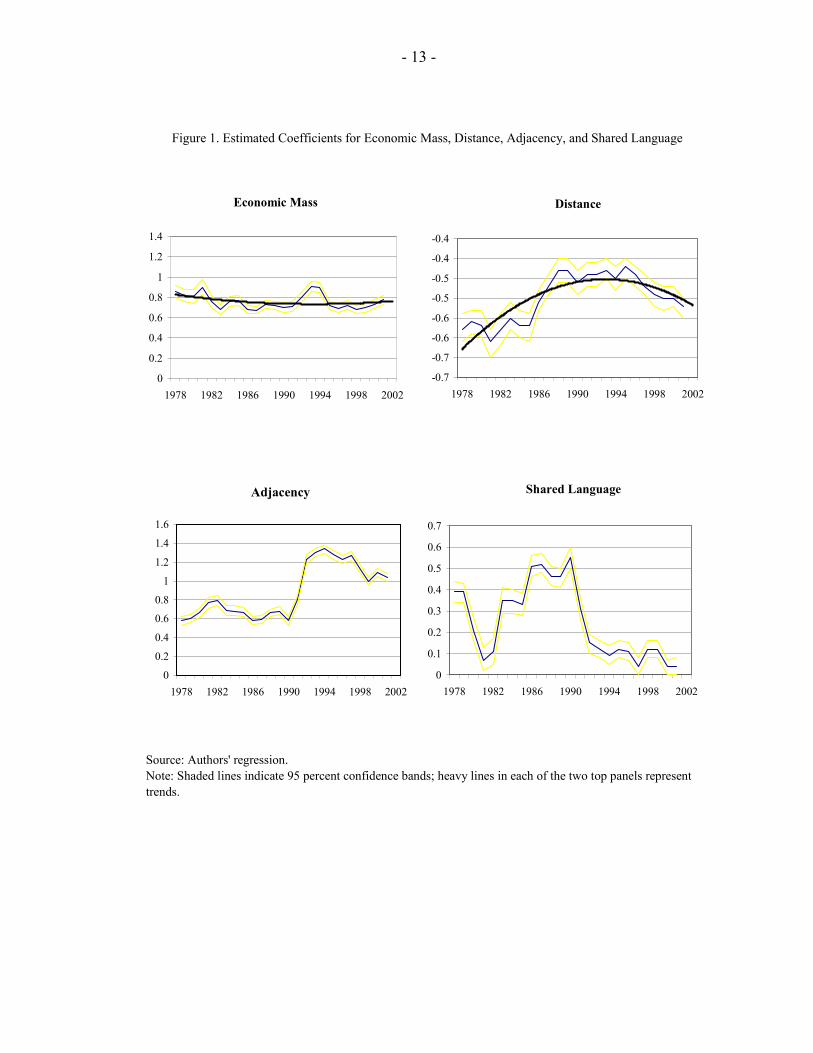
The nonlinear gravity model, equation (5), was estimated across selected countries for each year during 1978–2001. Table 1 reports the results of these estimations for selected years. The estimation results, based on nonlinear least squares, explain bilateral trade well, and most of the estimated coefficients have the expected sign. To better visualize and analyze the evolution of the recursively estimated coefficients, Figures 1 to 5 plot those results for each year during the sample period. The estimated coefficient on economic mass (the income elasticity of trade; top left panel of Figure 1) hovers around 0.8 (and is statistically significant for all years), from which we infer a value of –0.25 for the parameter η in equations (3) and (4). This implies that an increase in exports generates net negative externalities, which increase the trade cost factor and slow down further trade expansion. Through what channels these effects take place seems a promising avenue for research. We find that distance has become somewhat less relevant over time, as shown by the trend of the estimated distance coefficient in the top right panel of Figure 1. Although the estimated coefficients fell (in absolute value) over time from –0.57 (average of 1978–79) to –0.51 (average of 2000–01), their values still reveal the importance of geography in trade. A simple comparative static exercise, using our empirical equation (5), illustrates this point. Assume three countries A, B, and C; B and C are identical (same GDP, same country-specific variables), but at different distances from A and both trade with country A. Assume that the distance between A and C is three times greater than that between A and B. Using the estimated distance coefficient of –0.51 together with those assumptions, equation (5) yields the result that trade between A and C is equivalent to only 57 percent of trade between A and

11 It is not necessary to include the world GDP in equation 5 as suggested by equation 4, in view of the fact that we run a regression across the countries in our sample for each year. This variable, the world GDP, of course, does not vary across countries in a given year.

- 9 -

B. Thus, in spite of the technological progress experienced in the last two decades, global economic geography is still relevant. This represents one of the “puzzles of globalization.”12 To some extent our results on distance confirm the findings of CSTB. For example, those authors also find that the biggest change in the distance coefficient happened before the 1990s. However, CSTB’s distance coefficients are more volatile than ours and, unlike in our results, are highly correlated with the price of oil, which functions as a proxy for transportation costs. These differences might be due to the choice of data used to measure trade: CSTB use imports whereas we use exports.13 The coefficient for adjacency jumped in 1990 to a higher plateau, as shown in the bottom left panel of Figure 1. This may imply that neighboring countries trade more despite the fact that distance has become somewhat less relevant. Interestingly, the period during which adjacency became more relevant (the early 1990s) coincides with the surge in RTAs. Whereas during the 1980s there were only 10 RTAs worldwide, according to the WTO, since 1990 more than 100 new RTAs have been introduced. Because most RTAs were concluded among neighboring countries, regionalism does not necessarily contradict globalization and the reduced relevance of distance. The language coefficient, as shown in the bottom right panel of Figure 1, exhibits high volatility around a decreasing trend and takes a small positive value in 2001. It is not clear whether language captures only translation costs (and therefore the coefficient has declined as English has become more widespread) or also cultural unfamiliarity or something else. In any case our results show that language has recently become less important, and we suspect that future research will find the language variable to be irrelevant. Among the four main Western Hemisphere trading blocs, MERCOSUR, founded in 1991 by Argentina, Brazil, Paraguay, and Uruguay, has been relatively effective in reducing tariffs among its members, but it has had problems in coordinating the bloc’s external trade policy as envisioned in the agreement, let alone the other economic policies of its members. NAFTA superseded the Canada-United States Free Trade Agreement by adding a new member, Mexico, in 1994. The Andean Community received new attention in November 1990, when its members pledged to revive trade among themselves. However, the group soon suffered a setback when Peru unilaterally suspended the agreement in May 1992. The CACM, founded in 1961, has not made significant progress in the last two decades. 12 CSTB (2002, p. 3) define globalization as “the rapid increase in international trade spurred by advances in technology that have decreased the costs of trade over time.”

13 Both exports and imports have problems. Export data might not be available in some developing countries, whereas import data might be contaminated by the noise component of trade costs, in turn affected by movements in oil prices. This might explain the correlation that CSTB found between the estimated coefficient for distance and the oil price. Export data are free of the volatility induced by transportation costs, thus giving us a clearer picture of global trade.

- 10 -

An RTA might have an impact on trade either before (an “anticipation effect”) or after (a “lagging effect”) the official signing. An anticipation effect may arise when it takes a long time to negotiate a deal but there is a strong presumption that the deal will come to fruition. In these cases trade might increase even before the official inauguration. A lagging effect may arise when it takes a long time to implement the provisions of the treaty after its signing, possibly casting doubts about the seriousness of the agreement. Which effect dominates is an empirical matter, however. As a corollary, one should not necessarily expect a discontinuous jump in trade at the time the treaty becomes effective. The results for MERCOSUR are shown in Figure 2. As the top panel shows, the level of integration of the MERCOSUR countries has been increasing since the early 1980s, rather than beginning in the late 1980s as suggested by Yeats (1997). Our result seems more plausible, given that Argentina and Brazil (the largest MERCOSUR partners) signed 24 bilateral trade protocols between 1984 and 1988. The level of integration has leveled off since the mid-1990s (and has in fact decreased somewhat since 1998), which points to a lack of sustained integration among its members. The decline observed since 1998 might be due to macroeconomic shocks, such as the devaluation of the Brazilian real in January 1999. The propensity to import of MERCOSUR as a bloc, shown in the middle panel of Figure 2, decreased sharply after the early 1980s, coinciding with the start of the series of bilateral trade protocols between Argentina and Brazil mentioned above. It seems that the MERCOSUR countries have been closing their doors to the rest of the world. The bloc’s propensity to export, shown in the bottom panel of Figure 2, experienced a sharp increase in the 1980s, when the debt crisis-ridden countries increased exports to cope with the crisis. The PTE index continued its downward trend after the beginning of MERCOSUR and increased somewhat during the Argentine crises that started in mid-1988. The behavior of the propensities to import and export provides circumstantial evidence of trade diversion: countries divert imports and exports to their MERCOSUR partners. Interestingly, as shown in Table 1 and Figure 2, MERCOSUR’S propensities to import and export decreased and became significant precisely at the time when integration became significant. Thus integration and trade diversion went hand in hand in MERCOSUR. This probably reflects the overall trade liberalization of the MERCOSUR countries at the same time as they were forming the RTA among themselves. The results for NAFTA are shown in Figure 3. As illustrated in the top panel, in 1994, before the start of NAFTA, the coefficient for the level of integration was below zero.14 This coefficient started to increase after the mid-1980s coinciding with Mexico’s move toward trade liberalization at that time. This upward trend reversed following the 1990 pre-NAFTA 14 This result, which is consistent with previous research, would seem to indicate that NAFTA was not a natural trading bloc. However, this is not necessarily the case, because Mexico in that period was a relatively closed economy (an import substitution scheme had been in place there since the late 1940s, as in most countries in Latin America), and Mexican exports were dominated by oil.

- 11 -

agreement between Mexico and the United States, but the coefficient began to trend upward again following the official signing of NAFTA in 1994. After 1990 there were some doubts about whether to proceed with NAFTA (there was political opposition from interest groups and from some legislators in the United States) as well as doubts about the permanence of the Mexican trade reforms. These doubts, which were dispelled after NAFTA was signed, might have played a role in the temporary reversal of the upward trend of the estimated coefficient for the level of integration. It is not easy to draw definite conclusions from the behavior of the propensities to import and export, shown in the bottom two panels of Figure 3. One might perceive some weak indication of trade diversion when comparing the values of these indices during the 1990s versus the 1980s. The results for the CACM are shown in Figure 4. The estimated coefficient for the level of integration has remained flat and statistically not significantly different from zero during the last two decades, confirming the perception that integration in this region never took off. During the same period the propensity to export has also remained flat, at a level not significantly different from zero, and the propensity to import dropped in the early 1980s only to start increasing again in the late 1980s. Thus the evidence for CACM points to trade diversion without further integration. The results for the Andean Community are shown in Figure 5. The estimated coefficient for the level of integration of this group increased precisely around the time of the group’s revival in November 1990; however, the coefficient continues to be insignificant until 1994. Furthermore, the increase seems to be a one-time phenomenon. The propensities to export and to import both decreased at around the same time, showing some evidence of trade diversion. Thus the evidence for the Andean Community points to more trade diversion than integration.

- 12 -

1978

1980

1983

1986

1989

1992

1995

1998

2001

Econ

omic

mas

s0.

86**

0.81

**0.

68**

0.68

**0.

72**

0.80

**0.

72**

0.68

**0.

77**

Popu

latio

n - E

xpor

t Cou

ntry

0.14

**0.

26**

0.35

**0.

35**

0.41

**0.

32**

0.39

**0.

51**

0.36

**Po

pula

tion

- Im

port

Cou

ntry

0.20

**0.

32**

0.51

**0.

52**

0.44

**0.

38**

0.49

**0.

59**

0.52

**D

ista

nce

-0.5

8**

-0.5

7**

-0.5

5**

-0.5

1**

-0.4

3**

-0.4

4**

-0.4

2**

-0.4

9**

-0.5

2**

Adj

acen

cy0.

58**

0.66

**0.

69**

0.58

**0.

68**

1.23

**1.

28**

1.12

**1.

04**

Lang

uage

0.39

**0.

21**

0.35

**0.

51**

0.46

**0.

15**

0.12

**0.

12**

0.04

**

ME

RC

OSU

R:

Leve

l of I

nteg

ratio

n0.

090.

160.

291.

18*

1.77

**1.

29**

1.72

**2.

08**

1.57

**B

loc's

pro

pens

ity to

Impo

rt0.

33*

0.24

0.45

0.17

-0.7

4*

-0.7

6**

-0.8

4**

-1.0

0**

-0.6

0**

Blo

c's p

rope

nsity

to E

xpor

t0.

08-0

.68

**0.

56*

0.23

-0.5

6*

-0.6

4**

-1.1

5**

-1.2

6**

-0.5

6**

NA

FTA

:Le

vel o

f Int

egra

tion

-0.2

3*

0.06

-0.1

2-0

.32

**-0

.06

-0.1

6*

0.07

0.28

**0.

37**

Blo

c's p

rope

nsity

to Im

port

0.29

0.09

1.07

*1.

32**

0.57

0.07

0.04

-0.2

5*

-0.3

5**

Blo

c's p

rope

nsity

to E

xpor

t0.

12-0

.39

*0.

66*

0.87

**0.

07-0

.09

-0.0

9-0

.15

-0.2

2

CA

CM

:Le

vel o

f Int

egra

tion

3.33

*3.

50*

2.68

1.14

1.67

1.97

2.23

1.53

1.44

Blo

c's p

rope

nsity

to Im

port

0.13

0.06

-1.7

2**

-2.4

1**

-2.1

7**

-2.1

1**

-1.8

4**

-1.5

5**

-1.6

5**

Blo

c's p

rope

nsity

to E

xpor

t0.

730.

420.

750.

730.

350.

42-0

.05

0.62

1.05

**

AN

DE

AN

:Le

vel o

f Int

egra

tion

-0.2

4-0

.12

0.33

0.45

0.83

1.08

1.91

*1.

86*

1.58

*B

loc's

pro

pens

ity to

Impo

rt1.

27**

1.05

**1.

45**

0.41

**0.

640.

78**

0.23

0.03

-0.0

4B

loc's

pro

pens

ity to

Exp

ort

0.94

**0.

59**

1.08

**0.

85**

0.75

**0.

74**

0.19

0.05

0.54

**

Num

ber o

f obs

erva

tions

3,90

93,

848

3,97

43,

991

4,00

54,

010

4,01

44,

017

4,01

7A

djus

ted

R2

0.95

0.93

0.94

0.97

0.96

0.95

0.96

0.97

0.97

Sour

ce: O

wn

calc

ulat

ion.

1 Tra

de is

def

ined

usi

ng p

artn

er c

ount

ry e

xpor

t dat

a (T

ij =

Xij

+ X

ji); *

and

**

indi

cate

coe

ffic

ient

s sig

nific

antly

diff

eren

t fro

m z

ero

at th

e 5

and

1pe

rcen

t lev

el, r

espe

ctiv

ely.

(dep

ende

nt v

aria

ble:

trad

e; 6

4 ec

onom

ies,

1978

–200

1) 1

Tabl

e 1:

Est

imat

ed C

oeff

icie

nts o

f the

Non

linea

r Cos

t-Cor

rect

ed G

ravi

ty M

odel

- 13 -

Economic Mass

0

0.2

0.4

0.6

0.8

1

1.2

1.4

1978 1982 1986 1990 1994 1998 2002

Distance

-0.7

-0.7

-0.6

-0.6

-0.5

-0.5

-0.4

-0.4

1978 1982 1986 1990 1994 1998 2002

Adjacency

0

0.2

0.4

0.6

0.8

1

1.2

1.4

1.6

1978 1982 1986 1990 1994 1998 2002

Shared Language

0

0.1

0.2

0.3

0.4

0.5

0.6

0.7

1978 1982 1986 1990 1994 1998 2002

Source: Authors' regression.Note: Shaded lines indicate 95 percent confidence bands; heavy lines in each of the two top panels represent trends.

Figure 1. Estimated Coefficients for Economic Mass, Distance, Adjacency, and Shared Language

- 14 -

Figure 2. MERCOSUR: Estimated Gravity Model Coefficients

Level of Integration

-1.5

-0.5

0.5

1.5

2.5

3.5

1978 1982 1986 1990 1994 1998 2002

Propensity to Import

-1.5-1.0-0.50.00.51.01.52.0

1978 1982 1986 1990 1994 1998 2002

Propensity to Export

-1.5-1.0-0.50.00.51.01.52.0

1978 1982 1986 1990 1994 1998 2002

Source: Authors' regressions.Note: Shaded lines indicate 95 percent confidence bands; heavy line in the top panel represents the trend.

- 15 -

Figure 3. NAFTA: Estimated Gravity Model Coefficients

Source: Authors' regressions.Note: Shaded lines indicate 95 percent confidence bands; heavy line in the top panel represents the trend.

Level of Integration

-0.6-0.4-0.2

00.20.40.60.8

1978 1982 1986 1990 1994 1998 2002

Propencity to Import

-1-0.5

00.5

11.5

22.5

1978 1982 1986 1990 1994 1998 2002

-1

-0.5

0

0.5

1

1.5

1978 1982 1986 1990 1994 1998 2002

Propensity to Export

- 16 -

Figure 4. CACM: Estimated Gravity Model Coefficients

Level of Integration

-15-10-505

101520

1978 1982 1986 1990 1994 1998 2002

Propensity to Import

-3

-2

-1

0

1

2

1978 1982 1986 1990 1994 1998 2002

Propensity to Export

-2

-1

0

1

2

3

1978 1982 1986 1990 1994 1998 2002

Source: Authors' regressions.Note: Shaded lines indicate 95 percent confidence bands; heavy lines represent trends.

- 17 -

Figure 5. Andean Community: Estimated Gravity Model Coefficients

Level of Integration

-4.5

-2.5

-0.5

1.5

3.5

5.5

1978 1982 1986 1990 1994 1998 2002

Propensity to Import

-1-0.5

00.5

11.5

22.5

3

1978 1982 1986 1990 1994 1998 2002

Propensity to Export

-0.5

0

0.5

1

1.5

2

1978 1982 1986 1990 1994 1998 2002

Source: Authors' regressions.Note: Shaded lines indicate 95 percent confidence bands; heavy lines represent trends.

- 18 -

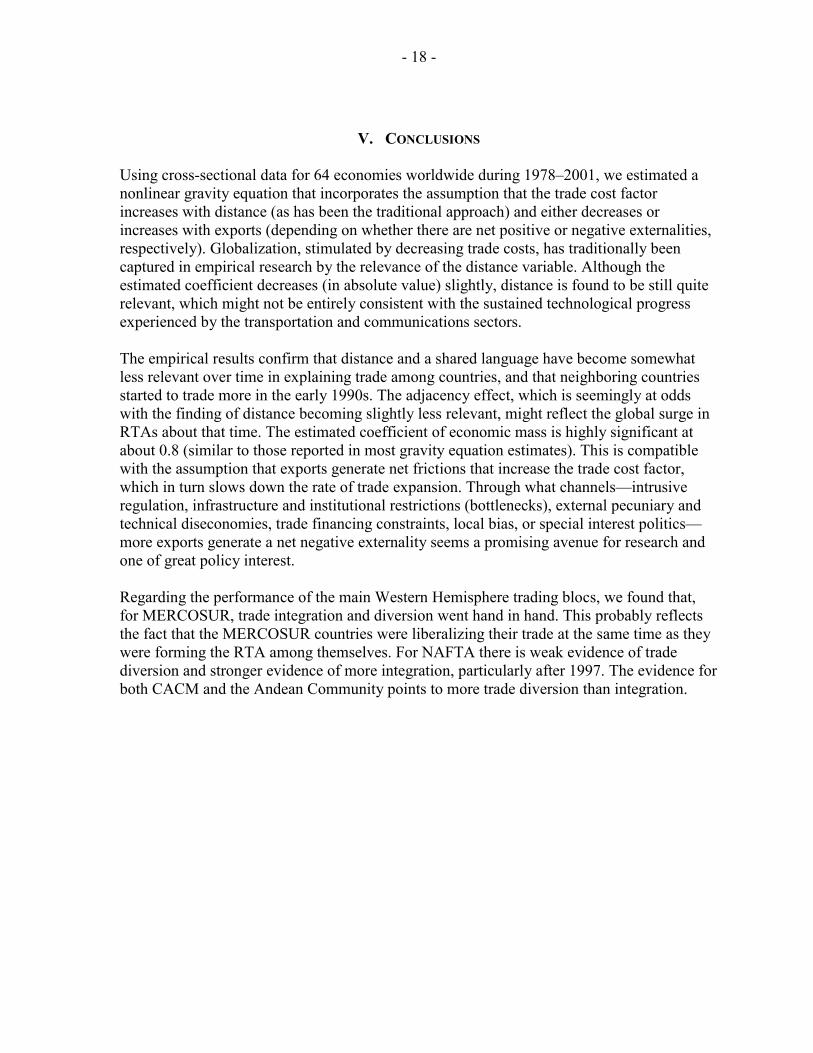
V. CONCLUSIONS Using cross-sectional data for 64 economies worldwide during 1978–2001, we estimated a nonlinear gravity equation that incorporates the assumption that the trade cost factor increases with distance (as has been the traditional approach) and either decreases or increases with exports (depending on whether there are net positive or negative externalities, respectively). Globalization, stimulated by decreasing trade costs, has traditionally been captured in empirical research by the relevance of the distance variable. Although the estimated coefficient decreases (in absolute value) slightly, distance is found to be still quite relevant, which might not be entirely consistent with the sustained technological progress experienced by the transportation and communications sectors. The empirical results confirm that distance and a shared language have become somewhat less relevant over time in explaining trade among countries, and that neighboring countries started to trade more in the early 1990s. The adjacency effect, which is seemingly at odds with the finding of distance becoming slightly less relevant, might reflect the global surge in RTAs about that time. The estimated coefficient of economic mass is highly significant at about 0.8 (similar to those reported in most gravity equation estimates). This is compatible with the assumption that exports generate net frictions that increase the trade cost factor, which in turn slows down the rate of trade expansion. Through what channels—intrusive regulation, infrastructure and institutional restrictions (bottlenecks), external pecuniary and technical diseconomies, trade financing constraints, local bias, or special interest politics—more exports generate a net negative externality seems a promising avenue for research and one of great policy interest. Regarding the performance of the main Western Hemisphere trading blocs, we found that, for MERCOSUR, trade integration and diversion went hand in hand. This probably reflects the fact that the MERCOSUR countries were liberalizing their trade at the same time as they were forming the RTA among themselves. For NAFTA there is weak evidence of trade diversion and stronger evidence of more integration, particularly after 1997. The evidence for both CACM and the Andean Community points to more trade diversion than integration.

- 19 - APPENDIX I

APPENDIX

I. Data Descriptions We use a sample of 64 industrial and developing economies (listed in Table 2) for the period 1978–2001. Nominal GDP and GDP per capita (both in dollars), and population are from the IMF’s World Economic Outlook Database. Bilateral trade data between pairs of countries (exports from country i to country j) in dollars are from the IMF’s Direction of Trade Database. The definition of trading bloc is taken from WTO (2000). We use the same sample of economies as in Frankel and Wei (1993) with some modifications: We omitted South Africa and Belgium (because of lack of data and technical reasons), and we added several Latin American countries because this region is the focus of our research. Our sample starts in 1978 because three countries dropped out of the sample between 1977 and 1978 (these countries represent just 10 percent of the observations in the sample). The data for the language and adjacency variables were generously provided by CSTB. The data for distance—defined for each country pair as the distance between their capitals—were obtained from the Centre d'Etudes Prospectives et d'Informations Internationales (www.cepii.fr/anglaisgraph/bdd/distances.htm).

Table 2. Sample of 64 Economies

Algeria Argentina Australia Austria Bolivia Brazil Canada Chile China Colombia Costa Rica Denmark Ecuador

El Salvador Egypt Ethiopia Finland France Germany Ghana Greece Guatemala Honduras Hong Kong SAR Hungary Iceland

India Indonesia Iran, I.R. of Ireland Israel Italy Japan Kenya Korea Kuwait Libya Malaysia Mexico

Morocco The Netherlands New Zealand Nicaragua Nigeria Norway Pakistan Paraguay Philippines Peru Poland Portugal Saudi Arabia

Singapore Spain Sudan Sweden Switzerland Thailand Tunisia Turkey United Kingdom United States Uruguay Venezuela

- 20 - APPENDIX II

II. The Trade Cost Factor and the Volume of Trade, and the Cost of Bilateral Resistance

A general specification of the trade cost factor, widely used in the literature, is:

ij ijt b d ρ= × , where dij stands for distance and b is a parameter capturing other types of frictions. Under this specification of the trade cost factor, the gravity equation exhibits unitary income elasticity (that is, the elasticity of exports with respect to the relative economic mass equals one). However, most empirical research has found an income elasticity larger than zero but less than one. To reconcile the empirical findings with the theory, we propose a novel specification of the trade cost factor:

( )

( )

/ 1

/ 1ij

ijij

dt

X

β σ

η σ

−

− −= ,

where Xij represents exports from country i to country j, 1 – σ < 0, β < 0, and –1 < η < 1. This trade cost factor between two countries depends, as usual, on the distance separating them, but also on the volume of trade between those countries. The greater the distance, the higher the trade cost factor; and more trade produces externalities that might either increase or decrease the trade cost factor. More exports from country i to j would reduce tij if 0 < η < 1 and increase it if –1 < η < 0. Positive externalities increase trade by reducing the trade cost factor through learning by doing, sunk costs, networks, or external pecuniary and technical economies. Negative externalities slows down the increase in trade by increasing the trade cost factor through infrastructure and institutional restrictions, trade financing constraints, technical diseconomies, or opposition to trade from special interest groups. Which type of externality dominates is an empirical issue, but one that policies could affect. Substituting the trade cost factor in the gravity equation, we obtain

1111

11i jij ijw

i j

GDP GDPX d

GDP P P

σβηηη

−−−

− ×

= × .

The restriction that η take values between –1 and 1 implies that 1 – η > 0. Thus this modified gravity equation states that trade between two countries will be higher, the shorter is the distance between them, the higher the multilateral resistance of either of those countries to trade with the rest of the world, and the greater the economic mass of those countries relative to the rest of the world. Note that our specification of the trade cost factor implies an income elasticity of the gravity equation of 1/(1 – η), which is larger than one if positive externalities dominate, smaller than

- 21 - APPENDIX II

one (but larger than zero) if negative externalities dominate, or equal to one if the positive and negative externalities exactly offset each other. We define the cost of bilateral resistance between countries i and j as the trade that is lost because of that bilateral resistance, as a proportion of the countries’ relative economic mass. Concretely, the difference between the volume of trade that would obtain in the absence of bilateral frictions (that is, tij = 1) and the actual volume of trade, divided by their relative economic mass, is

ij ij

i jw

X XC GDP GDP

GDP

−=

×,

where

11i j

ij wi j

GDP GDPX

GDP P P

σ− ×

= × .

Thus, using the above two definitions and the gravity equation, we obtain

1111

11 1i jijw

i j i j

GDP GDPC d

P P P PGDP

σησ βηηη

−−

−−−

× = − × ×

,

with

0Cd

∂>

∂

i jw

CGDP GDP

GDP

∂×

∂

< 0 (if 0 < η < 1), or > 0 (if –1 < η < 0).

Finally, ( )i j

CP P∂

∂ × is either greater than or less than zero, depending on the values of the

parameters σ and η, as well as the other variables included in the cost function.

- 22 -

REFERENCES Anderson, James E. 1999, “Why do Nations Trade (So Little)?” Mimeograph (August),

Boston College. Anderson, James E., and Eric Van Wincoop, 2003, “Gravity with Gravitas: A Solution to the

Border Puzzle,” American Economic Review, Vol. 92 (March), pp. 170–92. Bernard, Andrew B., and Joachim Wagner, 1998, “Export Entry and Exit by German Firms,”

National Bureau of Economic Research Working Paper Series No. 6538 (Cambridge, Massachusetts: National Bureau of Economic Research).

Coe, David T., Arvind Subramanian, Natalia T. Tamirisa, and Tikhil Bhavnani, 2002, “The

Missing Globalization Puzzle,” IMF Working Paper WP/02/171 (Washington: International Monetary Fund).

Dell’Ariccia, Giovanni, 1999, “Exchange Rate Fluctuations and Trade Flows: Evidence from

the European Union,” IMF Staff Papers, 46, No. 3 (September–December), pp. 315–34.

Edwards, Sebastian, 1995, Crisis and Reform in Latin America: From Despair to Hope (Washington: World Bank and Oxford University Press).

Ethier, Wilfred J., 1998, “Regionalism in a Multilateral World,” Journal of Political

Economy, Vol. 106, No. 6 (December), pp. 1214–45. Frankel, Jeffrey A. (with Ernesto Stein and Shang Jin Wei), 1997, Regional Trading Blocs in

the World Economic System (Washington: Institute for International Economics). ———, and Shang-Jin Wei, 1993, “Is There a Currency Bloc in the Pacific?” CIDER

Working Paper No. C93-025 (Berkeley, California: University of California, Center for International and Development Economics Research).

Glick, Reuven, 1998, “Contagion and Trade: Why Are Currency Crises Regional?” National

Bureau of Economic Research Working Paper No. 6806 (Cambridge, Massachusetts: National Bureau of Economic Research).

Krueger, Anne O., 1999, “Trade Creation and Trade Diversion Under NAFTA,” National

Bureau of Economic Research Working Paper No. 7429 (Cambridge, Massachusetts: National Bureau of Economic Research).

Obstfeld, Maurice, and Kenneth Rogoff, 2000, “The Six Major Puzzles in International

Macroeconomics: Is There a Common Cause?” National Bureau of Economic Research Working Paper No. 7777 (Cambridge, Massachusetts: National Bureau of Economic Research).

- 23 -

Panagariya, Arvind, 1999, “The Regionalism Debate: An Overview,” World Economy, Vol. 4 (June), pp. 477–511.

Roberts, Mark J., and James R. Tybout, 1997, “The Decision to Export in Colombia: An

Empirical Model of Entry with Sunk Costs,” American Economic Review, Vol. 87 (September), pp. 545–64.

Soloaga, Isidro, and L. Alan Winters, 1999, “Regionalism in the Nineties: What Effect on

Trade?” Centre for Economic Policy Research Discussion Paper Series No. 2183 (London: Centre for Economic Policy Research).

Summers, Lawrence, 1993, “Regionalism and the World Trading System,” In Policy

Implications of Trade and Currency, Proceedings of a Symposium Sponsored by the Federal Reserve Bank of Kansas City, Jackson Hole, Wyoming (Kansas City, Missouri: Federal Reserve Bank of Kansas City).

World Bank, 2000, “Trade Blocs and Beyond: Political Dreams and Practical Decisions,”

Policy Research Report (Washington). World Trade Organization, 2000, “Mapping of Regional Trade Agreements” (October). Yeats, Alexander J., 1997, “Does MERCOSUR’S Trade Performance Raise Concerns About

the Effects of Regional Trade Arrangements?” Policy Research Working Paper 1729 (Washington: World Bank).