PARALLEL MULTISCALE GAUSS-NEWTON-KRYLOV METHODS FORINVERSE WAVE PROPAGATION �

VOLKAN AKCELIK y, GEORGE BIROSz, AND OMAR GHATTASx

Abstract. One of the outstanding challenges of computational science and engineering is large-scale nonlinearparameter estimation of systems governed by partial differential equations. These are known asinverse problems, incontradistinction to theforward problemsthat usually characterize large-scale simulation. Inverse problems are sig-nificantly more difficult to solve than forward problems, due to ill-posedness, large dense ill-conditioned operators,multiple minima, space-time coupling, and the need to solve the forward problem repeatedly. We present a paral-lel algorithm for inverse problems governed by time-dependent PDEs, and scalability results for an inverse wavepropagation problem of determining the material field of an acoustic medium. The difficulties mentioned above areaddressed through a combination of total variation regularization, preconditioned matrix-free Gauss-Newton-Kryloviteration, algorithmic checkpointing, and multiscale continuation. We are able to solve a synthetic inverse wavepropagation problem though a pelvic bone geometry involving 2.1 million inversion parameters in 3 hours on 256processors of the Terascale Computing System at the Pittsburgh Supercomputing Center.

1. Computational challenges in large-scale inverse problems.One of the outstandingchallenges of computational science and engineering is large-scale parameter estimation ofsystems governed by partial differential equations (PDEs). These are known asinverse prob-lems, and are distinguished from theforward problemsthat usually characterize large-scalesimulations. In the forward problem, the PDE parameters—initial conditions, boundary anddomain sources, material coefficients, and the domain geometry—are known, and the stateof the system is determined by solving the PDEs. The inverse problem reverses the process:some components of the state are observed, while some subset of PDE parameters is un-known. An objective function that minimizes the differences between the observed states andthose predicted by the PDEs is formulated, and solution of a nonlinear optimization problemyields components of the unknown parameters.

The inverse problem is often significantly more difficult to solve than the forward prob-lem, because:

� forward solution is just a subproblem of the inverse problem;� the inverse problem is often ill-posed despite the well-posedness of the forward

problem;� the inverse operator couples the entire time history of the system’s response, as op-

posed to the usual case with forward evolution operators; and� the inverse problem can have numerous local solutions.

Not surprisingly, most of the work in large-scale simulation has been directed at the forwardproblem. But sustained advances over the past 20 years have produced a body of efficient,

�This work supported by the National Science Foundation’s Knowledge and Distributed Intelligence (KDI) andInformation Technology Research (ITR) programs (through grants CMS-9980063 and ACI-0121667), the Depart-ment of Energy’s Scientific Discovery through Advanced Computation (SciDAC) program through the TOPS Center,and the Computer Science Research Institute at Sandia National Laboratories. Computing resources on the Cray T3Eand Compaq TCS systems are provided by the Pittsburgh Supercomputing Center under awards ASC-010025P andASC-010036P.

yMechanics, Algorithms, and Computing Laboratory, Department of Civil & Environmental Engineering,Carnegie Mellon University, Pittsburgh, Pennsylvania, 15213, USA (volkan@cs.cmu.edu ).

zCourant Institute, for Mathematical Sciences, New York University, New York, NY, 10012, USA(biros@cs.nyu.edu )

xMechanics, Algorithms, and Computing Laboratory, Departments of Biomedical Engineering and Civil& Environmental Engineering, Carnegie Mellon University, Pittsburgh, Pennsylvania, 15213, USA (oghat-tas@cs.cmu.edu ).

0-7695-1524-X/02 $17.00 (c) 2002 IEEE

1

2 A. AKCELIK, G. BIROS, AND O. GHATTAS

parallel, and scalable algorithms for many classes of forward PDE simulations, inviting pur-suit of the more challenging problem of inversion.

However, designing scalable parallel numerical algorithms for the solution of nonlinearPDE-based inverse problems poses a significant challenge. This is particularly true for large-scale inverse problems, in which the number of inversion parameters is mesh-dependent (forexample when the parameters represent unknown initial conditions, distributed sources, orheterogeneous material properties). In this case, scalability—both to large problem sizesand large numbers of processors—is crucial. Newton’s method—the archetypical scalablenonlinear solver—entails a number of difficulties for such problems:

� The Hessian matrices required by Newton’s method are (formally) dense and of theorder of the number of inversion parameters, and their construction involves numer-ous solutions of the forward problem. Thus, straightforward implementations forgrid-based parameterizations require prohibitive memory, work, and communica-tion.

� The denseness, large size, and difficulty of construction of the linearized inverseoperators rule out direct solvers. For the same reasons, matrix-based iterative solversare not practical. On the other hand, matrix-free implementations can be made toexploit problem structure, so that each matrix-vector product requires solution ofjust a few forward-like PDE problems. However, this freedom from having to forma matrix creates difficulties in constructing a preconditioner, which is essential whenmore sophisticated regularizers are used to produce a well-posed inverse problem.

� Objective functions for nonlinear inverse problems are often nonconvex; Newton’smethod will likely diverge without careful attention to globalization. Worse, formany nonlinear inverse problems, the objective functions to be minimized may havemany local minima. In particular, for the inverse wave propagation problems tar-geted in this paper, they are highly oscillatory, with basins of attraction that shrinkwith the wavelength of the propagating waves. General-purpose global optimiza-tion methods are incapable of scaling to the large numbers of inversion parametersinduced by grid-based parameterizations. On the other hand, local methods likeNewton’s become trapped at local minima unless the objective function can be con-vexified.

Given the above difficulties faced by Newton-like methods, it is not surprising that manylarge-scale PDE inverse methods are based on gradients alone and avoid Hessian matrices.The simplest such techniques are steepest descent-type methods, in which the current solu-tion is improved by moving in the direction of the negative gradient of the objective function.Better directions can be constructed, still based on gradient information, via nonlinear con-jugate gradient (CG) methods. Even better are limited memory quasi-Newton methods (suchas L-BFGS), which build a limited amount of curvature information based on changes in thegradient, and reduce to nonlinear CG in certain limiting cases. All of these gradient-basedmethods avoid the difficulties brought on by large dense Newton Hessians mentioned above.Moreover, their parallel efficiency can be high, since the gradient computation involves PDE-like solves, for which there exists a large body of parallel algorithms and libraries on which todraw. However, unlike Newton methods, they do not scale well with increasing problem size,suffering a reduction from quadratic to linear asymptotic convergence, and perform poorlyfor ill-conditioned problems. Nevertheless, for moderately-sized problems (in both parame-ter and state spaces), they offer a reasonable compromise between performance and ease ofimplementation, and this explains their popularity.

However, there is a desire to solve ever-larger inverse problems in such areas as globalclimate change, weather forecasting, ocean modeling, air and groundwater pollutant trans-

PARALLEL INVERSE WAVE PROPAGATION 3

port, earthquake modeling, astrophysics, hazardous substance attacks, non-destructive mate-rials testing, medical imaging, electromagnetic sensing, turbulence modeling, reservoir simu-lation, and so on. In many of these areas, increasing confidence in the fidelity of PDE models,combined with the greater power of PDE solvers and computing hardware, have resulted inPDE simulations that are sufficiently predictive to invite inversion of highly-resolved andhighly-parameterized models. For these large-scale problems, linearly convergent methodssuch as L-BFGS are usually not viable; instead we need algorithms that are scalable, bothwith increasing problem size and numbers of processors.

In this paper we present and assess the scalability of a parallel algorithm for time-domainPDE-based inverse problems. The target application is 3D inverse wave propagation, inwhich the goal is to determine coefficients of the material parameter field of a heterogeneousmedium, given a source and waveform observations at receiver locations on its boundary.Inverse problems of this type arise in seismic exploration, earthquake modeling, ultrasoundimaging, matched field processing, ocean acoustics, treaty verification, obstacle detection,nondestructive evaluation, and structural health monitoring. We present results for inversionof the velocity field of a scalar linear wave equation, which is representative of this classof inverse wave propagation problems and contains the major difficulties of rank-deficiency,ill-conditioning, large-scale, space-time coupling, and numerous local minima with basins ofattraction that shrink with increasing frequency of propagating waves.

Because many of the inverse wave propagation problems of interest are “100-wavelengthproblems,” i.e. there is a desire to reconstruct feature sizes that are several hundred times finerthan characteristic dimensions, is it essential that inversion algorithms be able to scale tothousand-grid-point resolution in each spatial dimension, which for heterogeneous 3D prob-lems results in billion-parameter inverse problems. For example, one of our target problems isthe estimation of the elastic mechanical properties (Lam´e moduli and density) of the greaterLos Angeles Basin, given seismograms of past earthquakes in the region, an elastic wavepropagation forward model, and models of the seismic sources. Terascale (and beyond) com-puting is needed for such large-scale problems, and thus scalability to large processor countsis essential.

To treat multiple local minima, we employ multiscale continuation, in which a sequenceof initially convex, but increasingly oscillatory, approximations to the objective function areminimized over a sequence of increasingly finer discretizations of state and parameter spaces,which in our experience keeps the sequence of minimizers within the basin of attraction of theglobal minimum. Total variation regularization is used to address ill-posedness and preservesharp interfaces in the inversion parameter space. To overcome the difficulties of large, dense,expensive-to-construct, indefinite Newton Hessians, we combine Gauss-Newton linearizationwith matrix-free inner Krylov iterations. These require good preconditioners in the case ofthe total variation regularization operator, which presents considerable difficulties due to itsstrong heterogeneity and anisotropy. Our preconditioner is based on the L-BFGS algorithmto approximate curvature information using changes in directional derivatives, initialized bysecond order stationary iterations applied to the total variation operator.

All of these computational components require linear work and parallelize well in adomain-based manner (i.e. fine granularity parallelism induced by a partition of the mesh).The remaining requirement for assuring overall scalability is mesh-independence of (or morerealistically weak dependence on) the outer nonlinear and inner linear iterations. Newtonmethods often deliver mesh-independence for nonlinear operators for sufficiently-fine grids,and appropriately preconditioned inverse operators can produce spectra that are favorable forKrylov methods. However the total variation operator becomes increasingly ill-conditionedwith decreasing mesh size, which often results in an increase of Newton iterations with mesh

4 A. AKCELIK, G. BIROS, AND O. GHATTAS

size. In this paper we study the performance of our algorithm with respect to these scalabilityissues in the context of the inverse wave propagation problem.

We begin in Section 2 by formulating the inverse problem as a PDE-constrained opti-mization problem. In Section 3, we present the Newton-Krylov method, in infinite-dimen-sional strong form for simplicity of presentation. In Section 4, we give numerical results onthe Terascale Computing System (TCS) at the Pittsburgh Supercomputing Center (PSC), anddraw conclusions.

2. Inverse heterogeneous wave propagation.In this section, we formulate the inversewave propagation problem as a problem in PDE-constrained optimization, and derive the firstorder necessary conditions that characterize its solution. The optimization approach to a gen-eral form of this inverse problem was first elaborated by Tarantola [14]. Consider an acousticmedium with domain and boundary�. The medium is excited with a known acoustic en-ergy sourcef(x; t) (for simplicity we assume a single source event), and the pressureu�(x; t)is observed atNr receivers, corresponding to pointsxj in the domain. Our objective is to inferfrom these measurements the squared acoustic velocity distributionq(x), which is a propertyof the medium. From now on we refer toq as the material model andu(x; t) as the state vari-able. We can formulate the inverse problem as a nonlinear least squares parameter estimationproblem with PDE constraints. We seek to minimize, over the periodt = 0 to T , anL2 normdifference between the observed state and that predicted by the PDE model of acoustic wavepropagation, at theNr receiver locations. The PDE-constrained optimization problem is:

minu;q

1

2

NrXj=1

Z T

0

Z

[u� � u]2Æ(x � xj) d dt+ �F(q)

subject to �u�r � qru = f in � (0; T ]

qru � n = 0 on �� (0; T ](2.1)

u = _u = 0 in � ft = 0g

The first term in the objective function is the misfit between observed and predicted states,the second term�F(q) symbolizes the regularization functional with regularization param-eter�, and the constraints are the initial–boundary value problem for acoustic wave prop-agation./footnoteThe form in which the acoustic equation is given assumes a constant bulkmodulus and variable density; our method is equally applicable to a variable bulk modulusand constant density, or the case when both are variable. Here we have chosen zero initialconditions and Neumann boundary conditions, but the algorithms we discuss in this paperextend to more general conditions (as well as more general wave propagation PDEs).

In the absence of regularization, the problem as formulated above is ill-posed: the solu-tion may not be unique nor depend continuously on the given data [12]. Discretization of theinverse problem leads to inverse operators that are ill-conditioned and rank deficient. The nullspace of the inversion operator contains high frequency components of the material modelq,which cannot be determined from the band-limited responseu. Moreover, certain regionsof the medium may be “hidden” as a result of source/receiver density and location, furtherenlarging the null space of the inverse operator. One remedy is to regularize with theL2 normof the gradient of the material model,

F(q) =�

2

Z

rq � rq d

SuchTikhonovregularization eliminates the null space by penalizing oscillatory componentsof q; the more oscillatory, the greater the damping of those components. The effect becomes

PARALLEL INVERSE WAVE PROPAGATION 5

more pronounced with larger values of�, which must be chosen large enough to damp outfrequency components ofq that are larger than those justified by the observationsu�, butnot too large that true information is lost. See [15, Ch.7] for a discussion of techniques forchoosing the value of�.

Tikhonov regularization will smooth discontinuities in the material modelq, and is thusinappropriate for inverse problems with sharp interfaces, for example those between boneand soft tissue, sedimentary basin and rock, concrete and rebar, ocean water and sediment, oracross cracks. For such problems, in (2.1) we choose the total variation (TV) regularizationfunctional

FTV (q) = �

Z

jrqj" d;

where

jrqj" = (rq � rq + ")1

2 :

FTV is the bounded variation seminorm of the material model, modified by the parameter".The addition of" makes the regularization term differentiable. TV regularization effectivelypreserves (line in 2D, surface in 3D) jump discontinuities inq, since the TV functional, un-like Tikhonov, is bounded in this case; at the same time, it damps out spurious oscillationsin smooth regions [1]. The tradeoff is that the discrete TV operator is very ill-conditioned; itis effectively a nonlinear Poisson operator with widely-varying and highly anisotropic coef-ficient. For both Tikhonov and TV, we assumerq � n = 0 on�, i.e. the material model doesnot change in the normal direction on the boundary.

However, regularization does not cure all the problems. In addition to the null space prob-lems described above, the objective function can be highly oscillatory in the space of materialmodelq. Thus, there can be many local minima to contend with. Moreover, this oscillatorybehavior becomes more pronounced with increasing frequency of propagating waves: the di-ameter of the basin of attraction of the global minimum varies as their wavelength, and localoptimization methods become increasingly doomed to failure [13, 7].

To overcome this problem, we use multilevel grid and frequency continuation to generatea sequence of solutions that remain in the basin of attraction of the global minimum; that is,we solve for increasingly higher frequency components of the material model, on a sequenceof increasingly finer grids with increasingly higher frequency sources [6]. Figure 2.1 showsan example of the TV-regularized solution of a synthetic inverse wave propagation problem,and the ability of multiscale continuation to keep Newton’s method in the basin of attractionof the global minima. Note the sharp resolution of reconstructed interfaces on the finest grid(second-to-last frame). Figure 2.2 illustrates the effect of multiscale continuation and TVregularization. Without multiscale continuation, the optimization algorithm becomes trappedin a local minimum (Frame B) far from the global optimium. Frame C demonstrates thesmoothing of interfaces due to the use of TikhonovH1 seminorm regularization.

The equations that determine the solution to the optimization problem (2.1) can be de-rived by requiring stationarity of aLagrangian functional. These so-called optimality con-ditions take the form of a coupled nonlinear three-field system of integro-partial-differentialequations in the state variableu, theadjointvariable�, and the material modelq:

�u�r � qru = f in � (0; T ];

qru � n = 0 on �� (0; T ];(2.2)

u = _u = 0 for � ft = 0g;

6 A. AKCELIK, G. BIROS, AND O. GHATTAS

FIG. 2.1. Inversion of a piecewise-homogeneous material model corresponding to three circular scatterersusing TV regularization. Receiver locations on top, sources on bottom, receiver data is synthesized based on forwardsolution of target model shown in last (naturally-ordered) frame. Initial guess is a homogeneous medium with a singleparameter; increasingly finer inversion models are computed on increasingly finer grids, with increasingly higherfrequency of excitation, culminating with a512� 512 material and wave propagation grid in the next to last frame.This is almost indistinguishable from the target. Computations on 64 processors of PSC Cray T3E.

���r � qr��

NrXi=1

[u� � u] Æ(x � xj) = 0 in � (0; T ];

qr� � n = 0 on �� (0; T ];(2.3)

� = _� = 0 for � ft = Tg;

Z T

0

ru � r� dt� �r � (jrqj�1" rq) = 0 in ;(2.4)

rq � n = 0 on d�:

The state equation (2.2) is an initial value problem. Since the wave operator is self-adjoint intime and space, the adjoint equation (2.3) has the same form as the state equation, i.e. it is alsoan acoustic wave equation. However, there is a crucial difference: the adjoint wave equationis afinal value problem, as seen in the final, as opposed to initial, conditions on� in (2.3), andit has a different source, which depends on the state variableu. Finally, the material equation(2.4) is integro-partial-differential and time-independent. This last equation is shown for thecase of TV regularization; forH1 Tikhonov regularization, the term involving� would read��r � rq.

PARALLEL INVERSE WAVE PROPAGATION 7

B. Tikhonov, no multiscale

80

100

120

140

160

180

200

220

D. Total variation, multiscale

A. Target

80

100

120

140

160

180

200

220

80

100

120

140

160

180

200

220

C. Tikhonov, multiscale

80

100

120

140

160

180

200

220

FIG. 2.2. Effect of multiscale continuation and total variation regularization. Problem is same as in Figure2.1, except64 � 64 (finest) grid is used. Target field is in Frame A. Solution of inverse problem on a single grid,without benefit of multiscale continuation (in grid size and source frequency), converges to a local minimum very farfrom the global, as shown in Frame B. Multiscaling, but with Tikhonov regularization, locates the global optimum,but smears the interfaces, as shown in Frame C. Finally, Frame D depicts inversion with both multiscaling and TVregularization (further continuation produces the sharp reconstructed interfaces of Figure 2.1)

.

The system (2.2)–(2.4) is an extremely formidable system to solve. When appropriatelydiscretized, the dimension of each ofu and� is equal to the number of grid pointsNg mul-tiplied by time stepsNt, q is of dimensionNg, and thus the total system is of dimension2NgNt +Ng. This is can be very large for problems of interest—for example, in the largestproblem solved in this paper, the system contains3:4� 109 unknowns. The time dimensioncannot be “hidden” with the usual time-stepping procedures, since the system (2.2)–(2.4) con-tains coupled initial and final value problems; that is, both directions in time are explicit inthis system. Therefore, in the next section we will discuss a method that solves in the reducedspace of the material model, by eliminating the state and adjoint variables and equations fromthe system above.

3. A parallel reduced Gauss-Newton-Krylov method.Because the optimality system(2.2)–(2.4) is four-dimensional (three-space and time), we pursue a reduced space approachin which we consider the stateu and adjoint� as implicit functions of the material modelq, and solve the material equation (2.4) forq, which is “just” in the 3D space of materialparameters. This is represented symbolically by the so-calledreduced gradient

G(u; �; q) = 0;(3.1)

8 A. AKCELIK, G. BIROS, AND O. GHATTAS

in whichu = u(q) and� = �(u(q); q). This equation is nonlinear inq. Therefore, wheneverwe need to evaluate the reduced gradientG(q), we solve the state equation (2.2) foru givenq, and then the adjoint equation (2.3) for� givenq andu. One difficulty is the time-reductionoperator in (2.4) requires the state time historyu, which is computed forward in time, and theadjoint time history�, which is computed backward in time, neither of which we can affordto store (indeed that was one of the motivations for the reduction above). To overcome thisproblem, we use checkpointing ideas that originated in the automatic differentiation literature[9].

We solve the reduced gradient system (3.1) using Newton’s method, which entails solv-ing the Newton system

H(q)�q = �G(q);(3.2)

for the Newton direction�q. The update is thenq+ = q + ��q, whereq is the current materialmodel,q+ is the updated model, and� permits some step along the Newton direction. Thereduced Hessianoperator when discretized gives rise to a dense matrix that is of dimensionof the material parameterization. As mentioned in the introduction, we cannot afford to form,store, and factor this matrix. For example, in the example solved below, forming the matrixwould require over an hour at a sustained petaflops/s; storing it would require 36 terabytes ofmemory, and factoring it would require several hours at a sustained petaflops/s. And the prob-lem solved below is stilla factor of 500 smallerthan one of our ultimate target inverse wavepropagation problems: inverting earthquake observational data for the mechanical propertiesof the Greater Los Angeles Basin.

Therefore, we solve the Newton system (3.2) with the linear conjugate gradient method.At each CG iteration, we require the Hessian-vector productHq̂, whereq̂ is the CG directionfor updating�q. This product is given by an appropriate discretization of the Fr´echet derivativeof H in the direction of̂q, i.e.

Z T

0

(r�� � ru+r� � r�u) dt� �r � [K(q)rq̂];(3.3)

where given (u; q; q̂), the incremental state variable�u is found by solving forward-in-time thewave propagation problem

��u�r � (qr�u) = r � (q̂ru) in � (0; T ];

qr�u � n = 0 on �� (0; T ];(3.4)

�u = _�u = 0 for � ft = 0g;

and given(�u; �; q̂; q), the incremental adjoint variable�� is the solution of the backward-in-time adjoint wave propagation problem

����r � (qr��) = r � q̂r��

NrXi=1

Æ(x� xj)�u(xj) in � (0; T ];

qr�� � n = 0 on �� (0; T ];(3.5)

�� = _�� = 0 for � ft = Tg:

The time integral in (3.3) comes from the least squares misfit term in the objective; the secondterm comes from the TV functional, and includes an anisotropic coefficient tensorK(q) givenby

K(q) =1

jrqj"

�I�

rq rq

jrqj2"

�(3.6)

PARALLEL INVERSE WAVE PROPAGATION 9

where

jrqj" = (rq � rq + ")1

2

The tensor is written as the product of two terms. The first is the heterogeneous coefficientjgradqjvarepsilon

�1, which when discretized varies fromO( 1h) near an interface toO( 1

"0:5)

in homogeneous regions. The second term in the product is a tensor with eigenvectors nor-mal and tangential to the interface, and eigenvalues equal to 1 and1 � jrqj2jrqj�2" . For" = 0, the second eigenvalue is 0, and the tensor is the projection of the laplacian on theinterface. Thus, the TV operator smoothes the material field along the interface, but not nor-mal to it. The addition of a small" eliminates this defect in the tensor and provides a smallamount of smoothing normal to the interface; this makes the nonlinear Poisson operator in(2.4) nonsingular but highly anisotropic. On the other hand, in homogeneous regions, thesecond eigenvalue is nearly 1, and thus the tensor is nearly isotropic. This combination ofhigh heterogeneity (between smooth regions and interfaces), and high anisotropy (at mate-rial interfaces) suggests that the TV term’s contribution toH will be very ill-conditioned forproblems with strong material gradients. Finally, just as in computing the reduced gradientG(q), adjoint checkpointing ideas are used to manage the fact that(u; �u) are computed for-ward in time, and(�; ��) backward in time. These techniques permit one to trade off availablememory for additional work.

Unfortunately, the reduced HessianH is guaranteed to be positive definite only whensufficiently close to a minimum. Therefore, far from the solution, we use theGauss-Newtonapproximation, which drops terms involving� in (3.3) and in the adjoint wave propagationproblem (3.5) and produces a positive definite reduced Hessian [11]. Even with this approx-imation, convergence can be near-quadratic if the PDEs are sufficiently good models of thedata, and the data has sufficiently little noise [11], in which case we can expect a good fit anda small norm of�, as can be seen from (2.3). In fact, the results presented in this paper arebased on using the Gauss-Newton approximation exclusively. In this case, we can representthe reduced Hessian operator as

HGN = J (q)�J (q) + �K(q);

whereJ �J is the Gauss-Newton approximation of the least squares misfit term, andK isthe TV regularization operator. Because of positive definiteness of the reduced Hessian, theGauss-Newton method can be made globally convergent with a suitable line search strategy.We use a simple Armijo-based backtracking line search [11]. Finally, we terminate the innerCG iterations inexactly according to Eisenstat-Walker criteria [8].

Since forming the action ofH orHGN on q̂ requires the solution of forward and adjointwave propagation problems, i.e. the “inversion” of PDE operators, it is clear that the reducedHessian will be dense. The matrix-free Gauss-Newton-Krylov method described above per-mits us to avoid forming and storingH. However, this strategy will work only if relativelyfew iterations can be taken. This places a premium on preconditioning. The choice of a pre-conditioner is compounded by the complicated spectrum of the reduced Hessian. Its smootheigenfunctions are associated with large eigenvalues and are dictated by the least squaresmisfit reduced HessianJ �J , which is a compact operator, with eigenvalues that cluster atzero. The highly oscillatory eigenfunctions are dictated by the TV regularization operatorK.An effective preconditioner should address error components associated with both ends ofthe spectrum, as well as the middle where neither operator dominates and the eigenfunctionsare influenced by both operators. Moreover, it is crucial that the preconditioner be cheap toapply; in this case, we insist that it not involve solutions of the wave equation on the fine grid,since these are very expensive.

10 A. AKCELIK, G. BIROS, AND O. GHATTAS

Our preconditioning strategy addresses this structure ofHGN as follows. First, we em-ploy an L-BFGS preconditioner that builds up a subspace of basis vectors for approximatingthe curvature of the objective function in the model space. Here we use a variant in which thecurvature is approximated by Hessian-vector products collected during the CG iterations [10].Since CG requires a constant preconditioner, this preconditioner is updated just once everyNewton iteration. Even though L-BFGS is not effective as a solver for the inverse problem (asthe results in the next section support), it may be effective as a preconditioner by capturingthe smooth eigenfunctions ofJ �J , since those are error components that the CG iterationtends to eliminate first (CG is a rougher for compact operators), and can be represented by asmall dimension subspace.

L-BFGS requires an initialization of the inverse of the Hessian; for this we take severaliterations of a Frankel method on the operator�I + �K whenever the inverse Hessian ini-tializer is required. The Frankel method [2] is a two-step stationary iterative method that,like CG, requires matrix-vector products with the coefficient matrix at each iteration, andhas convergence constant related to the square root of the condition number. Unlike CG, noinner products are required (which is attractive for large numbers of processors), and sinceit is stationary can be used within CG iterations. The drawback is that it require estimatesof the extremal eigenvalues, but these can be obtained relatively inexpensively with severalLanczos iterations. SinceJ �J involves forward and adjoint wave propagation solutions, itis much too expensive to be used in the preconditioner, and we replace it with�I, whichis meant to capture the relatively flat interior spectrum ofHGN . We are working on replac-ing this with a coarse grid low rank approximation ofJ �J , since compact operators can bewell approximated on coarse subspaces, and “inverting” this approximation via the Sherman-Morrison-Woodbury formula with a multilevel solver forK. Details will be provided in thefinal paper. Nevertheless, we have found the combination of L-BFGS preconditioning with afew iterations of Frankel’s method to be very effective in the context of Navier-Stokes optimalflow control [4, 5].

In summary, the method has the following nested components:� multiscale continuation on a sequence of finer grids with successively higher source

frequencies, to capture increasingly finer components of the inversion model andkeep the iterates in the basin of attraction of the global minimum;

� Gauss-Newton iteration for solving the nonlinear optimization problem at each gridand frequency level, with the option of maintaining a proper Newton reduced Hes-sian close to the solution for large misfit problems;

� Inexactly-terminated conjugate gradient solution of the Gauss-Newton linear sys-tem, the majority of which is dominated by a forward and an adjoint wave prop-agation solution, plus a sparse local rank three tensor product and time reductioninvolving gradients of the state and adjoint fields; and

� A limited memory BFGS preconditioner intended to approximate the smooth eigen-functions of the reduced Hessian, initialized with several iterations of Frankel’s two-step stationary method to approximate the inverse of an approximation of the re-maining part of reduced Hessian.

4. Scalability results. We have implemented the inversion method described in the pre-vious section on top of the PETSc library [3]. Spatial approximation is by Galerkin finiteelements, in particular piecewise trilinear basis functions for the stateu, adjoint�, and ma-terial modelq fields. For the class of wave propagation problems we are interested in, theCourant-limited time step size is on the order of that dictated by accuracy considerations, andtherefore we choose to discretize in time via explicit central differences. Thus, the number oftime steps is of the order of cube root of the number of grid points. Since we require time ac-

PARALLEL INVERSE WAVE PROPAGATION 11

curate resolution of wave propagation phenomena, the 4D “problem dimension” scales withthe 4

3power of the number of grid points.

The overall work is dominated by the cost of the CG iteration, which, because the precon-ditioner is time-independent, is dominated by the Hessian-vector product. With the Gauss-Newton approximation, the CG matvec requires the same work as the reduced gradient com-putation (3.1): a forward wave propagation, an adjoint wave propagation, possible check-pointing recomputations based on available memory, and the reduction of the state and ad-joint spatio-temporal fields onto the material model space via terms of the form

Rru �r� dt.

These components are all “PDE-solver-like,” and can be effectively parallelized in a fine-grained domain-based way, using many of the building blocks of sparse PDE-based paral-lel computation: sparse grid-based matrix-vector products, vector sums, scalings, and innerproducts, etc. Indeed, we use routines from the PETSc parallel numerical library [3] for theseoperations.

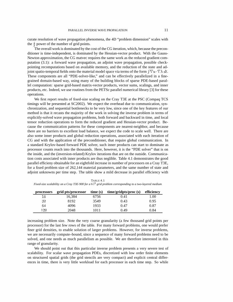
We first report results of fixed-size scaling on the Cray T3E at the PSC (Compaq TCStimings will be presented at SC2002). We expect the overhead due to communication, syn-chronization, and sequential bottlenecks to be very low, since one of the key features of ourmethod is that it recasts the majority of the work in solving the inverse problem in terms ofexplicitly-solved wave propagation problems, both forward and backward in time, and localtensor reduction operations to form the reduced gradient and Hessian-vector product. Be-cause the communication patterns for these components are nearest-neighbor, and becausethere are no barriers to excellent load balance, we expect the code to scale well. There arealso some inner products and global reduction operations, associated with each iteration ofCG and with the application of the preconditioner, that require global communication. Ina standard Krylov-based forward PDE solver, such inner products can start to dominate asprocessor counts reach into the thousands. Here, however, it is the “PDE solver” that is onthe inside, and the (inversion-related) Krylov iterations that are on the outside. Communica-tion costs associated with inner products are thus neglible. Table 4.1 demonstrates the goodparallel efficieny obtainable for an eightfold increase in number of processors on a Cray T3E,for a fixed problem size of 262,144 material parameters, and the same number of state andadjoint unknowns per time step. The table show a mild decrease in parallel efficiency with

TABLE 4.1Fixed-size scalability on a Cray T3E-900 for a653 grid problem corresponding to a two-layered medium

processors grid pts/processor time (s) time/gridpts/proc (s) efficiency16 16,384 6756 0.41 1.0032 8192 3549 0.43 0.9564 4096 1933 0.47 0.87128 2048 1011 0.49 0.84

increasing problem size. Note the very coarse granularity (a few thousand grid points perprocessor) for the last few rows of the table. For many forward problems, one would preferfiner grid densities, to enable solution of larger problems. However, for inverse problems,we are necessarily compute–bound, since a sequence of many forward problems need to besolved, and one needs as much parallelism as possible. We are therefore interested in thisrange of granularity.

We should point out that this particular inverse problem presents a very severe test ofscalability. For scalar wave propagation PDEs, discretized with low order finite elementson structured spatial grids (the grid stencils are very compact) and explicit central differ-ences in time, there is very little workload for each processor in each time step. So while

12 A. AKCELIK, G. BIROS, AND O. GHATTAS

we can express the inverse method in terms of (a moderate number of) forward-like PDEproblems, and while this means we follow the usual “volume computation/surface commu-nication” paradigm, it turns out for this particular inverse problem (involving acoustic wavepropagation), the computation to communication ratio is about as low as it can get for a PDEproblem (and this will be true whether we solve the forward or inverse problem). A non-linear forward problem, vector unknowns per grid point, higher order spatial discretization,unstructured meshes, or an implicit time stepping scheme—all of these would increase thecomputation/communication ratio and produce better efficiencies.

By increasing the number of processors with a fixed grid size, we have studied the effectof communication and load balancing on parallel efficiency in isolation of algorithmic per-formance. We next turn our attention to algorithmic scalability. We characterize the increasein work of our algorithm as problem size increases (mesh size decreases) by the number ofinner (linear) CG and outer (nonlinear) Gauss-Newton iterations. The work per CG iterationinvolves explicit forward and adjoint wave propagation solutions, and their cost scales withthe 4

3power of the number of grid points; a CG iteration also requires the computation of the

integral in (3.3), which is linear in the number of grid points. Ideally, the number of linearand nonlinear iterations would be independent of the problem size; below, we examine thisscalability for both Tikhonov and TV regularization.

Figure 4.1 shows the result of inversion of surface pressure data for a synthetic velocitymodel that describes the geometry of a hemipelvic bone and surrounding volume. Figure 4.1dshows a target surface reconstruction, which was used to generate a piecewise-homogeneous(bone and surrounding medium) 3D material model. Cross sections through this 3D modelare shown for three orthogonal planes, along with the results of the inversion for the finestgrid, which is1293. Solution of the inverse problem at this grid level required 3 hours wallclock time on 128 TCS processors for Tikhonov regularization, and the same amount oftime, but on 256 processors, for TV regularization (the images in the figure correspond toTikhonov regularization). Note that unlike ultrasound imaging, here we are inverting formechanical properties of a medium, not just the geometry of its interface. Note that for thisproblem, with 129 grid points in each direction, we are resolving at best 10 wavelengths ineach direction, which is insufficient to extract fine features of the model. We expect that finergrids will resolve these features in greater detail.

Table 4.2 shows the growth in TV-regularized iterations for the limited memory BFGS(L-BFGS), unpreconditionedGauss-Newton-Krylov (GNK), and preconditionedGauss-Newton-Krylov (PGNK) methods as a function of material model resolution. L-BFGS was not able toconverge for the4913 and35; 937 parameter problems in any reasonable amount of time, andlarger problems weren’t attempted with the method. This is not surprising; limited memorymethods have difficulties with highly ill-conditioned problems. The Gauss-Newton methodsshowed mesh-independence of nonlinear iterations, until the finest grid. Finer grids producegreater heterogeneity and anisotropy of the “material” tensor of the TV regularization term,as can be seen by (3.6). This results in increasing ill-conditioning in the reduced Hessian, andappears to cause the increase in nonlinear iterations (see [16] for a discussion and examplesof this behavior in the context of total variation denoising of images). On the other hand, theinner conjugate gradient iterations appear to be relatively constant per nonlinear iteration forPGNK. To verify that the inner iteration would keep scaling, we ran one nonlinear iteration ona 2573 grid (nearly 17 million inversion parameters) on 2048 TCS processors. This requiredabout 3 hours and 27 CG iterations, which is comparable to the smaller grids. This suggeststhat the preconditioner is very effective.

To verify that the TV term is causing the deterioration in nonlinear iterations, we resolvedthe above problem with Tikhonov regularization for a range of grid sizes from333 to 1293.

PARALLEL INVERSE WAVE PROPAGATION 13

20 40 60 80 100 120

20

40

60

80

100

120

20 40 60 80 100 120

20

40

60

80

100

120

20 40 60 80 100 120

20

40

60

80

100

120

20 40 60 80 100 120

20

40

60

80

100

120

20 40 60 80 100 120

20

40

60

80

100

120

20 40 60 80 100 120

20

40

60

80

100

120

(a)

20 40 60 80 100 120

20

40

60

80

100

120

20 40 60 80 100 120

20

40

60

80

100

120

20 40 60 80 100 120

20

40

60

80

100

120

20 40 60 80 100 120

20

40

60

80

100

120

20 40 60 80 100 120

20

40

60

80

100

120

20 40 60 80 100 120

20

40

60

80

100

120

(b)

20 40 60 80 100 120

20

40

60

80

100

120

20 40 60 80 100 120

20

40

60

80

100

120

20 40 60 80 100 120

20

40

60

80

100

120

20 40 60 80 100 120

20

40

60

80

100

120

20 40 60 80 100 120

20

40

60

80

100

120

20 40 60 80 100 120

20

40

60

80

100

120

(c) (d)

FIG. 4.1. Performance of inversion algorithm on finest grid (1293). Domain sizeL = 100; target velocity

is 20 for bone, 10 for surrounding medium. Total duration is 20.15 � 15 source/receiver arrays on four sides ofthe volume are used; source is a Ricker wavelet with central frequencies of 0.3 (65

3 wave propagation grid) and 0.6(1293 grid). Figure shows cross-sections of inverted and target models. (a) at x=0.25L, 0.5L, 0.75L; (b) at y=0.25L,0.5L, 0.75L; (c) at z=0.25L, 0.5L, 0.75L; and (d) surface model of the target.

14 A. AKCELIK, G. BIROS, AND O. GHATTAS

TABLE 4.2Algorithmic scaling with TV regularization for limited memory BFGS (L-BFGS), unpreconditioned Gauss-

Newton-Krylov (GNK), and Gauss-Newton-Krylov-BFGS (PGNK) methods as a function of material model resolu-tion. For L-BFGS, the number of iterations is reported, and for both L-BFGS solver and preconditioning,m = 200

L-BFGS vectors are stored. For GNK and PGNK, the total number of CG iterations is reported, along with the num-ber of Newton iterations in parentheses. On all material grids up to65

3, the forward and adjoint wave propagationproblems are posed on653 grid� 400 time steps, and inversion is done on 64 TCS processors; for the129

3 materialgrid, the wave equations are on1293 grids� 800 time steps, on 256 processors. In all cases, work per iterationreported is dominated by a reduced gradient (L-BFGS) or reduced-gradient-like (GNK, PGNK) calculation, so thereported iterations can be compared across the different methods. The regularization and TV smoothing parametersare� = 0:004 and" = 0:01. Convergence criterion is10�5 relative norm of the reduced gradient. “*” indicateslack of convergence;y indicates number of iterations extrapolated from converging value after 6 hours of runtime.

grid size material parameters L-BFGS its GNK its PGNK its653 8 16 17 (5) 10 (5)653 27 36 57 (6) 20 (6)653 125 144 131 (7) 33 (6)653 729 156 128 (5) 85 (4)653 4913 * 144 (4) 161 (4)653 35; 937 * 177 (4) 159 (6)653 274; 625 — 350 (7) 197 (6)1293 2; 146; 689 — 1470y (22) 409 (16)

Indeed, the number of nonlinear iterations did not deteriorate with the1293 grid, and thelinear iterations remained constant as well.

These results are encouraging, and demonstrate that the multiscale L-BFGS precondi-tioned Gauss-Newton-Krylov method seems to be scaling reasonably well for such a highlynonlinear and ill-conditioned problem as inverse wave propagation. The increase in nonlineariterations with the TV-regularized Gauss-Newton method at the finest grid suggests a switchto a more robust (but just linearly convergent) Picard iteration [16] far from the optimum,coupled with (Gauss)-Newton once near the region of quadratic convergence. A coarse gridprojection to approximate the compact part of the reduced Hessian, combined with a multi-level solver for the TV component, should help address the mild increase in CG iterations.Overall, we are able to solve a highly nonlinear inverse wave propagation problem with over2 million unknown inversion parameters in just three hours on 256 TCS processors.

REFERENCES

[1] R. Acar and C. R. Vogel,Analysis of bounded variation penalty methods for ill-posed problems, InverseProblems, Vol. 10, p. 1217–1229, 1994.

[2] O. Axelsson,Iterative Solution Methods, Cambridge Press, 1994.[3] S. Balay, K. Buschelman, W.D. Gropp, D. Kaushik, L. Curfman McInnes, B.F. Smith,PETSc Home Page,

http://www.mcs.anl.gov/petsc , 2001.[4] G. Biros and O. Ghattas,Parallel Newton-Krylov-Schur Methods for PDE Constrained Optimization. Part

I: The Krylov-Schur Solver, Technical Report, Laboratory for Mechanics, Algorithm, and Computing,Carnegie Mellon University, 2000.

[5] G. Biros and O. Ghattas,Parallel Newton-Krylov-Schur Methods for PDE Constrained Optimization. Part II:The Lagrange Newton Solver, Technical Report, Laboratory for Mechanics, Algorithm, and Computing,Carnegie Mellon University, 2000.

[6] C. Bunks, F. M. Saleck, S. Zaleski, and G. Chavent,Multiscale Seismic Waveform Inversion, Geophysics, Vol.50, p. 1457-1473, 1995.

[7] G. Chavent and F. Clement,Waveform Inversion Through MBTT Formulation.Technical Report 1839, INRIA,1993.

[8] S.C. Eisenstat and H.F. Walker,Globally Convergent Inexact Newton Methods, SIAM Journal on Optimiza-tion, Vol. 4, No. 2, p. 393–422, 1994.

PARALLEL INVERSE WAVE PROPAGATION 15

[9] A. Griewank,Achieving logarithmic growth of temporal and spatial complexity in reverse automatic differen-tiation, Optimization Methods and Software, Vol.1, p. 35-54, 1992.

[10] J.L. Morales and J. Nocedal,Automatic Preconditioning by Limited Memory Quasi-Newton Updating, SIAMJournal on Optimization, Vol. 10, p. 1079-1096, 2000.

[11] J. Nocedal and S. J. Wright,Numerical Optimization, Springer, 1999.[12] W. W. Symes,Velocity Inversion: A Case Study in Infinite-Dimensional Optimization, Mathematical Program-

ming, Vol. 48 , p. 71-102, 1990.[13] W. W. Symes and J. J. Carazzone,Velocity Inversion by Differential Semblance Optimization, Geophysics,

Vol. 56, No. 5, p. 654-663, 1991.[14] A. Tarantola,Inversion of Seismic Reflection Data in the Acoustic Approximation, Geophysics, Vol. 49, No.

8, p. 1259–1266, 1984.[15] C. R. Vogel,Computational Methods for Inverse Problems, SIAM, Frontiers in Applied Mathematics, 2002.[16] C.R. Vogel and M.E. Oman,Iterative Methods for Total Variation Denoising, SIAM Journal on Scientific

Computing, Vol. 17, p. 227-238, 1996.