OPTIMIZING THE EFFICIENCY OF THE UNITED STATES …schaefer/papers/KongDissertation.pdf · STATES...
260
OPTIMIZING THE EFFICIENCY OF THE UNITED STATES ORGAN ALLOCATION SYSTEM THROUGH REGION REORGANIZATION by Nan Kong BS, Tsinghua University, 1999 MEng, Cornell University, 2000 Submitted to the Graduate Faculty of the School of Engineering in partial fulfillment of the requirements for the degree of Doctor of Philosophy University of Pittsburgh 2006
Transcript of OPTIMIZING THE EFFICIENCY OF THE UNITED STATES …schaefer/papers/KongDissertation.pdf · STATES...
OPTIMIZING THE EFFICIENCY OF THE UNITED
STATES ORGAN ALLOCATION SYSTEM
THROUGH REGION REORGANIZATION
by
Nan Kong
BS, Tsinghua University, 1999
MEng, Cornell University, 2000
Submitted to the Graduate Faculty of
the School of Engineering in partial fulfillment
of the requirements for the degree of
Doctor of Philosophy
University of Pittsburgh
2006

UNIVERSITY OF PITTSBURGH
SCHOOL OF ENGINEERING
This dissertation was presented
by
Nan Kong
It was defended on
November 18th 2005
and approved by
Andrew J. Schaefer, Assistant Professor, Departmental of Industrial Engineering
Brady Hunsaker, Assistant Professor, Department of Industrial Engineering
Prakash Mirchandani, Professor, Katz Graduate School of Business
Jayant Rajgopal, Associate Professor, Department of Industrial Engineering
Mark S. Roberts, Associate Professor, Department of Medicine
Dissertation Advisors: Andrew J. Schaefer, Assistant Professor, Departmental of Industrial
Engineering,
Brady Hunsaker, Assistant Professor, Department of Industrial Engineering
ii
ABSTRACT
OPTIMIZING THE EFFICIENCY OF THE UNITED STATES ORGAN
ALLOCATION SYSTEM THROUGH REGION REORGANIZATION
Nan Kong, PhD
University of Pittsburgh, 2006
Allocating organs for transplantation has been controversial in the United States for decades.
Two main allocation approaches developed in the past are (1) to allocate organs to patients
with higher priority at the same locale; (2) to allocate organs to patients with the greatest
medical need regardless of their locations. To balance these two allocation preferences,
the U.S. organ transplantation and allocation network has lately implemented a three-tier
hierarchical allocation system, dividing the U.S. into 11 regions, composed of 59 Organ
Procurement Organizations (OPOs). At present, a procured organ is offered first at the
local level, and then regionally and nationally. The purpose of allocating organs at the
regional level is to increase the likelihood that a donor-recipient match exists, compared to
the former allocation approach, and to increase the quality of the match, compared to the
latter approach. However, the question of which regional configuration is the most efficient
remains unanswered.
This dissertation develops several integer programming models to find the most efficient
set of regions. Unlike previous efforts, our model addresses efficient region design for the
entire hierarchical system given the existing allocation policy. To measure allocation effi-
ciency, we use the intra-regional transplant cardinality. Two estimates are developed in this
dissertation. One is a population-based estimate; the other is an estimate based on the
situation where there is only one waiting list nationwide. The latter estimate is a refinement
of the former one in that it captures the effect of national-level allocation and heterogeneity
iii
of clinical and demographic characteristics among donors and patients. To model national-
level allocation, we apply a modeling technique similar to spill-and-recapture in the airline
fleet assignment problem. A clinically based simulation model is used in this dissertation
to estimate several necessary parameters in the analytic model and to verify the optimal
regional configuration obtained from the analytic model.
The resulting optimal region design problem is a large-scale set-partitioning problem
in which there are too many columns to handle explicitly. Given this challenge, we adapt
branch and price in this dissertation. We develop a mixed-integer programming pricing
problem that is both theoretically and practically hard to solve. To alleviate this existing
computational difficulty, we apply geographic decomposition to solve many smaller-scale
pricing problems based on pre-specified subsets of OPOs instead of a big pricing problem.
When solving each smaller-scale pricing problem, we also generate multiple “promising”
regions that are not necessarily optimal to the pricing problem. In addition, we attempt to
develop more efficient solutions for the pricing problem by studying alternative formulations
and developing strong valid inequalities.
The computational studies in this dissertation use clinical data and show that (1) regional
reorganization is beneficial; (2) our branch-and-price application is effective in solving the
optimal region design problem.
Keywords: Integer Programming, Branch and Price, Column Generation, Set Partitioning,
Valid Inequality, Organ Transplantation and Allocation, Health Care Resource Alloca-
tion.
iv

TABLE OF CONTENTS
1.0 INTRODUCTION . . . . . . . . . . . . . . . . . . . . . . . . . . . . . . . . . 1
1.1 Current State of Organ Allocation in the U.S. . . . . . . . . . . . . . . . . . 1
1.2 Current Liver Allocation System . . . . . . . . . . . . . . . . . . . . . . . . 5
1.2.1 Membership . . . . . . . . . . . . . . . . . . . . . . . . . . . . . . . . 5
1.2.2 Liver Allocation Process . . . . . . . . . . . . . . . . . . . . . . . . . 6
1.2.3 Problem Statement and Proposed Research Description . . . . . . . . 8
1.3 Contribution . . . . . . . . . . . . . . . . . . . . . . . . . . . . . . . . . . . 13
2.0 LITERATURE REVIEW . . . . . . . . . . . . . . . . . . . . . . . . . . . . . 15
2.1 Previous Research on Organ Transplantation and Allocation . . . . . . . . . 15
2.1.1 Operations Research Literature . . . . . . . . . . . . . . . . . . . . . . 16
2.1.2 Discrete-event Simulation Models . . . . . . . . . . . . . . . . . . . . 18
2.1.3 Medical, Ethical, and Economic Literature . . . . . . . . . . . . . . . 19
2.2 Integer Programming Applications in Health Care . . . . . . . . . . . . . . . 21
2.2.1 Health Care Operations Management . . . . . . . . . . . . . . . . . . 22
2.2.2 Health Care Public Policy and Economic Analysis . . . . . . . . . . . 23
2.2.3 Clinical Applications . . . . . . . . . . . . . . . . . . . . . . . . . . . 24
2.3 Branch and Price . . . . . . . . . . . . . . . . . . . . . . . . . . . . . . . . . 25
3.0 OPTIMIZING INTRA-REGIONAL TRANSPLANTATION THROUGH
EXPLICIT ENUMERATION OF REGIONS . . . . . . . . . . . . . . . . 34
3.1 Introduction . . . . . . . . . . . . . . . . . . . . . . . . . . . . . . . . . . . 34
3.2 A Set-Partitioning Formulation for Region Design . . . . . . . . . . . . . . . 36
3.2.1 A Closed-Form Regional Benefit Estimation . . . . . . . . . . . . . . . 37
v

3.2.2 Data Acquisition and Parameter Estimation . . . . . . . . . . . . . . 40
3.3 An Explicit Enumeration Approach to Region Design Solution . . . . . . . . 42
3.4 Incorporating Geographic Equity . . . . . . . . . . . . . . . . . . . . . . . . 51
3.5 Deficiencies and Further Considerations . . . . . . . . . . . . . . . . . . . . 62
4.0 OPTIMIZING INTRA-REGIONAL TRANSPLANTATION WITH TWO
MODEL REFINEMENTS THROUGH EXPLICIT ENUMERATION
OF REGIONS . . . . . . . . . . . . . . . . . . . . . . . . . . . . . . . . . . . . 64
4.1 Critique of the First Model in Chapter 3 . . . . . . . . . . . . . . . . . . . . 65
4.2 Refined Optimal Region Design Model . . . . . . . . . . . . . . . . . . . . . 67
4.3 Parameter Estimation for the Refined Model . . . . . . . . . . . . . . . . . . 72
4.3.1 Adaptation of a Clinically Based Simulation Model . . . . . . . . . . . 73
4.3.2 Parameter Estimation . . . . . . . . . . . . . . . . . . . . . . . . . . . 74
4.4 Optimizing the Refined Model through Explicit Enumeration of Regions . . 79
4.5 Evaluating the Proposed Regions . . . . . . . . . . . . . . . . . . . . . . . . 86
4.6 National-level Allocation Modeling . . . . . . . . . . . . . . . . . . . . . . . 88
4.6.1 Analogy between Region Design and Fleet Assignment . . . . . . . . . 89
4.6.2 Estimating Spilled Cost and Recaptured Revenue . . . . . . . . . . . 90
4.6.3 Estimating Spill and Recapture Likelihoods with the Simulation . . . 94
4.7 Summary of Assumptions . . . . . . . . . . . . . . . . . . . . . . . . . . . . 95
5.0 A BRANCH-AND-PRICE APPROACH TO OPTIMAL REGION DE-
SIGN SOLUTION . . . . . . . . . . . . . . . . . . . . . . . . . . . . . . . . . 97
5.1 Adaptive Region Generation . . . . . . . . . . . . . . . . . . . . . . . . . . . 98
5.2 A Mixed-Integer Pricing Problem . . . . . . . . . . . . . . . . . . . . . . . . 100
5.3 A Branch-and-Price Algorithmic Framework . . . . . . . . . . . . . . . . . . 106
5.4 Geographic Decomposition . . . . . . . . . . . . . . . . . . . . . . . . . . . 113
5.5 Branching on OPO pairs . . . . . . . . . . . . . . . . . . . . . . . . . . . . . 117
5.6 Implementation and Computational Experiments . . . . . . . . . . . . . . . 119
5.6.1 Introduction to COIN/BCP . . . . . . . . . . . . . . . . . . . . . . . 120
5.6.2 Development of Our Branch-and-Price Application . . . . . . . . . . . 120
5.6.3 Computational Results . . . . . . . . . . . . . . . . . . . . . . . . . . 121
vi

6.0 IMPROVING THE SOLUTION OF THE PRICING PROBLEM . . . 137
6.1 Alternative Formulations . . . . . . . . . . . . . . . . . . . . . . . . . . . . 138
6.2 Polyhedral Study . . . . . . . . . . . . . . . . . . . . . . . . . . . . . . . . . 144
6.2.1 Valid Inequality Class I . . . . . . . . . . . . . . . . . . . . . . . . . . 144
6.2.1.1 Searching the Optimal Set Cardinality in a Special Case . . . 149
6.2.1.2 Cut Generation in the Branch-and-Bound Solution (Class I) . 153
6.2.2 Valid Inequality Class II . . . . . . . . . . . . . . . . . . . . . . . . . 154
6.2.2.1 A Pure Cutting-Plane Algorithm . . . . . . . . . . . . . . . . 159
6.2.2.2 Cut Generation in the Branch-and-Bound Solution (Class II) . 161
6.3 Computational Experiments . . . . . . . . . . . . . . . . . . . . . . . . . . . 163
6.3.1 Alternative Pricing Problem Formulation Comparison . . . . . . . . . 163
6.3.2 Incorporating Valid Inequalities . . . . . . . . . . . . . . . . . . . . . 164
7.0 PROPORTIONAL ALLOCATION GENERALIZATION . . . . . . . . . 168
7.1 Introduction . . . . . . . . . . . . . . . . . . . . . . . . . . . . . . . . . . . 168
7.1.1 Generic Set-Partitioning Formulation . . . . . . . . . . . . . . . . . . 169
7.1.2 Grouping Quantity Generalization . . . . . . . . . . . . . . . . . . . . 169
7.1.3 An Alternative Interpretation of the Generalization . . . . . . . . . . 173
7.1.4 Organ Allocation as an Example . . . . . . . . . . . . . . . . . . . . . 173
7.1.5 1-Commodity Case . . . . . . . . . . . . . . . . . . . . . . . . . . . . 174
7.2 Generalization of the Column Generation Approach . . . . . . . . . . . . . . 175
7.2.1 2-Commodity Grouping Case . . . . . . . . . . . . . . . . . . . . . . . 175
7.2.2 3-Commodity Grouping Case . . . . . . . . . . . . . . . . . . . . . . . 177
7.2.3 K-Commodity Grouping Case . . . . . . . . . . . . . . . . . . . . . . 179
7.3 Generalization of a Class of Valid Inequalities . . . . . . . . . . . . . . . . . 181
8.0 SUMMARY AND FUTURE RESEARCH . . . . . . . . . . . . . . . . . . 188
8.1 Summary . . . . . . . . . . . . . . . . . . . . . . . . . . . . . . . . . . . . . 188
8.2 Future Research . . . . . . . . . . . . . . . . . . . . . . . . . . . . . . . . . 190
8.2.1 Model Refinement and Extension . . . . . . . . . . . . . . . . . . . . 190
8.2.2 Branch-and-Price Solution Improvement . . . . . . . . . . . . . . . . . 193
8.2.3 Generalization . . . . . . . . . . . . . . . . . . . . . . . . . . . . . . . 195
vii
APPENDIX A. APPLICATIONS OF INTEGER PROGRAMMING COL-
UMN GENERATION . . . . . . . . . . . . . . . . . . . . . . . . . . . . . . . 197
APPENDIX B. A LIST OF ORGAN PROCUREMENT ORGANIZATIONS199
APPENDIX C. DETAILED DESCRIPTION OF THE BCP IMPLEMEN-
TATION . . . . . . . . . . . . . . . . . . . . . . . . . . . . . . . . . . . . . . . 202
APPENDIX D. COLUMN GENERATION EFFECT . . . . . . . . . . . . . . 207
APPENDIX E. COLUMN GENERATION EFFECT (CONTD.) . . . . . . 211
APPENDIX F. PRICING PROBLEM SOLUTION OPTION . . . . . . . . 215
APPENDIX G. STRENGTH OF CLASS I VALID INEQUALITY . . . . . 222
APPENDIX H. A SPECIAL CASE OF RPP=(S): UNIMODALITY . . . . 226
BIBLIOGRAPHY . . . . . . . . . . . . . . . . . . . . . . . . . . . . . . . . . . . . 228
viii

LIST OF TABLES
1 U.S. Liver Data between 1996 - 2004 . . . . . . . . . . . . . . . . . . . . . . . 2
2 Effect of Solution Space Reduction . . . . . . . . . . . . . . . . . . . . . . . . 43
3 Connected Subgraph Enumeration . . . . . . . . . . . . . . . . . . . . . . . . 44
4 Description of Data Sets Used in Computational Experiments . . . . . . . . . 45
5 Relative Improvement on Intra-regional Transplant Cardinality . . . . . . . . 45
6 Discrepancy on Intra-regional Transplant Rate with Optimal Configuration . 51
7 The Value of ρc . . . . . . . . . . . . . . . . . . . . . . . . . . . . . . . . . . 53
8 Relative Improvement on the Overall Objective . . . . . . . . . . . . . . . . . 54
9 Reduction of Geographic Inequity when ρ = 103 . . . . . . . . . . . . . . . . 62
10 OPO Service Areas with Population of Less than 9 Million . . . . . . . . . . 65
11 Difference in Clinical and Demographic Characteristics Pertaining to Liver
Transplantation . . . . . . . . . . . . . . . . . . . . . . . . . . . . . . . . . . 66
12 Ratio of the Standard Deviation to the Average of Pure Distribution Likelihood 75
13 Improvement on Intra-regional Transplant Cardinality (max |r| = Maximum
Region Cardinality) . . . . . . . . . . . . . . . . . . . . . . . . . . . . . . . . 80
14 Improvement on Intra-regional Transplant Cardinality (through Explicit Re-
gion Enumeration) . . . . . . . . . . . . . . . . . . . . . . . . . . . . . . . . . 86
15 Paired t Test: Optimal vs. Current (Linear) . . . . . . . . . . . . . . . . . . . 88
16 Paired t Test: Optimal vs. Current (3rd-degree Polynomial) . . . . . . . . . . 89
17 Comparison between the Solutions through Branch and Price and Explicit
Region Enumeration . . . . . . . . . . . . . . . . . . . . . . . . . . . . . . . . 123
18 Improvement on Intra-regional Transplant Cardinality (using Branch and Price)126
ix

19 Paired t Test: Branch and Price vs. Explicit Region Enumeration (Linear) . . 127
20 Paired t Test: Branch and Price vs. Explicit Region Enumeration (Polynomial) 127
21 Region Covers Design Characteristics . . . . . . . . . . . . . . . . . . . . . . 129
22 Initialization Effect (Region Covers Design 20-12-1) . . . . . . . . . . . . . . 130
23 Column Generation Effect (20 covers and each cover with 12 OPOs) . . . . . 132
24 Pricing Problem Solution Options: Design (20,12) . . . . . . . . . . . . . . . 134
25 Rounding Heuristics: (p0 = 0.9) . . . . . . . . . . . . . . . . . . . . . . . . . 135
26 Rounding Heuristics: (p0 = 1.1) . . . . . . . . . . . . . . . . . . . . . . . . . 135
27 Comparison of the Four Equivalent Pricing Problem Formulations . . . . . . 164
28 Strength of Class I Valid Inequalities (RPP 0 0 2) . . . . . . . . . . . . . . . 165
29 Strength of Class I Valid Inequalities (RPP 0 0 10; only consider CPU time) 166
30 Applications of Integer Programming Column Generation . . . . . . . . . . . 198
31 A List of Organ Procurement Organizations . . . . . . . . . . . . . . . . . . . 200
32 A List of Organ Procurement Organizations (Contd.) . . . . . . . . . . . . . 201
33 Column Generation Effect (20 covers and each cover with 14 OPOs) . . . . . 208
34 Column Generation Effect (20 covers and each cover with 10 OPOs) . . . . . 208
35 Column Generation Effect (20 covers and each cover with 8 OPOs) . . . . . 209
36 Column Generation Effect (30 covers and each cover with 10 OPOs) . . . . . 209
37 Column Generation Effect (30 covers and each cover with 8 OPOs) . . . . . 209
38 Column Generation Effect (25 covers and each cover with 12 OPOs) . . . . . 210
39 Column Generation Effect (15 covers and each cover with 12 OPOs) . . . . . 210
40 Pricing Problem Solution Options: Design (20,14) . . . . . . . . . . . . . . . 216
41 Pricing Problem Solution Options: Design (20,10) . . . . . . . . . . . . . . . 217
42 Pricing Problem Solution Options: Design (20,8) . . . . . . . . . . . . . . . . 218
43 Pricing Problem Solution Options: Design (30,10) . . . . . . . . . . . . . . . 219
44 Pricing Problem Solution Options: Design (30,8) . . . . . . . . . . . . . . . . 220
45 Pricing Problem Solution Options: Design (25,12) . . . . . . . . . . . . . . . 220
46 Pricing Problem Solution Options: Design (15,12) . . . . . . . . . . . . . . . 221
47 Strength of Class I Valid Inequalities (RPP 0 0 2) . . . . . . . . . . . . . . . 223
48 Strength of Class I Valid Inequalities (Contd.) (RPP 0 0 2) . . . . . . . . . . 224
x

49 Strength of Class I Valid Inequalities (RPP 0 0 10; only consider CPU time) 225
xi

LIST OF FIGURES
1 Organ Procurement Organization Service Areas . . . . . . . . . . . . . . . . . 5
2 Current Regional Configuration . . . . . . . . . . . . . . . . . . . . . . . . . . 7
3 Current Allocation Policy . . . . . . . . . . . . . . . . . . . . . . . . . . . . . 11
4 Primary non-function (PNF) vs. Cold-ischemia time (CIT) . . . . . . . . . . 41
5 Optimal Regional Configuration (PNF vs. CIT: Linear; The number of regions
is fixed to 11) . . . . . . . . . . . . . . . . . . . . . . . . . . . . . . . . . . . 47
6 Optimal Regional Configuration (PNF vs. CIT: 3rd-degree Polynomial; The
number of regions is fixed to 11) . . . . . . . . . . . . . . . . . . . . . . . . . 48
7 Optimal Regional Configuration (PNF vs. CIT: Linear; The number of regions
is unrestricted) . . . . . . . . . . . . . . . . . . . . . . . . . . . . . . . . . . . 49
8 Optimal Regional Configuration (PNF vs. CIT: 3rd-degree Polynomial; The
number of regions is unrestricted) . . . . . . . . . . . . . . . . . . . . . . . . 50
9 Pareto Frontier – Geographic Equity vs. Allocation Efficiency (PNF vs. CIT:
Linear; The number of regions is fixed to 11) . . . . . . . . . . . . . . . . . . 55
10 Pareto Frontier – Geographic Equity vs. Allocation Efficiency (PNF vs. CIT:
3rd-degree Polynomial; The number of regions is fixed to 11) . . . . . . . . . 56
11 Pareto Frontier – Geographic Equity vs. Allocation Efficiency (PNF vs. CIT:
Linear; The number of regions is unrestricted) . . . . . . . . . . . . . . . . . 57
12 Pareto Frontier – Geographic Equity vs. Allocation Efficiency (PNF vs. CIT:
3rd-degree Polynomial; The number of regions is unrestricted) . . . . . . . . . 58
13 Optimal Configuration vs. Current Configuration (The number of regions is
fixed to 11) . . . . . . . . . . . . . . . . . . . . . . . . . . . . . . . . . . . . . 59
xii

14 Optimal Configuration vs. Current Configuration (The number of regions is
unrestricted) . . . . . . . . . . . . . . . . . . . . . . . . . . . . . . . . . . . . 60
15 Transplant Likelihood Matrix Distance (Simulation vs. Actual Data) . . . . . 76
16 Statistical Analysis for the Rejection Probability Estimation . . . . . . . . . . 77
17 Statistical Analysis for the National Flow Likelihood Estimation . . . . . . . 79
18 Optimal Regional Configuration (PNF vs. CIT: Linear; The maximum regional
cardinality is 7) . . . . . . . . . . . . . . . . . . . . . . . . . . . . . . . . . . 82
19 Optimal Regional Configuration (PNF vs. CIT: 3rd-degree Polynomial; The
maximum regional cardinality is 7) . . . . . . . . . . . . . . . . . . . . . . . . 83
20 Optimal Regional Configuration (PNF vs. CIT: Linear; The maximum regional
cardinality is 8) . . . . . . . . . . . . . . . . . . . . . . . . . . . . . . . . . . 84
21 Optimal Regional Configuration (PNF vs. CIT: 3rd-degree Polynomial; The
maximum regional cardinality is 8) . . . . . . . . . . . . . . . . . . . . . . . . 85
22 Branch-and-Bound Algorithm . . . . . . . . . . . . . . . . . . . . . . . . . . . 107
23 Illustration of Branch and Price . . . . . . . . . . . . . . . . . . . . . . . . . 108
24 Illustration of Geographic Decomposition . . . . . . . . . . . . . . . . . . . . 114
25 Comparison of Branching on Variables and Branching on OPO Pairs . . . . . 119
26 Optimal Regional Configuration Using Branch and Price . . . . . . . . . . . . 125
27 Optimal Regional Configuration Using Branch and Price (Contd.) . . . . . . 126
28 Column Generation Effect (20 covers and each cover with 12 OPOs) . . . . . 133
29 Illustration of Unimodality (l0i = 1000, 500, and 300) . . . . . . . . . . . . . . 167
30 An Illustration of K-tuples Tδ and Ti . . . . . . . . . . . . . . . . . . . . . . 170
31 Illustration of Proportional Allocation in K-grouping . . . . . . . . . . . . . . 171
32 Illustration of a Partial Grouping Process . . . . . . . . . . . . . . . . . . . . 182
33 Column Generation Effect (20 covers and each cover with 14 OPOs) . . . . . 211
34 Column Generation Effect (20 covers and each cover with 10 OPOs) . . . . . 212
35 Column Generation Effect (20 covers and each cover with 8 OPOs) . . . . . . 212
36 Column Generation Effect (30 covers and each cover with 10 OPOs) . . . . . 213
37 Column Generation Effect (30 covers and each cover with 8 OPOs) . . . . . . 213
38 Column Generation Effect (25 covers and each cover with 12 OPOs) . . . . . 214
xiii

39 Column Generation Effect (15 covers and each cover with 12 OPOs) . . . . . 214
40 Illustration of Unimodality (li0 = 200, 100, 50, 30, 20) . . . . . . . . . . . . . . 226
41 Illustration of Unimodality (li0 = 10, 5, 3, 2, 1) . . . . . . . . . . . . . . . . . . 227
xiv

To my wonderful parents, Yang Yi and Kong Qingwen
ACKNOWLEDGMENTS
I would like to express my deepest gratitude to my advisor and mentor, Professor Andrew
Schaefer for directing my dissertation research as well as other studies in so many ways. No
words can describe how thankful to all he has done for me and how lucky I am to be able to
work with him. Without him, I would not be able to accomplish what I have accomplished.
I still vividly remember the first time we met during the new student orientation. Both of us
were new at Pitt. Throughout my five-year PhD studies, he has always been wholeheartedly
supporting me to steer through countless difficulties in all aspects of my life.
I would like to thank my co-advisor and mentor, Professor Brady Hunsaker for supporting
my dissertation research. He has spent an enormous amount of precious time with me
working through many challenges. He has taught me so much that I will benefit from
throughout my career. His intelligence and rigor has influenced me greatly in many ways.
I will cherish forever the time I have spent with both my advisors.
I would also like to thank my committee member, Professor Mark S. Roberts for his
valuable comments and enthusiasm throughout this research. I am also indebted to the
rest of my dissertation committee members, Professors Prakash Mirchandani and Jayant
Rajgopal for their valuable suggestions and insights. I would also like to thank Professor
Mainak Mazumdar for his guidance on my research and career. I truly enjoy our many deep
discussions. He has been a great personal friend of mine.
I am also grateful to my friends in the Computational Optimization Lab who mentally
and emotionally supported me throughout my research. Among them, special thanks to
Oguzhan Alagoz, Zhouyan Wang, Steven Shechter, and Jennifer Kreke for their valuable
insights and comments about my research. Many thanks also go to Mehmet Demirci for his
technical support.
I thank the wonderful staff of the Industrial Engineering Department, Lisa Bopp, Richard
Brown, Minerva Hubbard and Jim Segneff, for providing technical support throughout my
study.
xv

Finally, I am forever indebted to my wonderful parents Yang Yi and Kong Qingwen. I
would have never finished this dissertation without their endless love, encouragement and
unconditional support. I owe them too much!
xvi

1.0 INTRODUCTION
1.1 CURRENT STATE OF ORGAN ALLOCATION IN THE U.S.
According to the National Vital Statistics Report [86], end-stage liver disease (ESLD), i.e.,
chronic liver disease and cirrhosis, is the twelfth leading cause of death in the U.S., accounting
for nearly 30,000 deaths in 2003 alone. Unlike diseases caused by the failure or dysfunction
of some other organs for which patients can resort to alternative therapies, e.g, dialysis
for kidney patients, the only viable therapy for ESLD at present is liver transplantation.
Fortunately, patients at almost any stage of their liver disease receiving a liver transplant
can expect an 80% - 90% five-year survival [129, 197].
Unfortunately, liver transplantation is both costly and limited by the supply of viable
donor organs. The acute hospitalization cost alone has been estimated between $145,000
and $287,000 [83, 120, 179, 189, 192]. More importantly, the increased donation rate has
not kept pace with the demand from patients waiting for transplants (see Table 1). In the
last decade, we have seen the number of patients awaiting transplants doubled from nearly
8,500 at the end of 1996 to more than 17,800 at the end of 2004 whereas there was only a
slight increase regarding the number of yearly procured livers, from 4,522 in 1996 to 6,643.
We use liver transplantation and allocation as the specific example in this research. But
the transplantation and allocation of other types of organs that raises similar issues can also
be addressed using the discussed techniques.
A critical issue regarding liver transplantation and allocation is the efficiency of organ
sharing for cadaveric liver transplants, which constitute the majority of liver transplantation.
Because of poor matching, rejection by transplant centers, or allocation delays resulting in
1
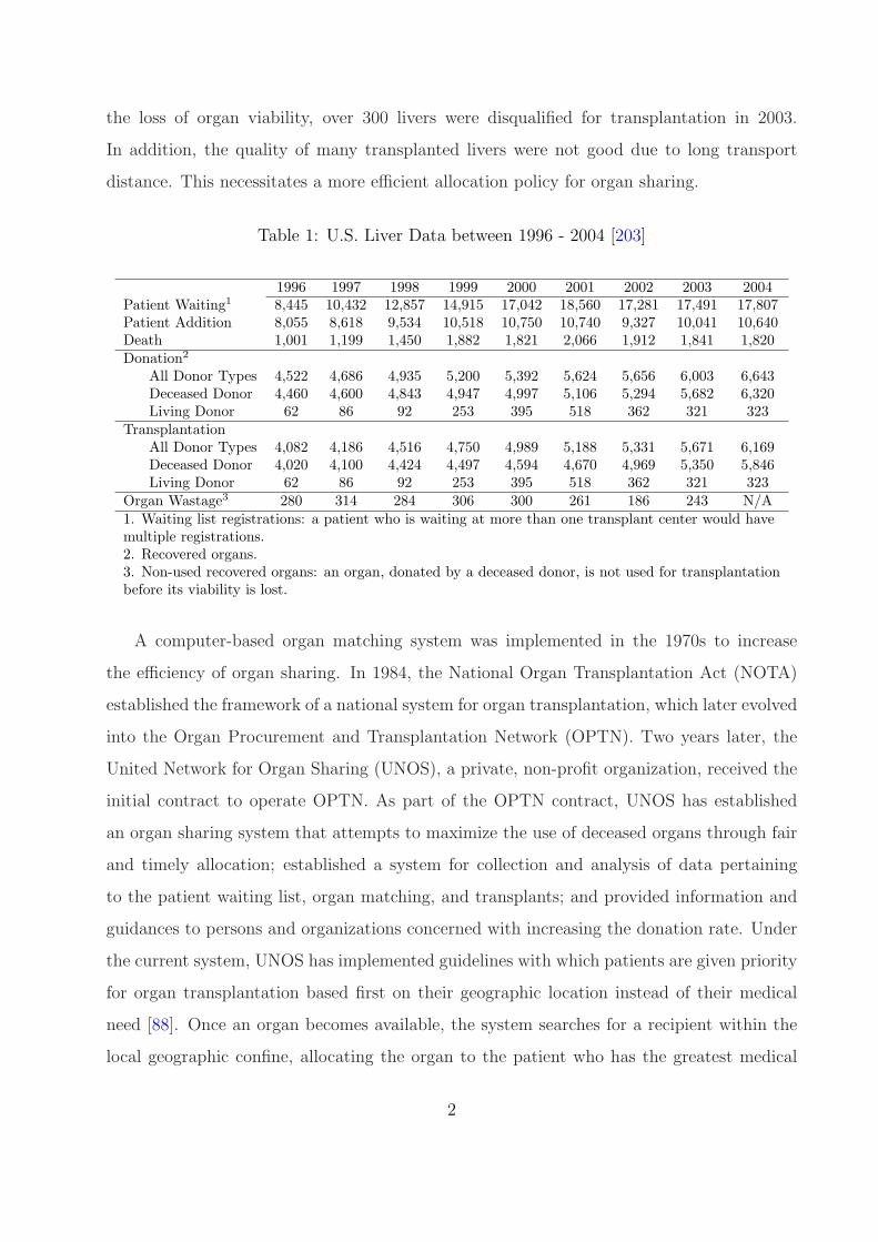
the loss of organ viability, over 300 livers were disqualified for transplantation in 2003.
In addition, the quality of many transplanted livers were not good due to long transport
distance. This necessitates a more efficient allocation policy for organ sharing.
Table 1: U.S. Liver Data between 1996 - 2004 [203]
1996 1997 1998 1999 2000 2001 2002 2003 2004Patient Waiting1 8,445 10,432 12,857 14,915 17,042 18,560 17,281 17,491 17,807Patient Addition 8,055 8,618 9,534 10,518 10,750 10,740 9,327 10,041 10,640Death 1,001 1,199 1,450 1,882 1,821 2,066 1,912 1,841 1,820Donation2
All Donor Types 4,522 4,686 4,935 5,200 5,392 5,624 5,656 6,003 6,643Deceased Donor 4,460 4,600 4,843 4,947 4,997 5,106 5,294 5,682 6,320Living Donor 62 86 92 253 395 518 362 321 323
TransplantationAll Donor Types 4,082 4,186 4,516 4,750 4,989 5,188 5,331 5,671 6,169Deceased Donor 4,020 4,100 4,424 4,497 4,594 4,670 4,969 5,350 5,846Living Donor 62 86 92 253 395 518 362 321 323
Organ Wastage3 280 314 284 306 300 261 186 243 N/A1. Waiting list registrations: a patient who is waiting at more than one transplant center would havemultiple registrations.2. Recovered organs.3. Non-used recovered organs: an organ, donated by a deceased donor, is not used for transplantationbefore its viability is lost.
A computer-based organ matching system was implemented in the 1970s to increase
the efficiency of organ sharing. In 1984, the National Organ Transplantation Act (NOTA)
established the framework of a national system for organ transplantation, which later evolved
into the Organ Procurement and Transplantation Network (OPTN). Two years later, the
United Network for Organ Sharing (UNOS), a private, non-profit organization, received the
initial contract to operate OPTN. As part of the OPTN contract, UNOS has established
an organ sharing system that attempts to maximize the use of deceased organs through fair
and timely allocation; established a system for collection and analysis of data pertaining
to the patient waiting list, organ matching, and transplants; and provided information and
guidances to persons and organizations concerned with increasing the donation rate. Under
the current system, UNOS has implemented guidelines with which patients are given priority
for organ transplantation based first on their geographic location instead of their medical
need [88]. Once an organ becomes available, the system searches for a recipient within the
local geographic confine, allocating the organ to the patient who has the greatest medical
2

need. This organ will normally be sent to other regions only if no one in the original locale
accepts it. This system reflects the medical reality that organs remain viable only for a
limited amount of time prior to the transplants. Organ viability is commonly assessed by
the so-called “cold ischemia time,” i.e., the time interval between when the blood is stopped
to flow to the organ in the donor and when the blood flow is restored in the recipient.
Thus, it is generally not considered desirable to transport an organ of great distance due to
decreased organ viability. However, the most prominent criticism of the current system is
that the desired distribution to patients with greatest medical need has not been achieved
given the ischemic restraints [187].
With the advancement of medical technology, a plausible allocation system is advocated
by taking a more national perspective. Although the present organ preservation technology
does not ensure enough time to establish a true “national list” on which nationwide patients
are given priority truly based on their medical need, some do criticize the system for adhering
to the “local first” allocation policy, arguing that if the size of a local confine increases,
patients with greater need could receive organs without necessarily jeopardizing the organs’
viability. Since the enactment of NOTA, the Department of Health and Human Services
(DHHS) has exercised the federal oversight responsibilities that are assigned to it by NOTA.
In response to concerns expressed about possible inequalities in the existing system of organ
procurement and transplantation, DHHS has created new initiatives and published new
regulations that aim to ensure equity among patients based on medical urgency of patients,
not accidents of geography, in order to adjust the complex national organ allocation system
initiated in the 1970s. For example, on March 16, 2000, DHHS implemented the so-called
“Final Rule” [156], a comprehensive set of guidelines that would affect how organs are
allocated across the country.
Given the shortage of suitable organs, it is not surprising that organ allocation is a
controversial subject. Since the late 1990s a vigorous debate has been going on between the
federal government, which advocates a national system, and states that traditionally suffer
from loss of transplantable organs to other states, such as Louisiana, Wisconsin, Texas,
Arizona, Oklahoma, Tennessee, and South Carolina. These states have either sued the
federal government [204] or introduced legislation [1] in order to restrain the use of organs
3

outside their states. The debate over the organ allocation system became heated after the
publication, legislation, and enactment of the “Final Rule.” It reflects the ideological and
practical divide between the two key players, DHHS, and UNOS and its members, concerning
the procedure and criteria for allocating organs, as well as the procedure for reviewing the
organ allocation system. The root of the disagreement between UNOS and DHHS appears
to be how to address the scarcity of donated organs. Despite the hesitation and criticism
from both sides, a comprise was reached, i.e., the original Final Rule was amended, and
UNOS adopted “larger” geographic areas for allocating livers.
To summarize, the allocation of organs for transplantation is an increasingly contentious
issue in the U.S. and a major concern is allocation efficiency. Both UNOS and DHHS seek
the greatest survival rate for patients and the greatest utilization rate for organs used in
transplantation. Both of them try to increase organ donation, and attempt to limit costs to
health care providers and patients. However, their objectives may become quite disparate
at the operational level to which all above objectives are mutually related.
For liver allocation, the concern of allocation efficiency is based on the fact that the
advancement of organ preservation technology only partially supports the argument of people
who advocate the “national list.” The medically acceptable cold ischemia time (CIT) for
livers is 12 - 18 hours [158], which provides livers with the opportunity of being offered
nationally, in contrast with hearts or lungs, which must be transplanted immediately. On
the other hand, compared with kidneys whose medically acceptable cold ischemia time is
24 hours, a single “national list” certainly cannot guarantee the viability of donated livers.
A compromise between liver sharing locally and nationally is desired and reflected in the
current UNOS liver allocation system.
4

1.2 CURRENT LIVER ALLOCATION SYSTEM
1.2.1 Membership
Currently, every transplant hospital program, organ procurement organization, and histo-
compatibility laboratory in the U.S. is a UNOS member. Other UNOS members include:
voluntary health organizations, general public members, and medical professional and sci-
entific organizations. As of July, 2004, UNOS included 412 total members as follows: 258
transplant centers, 3 consortium members, 59 organ procurement organizations, 154 histo-
compatibility laboratories, 8 voluntary health organizations, 11 general public members, and
25 medical professional/scientific organizations [88] (note that several members are double
counted).
Figure 1: Organ Procurement Organization Service Areas as in 1997 [158]
Among these members, organ procurement organizations (OPOs) are the key component
in the allocation system, the following discussion thus focuses on their operation in the organ
allocation process (see Figure 1). OPOs are non-profit independent organizations authorized
by the federal government that serve as the vital link between the donor and recipient. The
current arrangement of 59 OPOs nationwide evolved gradually, reflecting improvements in
transplantation science, organ preservation, and other factors. Unlike early days when the
donor and recipient were often in the same building, OPOs attempt to match patients with
5

donated organs even if the procurement and transplant occur far apart geographically. Each
OPO is responsible for identifying donors and retrieving organs for transplantation in a
designated geographic area. The designated geographic area served by an OPO ranges in
size from part of a state, to a entire state, to multi-state areas covering part or all of several
states. OPOs are also in charge of preservation and distribution of organs for transplantation
within a reasonable time frame, as well as encouraging donation.
1.2.2 Liver Allocation Process
Once an organ of any kind is procured by an OPO, a complex allocation process starts with
the OPO seeking a recipient within the local area served by the OPO and then outside the
area. A sequence of matching efforts are made according to the current allocation policy
and based on medical and other criteria such as blood type, tissue type, size of the organ,
medical urgency of the patient, as well as time already spent on the waiting list, and distance
between the donor and patient. A computer program designed by UNOS ranks a list of
potential recipients with respect to medical urgency status and informs the procuring OPOs
accordingly. Each type of organ has a specific matching algorithm because of the difference
among organs in their cold ischemia time and donor-recipient compatibility requirements.
After obtaining the list of potential recipients, or candidates, the transplant coordinator
contacts the transplant surgeon caring for the top-ranked patient to offer the organ. If the
surgeon or the transplant center that conducts the transplant surgery declines the organ for
some clinical reasons or other considerations, then the surgeon caring for the next patient on
the list is contacted. Once the organ is accepted, its transportation arrangements are made
and the surgery is scheduled.
For livers, the list of candidates includes three segments: the local (or OPO), the regional,
and the national levels. To be specific, (1) at the local level, all matched “local” patients in
rank order by their medical urgency status; (2) at the regional level, all matched patients
outside the local area but within the area’s OPTN region in similar rank order; (3) at
the national level, all matched patients outside the region in rank order. This reflects the
three-tier hierarchy of the current liver allocation system introduced by UNOS that was
6

intended to facilitate organ sharing. At the regional level, the second tier of the hierarchy
in the organ allocation system, organs are matched with patients from other OPOs within
the same OPTN region. Intuitively, if the region is large, more organ-recipient matches are
likely to exist. However, an organ more likely needs to travel to a recipient OPO that is
far apart from the donor OPO. As a result, a longer cold ischemia time would occur and
the organ quality would further decay. On the other hand, if the region is small, the organ
quality is likely to be high since an organ is less likely to need to travel to a distant recipient
OPO. However, the recipient pool is small, and thus it may be less likely to find a donor-
recipient match. Therefore, the hierarchical system indicates the trade-off between organ
utilization and organ quality decay. Currently, the national UNOS membership is divided
into 11 geographic regions (see Figure 2).
Figure 2: Current Region Map [88]
Under the current UNOS allocation policy, adult patients are classified into groups ac-
cording to a point system designed by UNOS assessing medical urgency status. A simplified
classification of adult patients includes two groups: “Status 1” patients and “MELD” pa-
tients. Status 1 patients are defined to have fulminant liver failure with a life expectancy of
less than seven days [158]. They are assigned points based on their blood type compatibility
with the cadaveric liver and their waiting time. Two subgroups of Status 1 patients are
Status 1A and Status 1B. All other adult patients are assigned a “MELD” (Model for End-
7
Stage Liver Disease) score. MELD scores are integers ranging from 6 to 40, where higher
scores indicate more serious illness. MELD patients are ranked lexicographically by MELD
score, then blood type compatibility, and finally waiting time.
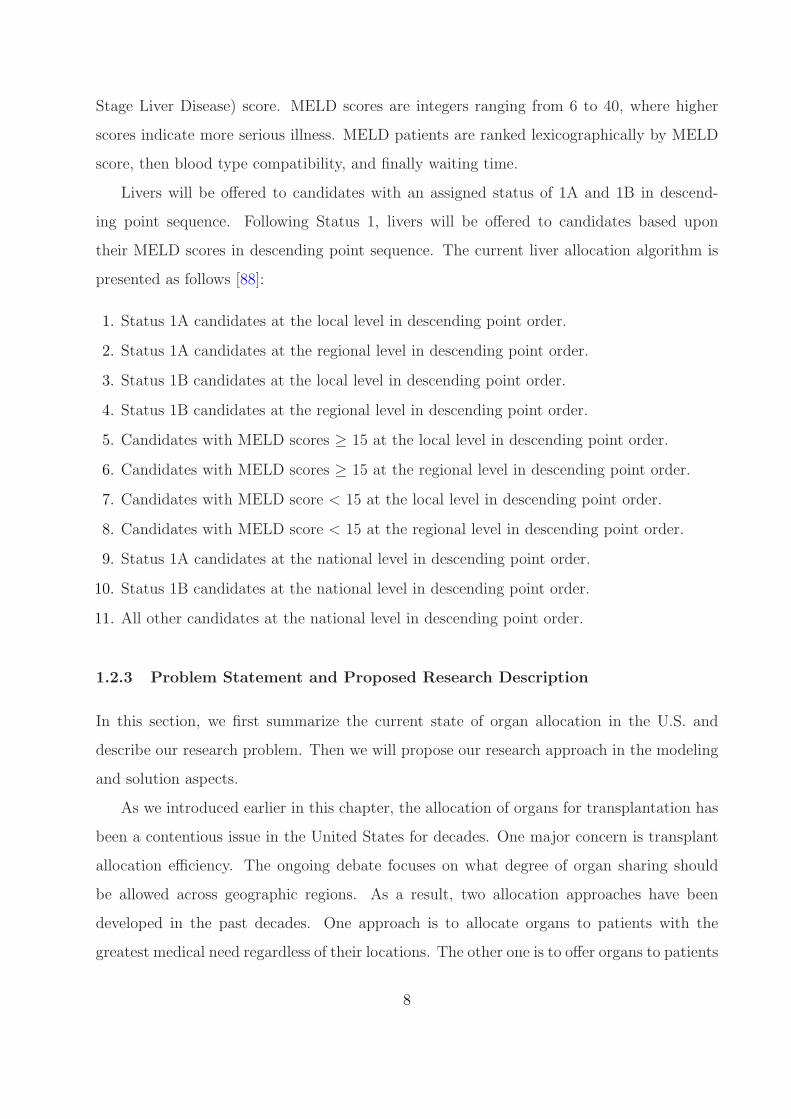
Livers will be offered to candidates with an assigned status of 1A and 1B in descend-
ing point sequence. Following Status 1, livers will be offered to candidates based upon
their MELD scores in descending point sequence. The current liver allocation algorithm is
presented as follows [88]:
1. Status 1A candidates at the local level in descending point order.
2. Status 1A candidates at the regional level in descending point order.
3. Status 1B candidates at the local level in descending point order.
4. Status 1B candidates at the regional level in descending point order.
5. Candidates with MELD scores ≥ 15 at the local level in descending point order.
6. Candidates with MELD scores ≥ 15 at the regional level in descending point order.
7. Candidates with MELD score < 15 at the local level in descending point order.
8. Candidates with MELD score < 15 at the regional level in descending point order.
9. Status 1A candidates at the national level in descending point order.
10. Status 1B candidates at the national level in descending point order.
11. All other candidates at the national level in descending point order.
1.2.3 Problem Statement and Proposed Research Description
In this section, we first summarize the current state of organ allocation in the U.S. and
describe our research problem. Then we will propose our research approach in the modeling
and solution aspects.
As we introduced earlier in this chapter, the allocation of organs for transplantation has
been a contentious issue in the United States for decades. One major concern is transplant
allocation efficiency. The ongoing debate focuses on what degree of organ sharing should
be allowed across geographic regions. As a result, two allocation approaches have been
developed in the past decades. One approach is to allocate organs to patients with the
greatest medical need regardless of their locations. The other one is to offer organs to patients
8
with higher priority at the same locale. There are biological reasons for using organs locally:
transplantable organs are perishable resources. Cold ischemia time reduces organ viability
and thus transplant success rate. To balance the two allocation approaches, UNOS uses
a three-tier hierarchical allocation system, dividing the U.S. into 11 regions, composed of
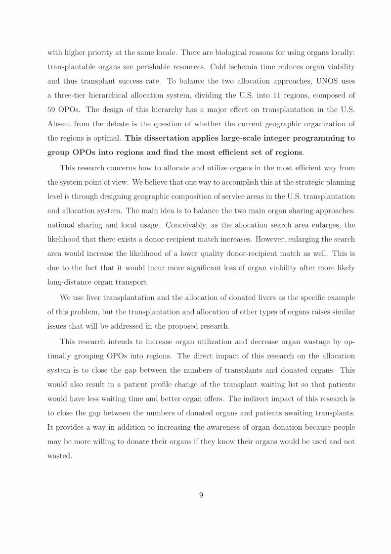
59 OPOs. The design of this hierarchy has a major effect on transplantation in the U.S.
Absent from the debate is the question of whether the current geographic organization of
the regions is optimal. This dissertation applies large-scale integer programming to
group OPOs into regions and find the most efficient set of regions.
This research concerns how to allocate and utilize organs in the most efficient way from
the system point of view. We believe that one way to accomplish this at the strategic planning
level is through designing geographic composition of service areas in the U.S. transplantation
and allocation system. The main idea is to balance the two main organ sharing approaches:
national sharing and local usage. Conceivably, as the allocation search area enlarges, the
likelihood that there exists a donor-recipient match increases. However, enlarging the search
area would increase the likelihood of a lower quality donor-recipient match as well. This is
due to the fact that it would incur more significant loss of organ viability after more likely
long-distance organ transport.
We use liver transplantation and the allocation of donated livers as the specific example
of this problem, but the transplantation and allocation of other types of organs raises similar
issues that will be addressed in the proposed research.
This research intends to increase organ utilization and decrease organ wastage by op-
timally grouping OPOs into regions. The direct impact of this research on the allocation
system is to close the gap between the numbers of transplants and donated organs. This
would also result in a patient profile change of the transplant waiting list so that patients
would have less waiting time and better organ offers. The indirect impact of this research is
to close the gap between the numbers of donated organs and patients awaiting transplants.
It provides a way in addition to increasing the awareness of organ donation because people
may be more willing to donate their organs if they know their organs would be used and not
wasted.
9

In this research, we present an integer programming modeling framework. Each decision
variable in the resulting integer programming models indicates whether the corresponding
potential region is chosen in the optimal set of regions. Our objective is to design a regional
configuration such that some outcome associated with allocation efficiency and/or equity
is maximized. We only address efficiency in the first model. As a result, the model is a
set-partitioning model with constraints restricting each OPO to be contained in exactly one
region in the optimal regional configuration. In the second model, we address both allocation
efficiency and geographic equity. Consequently, the model is a two-objective combinatorial
optimization problem with set-partitioning constraints as in the first model and one decision
variable modeling geographic equity. This dissertation focuses on the first model.
In our research, we need to estimate a specified outcome for each potential region regard-
ing allocation efficiency. Given a potential region, this specified outcome is the number of
transplants at the regional level where the organs are procured within the potential region.
Consequently, the outcome associated with geographic equity considered in this research is
defined as the likelihood that a transplant at the regional level would be received by a pa-
tient from a recipient OPO. Note that the integer programming framework presented in this
research is applicable to the region design problem considering many other system outcomes.
We simplify the current allocation policy by grouping Status 1A and Status 1B patients
as Status 1 patients and grouping all MELD patients together. This simplification can be
justified by the fact that the major difference among patients in terms of medical urgency
is between Status 1 patients and MELD patients. It should be noted that this simplified
version still maintains the three-tier hierarchy. The resulting six-phase allocation algorithm
is as follows and is shown in Figure 3.
Phase 1 Status 1 patients within the procuring OPO.
Phase 2 Status 1 patients within the procuring region.
Phase 3 MELD patients within the procuring OPO.
Phase 4 MELD patients within the procuring region.
Phase 5 Status 1 patients nationally.
Phase 6 MELD patients nationally.
10

Regional
National
Stat
us 1
MEL
D
Local (OPO)
1
2
3
4
5
6
Figure 3: Current Allocation Policy
The core of estimating this outcome is to estimate the likelihood that a candidate from
a recipient OPO would accept an organ from a donor OPO. To estimate the likelihood with
the societal perspective, we consider patients at each step of the allocation process as a whole
and introduce the notion of proportional allocation that simplifies the dynamic nature of the
system. In other words, we consider the measure of this outcome during a long run and in
the expected sense. Therefore, within the above simplified allocation policy, we do not rank
patients in descending point order at each phase of the allocation algorithm.
We develop two analytic estimates. In the first estimate, which is presented in Stahl et
al. [195], we use patient population to estimate the likelihood. In the second estimate, we
make two refinements to incorporate the national-level allocation impact on region design
and heterogeneity in donors’ and patients’ clinical and demographic characteristics. Since
the effect of national-level allocation depends on the regional configuration, it is impossible to
measure this effect in reality where the regional configuration is fixed. We adapt a clinically
based simulation model, LASM [188], that simulates the allocation process with real clinical
11
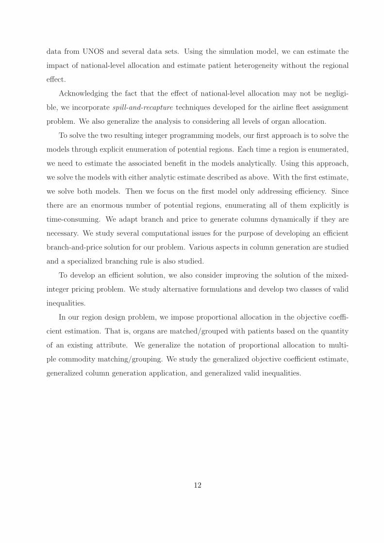
data from UNOS and several data sets. Using the simulation model, we can estimate the
impact of national-level allocation and estimate patient heterogeneity without the regional
effect.
Acknowledging the fact that the effect of national-level allocation may not be negligi-
ble, we incorporate spill-and-recapture techniques developed for the airline fleet assignment
problem. We also generalize the analysis to considering all levels of organ allocation.
To solve the two resulting integer programming models, our first approach is to solve the
models through explicit enumeration of potential regions. Each time a region is enumerated,
we need to estimate the associated benefit in the models analytically. Using this approach,
we solve the models with either analytic estimate described as above. With the first estimate,
we solve both models. Then we focus on the first model only addressing efficiency. Since
there are an enormous number of potential regions, enumerating all of them explicitly is
time-consuming. We adapt branch and price to generate columns dynamically if they are
necessary. We study several computational issues for the purpose of developing an efficient
branch-and-price solution for our problem. Various aspects in column generation are studied
and a specialized branching rule is also studied.
To develop an efficient solution, we also consider improving the solution of the mixed-
integer pricing problem. We study alternative formulations and develop two classes of valid
inequalities.
In our region design problem, we impose proportional allocation in the objective coeffi-
cient estimation. That is, organs are matched/grouped with patients based on the quantity
of an existing attribute. We generalize the notation of proportional allocation to multi-
ple commodity matching/grouping. We study the generalized objective coefficient estimate,
generalized column generation application, and generalized valid inequalities.
12

1.3 CONTRIBUTION
To the best of our knowledge, this research is the first one that considers facilitating organ
transplantation and allocation through optimally organizing geographic transplantation and
allocation service areas in the three-tier hierarchical allocation system. In this research, we
optimize the entire hierarchical system with the existing allocation policy.
In this dissertation, two major contributions are as follows. To design the optimal regional
configuration, we develop a modeling framework that, we believe, can assist policy makers in
refining the hierarchical system to facilitate organ sharing. To solve the resulting large-scale
integer program, we adapt branch and price. Our solution development provides insight into
algorithmic and computational issues regarding branch-and-price algorithms. It also shows
the potential of branch-and-price application in large-scale and complex health care delivery
systems.
The remainder of this dissertation is organized as follows: Chapter 2 first describes
many studies of organ transplantation and allocation in various aspects with emphasis on
operations research applications and simulation models, and the previous work related to
allocation region design. Chapter 2 then addresses some integer programming applications
in health care systems optimization and medical decision making. Chapter 2 also discusses
the literature related to column generation, and branch and price. Chapter 3 formulates
the integer programming models and presents the first objective coefficient estimate based
on patient population. Chapter 3 also discusses the solution of both models through ex-
plicit enumeration of regions. Chapter 4 refines the first objective coefficient estimate with
incorporation of the effect of national-level allocation and heterogeneity in patients’ clinical
and demographic characteristics. Chapter 4 also describes our adaptation of the simulation
model, estimation of parameters required in the analytic estimate, and validation of the
solution using the simulation model. Chapter 5 presents the branch-and-price application to
the regional design problem and discusses several inherent computational issues. Chapter 6
presents a few approaches to improve the pricing problem solution in the branch-and-price
application. Chapter 7 considers a generalization of the proportional allocation scheme in
13

several aspects including the objective coefficient estimation, the pricing problem construc-
tion, and the pricing problem solution improvement. Chapter 8 summarizes the conclusions
drawn in the previous chapters and gives possible future research directions.
14
2.0 LITERATURE REVIEW
In this chapter, we review the literature related to our study. In Section 2.1, we survey
studies regarding organ transplantation and allocation in various fields. The emphasis of
this section is those studies closely related to operations research. In Section 2.2, we describe
some integer programming applications to decision making in health care system planning
and management. In Section 2.3, we first briefly introduce branch and price with an emphasis
on column generation. We then summarize some computational considerations in branch and
price, particularly in column generation. We also list some applications of branch and price
(and more generally, integer programming column generation).
2.1 PREVIOUS RESEARCH ON ORGAN TRANSPLANTATION AND
ALLOCATION
In this section, we review previous work dealing with various issues arising in organ trans-
plantation and allocation. Due to its importance, organ transplantation and allocation has
drawn attention from a wide spectrum of research fields. In Section 2.1.1 we describe many
studies in the operations research literature that use a variety of OR tools to address many
problems with various scales and at different levels of the allocation system. In Section
2.1.2 we describe several simulation models of the liver allocation system and discuss their
contributions in developing organ allocation policies. In Section 2.1.3 we survey a number
of studies regarding medical, ethical, and economical issues related to organ transplantation
and allocation. We do not intend to present an exhaustive list here. Our objective is rather
to emphasize the vast research interest on organ transplantation and allocation.
15
2.1.1 Operations Research Literature
The application of operations research techniques to problems arising in organ transplanta-
tion and allocation started in the 1980s. The operations research literature includes several
studies that address various aspects of organ transplantation and allocation. In the last two
decades, the majority of the studies address donor-recipient matching for transplantation
to optimize some kind of conceptual matching reward or existing quantifiable metric. The
focus of these studies can be classified into two categories: those that consider the potential
recipient’s perspective in accepting or rejecting an organ offer, and those that consider the
centralized decision maker’s perspective, seeking global optimal strategies of allocating mul-
tiple organs to a set of candidates. For a comprehensive literature review of O.R. applications
in organ transplantation and allocation, we refer to Alagoz et al. [10].
One of the first papers modeling the recipient’s perspective is David and Yechiali [58],
who considered when a patient should accept or reject a liver for transplant. The authors first
assumed that organs arrive at fixed time intervals and provided a time-dependent control-
limit optimal policy. They then considered the case where the organ arrival is a renewal
process and assumed that patient health is always deteriorating. One shortcoming in this
paper is that the authors did not consider the actual matching criteria. In more recent stud-
ies that combined analytical and empirical research, Ahn and Hornberger [5] and Hornberger
and Ahn [111] developed a Markov decision process (MDP) model to design kidney accep-
tance policies for potential recipients that explicitly incorporate patient preference. They
demonstrated that some patients can afford to be selective when making transplant decisions.
Most recently, Alagoz et al. [7] developed a MDP model to design optimal control-limit liver
acceptance policies for living-donor transplantation based on abundant clinical data. The
empirical study in [9] applied the MELD scoring system and laboratory values to estimate
the progression of ESLD. Similar MDP models were developed in Alagoz [6] and Alagoz
et al. [8] to address the transplant timing issue for cadaveric donors. The former model
considers a waiting list whose full description is assumed to be available, whereas the latter
one considers an implicit waiting list. For an introduction to MDPs, we refer to Puterman
[168].
16

Most of the previous work modeling the centralized decision marker’s perspective consid-
ers multiple recipient candidates and organ offers given the stochastic nature of their arrivals
and status. Compared to the above single candidate case, this case treats many candidates
competing for the offers. It is more desirable and brings the analysis closer to reality. Righter
[176] formulated the problem as a stochastic sequential assignment problem [64] and devel-
oped properties of the optimal policy. David and Yechiali [59] studied one version of the
problem in infinite horizon and with simultaneous arrivals of candidates and offers. David
and Yechiali [60] considered another version of the problem where the offers arrive randomly.
They studied several cases with various assumptions on the problem parameters and derived
optimal matching policies that maximize the total (discount) reward.
It is well known that the conflict between efficiency and equity is at the root of the
allocation system and a trade-off has to be made due to the scarcity of organ supply. To
gain a better understanding of this trade-off, several researchers have attempted to address
it empirically or analytically. Zenios et al. [224] developed a Monte Carlo simulation model
to compare four alternative kidney allocation policies, accommodating the dynamics of re-
cipient and donor characteristics, patient and graft survival rates, and the quality of life.
The model simulated the operations of a single OPO and attempted to predict the evolution
of the waiting list in 10 years. The authors concluded that evidence-based organ allocation
strategies in cadaveric kidney transplantation would yield improved efficiency and equity
measures compared with the point system currently utilized by UNOS. However, the au-
thors limited the matching in the service area of a single OPO. Clearly the impact of organ
distribution to other OPOs and organ supply from other OPOs is not negligible, especially
in the currently existing liver allocation system. Zenios et al. [223] considered the kidney
allocation system more analytically. They used a fluid model to represent the organ alloca-
tion problem and formulated an objective function that captures both efficiency and equity
criteria. To maximize the objective, they developed a heuristic dynamic index policy. The
authors also used a simulation model to compare the developed policies with the existing
policy.
More recently, Su and Zenios [198] considered the cases where candidates do and do not
have autonomy — the right to refuse a kidney in anticipation of a superior future kidney.
17

For the case where candidates are non-autonomous, they represented the kidney allocation
problem as a sequential stochastic assignment problem. Each candidate is of his own type
that is determined with a snapshot of the waiting list. Kidney types are random and revealed
upon arrival. The reward from allocating a kidney to a particular candidate depends on both
their types. The objective is to allocate kidneys to candidates so that the total expected
reward is maximized. The authors focused on partition policies in which the spaces of
kidney and candidate types are divided into domains and a subset of kidneys in a particular
kidney domain is assigned with a subset of candidates in a matched candidate domain. The
authors also showed that the optimal partition policy performs poorly when candidates are
autonomous. Numerical studies were presented for both cases. There are several unrealistic
aspects in their model: first, the authors assumed that the number of kidneys are the same as
that of candidates, although it is well known that available transplantable organs are scarce
goods. Second, the authors in their model did not incorporate patient ranking in the waiting
list, which has been a basic criterion in the current UNOS matching algorithm. Third,
the authors derived an incentive compatibility condition to model candidate autonomy and
verified it indirectly by only checking the implications of the condition on partition policies,
obtained from the cases where candidate autonomy is not allowed. Unfortunately, this
condition may not actually be satisfied by most transplant candidates.
2.1.2 Discrete-event Simulation Models
Several researchers have attempted to clarify the existing issues in the organ transplantation
and allocation system by developing discrete-event simulation models that compare different
allocation policies. UNOS and Pritsker Corporation developed the UNOS Liver Allocation
Model (ULAM) that considers the patient listing process, organ availability, and UNOS
matching criteria [166, 167]. The primal goal of the model is to evaluate the effects of
creating a national waiting list. The CONSAD Research Corporation developed a simulation
model that assumes all patients are registered in the national waiting list [172]. The model
considers the progression of patient liver disease, including possible death while awaiting
transplants. It allows policy makers to project the impact of relevant important issues on
18

organ donation, organ allocation policy, geographic distribution of organs, and transplant
center proficiency. Recently, Shechter et al. [188] developed a clinically based discrete-event
simulation model, the Liver Allocation Simulation Model (LASM), to provide insight into
the effects of various organ allocation schemes on outcomes in liver transplantation. This
simulation was also intended to capture the regional effect in organ allocation by modeling
the currently effective UNOS liver matching algorithm and comparing outcomes with respect
to various potential regional configurations.
2.1.3 Medical, Ethical, and Economic Literature
Liver allocation is a complex process in which many factors may influence the outcomes
of transplants in different aspects. Along with transplantation technology advances, many
medical researchers have put enormous effort in detecting and understanding these factors
and in controlling them to increase organ allocation efficiency. These efforts provided guid-
ance for development and improvement of the current liver allocation system. We shall first
survey the literature on the effects of several factors, including donor-recipient blood type
similarity, cold ischemia time, and others.
It is evident that blood type matching plays a central role in the current UNOS allocation
system. Gordon et al. [102] reviewed liver allografts in 520 patients to determine the effect of
donor-recipient mismatch or incompatibility between different blood groups on graft survival.
They recommended that nonidentical or incompatible grafts be limited to some groups of
patients. English et al. [81] found that potential group O recipients waited significantly
longer than other groups for transplantation. AB, the group with the shortest waiting time,
however, was receiving mismatched grafts with the highest probability. de Meester et al. [61]
studied various blood type matching policies for highly urgent liver patients to determine the
effect of donor-recipient mismatch and showed that a restricted ABO-compatible matching
policy described those patients the highest probability of acquiring a liver transplant in
the Eurotransplant liver program. Bjoro et al. [30] observed that patients receiving ABO-
identical donor livers had significantly higher patient survival rates compared with those
receiving ABO-compatible donor livers.
19
Much of the debate on allocation preference indicates that cold-ischemia time and graft
transport distance are critical to outcomes in liver transplantation. With a logistic regression
model, Furukawa et al. [92] observed that the retransplantation rate and primary nonfunc-
tion rate rose significantly as the cold-ischemia time increased. Stahl et al. [196] drew a
similar conclusion through a meta-analytic review. Researchers have attempted to develop
new solutions to extend medically acceptable cold ischemia time. Adam et al. [3] studied the
use of the UW solution in liver transplantation. Their findings suggested that cold-ischemia
time in the UW solution for longer than 12 hours is a risk factor for graft function and patient
survival. Piratvisuth et al. [162] and Totsuka et al. [200] concluded that cold-ischemia time
is an important determinant of outcomes after liver transplantation. Totsuka et al. [200]
further recommended that long-distance graft transportation be avoided.
Nair et al. [152] and Yoo and Thuluvath [220] studied the impact of race and socioeco-
nomic status on liver transplantation. They reported that race is an independent predictor
of short- and long-term survival after liver transplantation. They also showed that socioeco-
nomic status (e.g., income, education, and insurance) may be associated with survival. The
empirical studies with respect to donor factors include Oh et al. [157] on donor age, Zeier
et al. [222] on donor gender, Zipfel et al. [225] on donor health status, and Yasutomi et al.
[219] on the size of donor livers.
As alluded earlier, not different from the allocation system of any scarce and/or expen-
sive health resource, conflicting issues, such as efficiency and equity, emerge in the liver
allocation system. Empirical evidence appeared in Rosen et al. [178] who observed that
liver transplant survival rates fell with advancing levels of urgency, resulting in a conflict
between efficiency and equity in organ allocation. Medical researchers, particularly health
economists, are interested in prioritizing these issues in the system. It is both an ethical
dilemma [36] and an economic dilemma [15]. Ubel and Loewenstein [201, 202] surveyed pub-
lic attitudes toward the trade-off between efficiency and equity. Koch [123, 126] provided
a comprehensive discussion on the ethical and economic considerations regarding organ al-
location and transplantation in the current system. The same author stated a preliminary
attempt to resolve the dilemma at the national level by the use of Geographic Information
System (GIS) tools [124]. In the paper, the author emphasized one factor that affects the
20

outcomes, the loss of organ viability. He sought better routing for the distribution of organs,
especially organs procured from remote areas. All his arguments are summarized in [125].
2.2 INTEGER PROGRAMMING APPLICATIONS IN HEALTH CARE
This section describes a few integer programming applications in health care. It is not meant
to be an inclusive survey but rather to bring attention to integer programming applications
in many areas in health care. Operations research techniques, tools, and theories have long
been applied to a wide range of issues and problems in health care. Brandeau et al. [35]
offered a vast collection of OR applications in health care, with particular emphasis on health
care delivery. This section will largely follow the perspective and treatment presented in [35]
on OR applications in health care.
In both rich and poor nations, public resources for health care are inadequate to meet
demand. Policy makers and health care providers must determine how to provide the most
effective health care to citizens using the limited resources that are available. Therefore,
policy makers need effective methods for planning, prioritization, and decision making, as
well as effective methods for management and improvement of health care systems [35]. The
planning and management decisions faced by health care policy makers are grouped into two
broad areas: health care planning and organizing, and health care delivery. The goals of
decision making in these two areas are the same although the problems arising in the two
areas may be of different natures. Good planning and organizing today is for good delivery
tomorrow. Three main areas of applications are: (1) health care operations management,
(2) public policy and economic analysis, and (3) clinical applications.
Integer programming has been well known for its application to planning, organizing, and
delivery. It has also been well known for its application to management and improvement
of systems in various sectors. This is no exception in the health care domain. Integer
programming applications can be found in all three application areas listed above.
21

2.2.1 Health Care Operations Management
In health care operations management, the majority of work has been done in locating health
care facilities. Daskin and Dean [55] reviewed various models for health care facility location
and surveyed their applications in various problems. There has been a great deal of research
on basic location models including the set covering model, the maximal covering model,
and the p-median model [54, 91, 103, 142]. The extensions of these three basic models plus
two others (the p-center problem and the uncapacitated fixed charge model) in health care
location research can be classified into three categories: accessibility models, adaptability
models, and availability models [55].
Accessibility means the ability of patients or clients to reach the health care facility, or
in some cases, the ability of the health care providers to reach patients. Accessibility models
normally tend to take a snapshot of the system and plan for those conditions. As such, they
are static models. For example, Eaton et al. [76] used the maximal covering model to assist
planners in selecting permanent bases for their emergency medical service. Jacobs et al. [115]
used a capacitated p-median model to optimize collection, testing and distribution of blood
products in Virginia and North Carolina. Other applications include Mehrez et al. [148]
and Sinuany-Stern et al. [190] for locating hospitals, McAleer and Naqvi [147] for relocating
ambulance, and Price and Turcotte [165] for locating a blood donor clinic. Adaptability
models are those considering future uncertainty on the conditions under which a system will
operate. As such, they tend to take a long-term view of the system. Carson and Batta
[41] considered the problem of locating an ambulance on university campus in response to
changing daily conditions. ReVelle et al. [173] proposed a number of variants of a conditional
covering model under emergency circumstances (e.g., an earthquake). Availability models
focus on the short-term balance between the ever-changing service supply and demand. Such
models are most applicable to emergency service systems. Several studies have presented
simple, but somewhat crude, deterministic models. The Hierarchical Objective Set Covering
[57] model first minimizes the number of facilities needed to cover all demand nodes. Then, it
selects the solution that maximizes the system-wide multiple coverage from all the alternate
optima to this problem. Work along this line can be found in Benedict [26], Eaton et al.
22
[77], and Hogan and ReVelle [109]. Other deterministic models include those developed
by Gendreau et al. [97], Narashimhan et al. [153], and Pirkul and Schilling [163]. Two
probabilistic approaches have been developed as well. The first approach is based on queueing
theory [34, 75, 85, 133] while the second is based on Bernoulli trials [53, 171].
Another interesting application of the location set covering model in health care is re-
ported in Laporte et al. [132] in which the authors determined the minimum number of
fields of view (FOV) needed to read a cytological sample (PAP test).
Daskin and Dean [55] projected that a potentially fertile area for future work would be
to apply adaptivity, reliability, and robustness modeling approaches to address uncertain
future conditions of the system.
Integer programming has been applied intensively in health care supply chain manage-
ment. Many models used in other supply chains can also be found in health care systems,
such as transportation-allocation [159] and delivery vehicle routing. Pierskalla [161] discussed
many issues concerning supply chain management of blood banks.
2.2.2 Health Care Public Policy and Economic Analysis
There have not been many integer programming applications addressing public policy and
economic issues in health care. This is due to the scale of existing problems in this area
as well as the perspective taken to address these problems. Jacobson et al. [117] reported
a pilot study that introduces an integer programming model to capture the first 12 years
of the childhood immunization schedule for immunization against any subset of childhood
diseases. In their integer programming model, the objective (cost) function includes the costs
of purchasing vaccines, clinic visits, vaccine preparation by medical staff, and administering
an injection. The constraints satisfy the recommended childhood immunization schedule and
several assumptions [186]. Hence, the model determines the lowest overall cost that satisfies
all the constraints. The integer programming approach was developed to support the needs of
various conventional vaccine purchasers. Jacobson et al. [117] believed that information from
the integer programming model would be of significant value to guide investment decisions
by vaccine manufacturers, and hence avoid large research and development expenditure that
23

may not be recouped. Sewell and Jacobson [185] applied reverse engineering to determine
the maximum price at which different combination vaccines provide an overall economic
advantage, and hence belong in a lowest overall cost formulary. An extension of the integer
programming model described above can be found in Jacobson and Sewell [116].
2.2.3 Clinical Applications
Most of the integer programming applications in clinical decision making focus on treatment
planning. It has been observed that although with medical technology advances, modern
treatment facilities have gained the capability to treat patients with extremely complicated
plans, designing plans, particularly on-line treatment plans, that take full advantage of
the capability, is tedious [110]. Although optimization techniques have been suggested for
decades, the vast majority of treatment plans in actual clinical practice are designed by
clinicians through trial-and-error. There is a need for applying optimization techniques in
clinical decision making.
Recently, several researchers have focused on intensity modulated radiotherapy treatment
(IMRT). IMRT design is the process of choosing how beams of radiation will travel through
a cancer patient so that they deliver a tumoricidal dose of radiation to the cancerous region.
At the same time, the critical structures surrounding the cancer are to receive a limited dose
of radiation so that they can survive the treatment. To be specific, in IMRT, the patient
is irradiated from several different directions. From each direction, one or more irregularly
shaped radiation beams of uniform intensity are used to deliver the treatment. Langer and
Leong [131] and Langer et al. [130] presented mixed-integer models to aid IMRT design.
Romeijn et al. [177] addressed the problem of designing a treatment plan for IMRT that
determines an optimal set of the irregular shapes (called apertures) and their corresponding
intensities. The problem was formulated as a large-scale convex programming problem and
a column generation approach was applied. The associated pricing problem determines one
or more apertures to be added. Several variants of this pricing problem were discussed, each
24
of which corresponds to a particular set of constraints that the apertures must satisfy in one
or more of the currently available commercial IMRT equipment. Polynomial-time algorithms
for solving each of these variants of the pricing problem to optimality were presented.
Another integer programming application is brachytherapy treatment planning [139].
In recent years, computer-aided iterative approaches and automated methods have been
developed to aid in brachytherapy treatment in the operating room [164, 191]. Lee et al.
have developed a state-of-the-art intra-operative plan optimization system for permanent
prostate implants [94, 135, 137, 138]. Treatment planning in brachytherapy means finding
a pattern of sources (or given strength) that is consistent with dosimetric constraints –
typically, a minimum dose for the target and a maximum dose for the healthy tissues adjacent
to the target. A mathematical model is usually developed which includes the essential
dosimetric constraints and a user-specific objective function that measures the quality of the
dose distribution. One possible decision made in brachytherapy treatment planning is to
determine if each possible source location should be implanted with a radioactive source or
not. With this objective, the problem was formulated as a mixed-integer program with a
dense constraint matrix. Details of this model can be found in [135, 136, 138, 221]. Branch-
and-bound algorithms were designed in [135, 138] to solve such a mixed-integer program.
2.3 BRANCH AND PRICE
As indicated in Chapter 1, branch and price is the core methodology used in this research
to solve our optimal region design problem, which is a large-scale set-partitioning problem.
In this section we will first motivate the basic idea of branch and price by making a com-
parison between the branch-and-price approach and the branch-and-cut approach. The idea
of branch and price is essentially embedding column generation techniques within a linear
programming based branch-and-bound framework. Therefore, we will then present the idea
of columnT generation. Numerous integer programming (IP) column generation applications
25

are listed in this section. We will provide descriptions and some discussion on a few appli-
cations that use techniques similar to those in our region design problem. This survey will
concentrate more on the algorithmic and computational aspects of branch and price.
When solving large-scale mixed-integer programming (MIP) problems, it is desirable to
construct formulations whose linear programming (LP) relaxation gives a good approxima-
tion to the convex hull of feasible solutions. In the last decade, a great deal of attention
has been given to the “branch-and-cut” and “branch-and-price” approaches to solving MIPs.
The essence of these two approaches is to embed successive convex hull approximation within
a branch-and-bound framework. The difference between these two is that the branch-and-
cut approach works with the original mixed-integer program whereas the branch-and-price
approach works with the dual problem. The following is a comparison between the basic
ideas of the two approaches, which can also be found in Barnhart et al. [22].
In branch and cut, classes of valid inequalities, preferably facets of the convex hull of
feasible solutions, are left out of the LP relaxation because there are too many constraints
to handle efficiently and most of them will not be binding in an optimal solution anyway. In
branch and price, classes of valid inequalities for the dual problem, preferably facets of the
convex hull of the dual feasible solutions, are left out of the LP relaxation due to the same
reason as above. The valid inequalities for the dual problem correspond to columns in the
primary problem. Therefore, the idea of branch and price is to ignore many columns when
solving the LP relaxation because too many columns make the LP relaxation hard to solve,
and most of them will not be in the optimal basis anyway. In branch and cut, if an optimal
solution is infeasible, a subproblem, called the separation problem, is solved to try to identify
violated inequalities. If one or more violated inequalities are found, some are added to the
LP to cut off the infeasible solution and then the LP is reoptimized. Branching occurs if
no violated inequalities are found to cut off the infeasible solution and the LP solution does
not satisfy the integrality conditions. In branch and price, to check the optimality of an LP
relaxation solution, a subproblem, called the pricing problem, which is a separation problem
for the dual LP, is solved to identify columns that price out favorably and can therefore enter
the basis. If such columns are found, some are added to the LP, which is then reoptimized.
Branching occurs if no columns price out favorably and the LP solution does not satisfy
26

the integrality conditions. Branch and cut, which is a generalization of branch and bound
with LP relaxations, allows separation and cut generation to be applied throughout the
branch-and-bound tree. Its procedure focuses on row generation. Branch and price, which
is also a generalization of branch and bound with LP relaxations, allows column generation
to be applied throughout the branch-and-bound tree. So its procedure focuses on column
generation. Hoffman and Padberg [108], and Marchand et al. [144], give general expositions
of branch and cut, and Barnhart et al. [22] and Desrosiers and Lubbecke [71] give general
expositions of branch and price.
Let us now introduce column generation, which is the core of branch and price. The
idea of column generation was first suggested by Ford and Fulkerson [89] to handle decision
variables implicitly in a multicommodity flow problem. Dantzig and Wolfe [52] pioneered this
fundamental idea by developing a strategy to expand a linear program columnwise as needed
in the solution process. This technique was first applied to the cutting-stock problem by
Gilmore and Gomory [99, 100] as part of an efficient heuristic algorithm. Column generation
is now a prominent method to cope with a huge number of decision variables.
Next, we present an outline of column generation framework. This introduction is
adapted from the column generation introduction in Desrosiers and Lubbecke [71]. Let
us call the following linear program the master problem (MP):
z∗ := max∑
j∈J cjxj
s.t.∑
j∈J ajxj ≤ b,
xj ≥ 0, j ∈ J.
(2.1)
In each iteration of the simplex method we look for a non-basic variable to price out favorably
and enter the basis. That is, the pricing step, given the dual vector π ≥ 0, we want to find
arg max{cj := cj − πT aj | j ∈ J}. (2.2)
An explicit search over J may be computationally prohibitive when |J | is huge. In practice,
one works with a restricted master problem (RMP), containing a reasonably small subset
27

J ′ ⊆ J of columns. Assuming that we have a feasible solution, let x and π be primal and dual
solutions to RMP, respectively. When columns aj, j ∈ J , are implicitly given as elements of
a set A 6= ∅, and the cost coefficient cj can be computed from aj, then the subproblem
c∗ := max{c(a)− πT a | a ∈ A} (2.3)
returns an answer to the pricing problem. If c∗ ≤ 0, no reduced cost coefficient cj is positive,
and x (embedded in IR|J |) optimally solves the master problem as well. Otherwise, we add
to RMP a column derived from the subproblem’s answer and re-optimize RMP at the next
iteration. For its role in the algorithm, (2.3) is also called the column generation subproblem,
or the column generator.
The advantage of solving an optimization problem in (2.3) instead of an enumeration in
(2.2) becomes even more apparent when columns a ∈ A encode combinatorial objects such
as paths, sets, or permutations. Then A is naturally interpreted given these structures, and
thus we are provided with valuable information about what possible columns “look like.”
Consider the one-dimensional cutting stock problem, the classic example of column gener-
ation introduced by Gilmore and Gomory [99]. Given W , the width of rolls, and m demands
bi, i = 1, . . . ,m, for orders of width wi, the goal is to minimize the number of rolls to be cut
into orders such that the demands are satisfied. A standard formulation is
min{1T x | Ax ≥ b, x ∈ ZZ|J |+ }, (2.4)
where A encodes the set of |J | feasible cutting patterns, i.e., aij ∈ ZZ+ denotes how many units
of order i is obtained by cutting a roll according to pattern j. From the definition of feasible
patterns, the condition∑m
i=1 aijwi ≤ W must hold for every j ∈ J and xj determines how
many rolls are cut according to cutting pattern j ∈ J . The linear programming relaxation of
(2.4) is then solved via column generation, where the pricing problem is a knapsack problem.
Branch and price is, sometimes, viewed as a class of IP column generation techniques for
solving large-scale integer programs. The idea of embedding column generation techniques
within a linear programming based branch-and-bound framework, introduced by Desrosiers
et al. [72] for solving a vehicle routing problem under time window constraints, was the
key step in the design of exact algorithms for a large class of integer programs. Generic
28

algorithms for solving problems by branch and price / IP column generation were presented
by Barnhart et al. [22], Vance [208] and Vanderbeck and Wolsey [214]. Several dissertations
(Ben Amor [25], Sol [193], Vance [208], Vanderbeck [212], Villeneuve [215]) provide rich
sources of computational testing and rich collections of applications. General reviews include
those by Desrosiers et al. [70], Desrosiers and Lubbecke [71], Soumis [194], and Wilhelm [218].
Column generation has long been linked to the Dantzig-Wolfe decomposition [52]. The
general idea behind the decomposition paradigm is to treat the linking structure as a coor-
dinating level and to independently address subsystem(s) at a subordinate level. Column
generation corresponds to the solution process used in the Dantzig-Wolfe decomposition. It
is an approach with which one can directly formulate the master problem and subproblems
rather than obtaining them by decomposing a global formulation of the problem. However,
for any column generation scheme, there exists a global formulation that can be decom-
posed by using a generalized Dantzig-Wolfe decomposition which results in the same master
problem and subproblems [69].
For linear programming column generation, there has been a great deal of research in the
solution aspect. In principle, it follows three directions: strategy development for obtaining
dual solutions to the restricted master problem (RMP), strategy development for pricing, and
solution acceleration (preventing bad convergence behavior). Most of the material discussed
next is based on Desrosiers and Lubbecke [71].
First let us discuss how to solve RMP efficiently. It is critical to obtain an initial feasible
basis to RMP. This step is called initialization. The well known simplex phase one carries
over to column generation [45]. It is more critical to obtain a good initial solution to RMP.
Poorly chosen initial columns lead the algorithm astray because they do not resemble the
structure of a possible optimal solution at all. Vanderbeck [212] showed that even an excellent
initial integer solution is detrimental to solving a linear program by column generation. On
the other hand, Ben Amor [25] and Valerio de Carvalho [207] reported good computational
experience with bounds on meaningful linear combinations of dual variables. Another option
is a warm start [11, 25, 73]. Traditional approaches for general linear programs are simplex
methods and Barrier methods. Lasdon [134] commented on the suitability of various simplex
methods. An effective method, called sifting, was studied by Bixby et al. [29], Chu et al.
29
[44], and Anbil et al. [11]. Barrier methods are shown to be the most effective for some
linear programs [28]. Other approaches to solving RMP include subgradient algorithms
[39, 40, 217] and the volume algorithm [17]. When RMP is a set-partitioning problem, large
instances are difficult to solve due to massive degeneracy. Elhallaoui et al. [80] proposed a
dynamic row aggregation technique that allows a considerable reduction of the size of RMP.
This technique was originated in crew scheduling and vehicle routing applications.
Second let us discuss how to generate “promising” new columns. In other words, how
to choose a set of nonbasic variables that price out favorably and enter the basis. Various
schemes were proposed in the literature such as full, partial, or multiple pricing [45]. The
role of the pricing problem is to check the optimality of RMP and identify columns that
price out favorably if the iterative RMP is not optimal yet. It is important to see that any
column with negative reduced cost (for a minimization problem) contributes to this aim.
In particular, there is no need to solve the pricing problem exactly until the last iteration.
Many pricing rules have been developed [90, 101, 193, 212]. Sol [193] and Vanderbeck [212]
also discussed dominance and redundancy of columns, respectively.
Finally let us discuss the tailing-off effect in linear programming column generation.
Simplex-based column generation is known for its poor convergence. Although it could be
fast to obtain a near optimal solution, it may well be the case that only a little progress is
made per iteration afterwards to get closer to the optimal solution. Graphically, the solution
process exhibits a long tail [100]. Hence this phenomenon is called the tailing-off effect. There
is an intuitive assessment of the phenomenon, but a complete theoretical understanding is
still missing to this date. Notable contributions were made by Lasdon [134] and Nazareth
[154].
Now let us discuss the application of column generation to large-scale integer programs.
Some of the studies for linear programming column generation listed above are also applicable
to integer programming column generation. Hence, we only discuss the additional challenges
and considerations when applying column generation to integer programs. Most of the
material discussed next comes from Barnhart et al. [22].
Embedding column generation within the LP based branch-and-bound framework may
not seem as straightforward as it appears at first glance [14]. There are fundamental difficul-
30

ties in applying linear programming column generation techniques in integer programming
solution methods [118]. These are: (1) conventional integer programming branching on vari-
ables may not be effective since fixing variables can destroy the structure of the pricing
problem; (2) solving these LPs to optimality may not be efficient, in which case different
rules will apply for managing the branch-and-price tree. Barnhart et al. [22] attempted to
unify several specialized branch-and-price algorithms in the literature by presenting a general
methodology. The authors presented a general model that is suitable for column generation
and stated that their column generation approach is closely related to the Dantzig-Wolfe de-
composition [52] and the earlier work on path flows in networks by Ford and Fulkerson [89].
The authors emphasized the models for the set-partitioning problem with which many com-
binatorial optimization problems can be formulated [16]. Another reason for this emphasis,
stated by the author, is that most of the branch-and-price algorithms have been developed
for set partitioning based formulations.
An LP relaxation solved by column generation is not necessarily integral and applying a
standard branch-and-bound procedure to RMP with its existing columns will not guarantee
an optimal (or feasible) solution. After branching, it may be the case that there exists a
column that would price out favorably, but is not present in the current RMP. Therefore, to
find an optimal solution we must generate columns after branching. Ryan and Foster [181]
suggested a branching rule for set-partitioning problems. It has been supported by many
computational studies on set-partitioning problems that this branching rule would result
in a more balanced branch-and-bound search tree compared to branching on variables. A
theoretical justification for this branching can be found in Hoffman et al. [107]. Applications
of this branching strategy are presented for urban transit crew scheduling [68]; for airline
crew scheduling [12, 208, 211]; for vehicle routing [74]; for graph coloring [151]; for graph
partitioning [149, 150], and for the binary cutting stock problem [210].
Numerous IP column generation applications are described in the literature, as can be
seen in Appendix A.Here we only discuss three of them that are similar to the branch-and-
price application in our work. In a crew scheduling or pairing problem [13], sequences of
flights, called pairings, are assigned to crews so that each flight segment for a specific fleet
of aircrafts is assigned to exactly one crew. Pairings are subject to a number of constraints
31
resulting from safety regulations and contract terms. In addition, the cost of a pairing
is highly nonlinear. Therefore, it is not desirable to formulate a crew scheduling problem
with decision variables indicating the potential assignment of each crew to each segment.
An alternative approach is to implicitly enumerate feasible pairings and to formulate a set-
partitioning problem in which each column or decision variable corresponds to a pairing and
the objective is to partition all of the segments into a set of minimum cost pairings. Branch
and price can implicitly consider all of the pairings. It is possible to represent pairings
as suitable constrained paths in a network, and then evaluate their costs, i.e., price out
nonbasic columns in a simplex algorithm, using a multilabel shortest path or multistate
dynamic programming algorithm, see [19, 68, 208]. In a vehicle routing problem [70], routes
are assigned to vehicles so that each customer is assigned to exactly one vehicle. Routes are
subject to a number of constraints such as limited vehicle capacities, multiple commodities,
time windows, etc. In addition, the cost of each route may be difficult to evaluate. Hence it is
desirable to apply column generation to enumerate feasible routes for vehicles implicitly and
to formulate a set-partitioning problem in which each column corresponds to the delivery
assignment of a vehicle to customers and the objective is to partition all of the customers
into a set of minimum cost routes. For detailed discussion on applying branch and price to
the crew scheduling problem, we refer to Vance [208] and Vance et al. [211]. For detailed
discussion on applying branch and price to the vehicle routing problem, we refer to Lobel
[140] and Sol [193].
Branch and price has also been applied in the graph coloring problem. The problem is
used to solve problems in school timetabling [63], computer register allocation [42, 43], elec-
tronic bandwidth allocation [96], and many other areas. Mehrotra and Trick [151] developed
the independent set formulation of the graph coloring problem. In this formulation, each
decision variable represents a maximal independent set in the graph. The objective is to
minimize the number of labeled maximal independent sets. The authors suggested a column
generation approach with which maximal independent sets are generated adaptively at each
node of the branch-and-bound tree. The authors also developed a sophisticated branching
32

rule to ensure integrality. Two subproblems are generated based on two selected nodes. In
one of them, these two nodes are restricted to have the same color. While in the other, the
two have to have different colors.
33

3.0 OPTIMIZING INTRA-REGIONAL TRANSPLANTATION THROUGH
EXPLICIT ENUMERATION OF REGIONS
3.1 INTRODUCTION
In this chapter, we present two mixed-integer programming models that improve the allo-
cation process at the regional level. An earlier version of this work is presented in Stahl et
al. [195]. In our first model, we develop a set of regions that maximizes the total number
of intra-regional transplants with consideration of organ viability loss. We call this system
outcome intra-regional transplant cardinality. In our second model, we examine the effect of
optimizing regions with respect to both intra-regional transplant cardinality and minimum
intra-regional transplant cardinality per patient across OPOs.
Transplant cardinality at each level of the allocation hierarchy is a simplistic outcome to
measure transplant allocation efficiency at that level. Since the main purpose of this research
is to provide a basic modeling framework for improving transplant allocation efficiency,
we believe that intra-regional transplant cardinality serves well as a proxy of transplant
allocation efficiency and thus we focus on this measure in our models. For other outcomes
directly related to cold ischemia time (CIT) and thus regional configuration, they can also
be incorporated in our model as long as the analytic relationship between the outcomes and
organ transport distance is known. We use the minimum intra-regional transplant cardinality
per patient across OPOs as a measure of geographic equity. In addition to improving intra-
regional transplant cardinality, the other objective in our second model is to maximize the
intra-regional transplant cardinality per patient of the worst-off OPO, i.e., the one with
the lowest cardinality per patient. Therefore, we consider the trade-off between allocation
efficiency and geographic equity in the second model.
34

In the current liver transplantation and allocation system, there are very few Status
1 patients relative to MELD patients (Status 1 patients constitute less than 0.1% of the
total ESLD patient population). Therefore, we ignore the existence of Status 1 patients in
our modeling and therefore only consider Phases 3, 4, and 6. The reasons we choose to
model the allocation hierarchy only at the regional level are the following: 1) intra-OPO
transplantation is independent of region design; 2) there are few transplants that occur at
the national level compared to those at the regional level. Hence, to design an optimal set
of regions, we only need to consider Phase 4 in the allocation process, which is matching
donors and MELD patients at the regional level.
As stated in Chapter 1, we believe it is appropriate to consider OPOs as the smallest
units for designing regions. This also reflects on the design of the UNOS hierarchical organ
allocation network in which OPOs are the lowest level. Consequently, we make our first
assumption:
(A3.1) Organ procurement and patient listing are aggregated over transplant centers within
each OPO.
An alternative way to interpret this assumption is that there is only one transplant center.
Note that this assumption simplifies parameter estimation, but the model to be presented is
still valid without the assumption.
Since our goal is to develop an optimal regional configuration with respect to the above
stated system outcome, any partition of the country over OPOs is a feasible solution to the
optimization problem. This requires that each OPO is contained in exactly one region in
any feasible regional configuration. Hence, our first model is formulated as a set-partitioning
formulation. In our second model, we add an additional objective and a set of constraints
to formulate a two-objective combinatorial optimization problem.
In Sections 3.2, we will present the set-partitioning model and discuss how to estimate
the intra-regional transplant cardinality for each potential region. Then we will discuss a
straightforward solution approach in Section 3.3. In Section 3.4, we will present our second
model. We complete this chapter with briefly discussing the deficiencies of the models and
stating refinement directions.
35

3.2 A SET-PARTITIONING FORMULATION FOR REGION DESIGN
Let I be the set of OPOs in the U.S. and R be the set of all potential regions. Let xr be a
binary decision variable for each r ∈ R, where xr = 1 means that region r is chosen in the
solution and xr = 0 means that it is not. The problem is then a set-partitioning problem:
choose the best set of regions such that each OPO is in exactly one region. Let the coefficient
air = 1 if OPO i is contained in region r, and let air = 0 otherwise. Then each OPO i has
the associated set-partitioning constraint
∑
r∈R
airxr = 1.
The objective coefficient of the set-partitioning model for region r is denoted as cr for all
r ∈ R. To be general, we call cr the regional benefit for region r. The set-partitioning model
is thus presented as follows:
max∑
r∈R crxr
s.t.∑
r∈R airxr = 1, for all i ∈ I
xr ∈ {0, 1}, for all r ∈ R.
(3.1)
The graphic representation of the problem is stated as follows. We define a complete
graph G(I, E) where I is the set of OPOs and E is the set of edges indicating if organs can be
shared between pairs of OPOs. Since it is possible that organs are shared between any pair
of OPOs, set E contains edges connecting any pair of OPOs and thus graph G is a complete
graph. It is also possible that there are restrictions on E. Hence G could be an incomplete
graph as well. Our objective is to find a collection of subsets of I, i.e., R = {r1, r2, . . . , rK}
where ri ⊆ I and ri ∈ R, i = 1, . . . , K, such that∑
r∈R cr is maximized. Note that R is a
node partition of the graph and R is the potential region set. The set-partitioning constraints
require that for i, j, 1 ≤ i < j ≤ K, ri ∩ rj = ∅.
Note that given our objective discussed here, cr measures the intra-regional transplant
cardinality. Currently, the entire country is divided into 11 regions. Hence we also consider
the possibility of fixing the cardinality of the set of regions to 11 or some other constants.
This is done by adding the constraint∑
r∈R xr = C, where C is a constant.
36

3.2.1 A Closed-Form Regional Benefit Estimation
To estimate the regional benefit in a closed-form expression for designing an optimal regional
configuration, we make the following two assumptions:
(A3.2) Both organ procurement and patient listing are geographically homogeneous.
(A3.3) The allocation process is in steady state.
Assumption A3.2 ensures that the distributions of organ/patient arrivals are identical with
respect to clinical and demographic characteristics across OPOs. This essentially means
that organs would not prefer to be matched and offered to some OPOs than other OPOs
due to clinical or demographic considerations, and that patients would not prefer to receive
organ offers from some OPOs than other OPOs due to the same type of considerations. It
is equivalent to saying that OPOs, donors, physicians, and patients have no preference on
the location of organ procurement or patient listing. With Assumption A3.3, we can take a
snapshot of waiting lists at the time of each organ arrival and accumulate the regional benefit
over organ acceptance for transplantation in the considered period. Since the regional benefit
generated by the acceptance of each individual organ remains unchanged, the expected
system benefit over a period of time is simply the product of the number of accepted organs
and the benefit generated by the acceptance of each individual offer. Thus, we can focus
on the regional benefit of one individual accepted offer. We call it individual-organ benefit.
The above two assumptions allow us to take a macro-level viewpoint in organ allocation.
Therefore, instead of matching individual organs with individual patients, we consider all
organs as a whole and all patients as a whole, and match all organs with all patients based
on a macro-level allocation scheme, proportional allocation, that will be described next. Now
let us elaborate on the proportional allocation scheme by making the following assumption.
(A3.4) Any procured organ is accepted for either OPO-level transplantation or regional-
level transplantation.
(A3.5) The likelihood that an organ procured at an OPO becomes available for intra-
regional transplantation is constant across OPOs.
37

(A3.6) For intra-regional transplantation, the likelihood that an organ procured at one
OPO is accepted by a patient at each other OPO within the same potential region, is
proportional to the patient population of each other OPO.
Assumption A3.4 assumes that no organs would be considered for national-level trans-
plantation, which simplifies the allocation process. Together with Assumption A3.5, it
allows us to focus on intra-regional transplantation. In some sense, Assumption A3.5 is an
implication of Assumption A3.3. It allows us to study the relative improvement of optimal
region design by using organ procurement numbers as input instead of actual numbers of
available organs at Phase 4 of the allocation process. With Assumption A3.3 we consider
that the patient population at an OPO is fixed at any time point. Hence the likelihood of an
organ being transplanted at the OPO-level is fixed. Assumption A3.5 further assumes that
this likelihood is constant across OPOs. Assumption A3.6 ensures proportional allocation.
The more patients an OPO has, the more intra-regional transplants occur at that OPO. In
some sense, Assumption A3.6 is an implication of Assumption A3.2.
Once an intra-regional transplant organ offer is accepted and the organ travels to the
recipient site, it may be wasted due to a number of reasons as described in Chapter 1. Even
after an organ offer is transplanted, various reasons may cause postoperative organ failure.
Because UNOS has limited data available on the reasons that a surgeon or transplant center
wastes an organ or an organ fails after transplant, we make the simplifying assumption that
the probability of pre-transplant organ wastage and post-transplant organ failure, measured
by the organ’s viability, is solely dependent on its CIT. Because the probability of organ
viability loss is positively correlated with CIT and CIT is positively correlated with the
distance an organ must travel [200], organ transport distance (OTD) affects its viability and
the probability that it is rejected or it fails, and in turn the size and configuration of regions
ultimately affects its viability. Now we are ready to introduce the estimate of intra-regional
transplant cardinality. Define
38

• oi to be the number of organs, procured at OPO i ∈ I over a period of time.
• o′i to be the number of organs, procured at OPO i ∈ I over a period of time, that are
available at Phase 4 of the allocation process. Then o′i = oiβ, where β is the proportion
of organs procured at any OPO that are available at Phase 4.
• pi to be the number of patients who register on the waiting list at OPO i ∈ I. To ease
exposition, let us assume that pi > 0 for all i ∈ I.
• αij to be the probability that an organ is acceptable before the transplant and does not
fail after the transplant based on its viability, which is in turn affected by the organ
transport distance between the two OPO service areas (donor OPO i and recipient OPO
j).
Given a potential region r ∈ R, let us define Ir ⊆ I to be the set of OPOs in region r. It
is clear that if |Ir| = 1, cr = 0. Otherwise, cr is estimated as follows:
cr =∑
i∈Ir
∑
j∈Ir,j 6=i
oi · β ·pj
∑
k∈Ir,k 6=i pk
· αij. (3.2)
To explain the derivation of (3.2), let us first discuss how to estimate an individual-organ
benefit. Given an organ procured at OPO i that is available at Phase 4 of the allocation
process, the likelihood it would be accepted by a matched patient at OPO j, is
zij =pj
∑
k∈Ir,k 6=i pk
,
where r is the considered potential region. Once the organ is transported to OPO j, the
probability that it would neither be rejected before the transplant nor fail after the transplant
is αij. Hence, an individual-organ benefit is estimated as: zijαij. We also know that the
number of organs procured at OPO i that would be accepted by matched patients at OPO
j is oi · β · zij. Thus the intra-regional contribution from organs procured at OPO i is
oi · β ·∑
j∈Ir,j 6=i
(
pjP
k∈Ir,k 6=i pk· αij
)
. Summing up the contribution from each OPO i ∈ Ir
yields cr as:∑
i∈Ir
oi · β ·∑
j∈Ir,j 6=i
(
pj∑
k∈Ir,k 6=i pk
· αij
)
. (3.3)
Note that the estimate presented in (3.3) implies that all organs are accepted by matched
patients after Phase 4 and no organs are made available to the national level. This implication
39
is consistent with Assumption A3.4. An underlying assumption is that at Phase 4, the
patient population is abundant everywhere so that any organ can always find a matched
patient who would accept it. With the assumption that β is a constant, we can ignore it in
the regional benefit estimate without knowing its value as we consider relative improvement
from region design. Then the modified estimate of cr is as:
cr =∑
i∈Ir
∑
j∈Ir,j 6=i
oi ·pj
∑
k∈Ir,k 6=i pk
· αij. (3.4)
With the assumption that pi is positive for all i ∈ I, cr can always be evaluated in (3.4).
In reality, there exists some region r such that∑
k∈Ir,k 6=i pk = 0. In that case, we know
pj = 0 and then set zij = 0. This is valid because there would be no transplants at OPO j
with no patients waiting there.
3.2.2 Data Acquisition and Parameter Estimation
In this section, we first describe our data acquisition for several parameters in (3.4). The
organ and patient numbers are publicly available on the UNOS website [88]. To acquire
organ numbers, we use yearly organ procurement numbers. To acquire patient numbers, we
use patient waiting list registration numbers at the end of a year. We collect organ and
patient numbers from 1999 to 2002.
As described earlier, organ viability loss occurs at two stages: pre-transplant and post-
transplant. Due to data insufficiency, we assume that organ viability loss does not occur
at the pre-transplant stage. This means that once an organ is matched and accepted by a
patient, the organ will be transplanted to the patient. Post-transplant organ viability loss
(postoperative organ failure) includes several causes. Here we only consider the main cause,
primary non-function (PNF). The functional relationship of primary non-function to organ
transport distance comprises two parts: the relationship of primary non-function to cold
ischemia time and the relationship of cold ischemia time to organ transport distance. For
the first part, we use two functions: linear and 3rd-degree polynomial (see Figure 4) obtained
through a meta-analytic review of over 30 medical articles on transplantation [196] (search
terms: liver transplant, cold-ischemia time, graft dysfunction, patient and graft survival,
40

etc. Medline - 1966 to 2003). These functional forms are felt, by expert opinion, to be both
clinically reasonable and would bound the true function modeling the relationship between
PNF and CIT. For the relationship between CIT and OTD, we use CIT (in hours) = 9.895
+ 0.003 × OTD (in miles) [200]. Denote f and g to be the first and second functional
relationships.
Figure 4: Primary non-function (PNF) vs. Cold-ischemia time (CIT) (PNF1 = 0.905 +
0.433 × CIT; PNF2 = -1.5545 + 1.17799 × CIT - 0.03451 × CIT2 + 0.0004 × CIT3)
As a result of Assumption A3.1, we use the straight line distance between the locations
of two OPOs (For example, OPO “Alabama Organ Center” is located at Birmingham, AL)
to estimate the OTD between two OPO service areas. Let D(i, j) to be the OTD between
OPOs i and j. Therefore, αij = 1 − f(g(D(i, j))). Note that our model can handle αij of
more general forms. For other causes of organ viability loss, as long as they are influenced
by prolonged CIT/OTD, we can take them into account in the same manner.
41
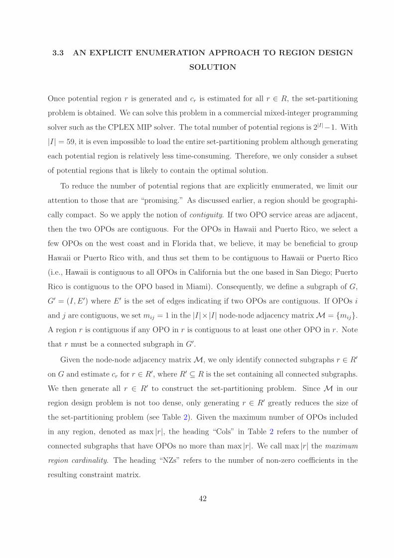
3.3 AN EXPLICIT ENUMERATION APPROACH TO REGION DESIGN
SOLUTION
Once potential region r is generated and cr is estimated for all r ∈ R, the set-partitioning
problem is obtained. We can solve this problem in a commercial mixed-integer programming
solver such as the CPLEX MIP solver. The total number of potential regions is 2|I|−1. With
|I| = 59, it is even impossible to load the entire set-partitioning problem although generating
each potential region is relatively less time-consuming. Therefore, we only consider a subset
of potential regions that is likely to contain the optimal solution.
To reduce the number of potential regions that are explicitly enumerated, we limit our
attention to those that are “promising.” As discussed earlier, a region should be geographi-
cally compact. So we apply the notion of contiguity. If two OPO service areas are adjacent,
then the two OPOs are contiguous. For the OPOs in Hawaii and Puerto Rico, we select a
few OPOs on the west coast and in Florida that, we believe, it may be beneficial to group
Hawaii or Puerto Rico with, and thus set them to be contiguous to Hawaii or Puerto Rico
(i.e., Hawaii is contiguous to all OPOs in California but the one based in San Diego; Puerto
Rico is contiguous to the OPO based in Miami). Consequently, we define a subgraph of G,
G′ = (I, E ′) where E ′ is the set of edges indicating if two OPOs are contiguous. If OPOs i
and j are contiguous, we set mij = 1 in the |I|×|I| node-node adjacency matrixM = {mij}.
A region r is contiguous if any OPO in r is contiguous to at least one other OPO in r. Note
that r must be a connected subgraph in G′.
Given the node-node adjacency matrixM, we only identify connected subgraphs r ∈ R′
on G and estimate cr for r ∈ R′, where R′ ⊆ R is the set containing all connected subgraphs.
We then generate all r ∈ R′ to construct the set-partitioning problem. Since M in our
region design problem is not too dense, only generating r ∈ R′ greatly reduces the size of
the set-partitioning problem (see Table 2). Given the maximum number of OPOs included
in any region, denoted as max |r|, the heading “Cols” in Table 2 refers to the number of
connected subgraphs that have OPOs no more than max |r|. We call max |r| the maximum
region cardinality. The heading “NZs” refers to the number of non-zero coefficients in the
resulting constraint matrix.
42
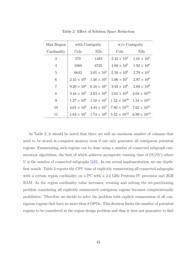
Table 2: Effect of Solution Space Reduction
Max Region with Contiguity w/o Contiguity
Cardinality Cols NZs Cols NZs
3 578 1485 3.42× 10⁴ 1.01× 10⁵
4 1888 6725 4.89× 10⁵ 1.92× 10⁶
5 6643 3.05× 10⁴ 5.50× 10⁶ 2.70× 10⁷
6 2.45× 10⁴ 1.38× 10⁵ 5.06× 10⁷ 2.97× 10⁸
7 9.20× 10⁴ 6.10× 10⁵ 3.92× 10⁸ 2.69× 10⁹
8 3.44× 10⁵ 2.63× 10⁶ 2.61× 10⁹ 2.04× 10¹⁰
9 1.27× 10⁶ 1.10× 10⁷ 1.52× 10¹⁰ 1.34× 10¹¹
10 4.61× 10⁶ 4.44× 10⁷ 7.80× 10¹⁰ 7.62× 10¹¹
11 1.64× 10⁷ 1.74× 10⁸ 5.52× 10¹² 6.99× 10¹³
In Table 2, it should be noted that there are still an enormous number of columns that
need to be stored in computer memory even if one only generates all contiguous potential
regions. Enumerating such regions can be done using a number of connected subgraph enu-
meration algorithms, the best of which achieves asymptotic running time of O(|I|V ) where
V is the number of connected subgraphs [121]. In our actual implementation, we use depth-
first search. Table 3 reports the CPU time of explicitly enumerating all connected subgraphs
with a certain region cardinality on a PC with a 2.4 GHz Pentium IV processor and 2GB
RAM. As the region cardinality value increases, creating and solving the set-partitioning
problem considering all explicitly enumerated contiguous regions becomes computationally
prohibitive. Therefore we decide to solve the problem with explicit enumeration of all con-
tiguous regions that have no more than 8 OPOs. This decision limits the number of potential
regions to be considered in the region design problem and thus it does not guarantee to find
43

the optimal regional configuration. However, we are able to justify that the current regional
configuration is suboptimal even though there is a region in the southeast that contains 12
OPOs in the current configuration.
Table 3: Connected Subgraph Enumeration
Region Cardinality 5 6 7 8 9 10 11 12
# of Regions 4.8e3 1.8e4 6.7e4 2.5e5 9.3e5 3.3e6 1.2e7 ??
Enumeration Time (s) 12 114 931 6302 39008 > 2 days > 10 days ??
We design two sets of experiments where the number of regions in the optimal regional
configuration is fixed to 11 in one set and not restricted in the other set. In each experiment
set, we use 6 data sets to construct instances. With each data set, we consider the two
optional functional relationships between PNF and CIT, i.e., linear and 3rd-degree poly-
nomial. Besides solving an optimal region design instance with one of the two functional
relationships and with organ and patient numbers from a particular year between 1999 and
2002, we design two additional experiments given a set of organ arrival and patient listing
data over multiple years. One experiment is using weighted organ arrival and patient listing
numbers over a 4-year period between 1999 and 2002. The weights assigned to those years
are 0.1 to 1999, 0.2 to 2000, 0.3 to 2001, and 0.4 to 2002. The other one is using the averages
of predicted organ arrival and patient listing numbers over the next 10 years (2006 - 2015).
We fit organ and patient numbers from the past in a linear regression model and predict
those numbers in the next 10 years. Table 4 lists the description of each data set.
Given each data set and one functional relationship between PNF and CIT, we solve the
resulting instance and report in Table 5 the relative system benefit improvement through
region reorganization, compared with the current regional configuration. It also reports the
number of regions in each optimal regional configuration for the second set of experiments.
Table 5 indicates that the relative improvement is similar among various data set and the
number of regions in the optimal regional configuration is almost constant. The table shows
modest gains resulting from reorganizing the regions. Part of the reason is that primary
non-function is insensitive to the change of cold ischemia time. Only a small proportion of
44
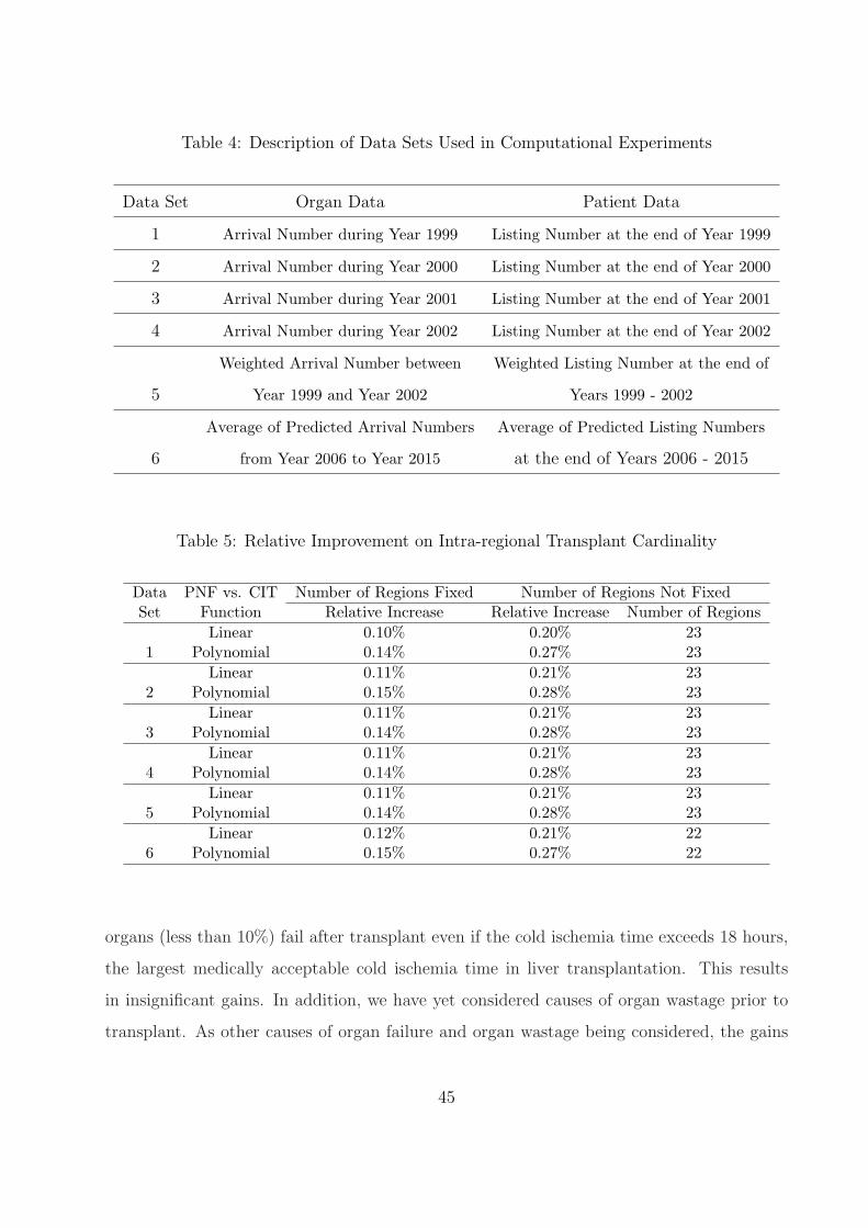
Table 4: Description of Data Sets Used in Computational Experiments
Data Set Organ Data Patient Data
1 Arrival Number during Year 1999 Listing Number at the end of Year 1999
2 Arrival Number during Year 2000 Listing Number at the end of Year 2000
3 Arrival Number during Year 2001 Listing Number at the end of Year 2001
4 Arrival Number during Year 2002 Listing Number at the end of Year 2002
Weighted Arrival Number between Weighted Listing Number at the end of
5 Year 1999 and Year 2002 Years 1999 - 2002
Average of Predicted Arrival Numbers Average of Predicted Listing Numbers
6 from Year 2006 to Year 2015 at the end of Years 2006 - 2015
Table 5: Relative Improvement on Intra-regional Transplant Cardinality
Data PNF vs. CIT Number of Regions Fixed Number of Regions Not FixedSet Function Relative Increase Relative Increase Number of Regions
Linear 0.10% 0.20% 231 Polynomial 0.14% 0.27% 23
Linear 0.11% 0.21% 232 Polynomial 0.15% 0.28% 23
Linear 0.11% 0.21% 233 Polynomial 0.14% 0.28% 23
Linear 0.11% 0.21% 234 Polynomial 0.14% 0.28% 23
Linear 0.11% 0.21% 235 Polynomial 0.14% 0.28% 23
Linear 0.12% 0.21% 226 Polynomial 0.15% 0.27% 22
organs (less than 10%) fail after transplant even if the cold ischemia time exceeds 18 hours,
the largest medically acceptable cold ischemia time in liver transplantation. This results
in insignificant gains. In addition, we have yet considered causes of organ wastage prior to
transplant. As other causes of organ failure and organ wastage being considered, the gains
45

should enlarge. Even modest gains, however, may substantially change the transplantation
environment. Annually, there are approximately 1200 end-stage liver disease patients in
the most urgent clinical categories on the waiting lists nationwide and less than 400 with a
projected life expectancy of less than 1 month. On any given day there are typically less
than 20 patients in this most urgent category [106]. This has been relative stable for the
past several years. An additional 10 or so (0.2 – 0.3% improvement) transplants/year could
save the lives of 2.5% of those in most urgent need category. Consequently, it could shift the
profile of the overall transplant waiting list towards the less ill and start reducing the length
of the waiting list.
We show optimal configurations in various instances in Figures 5 – 8. The first two sets
of figures show various optimal regional configurations in our first experiment set. The other
two sets of figures show the optimal configurations in our second experiment set. These
figures show that the regional configuration does not change or sightly changes given various
data sets. For a given set of organ and patient numbers, the optimal regional configuration
remains the same regardless of the analytic function of PNF vs. CIT. This suggests that
regional reconfiguration is insensitive to the relationship between organ viability loss and
organ transport distance. Another observation is that most of the regions consist of 2 or
3 OPOs in all optimal regional configurations when the number of regions in an optimal
configuration is not fixed.
Figures 7 - 8 indicate that in this model, the optimal regional configuration tend to
group densely populated areas. For example, unlike the current configuration, all optimal
configurations have the New England area, the New York/New Jersey metropolitan area,
and the Philadelphia/Baltimore/DC metropolitan area appear in three separate regions,
respectively, without inclusion of any other area. When the number of regions in the optimal
configuration is fixed to 11, Figures 5 - 6 show that all optimal configurations group the New
England area, the states of New York and New Jersey, and eastern Pennsylvania together
whereas most of the northern portion of central U.S. is in one region. This suggests that the
benefit of grouping more densely populated areas, i.e., the resulting increase of intra-regional
transplants in more densely populated areas, tends to outweigh any losses from having large,
46
Figure 5: Optimal Regional Configuration (PNF vs. CIT: Linear; The number of regions is
fixed to 11)
47

Figure 6: Optimal Regional Configuration (PNF vs. CIT: 3rd-degree Polynomial; The
number of regions is fixed to 11)
48

Figure 7: Optimal Regional Configuration (PNF vs. CIT: Linear; The number of regions is
unrestricted)
49

Figure 8: Optimal Regional Configuration (PNF vs. CIT: 3rd-degree Polynomial; The
number of regions is unrestricted)
50

less densely populated areas. This also implies that there is inequitable distribution of organs
in terms of organ viability across OPOs, which is one phenomenon of geographic inequity.
In the next section, we address the issue of geographic equity.
3.4 INCORPORATING GEOGRAPHIC EQUITY
Table 6: Discrepancy on Intra-regional Transplant Rate with Optimal Configuration
Data PNF vs. CIT Number of Regions Fixed Number of Regions Not FixedSet Function Max : Min Max OPO∗ Min OPO∗∗ Max : Min Max OPO∗ Min OPO∗∗
Linear 258 : 1 CAGS CADN 405 : 1 CTOP CADN1 Polynomial 258 : 1 CAGS CADN 405 : 1 CAGS CADN
Linear 190 : 1 CAGS CADN 223 : 1 CTOP CADN2 Polynomial 190 : 1 CAGS CADN 223 : 1 CTOP CADN
Linear 305 : 1 CAGS CADN 577 : 1 NMOP CADN3 Polynomial 305 : 1 CAGS CADN 577 : 1 NMOP CADN
Linear 198 : 1 CAGS CADN 277 : 1 NMOP CADN4 Polynomial 198 : 1 CAGS CADN 277 : 1 NMOP CADN
Linear 218 : 1 CAGS CADN 292 : 1 NMOP CADN5 Polynomial 218 : 1 CAGS CADN 292 : 1 NMOP CADN
Linear 388 : 1 CAGS CADN 589 : 1 OHOV CADN6 Polynomial 388 : 1 CAGS CADN 589 : 1 OHOV CADN
*: OPO with the largest value of the geographic equity measure nationwide.**: OPO with the smallest value of the geographic equity measure nationwide.
As discussed above, geographic inequity reflects on the disparity of organ transport
distances across OPOs. More importantly, geographic inequity reflects on the difference of
intra-regional transplant rates between OPOs. To be specific, on average, patients in some
OPOs have a higher chance to receive intra-regional transplants than in other OPOs. Here,
the intra-regional transplant rate at each OPO is defined as the intra-regional transplant
cardinality of that OPO divided by the total number of patients in that OPO. We refer it as
the geographic equality measure of the OPO. In Table 6, we present the ratio between the
largest and smallest values of the geographic equity measure given various data sets. The
table shows that there is a big discrepancy between the largest and smallest values. The
table also reports the codes of OPOs with the largest and smallest values of the geographic
equity measure. The OPO with the smallest geographic equity value is identical irrespective
to the functional relationship between PNF and CIT and the considered data set. The OPO
with the largest geographic equity value is also insensitive to the change of the functional
51
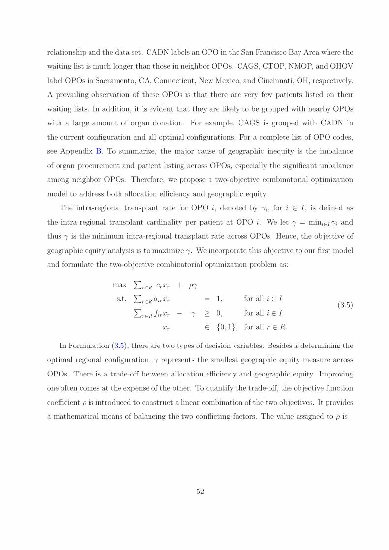
relationship and the data set. CADN labels an OPO in the San Francisco Bay Area where the
waiting list is much longer than those in neighbor OPOs. CAGS, CTOP, NMOP, and OHOV
label OPOs in Sacramento, CA, Connecticut, New Mexico, and Cincinnati, OH, respectively.
A prevailing observation of these OPOs is that there are very few patients listed on their
waiting lists. In addition, it is evident that they are likely to be grouped with nearby OPOs
with a large amount of organ donation. For example, CAGS is grouped with CADN in
the current configuration and all optimal configurations. For a complete list of OPO codes,
see Appendix B. To summarize, the major cause of geographic inequity is the imbalance
of organ procurement and patient listing across OPOs, especially the significant unbalance
among neighbor OPOs. Therefore, we propose a two-objective combinatorial optimization
model to address both allocation efficiency and geographic equity.
The intra-regional transplant rate for OPO i, denoted by γi, for i ∈ I, is defined as
the intra-regional transplant cardinality per patient at OPO i. We let γ = mini∈I γi and
thus γ is the minimum intra-regional transplant rate across OPOs. Hence, the objective of
geographic equity analysis is to maximize γ. We incorporate this objective to our first model
and formulate the two-objective combinatorial optimization problem as:
max∑
r∈R crxr + ργ
s.t.∑
r∈R airxr = 1, for all i ∈ I∑
r∈R firxr − γ ≥ 0, for all i ∈ I
xr ∈ {0, 1}, for all r ∈ R.
(3.5)
In Formulation (3.5), there are two types of decision variables. Besides x determining the
optimal regional configuration, γ represents the smallest geographic equity measure across
OPOs. There is a trade-off between allocation efficiency and geographic equity. Improving
one often comes at the expense of the other. To quantify the trade-off, the objective function
coefficient ρ is introduced to construct a linear combination of the two objectives. It provides
a mathematical means of balancing the two conflicting factors. The value assigned to ρ is
52

based on how much importance we place on geographic equity versus allocation efficiency.
In the formulation, the intra-regional transplant rate of OPO i given i ∈ Ir, denoted by fir,
is defined as:
fir =∑
j∈Ir,j 6=i
oj ·1
∑
k∈Ir,k 6=j pk
· αji. (3.6)
If a potential region r is chosen, γi = fir for i ∈ Ir. With the assumption that pi is positive
for all i ∈ I, we know γi is positive. In reality, we set γi to be 0 if (3.6) cannot be evaluated.
In Formulation (3.5), constraints∑
r∈R firxr − γ ≥ 0 for all i ∈ I, restrict γ to be equal to
the smallest value of γi for all i ∈ I. In the same manner as for the first model, we design
two sets of experiments where the number of regions in the optimal regional configuration
is fixed to 11 in one set and not restricted in the other set. We consider the same six
sets of organ procurement and patient listing data. We assign the value of ρ to be 100k,
k = 0, 1, . . . , 10. Note that Formulation (3.1) is a special case of Formulation (3.5). In
the case where k = 0, Formulation (3.5) is reduced to Formulation (3.1). We define ρc
to be the total intra-regional transplant cardinality divided by the minimum intra-regional
transplant rate, given the current regional configuration. The value of ρc in various cases are
recorded in Table 7. It can be understood as a value with which a decision maker under the
current condition would be indifferent between increasing the total intra-regional transplant
cardinality by 1 and increasing the minimum intra-regional transplant rate by 1ρc
. We also
run experiments where ρ = ρc.
Table 7: The Value of ρc
PNF Data Setvs. CIT 1 2 3 4 5 6Linear 1.742 ×10⁵ 1.310 ×10⁵ 1.659 ×10⁵ 1.270 ×10⁵ 1.425 ×10⁵ 1.749 ×10⁵
Polynomial 1.740 ×10⁵ 1.309 ×10⁵ 1.657 ×10⁵ 1.269 ×10⁵ 1.423 ×10⁵ 1.749 ×10⁵
Table 8 reports the relative improvement on the overall objective in Formulation (3.5).
For the cases where the number of regions in the optimal configuration is not restricted, it
also reports that number. Figures 9 - 12 present Pareto frontiers in four different cases. In
these figures, we also show the allocation efficiency and geographic equity measures with the
current regional configuration. Figures 13 and 14 compare two objectives separately between
53
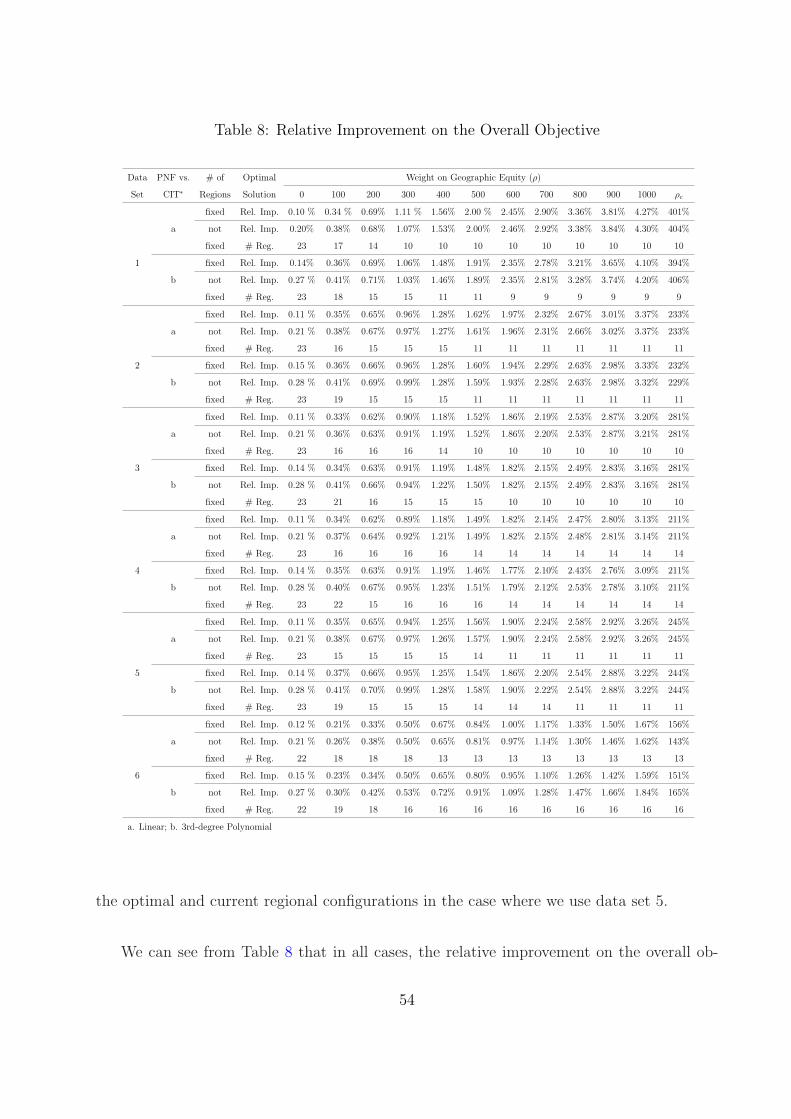
Table 8: Relative Improvement on the Overall Objective
Data PNF vs. # of Optimal Weight on Geographic Equity (ρ)
Set CIT∗ Regions Solution 0 100 200 300 400 500 600 700 800 900 1000 ρc
fixed Rel. Imp. 0.10 % 0.34 % 0.69% 1.11 % 1.56% 2.00 % 2.45% 2.90% 3.36% 3.81% 4.27% 401%
a not Rel. Imp. 0.20% 0.38% 0.68% 1.07% 1.53% 2.00% 2.46% 2.92% 3.38% 3.84% 4.30% 404%
fixed # Reg. 23 17 14 10 10 10 10 10 10 10 10 10
1 fixed Rel. Imp. 0.14% 0.36% 0.69% 1.06% 1.48% 1.91% 2.35% 2.78% 3.21% 3.65% 4.10% 394%
b not Rel. Imp. 0.27 % 0.41% 0.71% 1.03% 1.46% 1.89% 2.35% 2.81% 3.28% 3.74% 4.20% 406%
fixed # Reg. 23 18 15 15 11 11 9 9 9 9 9 9
fixed Rel. Imp. 0.11 % 0.35% 0.65% 0.96% 1.28% 1.62% 1.97% 2.32% 2.67% 3.01% 3.37% 233%
a not Rel. Imp. 0.21 % 0.38% 0.67% 0.97% 1.27% 1.61% 1.96% 2.31% 2.66% 3.02% 3.37% 233%
fixed # Reg. 23 16 15 15 15 11 11 11 11 11 11 11
2 fixed Rel. Imp. 0.15 % 0.36% 0.66% 0.96% 1.28% 1.60% 1.94% 2.29% 2.63% 2.98% 3.33% 232%
b not Rel. Imp. 0.28 % 0.41% 0.69% 0.99% 1.28% 1.59% 1.93% 2.28% 2.63% 2.98% 3.32% 229%
fixed # Reg. 23 19 15 15 15 11 11 11 11 11 11 11
fixed Rel. Imp. 0.11 % 0.33% 0.62% 0.90% 1.18% 1.52% 1.86% 2.19% 2.53% 2.87% 3.20% 281%
a not Rel. Imp. 0.21 % 0.36% 0.63% 0.91% 1.19% 1.52% 1.86% 2.20% 2.53% 2.87% 3.21% 281%
fixed # Reg. 23 16 16 16 14 10 10 10 10 10 10 10
3 fixed Rel. Imp. 0.14 % 0.34% 0.63% 0.91% 1.19% 1.48% 1.82% 2.15% 2.49% 2.83% 3.16% 281%
b not Rel. Imp. 0.28 % 0.41% 0.66% 0.94% 1.22% 1.50% 1.82% 2.15% 2.49% 2.83% 3.16% 281%
fixed # Reg. 23 21 16 15 15 15 10 10 10 10 10 10
fixed Rel. Imp. 0.11 % 0.34% 0.62% 0.89% 1.18% 1.49% 1.82% 2.14% 2.47% 2.80% 3.13% 211%
a not Rel. Imp. 0.21 % 0.37% 0.64% 0.92% 1.21% 1.49% 1.82% 2.15% 2.48% 2.81% 3.14% 211%
fixed # Reg. 23 16 16 16 16 14 14 14 14 14 14 14
4 fixed Rel. Imp. 0.14 % 0.35% 0.63% 0.91% 1.19% 1.46% 1.77% 2.10% 2.43% 2.76% 3.09% 211%
b not Rel. Imp. 0.28 % 0.40% 0.67% 0.95% 1.23% 1.51% 1.79% 2.12% 2.53% 2.78% 3.10% 211%
fixed # Reg. 23 22 15 16 16 16 14 14 14 14 14 14
fixed Rel. Imp. 0.11 % 0.35% 0.65% 0.94% 1.25% 1.56% 1.90% 2.24% 2.58% 2.92% 3.26% 245%
a not Rel. Imp. 0.21 % 0.38% 0.67% 0.97% 1.26% 1.57% 1.90% 2.24% 2.58% 2.92% 3.26% 245%
fixed # Reg. 23 15 15 15 15 14 11 11 11 11 11 11
5 fixed Rel. Imp. 0.14 % 0.37% 0.66% 0.95% 1.25% 1.54% 1.86% 2.20% 2.54% 2.88% 3.22% 244%
b not Rel. Imp. 0.28 % 0.41% 0.70% 0.99% 1.28% 1.58% 1.90% 2.22% 2.54% 2.88% 3.22% 244%
fixed # Reg. 23 19 15 15 15 14 14 14 11 11 11 11
fixed Rel. Imp. 0.12 % 0.21% 0.33% 0.50% 0.67% 0.84% 1.00% 1.17% 1.33% 1.50% 1.67% 156%
a not Rel. Imp. 0.21 % 0.26% 0.38% 0.50% 0.65% 0.81% 0.97% 1.14% 1.30% 1.46% 1.62% 143%
fixed # Reg. 22 18 18 18 13 13 13 13 13 13 13 13
6 fixed Rel. Imp. 0.15 % 0.23% 0.34% 0.50% 0.65% 0.80% 0.95% 1.10% 1.26% 1.42% 1.59% 151%
b not Rel. Imp. 0.27 % 0.30% 0.42% 0.53% 0.72% 0.91% 1.09% 1.28% 1.47% 1.66% 1.84% 165%
fixed # Reg. 22 19 18 16 16 16 16 16 16 16 16 16
a. Linear; b. 3rd-degree Polynomial
the optimal and current regional configurations in the case where we use data set 5.
We can see from Table 8 that in all cases, the relative improvement on the overall ob-
54

Figure 9: Pareto Frontier – Geographic Equity vs. Allocation Efficiency (PNF vs. CIT:
Linear; The number of regions is fixed to 11)
55

Figure 10: Pareto Frontier – Geographic Equity vs. Allocation Efficiency (PNF vs. CIT:
3rd-degree Polynomial; The number of regions is fixed to 11)
56
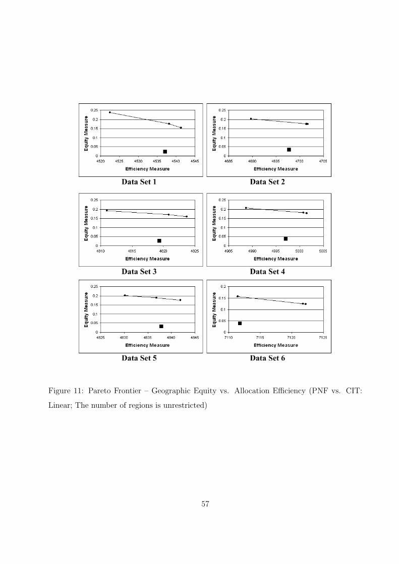
Figure 11: Pareto Frontier – Geographic Equity vs. Allocation Efficiency (PNF vs. CIT:
Linear; The number of regions is unrestricted)
57

Figure 12: Pareto Frontier – Geographic Equity vs. Allocation Efficiency (PNF vs. CIT:
3rd-degree Polynomial; The number of regions is unrestricted)
58

Figure 13: Optimal Configuration vs. Current Configuration (The number of regions is fixed
to 11)
59

Figure 14: Optimal Configuration vs. Current Configuration (The number of regions is
unrestricted)
60
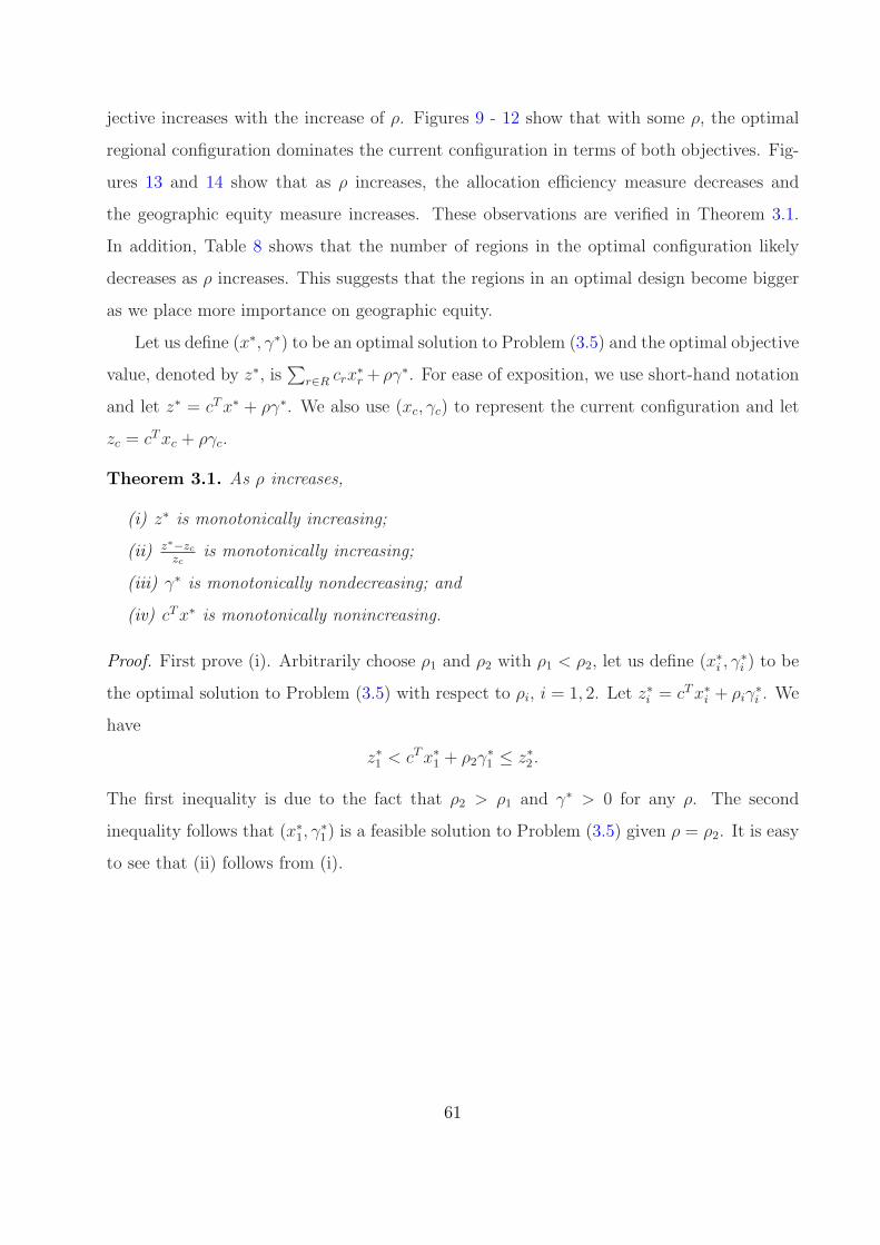
jective increases with the increase of ρ. Figures 9 - 12 show that with some ρ, the optimal
regional configuration dominates the current configuration in terms of both objectives. Fig-
ures 13 and 14 show that as ρ increases, the allocation efficiency measure decreases and
the geographic equity measure increases. These observations are verified in Theorem 3.1.
In addition, Table 8 shows that the number of regions in the optimal configuration likely
decreases as ρ increases. This suggests that the regions in an optimal design become bigger
as we place more importance on geographic equity.
Let us define (x∗, γ∗) to be an optimal solution to Problem (3.5) and the optimal objective
value, denoted by z∗, is∑
r∈R crx∗r + ργ∗. For ease of exposition, we use short-hand notation
and let z∗ = cT x∗ + ργ∗. We also use (xc, γc) to represent the current configuration and let
zc = cT xc + ργc.
Theorem 3.1. As ρ increases,
(i) z∗ is monotonically increasing;
(ii) z∗−zc
zcis monotonically increasing;
(iii) γ∗ is monotonically nondecreasing; and
(iv) cT x∗ is monotonically nonincreasing.
Proof. First prove (i). Arbitrarily choose ρ1 and ρ2 with ρ1 < ρ2, let us define (x∗i , γ
∗i ) to be
the optimal solution to Problem (3.5) with respect to ρi, i = 1, 2. Let z∗i = cT x∗i + ρiγ
∗i . We
have
z∗1 < cT x∗1 + ρ2γ
∗1 ≤ z∗2 .
The first inequality is due to the fact that ρ2 > ρ1 and γ∗ > 0 for any ρ. The second
inequality follows that (x∗1, γ
∗1) is a feasible solution to Problem (3.5) given ρ = ρ2. It is easy
to see that (ii) follows from (i).
61

Let us now prove (iii) and (iv). By the definition of (x∗1, γ
∗1) and (x∗
2, γ∗2), we have the
following two inequalities:
cT x∗1 + ρ2γ
∗1 ≤ z∗2 = cT x∗
2 + ρ2γ∗2 and
cT x∗1 + ρ1γ
∗1 = z∗1 ≥ cT x∗
2 + ρ1γ∗2 .
(iii) and (iv) follow from obtaining the difference of two left-hand sides and the difference of
two right-hand sides in the above inequalities.
Finally in this section, we show the reduction of geographic inequity in Table 9. Theorem
3.1 states that the geographic equity measure does not decrease as ρ increases. Hence, we
report the case where ρ = 1000. Table 9 is set up in the same way as Table 6. From the
table, it is clear that the discrepancy on geographic inequity is significantly reduced. In
addition, the OPOs with the largest or smallest geographic equity values tend to differ more
among the data sets.
Table 9: Reduction of Geographic Inequity when ρ = 103
PNF vs. CIT Number of Regions Fixed Number of Regions Not FixedFunction Max : Min Max OPO∗ Min OPO∗∗ Max : Min Max OPO∗ Min OPO∗∗
Year Linear 5.57 : 1 FLWC CAOP 4.43 : 1 TNMS ILIP1999 Polynomial 5.23 : 1 FLWC ILIP 2.90 : 1 FLWC CAOPYear Linear 7.11 : 1 TNMS MAOB 7.09 : 1 TNMS ILIP2000 Polynomial 7.12 : 1 TNMS CAOP 4.31 : 1 OHOV CAOPYear Linear 5.92 : 1 TNMS CAOP 4.11 : 1 NCCM CAOP2001 Polynomial 8.37 : 1 TNMS CAOP 4.12 : 1 NCCM CAOPYear Linear 3.87 : 1 OHOV PADV 7.29 : 1 TNMS CAOP2002 Polynomial 6.21 : 1 OKOP CAOP 7.30 : 1 TNMS CAOP
Weighted Linear 6.91 : 1 TNMS PADV 5.10 : 1 OHOV CAOP1999-2002 Polynomial 8.22 : 1 TNMS CAOP 5.11 : 1 OHOV CAOPAverage Linear 14.4 : 1 OHOV CAOP 12.3 : 1 NCCM ILIP
2006-2015 Polynomial 14.2 : 1 MWOB PADV 12.0 : 1 TNMS ILIP*: OPO with the largest value of the geographic equity measure nationwide.**: OPO with the smallest value of the geographic equity measure nationwide.
3.5 DEFICIENCIES AND FURTHER CONSIDERATIONS
Table 5 indicates that most of the regions consist of few OPOs in the optimal regional con-
figuration if the number of regions is not restricted. This implies that the effect of having
62
large regions on transplantable organ utilization is not fully realized. On the other hand,
the effect of having small regions on preventing organ viability loss is noticeable. The reason
for this is twofold. First, in Stahl et al. [195] all organs are considered to be accepted at
the end of Phase 4. The organs are either transplanted or wasted due to quality decay. In
other words, no organ is made available at the national level. Second, the individual-organ
benefit would decrease as the recipient OPO is farther away from the procurement OPO.
Hence, there is no incentive for an OPO to either seek many other OPOs to group with
or seek another OPO somewhere far away to group with. To some extend, the solution is
seeking a maximum weighted matching solution. A further consideration is to refine the
estimation presented in this chapter to incorporate organ usage at the national level so that
larger regions may be more beneficial, which is consistent with the recommendation made by
experts on organ procurement and transplantation policy in the DHHS Final Rule. Incorpo-
rating national-level usage in the estimation will potentially lead to larger improvement in
transplant allocation efficiency as well. Stahl et al. [195] modeled procured organs and listed
patients as homogeneous groups. However, the clinical and demographic characteristics of
donors and patients vary greatly across the country. A further consideration is to refine the
estimation presented in this chapter to reflect this fact. We will discuss a refined estimation
model in Chapter 4.
When constructing the input of the set-partitioning problem, we explicitly enumerate
potential regions. Therefore, in our straightforward solution of the region design problem, we
have to limit the number of considered potential regions by only selecting contiguous regions
with no more than a certain number of OPOs. Obviously, the obtained optimal regional
configuration cannot be proved optimal over all potential configurations. This motivates us
to apply more sophisticated solution methods. We will present an application of branch and
price in Chapter 5.
In the following chapters, we will only consider the set-partitioning model and won’t
further address the issue of geographic equity. From a modeling point of viewpoint, it is
straightforward to incorporate the equity measure into the modeling framework. However,
the incorporation will present additional challenge in solution that cannot be resolved with
the branch-and-price algorithm presented in Chapter 5.
63

4.0 OPTIMIZING INTRA-REGIONAL TRANSPLANTATION WITH TWO
MODEL REFINEMENTS THROUGH EXPLICIT ENUMERATION OF
REGIONS
As briefly stated in Chapter 3.5 “Deficiencies and Further Considerations,” the models in
Chapter 3 assume that all organs are transplanted or wasted at the end of Phase 4. In other
words, we do not address the effect of national-level allocation on regional-level allocation.
Those models also assume that all organs and patients are from the same homogeneous
groups. It is, however, evident that neither organ procurement nor patient listing follows the
same distribution across OPOs. In Section 4.1, we first elaborate on the critique of these two
assumptions and motivate two corresponding refinements of the first model from Chapter 3.
Then we present a refined model in Section 4.2 that attempts to address the effect of national-
level allocation and heterogeneity of organ procurement and patient listing. Our purpose in
this chapter is to develop a more accurate and realistic analytic model for the optimal region
design problem. The refined model requires parameter estimation using a clinically based
organ transplantation and allocation simulation model developed in Shechter et al. [188].
We discuss issues related to our parameter estimation in Section 4.3. After constructing the
model, we solve various instances using the explicit region enumeration method described in
Chapter 3 and present our solutions in Section 4.4. We then verify the solutions in Section
4.5 based on the same simulation model. In Section 4.6, we attempt to apply a modeling
technique borrowed from airline fleet assignment [104] to model the allocation at the national
level within the framework we have presented. At the end of this chapter, we summarize all
necessary assumptions made in the latest model.
64

4.1 CRITIQUE OF THE FIRST MODEL IN CHAPTER 3
An observation made from the solutions of the first model in Chapter 3 (Stahl et al. [195])
is that there are many small regions in the optimal regional configuration if the number of
regions in the optimal solution is not restricted. The reason that small regions are preferable
in that model is because the model does not fully capture the benefit that larger regions
would create a larger organ donation pool and a larger patient waiting pool. It is evident
that as the region size grows, more donor-recipient pairs would exist, more transplants would
occur at the regional level, and it would be more likely that a patient accepts an organ offer.
Furthermore, the model provides solutions that conflict with the one recommendation made
in the DHHS Final Rule [158] that suggests Organ Allocation Areas be established to serve a
population base of at least 9 million people. There are approximately 30% of regions that do
not satisfy the recommendation (Populations in OPO service areas are estimated based on
U.S Census 2000 [38]). Here are a few regions from an optimal regional configuration, based
on the regional benefit estimate in Chapter 3 (see (3.2)), that consist of a population less than
9 million: New Mexico and Arizona (NMOP & AZOB), 7 millions; Iowa and Missouri (IAOP
& MOMA), 8.5 million; Kansas and Nebraska (MWOB & NEOR), 4.4 million; and Colorado,
Utah, and Southern Idaho (CORS & UTOP), 7.2 million. See Table 10 for population in
the selected OPO service areas.
Table 10: OPO Service Areas with Population of Less than 9 Million
OPO Code NMOP AZOB IAOP MOMA MWOB NEOR CORS UTOPPopulation (in millions) 1.8 5.2 2.9 5.6 2.7 1.7 4.3 2.9
To capture the benefit accrued with the increase of region size, we need to incorporate
the effect of national-level allocation on the allocation at the regional level. The simplest way
to model the national effect is to set a fraction of organs that will not be accepted or wasted
by any patient and will be made available at the national level. This fraction is conceivably
dependent upon the donor OPO and what region is chosen to contain the OPO. This idea
65

is analogous to spill and recapture [122] considered in the airline fleet assignment problem
[104] to address the issue of an assigned aircraft for a flight not being able to accommodate
every passenger.
Previously we modeled that organ procurement and patient listing are geographically
homogeneous. However, the clinical and demographic characteristics of donors and patients
vary greatly across the country. A more realistic model must reflect this fact. To see how
modeling the clinical and demographic characteristics can influence the selection of regions,
we refer to Table 11, in which we compare a few clinical and demographic characteristics
of deceased liver donors and liver disease patients in four selected OPOs. In the table, the
deceased donor data are based on UNOS data from year 2004 and the patient data are based
on UNOS data as of October 20, 2005.
Table 11: Difference in Clinical and Demographic Characteristics Pertaining to Liver Trans-
plantation
Deceased Donor OPO Patient OPOCharacteristics Classification HIOP1 GALL2 CAOP3 MAOB4 HIOP GALL CAOP MAOB
White 33.3% 63.0% 36.9% 78.7% 34.4% 83.3% 49.7% 87.2%Black 0 30.1% 11.8% 5.8% 0 12.5% 3.8% 3.2%
Ethnicity Hispanic 0 5.6% 37.6% 12.9 % 3.1% 1.9% 36.4% 6.4%Others 66.7% 1.4% 13.6% 2.6% 62.5% 2.3% 10.1% 3.2%
O 50.0% 50.0% 50.2% 52.6% 59.4% 49.0% 53.1% 48.0%Blood A 33.3% 32.9% 31.9% 34.9% 18.8% 39.3% 33.2% 37.4%Type B 16.7% 13.4% 15.4% 9.7% 15.6% 9.7% 11.2% 12.6%
AB 0 3.7% 2.5% 2.9% 6.3% 1.9% 2.6% 2.0%Status 1 0 0 0.1% 0.1%
MELD 25+ 3.1% 0.4% 3.1% 2.1%Urgency MELD 19-24 N/A 6.3% 7.4% 6.2% 4.4%Medical MELD 11-18 56.3% 52.5% 31.2% 19.8%
MELD < 10 21.9% 28.0% 42.1% 26.0%Status 7 12.5% 11.7% 17.3% 47.5%
1. An OPO serving Hawaii.2. An OPO serving Georgia.3. An OPO serving Southern California.4. An OPO serving Massachusetts.
Table 11 indicates that deceased liver donors and liver disease patients do not have the
same distributions across OPOs with respect to these clinical and demographic characteris-
tics. Different parts of the country, have markedly different racial compositions and blood
type breakdowns. For example, over 30% of donors and patients in Southern California are
Hispanic whereas Hispanic donors and patients constitute less than 6% in all other three
OPO service areas. Another example is that the proportion of African-American donors in
66

Georgia is at least twice as much as the proportion in any of other three OPOs. We can
also see in the table that the proportion of blood type A patients in Hawaii is significantly
less than that in other OPOs. Interestingly, a noticeably large proportion of patients listed
on the waiting lists in Massachusetts are inactive (Status 7) compared to other three OPOs.
This could be due to the leading transplantation facilities and personnel in that area.
To model clinical and demographic characteristics more accurately in our regional benefit
estimate, we consider the distribution of various clinical and demographic characteristics
across OPOs, such as gender, age, blood type, disease group, etc. We also apply a natural
history model of end-stage liver disease embedded in the simulation model to consider the
dynamics of disease progression.
4.2 REFINED OPTIMAL REGION DESIGN MODEL
In this section, we refine the optimal region design model presented in Chapter 3 from
two aspects motivated as above. In one aspect, we consider organ and patient flows to
the national level. With this refinement, the model is able to capture the accrued benefit of
having relatively large regions. In the other aspect, we consider geographic differences among
organs and patients. In the refined model, we only modify the regional benefit estimate and
do not change the set-partitioning framework. Since incorporating geographic equity in the
second model of Chapter 3 is independent of the regional benefit estimation, we thereby only
present the refinements for the first model in Chapter 3.
Next let us discuss how to model intra-regional organ distribution and organ flow to
the national level, for any regional configuration. Given a regional configuration, if certain
regional preference exists, a higher priority is given to organ distribution that occurs from a
donor OPO in some particular region to recipient OPOs within the same region. On the other
hand, there is a possibility that an organ will not be accepted or wasted at the regional level
and will become available at the national level. It is conceivable that different region designs
lead to different probabilities that an organ will be available at the national level. Therefore,
to develop a regional benefit estimate appropriate for any potential region, we first need to
67

exclude the effect of regional preference and thus consider organ distribution solely based on
clinical and demographic characteristics of donors and patients. This is, in fact, the situation
where the entire country has only one national waiting list for all patients. With the above
discussion regarding more accurate modeling at the regional level, we discard Assumption
A3.4 in Chapter 3, and replace Assumption A3.6, stating proportional allocation, with
assumptions as follows.
(A4.1) For intra-regional transplantation, the likelihood that an organ procured at one
OPO is accepted by a patient at each other OPO within the same potential region, is
proportional to the likelihood of organ distribution from the donor OPO to a recipient
OPO that is in the same region, where there is only a single national waiting list.
(A4.2) For organ flow to the national level, the likelihood that an organ procured at one
OPO is not accepted or wasted at the regional level (and thus made available at the
national level), is proportional to the likelihood of organ distribution to recipient OPOs
that are not included in the same region and organ wastage, when there is only a single
national waiting list.
(A4.3) Given any potential region design, the likelihood that an organ procured at one
OPO is not accepted or wasted at the regional level (and thus made available at the
national level), depends only upon the donor OPO.
Under the condition where there is a single national waiting list, we call the likelihood
of organ distribution pure distribution likelihood, and the likelihood of organ wastage and
organ distribution to all recipient OPOs that are not included in a given potential region
pure national flow likelihood. Assumptions A4.1 and A4.2 ensure proportional allocation.
Assumption A4.1 states that the higher the pure distribution likelihood is from a particular
donor OPO to a particular recipient OPO, the more intra-regional transplants occur between
the two OPOs. Assumption A4.2 states that the higher the national flow likelihood is,
the more organs procured at the donor OPO will be made available at the national level.
Assumption A4.3 is a simplifying assumption that is primarily for application of our branch-
and-price solution, which will be discussed in Chapter 5. It is conceivable that a national-level
68

flow likelihood should not depend only upon the donor OPO but also the region chosen in
the regional configuration that contains it. For a summary of necessary assumptions, we
refer forward to Section 4.7.
In Chapter 3, we assume in Assumption A3.5 that the likelihood that an organ is avail-
able for intra-regional transplantation is fixed. After observing the clinical and demographic
differences among OPOs, this likelihood is presumably dependent upon the OPO. Note that
it should still be insensitive to any region design since there are very few Status 1 patients
at Phase 2 of the allocation process.
Here is some new notation in addition to the organ number oi and organ viability measure
αij, for all i, j ∈ I. Define
• lij to be the pure distribution likelihood from donor OPO i ∈ I to recipient OPO j ∈ I.
• l0i to be the pure national flow likelihood from donor OPO i ∈ I.
• βi to be the likelihood that an organ procured at donor OPO i ∈ I is available for MELD
patients at the regional level.
Given a potential region r ∈ R, let us define Ir ⊆ I to be the set of OPOs in region r. It
is clear that if |Ir| = 1, cr = 0. Otherwise, cr is estimated as follows:
cr =∑
i∈Ir
∑
j∈Ir,j 6=i
oi · βi ·lij
∑
k∈Ir,k 6=i lik + l0i· αij. (4.1)
The explanation of the derivation of (4.1) is similar to the one in Chapter 3. Given an
organ procured at OPO i that is available at Phase 4 of the allocation process, the likelihood
it would be accepted by a matched patient at OPO j is
zij =lij
∑
k∈Ir,k 6=i lik + l0i.
Similarly, the likelihood that the organ would not be accepted or wasted at the regional level
and thus made available at the national level, denoted by z0i , is
z0i =
l0i∑
k∈Ir,k 6=i lik + l0i.
69

Let us call zij and z0i intra-regional transplant likelihood and national-level flow likelihood,
respectively. We discuss several properties of zij and z0i in the following section that help us
verify our beliefs on how the set of optimal regions looks like and demonstrate the trade-off
between larger regions and smaller regions in a region design.
Properties of Intra-regional Transplant and National-level Flow Likelihoods
In this section, we discuss how zij and z0i would behave as the pure distribution likelihood
lij increases or more OPOs are included in a region. For ease of exposition, we assume that
lij ≥ 0 and l0i > 0 for all i, j ∈ I, i 6= j.
Proposition 4.1. Given Ir ⊆ I and lij for all i, j ∈ Ir. Let zij(lij) : IR+ 7→ IR+ be a
continuous function modeling the relationship between the intra-regional transplant likelihood
and the pure distribution likelihood between donor OPO i and recipient OPO j in a considered
region, i.e.,lij
P
k∈Ir\{i} lik+l0i. Then
∑
j∈Ir\{i} zij(lij) is nondecreasing.
Proof. We know∑
j∈Ir\{i} zij(lij) =P
j∈Ir\{i} lijP
j∈Ir\{i} lij+l0i. The result follows from the fact that given
i, j ∈ I, lij is nonnegative, and l0i is fixed and positive.
Corollary 4.1. Given Ir ⊆ I and lij for all i, j ∈ Ir. Let z0i (lij) : IR+ 7→ IR+ be a continuous
function modeling the relationship between the national-level transplant likelihood from donor
OPO i and the pure distribution likelihood between donor OPO i and recipient OPO j in a
considered region, i.e.,l0i
P
k∈Ir\{i} lik+l0i. Then z0
i (lij) is nonincreasing.
Proposition 4.1 and Corollary 4.1 imply that as the pure distribution likelihood increases,
the likelihood that an organ would be accepted by a matched patient at the regional level
increases and the likelihood that it would be available at the national level decreases. In
other words, the more likely a transplant occurs between two OPOs at the regional level
where there is only a single national waiting list, the more likely that it would also occur at
the regional level when distribution is given a higher priority to the regional level than to the
national level. This is because it is easier to find donor-recipient matches at the regional level,
and thus more organs are likely to be accepted by matched patients regionally. Proposition
4.1 and Corollary 4.1 are consistent with our belief. Note that to increase the likelihood that
an organ is accepted at the regional level, it can also be achieved by forming a larger region
that includes more OPOs. This result is presented and proved in the following proposition.
70
Definition 4.1. Define fi(S) to be the function modeling the intra-regional transplantation
contribution from OPO i with respect to S such that i ∈ S ⊆ I, i.e., fi(S) =∑
j∈S\{i} zij =P
j∈S\{i} lijP
j∈S\{i} lij+l0i.
Definition 4.2. [155] Let N be a finite set, and let f be a real-valued function on the subsets
of N .
a. A function f(S) is submodular if f(S)+f(T ) ≥ f(S∪T )+f(S∩T ) for S, T ⊆ N .
b. A function f(S) is supermodular if −f is submodular.
Proposition 4.2. Given S ⊆ I, fi(S) is nondecreasing for any i ∈ S. Furthermore, if
lij = lik for all j, k ∈ I\S, j 6= k, then fi is submodular.
Proof. Let us consider a function with the following generic form f ′i(x) : IR+ 7→ [0, 1], where
x =∑
j∈S,j 6=i lij. We know
f ′i(x) =
x
x + l0i
is a continuous function. Let us define S ′ = S∪{k1} and S ′′ = S ′∪{k2} where k1 and k2 are
additional OPOs to be included in S. At discrete points x1 =∑
j∈S\{i} lij, x2 =∑
j∈S′\{i} lij,
and x3 =∑
j∈S′′\{i} lij, f ′i(·) coincides with fi(·). Clearly, f ′
i(x) is a nondecreasing and
concave function on [0, +∞) given that lij ≥ 0 and l0i > 0 for all i, j ∈ I, i 6= j. Therefore,
fi(x3)− fi(x2) ≤ fi(x2)− fi(x1) for x1 ≤ x2 ≤ x3 and x2−x1 = x3−x2, and the proposition
follows.
Definition 4.3. Define f 0i (S) to be the function modeling the national-level flow from OPO
i with respect to S such that i ∈ S ⊆ I, i.e., f 0i (S) = z0
i =l0i
P
j∈S\{i} lij+l0i.
Corollary 4.2. Given S ⊆ I, f 0i (S) is nonincreasing for any i ∈ S. Furthermore, if lij = lik
for all j, k ∈ I\S, j 6= k, then f 0i (S) is supermodular.
Remark 4.1. In both Proposition 4.2 and Corollary 4.2, the condition lij = lik for all
i, j ∈ I\S is a strong sufficient condition. In most of the cases, we are only interested in a
particular S ⊆ I. Therefore, weaker sufficient conditions can be derived when the purpose is
to study the relationship between the increase rate of intra-regional transplant contribution
or national-level flow and the region size.
71
Proposition 4.2 and Corollary 4.2 imply that as the number of OPOs in the chosen
region increases, the likelihood that an organ would be accepted by a matched patient at
the regional level increases and the likelihood that it would be available at the national
level decreases. In other words, the larger the region is, the more likely an organ would be
accepted by a matched patient at the regional level. However, in general the increase of
intra-regional transplantation contribution from one OPO would diminish as the region size
increases. Proposition 4.2 and Corollary 4.2 also match our belief.
When considering the regional benefit, we incorporate the parameter αij. Since αij is
negatively correlated to organ transport distance, it decreases as i and j are farther apart. As
derived earlier, cr =∑
i∈Ir
∑
j∈Ir,j 6=i oiβizijαij. Hence, cr may be a concave function whose
maximizer is reached as region r is of appropriate size. To summarize, the refined analytic
estimate of the regional benefit is able to capture the trade-off between organ utilization
at the regional level and organ quality decay due to transporting the organ. As a result,
most of the regions in an optimal regional configuration would appear to be compact and
middle-size.
4.3 PARAMETER ESTIMATION FOR THE REFINED MODEL
To estimate any regional benefit, the estimation of several parameters, such as organ viability
loss, and the acquisition of required data, such as the organ numbers, has been discussed in
Chapter 3. There are three other parameters in (4.1) that need to be estimated. They are
the pure distribution likelihood, lij, the pure national flow likelihood, l0i , and the likelihood
that an procured organ is available at Phase 4, βi. To estimate these parameters, we adapt
a clinically based discrete-event simulation model developed by Shechter et al. [188]. In
this section, we first describe the simulation model and how we adapt it to estimate the
necessary parameters in the model. Then we discuss our parameter estimation procedure
using the simulation model. Additional data collection will be described as the corresponding
parameter estimation is discussed.
72
4.3.1 Adaptation of a Clinically Based Simulation Model
Shechter et al. [188] designed a clinically based discrete-event simulation model to test
proposed changes in allocation policies. The authors used data from multiple sources to
simulate end-stage liver disease and the complex allocation system that includes donor and
patient generation, and organ-recipient matching.
Since their objective was to build a clinically based simulation model to test various allo-
cation policies, a discrete-event simulation model was created at the top to simulate various
matching algorithms and a Monte Carlo microsimulation model was embedded to closely
simulate the progression of various end-stage liver diseases and reflect organ procurement
and patient listing at different time points and geographic locations. The model has five core
modules: the patient generator, organ generator, pretransplant natural history, matching al-
gorithm, and posttransplant survival. For the purpose of model validation, the authors also
included several data statistical summary functions [188].
In our process of adapting the simulation model, we first update the list of OPOs since
a few OPOs became inactive after 1999. We then update several data sets in the simulation
model. They are yearly organ procurement and MELD patient listing rates, geographic
distributions of organ procurement and MELD patient listing. These updates are based on
several publicly available data sets [88]. We use data from the beginning of 1996 through
the end of 2002 whereas the model previously used data from the beginning of 1991 through
the end of 1996. To have the simulated allocation process reach steady state, we specify the
warm-up period to be from the beginning of 1996 through the end of 1998. This is based
on the consideration that we collect many other data for the period between 1999 and 2002.
By doing this, roughly the same amount of patients are generated in the simulation model
by the end of 1998, as the real patient listing data shows. There are a number of data sets
that are unable to be updated due to relevant data not being available. For the sources of
other data, see [188].
In our adaptation process, we also update the set of data statical summary functions.
We design functions that count transplants once they occur and record the year they occur
and the associated donor and recipient OPOs.
73

4.3.2 Parameter Estimation
To estimate the pure distribution likelihood, we set the matching algorithm to be such that
there is only one waiting list in the entire country and all clinically and demographically
matched patients are offered with organs based on their medical urgency. This means that
no regional preference is imposed. Thus, we believe the proportions of organs procured at
a donor OPO that are accepted by matched patients at a recipient OPO would faithfully
reflect the transplant likelihood that is solely dependent upon clinical and demographic char-
acteristics of donors and patients. In the simulation, we record the numbers of transplants
from any donor OPO to any recipient OPO. Therefore, we create an |I|×|I| matrix in which
the cell in the ith row and jth column estimates pure distribution likelihood lij.
After the above specification, we run the simulation model with 100 replications and
compute the average and standard deviation of pure distribution likelihoods over the repli-
cations. We address the statistical significance issue when determining the number of repli-
cations needed. For each pure distribution likelihood, we compute the ratio of the standard
deviation to the average over the replications. Tables 12 reports the relative frequency of the
above ratio data set. From this table, we can see that for most of the elements in the pure
distribution likelihood matrix, the ratio is less than 10%. The table also includes the largest
number on the diagonal of the matrix containing all the ratios. For some OPO pairs, the
occurrence of transplants is very rare. So their associated ratios of the standard deviation
to the average over the replications normally have large variation. But since transplants be-
tween such pairs of OPOs do not make much contribution, we do not think reducing variance
of those pairs is necessary. Therefore, running the simulation model with 100 replications
would provide conclusions with necessary statistical significance.
To estimate the pure national flow likelihood, we set the matching algorithm to be such
that certain region preference is imposed. This is done by setting some regional configuration
as input. In the simulation model, we specify a single parameter to incorporate patient
autonomy on organ acceptance/rejection. This parameter measures the probability that an
individual patient would reject an organ offer. Once an organ is generated, the simulation
follows the matching algorithm to match the organ and patients awaiting transplant. After a
74
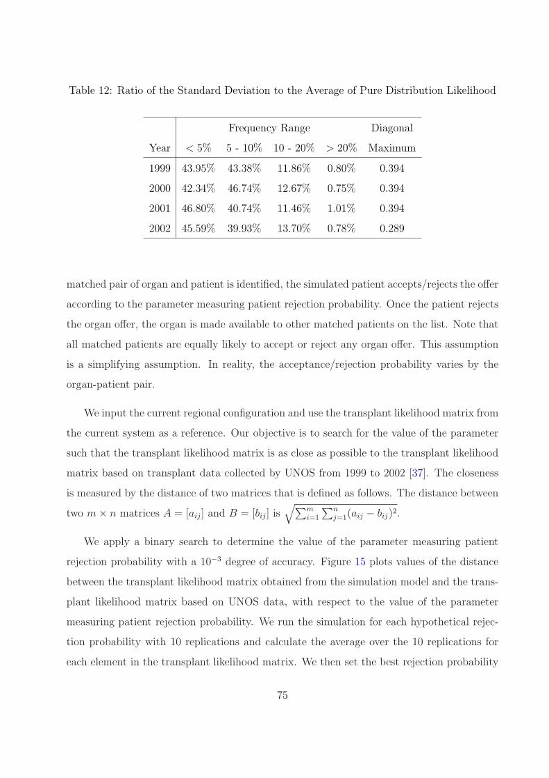
Table 12: Ratio of the Standard Deviation to the Average of Pure Distribution Likelihood
Frequency Range Diagonal
Year < 5% 5 - 10% 10 - 20% > 20% Maximum
1999 43.95% 43.38% 11.86% 0.80% 0.394
2000 42.34% 46.74% 12.67% 0.75% 0.394
2001 46.80% 40.74% 11.46% 1.01% 0.394
2002 45.59% 39.93% 13.70% 0.78% 0.289
matched pair of organ and patient is identified, the simulated patient accepts/rejects the offer
according to the parameter measuring patient rejection probability. Once the patient rejects
the organ offer, the organ is made available to other matched patients on the list. Note that
all matched patients are equally likely to accept or reject any organ offer. This assumption
is a simplifying assumption. In reality, the acceptance/rejection probability varies by the
organ-patient pair.
We input the current regional configuration and use the transplant likelihood matrix from
the current system as a reference. Our objective is to search for the value of the parameter
such that the transplant likelihood matrix is as close as possible to the transplant likelihood
matrix based on transplant data collected by UNOS from 1999 to 2002 [37]. The closeness
is measured by the distance of two matrices that is defined as follows. The distance between
two m× n matrices A = [aij] and B = [bij] is√
∑mi=1
∑nj=1(aij − bij)2.
We apply a binary search to determine the value of the parameter measuring patient
rejection probability with a 10−3 degree of accuracy. Figure 15 plots values of the distance
between the transplant likelihood matrix obtained from the simulation model and the trans-
plant likelihood matrix based on UNOS data, with respect to the value of the parameter
measuring patient rejection probability. We run the simulation for each hypothetical rejec-
tion probability with 10 replications and calculate the average over the 10 replications for
each element in the transplant likelihood matrix. We then set the best rejection probability
75
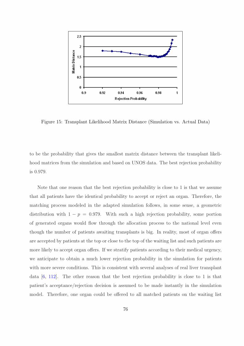
Figure 15: Transplant Likelihood Matrix Distance (Simulation vs. Actual Data)
to be the probability that gives the smallest matrix distance between the transplant likeli-
hood matrices from the simulation and based on UNOS data. The best rejection probability
is 0.979.
Note that one reason that the best rejection probability is close to 1 is that we assume
that all patients have the identical probability to accept or reject an organ. Therefore, the
matching process modeled in the adapted simulation follows, in some sense, a geometric
distribution with 1 − p = 0.979. With such a high rejection probability, some portion
of generated organs would flow through the allocation process to the national level even
though the number of patients awaiting transplants is big. In reality, most of organ offers
are accepted by patients at the top or close to the top of the waiting list and such patients are
more likely to accept organ offers. If we stratify patients according to their medical urgency,
we anticipate to obtain a much lower rejection probability in the simulation for patients
with more severe conditions. This is consistent with several analyses of real liver transplant
data [6, 112]. The other reason that the best rejection probability is close to 1 is that
patient’s acceptance/rejection decision is assumed to be made instantly in the simulation
model. Therefore, one organ could be offered to all matched patients on the waiting list
76

without any organ quality decay. In reality, an organ can only be offered to at most 5 - 10
patients before its viability is lost. If we consider in the simulation model the time taken by
each physician/patient to decide if accepting an organ offer when simulating the matching
process, we anticipate to obtain a much lower rejection probability.
We address the statistical significance issue when determining the number of replications
needed. For each hypothetical rejection probability, we compute a 95% confidence interval
for each average transplant likelihood and the ratio of the half width of the CI to the sample
average. Suppose x and s are the sample average and standard deviation of each transplant
likelihood, respectively. The ratio of the half width of the CI to the sample average is
t0.025,n−1 ·s√n/x. Figure 16 presents the maximum ratio on the diagonal of the transplant
likelihood matrix, with respect to the rejection probability value p = 0.970 + 0.001k, where
k = 0, . . . , 25. This figure shows that for all tested hypothetical rejection probability values,
the above defined ratio is below 0.3. For the chosen rejection probability, the ratio is below
0.2. The reason that we only consider ratios on the diagonal is the same as mentioned before.
Hence, we conclude that it suffices to run the simulation for 10 iterations in order to draw
statistically significant conclusions.
Figure 16: Statistical Analysis for the Rejection Probability Estimation
77

As mentioned earlier, the matching process follows, in some sense, a geometric dis-
tribution when assuming all MELD patients at the regional level have the same accep-
tance/rejection probability. We can extend this idea to analyze the entire allocation process.
We can determine each acceptance/rejection probability analytically or through simulation
for the transition at each phase. Given this probability and the number of patients await-
ing transplants at each phase, we can compute the probability that an organ will be made
available at the next phase. If an organ is used at one phase in the probabilistic sense, the
conditional regional benefit accrues accordingly. Therefore, we can compute the expected
regional benefit by summing up the 6 conditional regional benefits at all 6 phases throughout
the allocation process.
Since allocation at the regional and national levels of the allocation process is dependent
upon the regional configuration, we choose 20 potential regional configurations whose number
of regions ranges from 5 to 14. This selection is random. Our belief is that there should be
5 - 14 regions in the optimal set of regions. We set the rejection probability to be 0.979 in
the simulation and input each of the 20 regional configurations. For each configuration, we
run the simulation with 30 replications and obtain a transplant likelihood matrix. Hence for
each OPO, we have a sample of the likelihood that an organ, procured from the OPO, is
available at the national level. We then calculate the sample average over the replications
to estimate the pure national flow likelihood, l0i . To test whether using the obtained sample
average would lead to statistically significant conclusions, we compute the ratio of the sample
standard deviation to the sample average of the national flow likelihood for each OPO with
respect to a regional configuration. We report the largest ratio among OPOs in Figure 17.
The figure shows that for any chosen regional configuration, the largest ratio is below 0.1.
Hence, we conclude that it is valid to use the above pure national flow likelihood estimate
in order to draw statistically significant conclusions.
Now let us discuss how to estimate the likelihood of an organ being offered to MELD
patients at the regional level. Since this parameter does not vary much by the region design,
we calculate the proportion of organs procured at each OPO that are not transplanted to
either Status 1 patients or at the local level. In other words, we calculate the likelihood
that organs are available at Phase 4. The data set we use is generated from transplant data
78
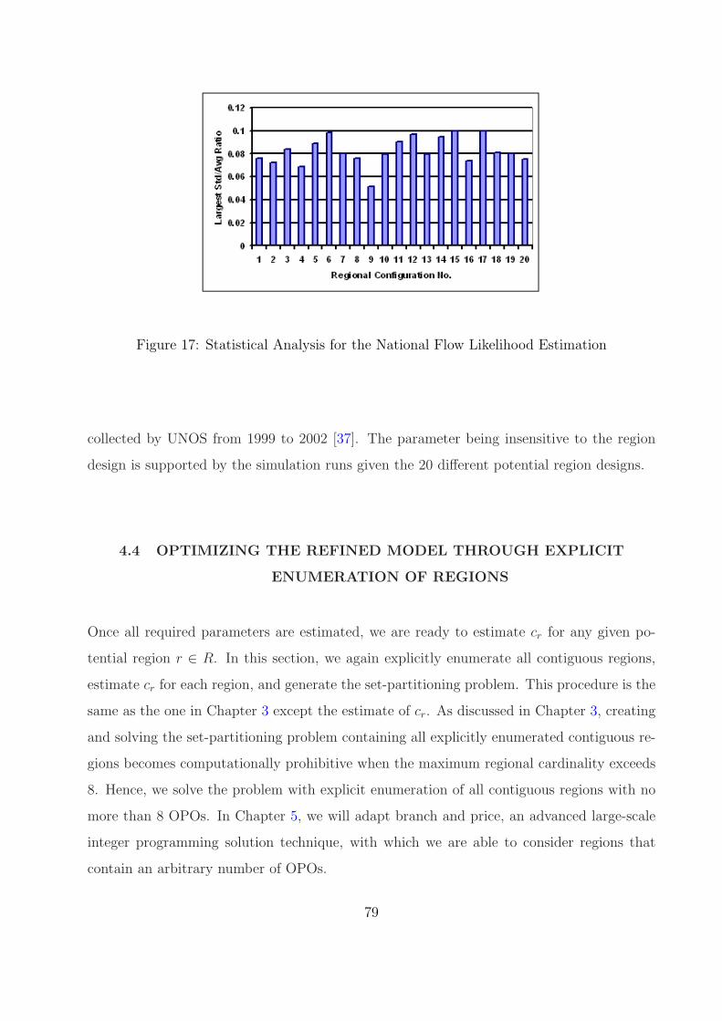
Figure 17: Statistical Analysis for the National Flow Likelihood Estimation
collected by UNOS from 1999 to 2002 [37]. The parameter being insensitive to the region
design is supported by the simulation runs given the 20 different potential region designs.
4.4 OPTIMIZING THE REFINED MODEL THROUGH EXPLICIT
ENUMERATION OF REGIONS
Once all required parameters are estimated, we are ready to estimate cr for any given po-
tential region r ∈ R. In this section, we again explicitly enumerate all contiguous regions,
estimate cr for each region, and generate the set-partitioning problem. This procedure is the
same as the one in Chapter 3 except the estimate of cr. As discussed in Chapter 3, creating
and solving the set-partitioning problem containing all explicitly enumerated contiguous re-
gions becomes computationally prohibitive when the maximum regional cardinality exceeds
8. Hence, we solve the problem with explicit enumeration of all contiguous regions with no
more than 8 OPOs. In Chapter 5, we will adapt branch and price, an advanced large-scale
integer programming solution technique, with which we are able to consider regions that
contain an arbitrary number of OPOs.
79

When contiguous regions with no more than 8 OPOs are explicitly enumerated, prelimi-
nary computational results show that the solution terminates prematurely in some instances
due to memory limitation. Therefore, we also solve the problem with all contiguous regions
with no more than 7 OPOs. In all these instances, we do not impose any constraint on
the number of regions in the optimal solution. Table 13 presents the absolute increase of
intra-regional transplant cardinality and the number of regions in the optimal regional con-
figuration. These results are consistent and encouraging. In Table 13, we also report the
Table 13: Improvement on Intra-regional Transplant Cardinality (max |r| = Maximum Re-
gion Cardinality)
max |r| = 7 max |r| = 8Data PNF vs. CIT Absolute Num. of CPU Time (s) / Absolute Num. of CPU Time (s) /Set Function Increase Regions Final LP Gap Increase Regions Final LP Gap
Linear 55.0 9 3720 69.7 8 0.37%1 Polynomial 53.4 9 5093 67.3 8 0.43%
Linear 58.8 9 11049 78.2 8 84372 Polynomial 57.2 9 8439 75.9 8 9488
Linear 57.8 9 2437 71.6 8 91963 Polynomial 56.0 9 1689 73.2 8 9900
Linear 58.0 9 6408 76.7 8 0.38%4 Polynomial 57.0 9 1035 68.9 8 0.88%
Linear 56.6 9 1026 73.6 8 0.34%5 Polynomial 54.8 9 7683 71.3 8 0.34%
Linear 86.0 9 1190 111.3 8 0.22%6 Polynomial 83.3 9 1672 109.9 8 2378
running time if CPLEX solves the instance or the terminating LP gap in branch and bound
if CPLEX terminates the solution prematurely. An integer number in the column “CPU
Time (s) / Final LP Gap” indicates an optimal solution is found and the number is the
solution time in seconds whereas a percentage indicates the solution terminates prematurely
and the number is the terminating LP gap. For all instances, the absolute increase is larger
if we allow no more than 8 OPOs in any region compared with the case where max |r| = 7.
In most of the instances, the solution time is, however, longer in the former case. There
are a few instances that CPLEX cannot solve to optimality in the former case whereas all
instances can be solved to optimality in the latter case.
One prevalent observation among the instances is that the number of regions in any
optimal regional configuration is relatively small compared to the optimal configurations
obtained from our model in Chapter 3. Figures 18 - 21 also illustrate this. Most importantly,
80
these figures show that the regions in the optimal configurations are large. Unlike the current
regional configuration, the entire Northeast is one compact region including approximately 6
- 7 OPOs in almost all instances. This implies that in an area as small as the Northeast, it is
beneficial to group more OPOs and have larger regions. Similar cases are the regions in the
Mid-Atlantic and Southeast. In almost all instances, the OPOs in California, excluding the
one serving Los Angeles and its surrounding areas (CAOP), are grouped together. The above
observations suggest that adjacent densely populated areas should be grouped together. In
almost all instances, a large region is formed in the Northwest. In some instances, this
region even contains OPOs in the Midwest. Some of the regions are not really compact as
our intuition suggests. Our explanation is as follows. First, grouping net organ supplier and
net recipient OPOs may be more critical in terms of maximizing intra-regional transplants.
Therefore, compactness becomes a secondary consideration in the solution. Second, the
locations we choose for many OPOs are not in the center of their service areas. Therefore, a
geographically less compact region does not necessarily mean fewer intra-regional transplants.
Third, gains from having some geographically compact regions may outweigh any loss from
having other geographically less compact regions together in the configuration. Note that
when inspecting Figures 18 - 21, keep in mind that we set the OPOs in Arizona and Nevada
(AZOB and NVLV) to be contiguous to the OPO in California serving Los Angeles and its
surrounding area (CAOP) and all three OPOs in Texas (TXSB, TXSA, and TXGC) to be
contiguous.
Figures 18 - 21 show that many regions in an optimal regional configuration have exactly
the same number of OPOs as the maximum number allowed in a region. For example, in
the instances where we use 1999 data and the linear function for the functional relationship
between PNF and CIT, 7 out of 9 regions have 7 OPOs when 7 is the maximum number
allowed and 5 out of 8 regions have 8 OPOs when 8 is the maximum number allowed. This
suggests that if we allow regions with even more OPOs, the regions in an optimal configura-
tion may potentially contain even more OPOs. However, as we discussed earlier, explicitly
enumerating regions becomes computationally prohibitive as the maximum regional cardi-
nality increases. Even in some cases where no more than 8 OPOs are allowed, we are able to
enumerate all potential regions and generate the set-partitioning instances but the CPLEX
81

Figure 18: Optimal Regional Configuration (PNF vs. CIT: Linear; The maximum regional
cardinality is 7)
82
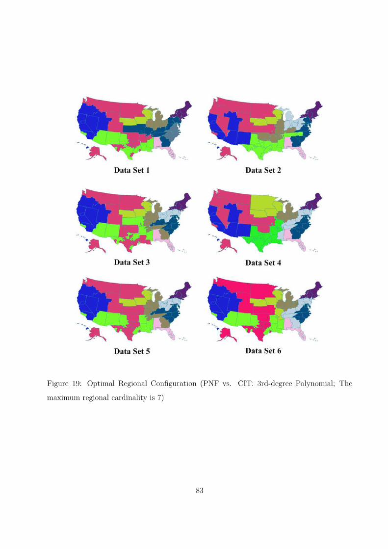
Figure 19: Optimal Regional Configuration (PNF vs. CIT: 3rd-degree Polynomial; The
maximum regional cardinality is 7)
83
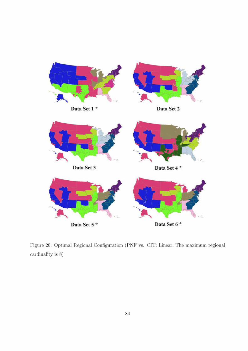
Figure 20: Optimal Regional Configuration (PNF vs. CIT: Linear; The maximum regional
cardinality is 8)
84

Figure 21: Optimal Regional Configuration (PNF vs. CIT: 3rd-degree Polynomial; The
maximum regional cardinality is 8)
85

Table 14: Improvement on Intra-regional Transplant Cardinality (through Explicit Region
Enumeration)
Data Set 1 2 3 4
Simulation 23.5 34.1 39.2 30.4
Linear Analytic 69.7 78.2 71.6 73.2
Simulation 29.7 33.2 37.0 26.6
Polynomial Analytic 67.3 75.9 73.2 68.9
branch-and-bound solution has to terminate prematurely due to memory limitation on its
branch-and-bound tree. These instances are labeled with asterisk in Figures 20 and 21.
Given the solution difficulty discussed in this chapter, we will present our application of
branch and price to improve the solution in Chapter 5.
4.5 EVALUATING THE PROPOSED REGIONS
After obtaining optimal regional configurations, we use the simulation to verify these so-
lutions. To some extend, this serves the purpose of validating the analytic model. With
some modification, the simulation model provides us the flexibility to input any regional
configuration. We run the simulation with 30 replications for each optimal regional config-
uration. The simulated time period is the same as described in Section 4.3. That is, from
the beginning of year 1996 to the end of year 2002, with the warm-up period being the first
3 years. For comparison, we also run the simulation with 30 replications for the current
regional configuration. A justification of the number of replications will be given later in
this section.
Table 14 reports the average yearly improvement on intra-regional transplant cardinality
over 30 replications from 1999 to 2002. In Table 14, we compare the improvement obtained
86

in the simulation model with that obtained in the analytic model. For example, one input
to the simulation model is the optimal regional configuration associated with data set 1.
Since data set 1 includes organ and patient numbers from 1999, we run the simulation
model over year 1999. We then compare the improvements obtained in the simulation model
and the analytic model. Similarly, we use data sets 2-4 for comparisons during years 2000,
2001, and 2002, respectively. Although the corresponding improvement numbers are not
too comparable, the simulation model verifies the improvement with the optimal regional
configuration obtained from the analytic model. To understand the different between the
two corresponding improvement numbers from the simulation and the analytic models, we
need to take a closer look at the allocation process modeled in the simulation model. The
simulation model considers the dynamics in the allocation process, particularly in the first
three phases. At Phase 3 of the allocation process, MELD patients at the local level are
assumed to reject any organ offer with a constant probability. This probability is 0.979, the
same as the rejection probability estimated earlier. As described earlier, with incorporation
of the rejection probability, we attempt to represent the transition from the regional level
to the national level in the allocation process (Phase 4 to 5) faithfully. Its estimation is
not intended to represent the transition from the local level to the regional level (Phase
3 to 4). Furthermore, since we only use one parameter to model patient autonomy, the
allocation process is sensitive to the value of the rejection probability. This creates difficulty
in estimating the parameter. The simulation result indicates that our estimate is low for the
latter transition. Thus more organs are accepted in Phase 3 than indicated by the UNOS
data [37] and thus fewer organs are made available at the regional level.
To further verify our claim that the optimal configuration increases intra-regional trans-
plant cardinality, we run paired t tests to compare the optimal regional configuration corre-
sponding to each data set and the current configuration in terms of the annual intra-regional
transplant cardinality outcome within a 4-year span (1999 - 2002). The null hypothesis of
these tests is the average numbers of intra-regional transplants are equal between the optimal
configuration and the current configuration. Tables 15 and 16 report the paired t test
87

Table 15: Paired t Test: Optimal vs. Current (Linear)
Paired Differences
Data Std. Std. Error 95% CI of the Diff.
Set Mean Deviation Mean Lower Upper t Sig.
1 138.4 47.08 8.60 120.8 155.9 16.10 .000
2 125.2 51.87 9.47 105.8 144.6 13.22 .000
3 109.6 42.55 7.77 93.7 125.5 14.11 .000
4 122.6 42.96 7.84 106.6 138.7 15.64 .000
results. Since the p value is 0 for each year, we conclude that the output data from the
simulation model give strong support to the conclusion that the optimal configuration results
in an increase in intra-regional transplant cardinality.
4.6 NATIONAL-LEVEL ALLOCATION MODELING
In this section, we incorporate the modeling of national-level allocation within the set-
partitioning framework. Stahl et al. [195] did not address the national-level allocation
effect. Unfortunately, extending their model to include national-level allocation exactly is
difficult. Therefore, we only consider an approximation of the national-level allocation effect
on region design.
To approximate this effect while maintaining the set partitioning framework, we adapt
the spill-and-recapture modeling technique, used in airline fleet assignment. To introduce
spill and recapture, we briefly describe the fleeting assignment problem here. This description
can be found in Barnhart et al. [23]. We assume that readers are familiar with common
terminologies used in airline industry. The objective of the fleeting assignment problem is to
assign fleet types to flight legs, subject to an available number of aircrafts and conservation
88

Table 16: Paired t Test: Optimal vs. Current (3rd-degree Polynomial)
Paired Differences
Data Std. Std. Error 95% CI of the Diff.
Set Mean Deviation Mean Lower Upper t Sig.
1 216.8 46.61 8.51 199.4 234.2 25.47 .000
2 209.9 53.43 9.76 189.9 229.8 21.52 .000
3 188.0 42.06 7.68 172.3 203.7 24.49 .000
4 191.6 51.51 9.41 172.3 210.8 20.37 .000
of aircraft flow requirements, such that the fleeting contribution is maximized. In most basic
fleet assignment models, the fleeting contribution is defined as unconstrained revenue less
assignment cost. Unconstrained revenue of a flight leg, a constant, is the maximum attainable
revenue for that particular flight regardless of assigned capacity. Assignment cost, a function
of the assigned fleet type, includes the flight operating cost, passenger carrying related cost
and spill cost. The spill cost on a flight is the revenue lost when the assigned aircraft for that
flight cannot accommodate every passenger. The result is that either the airline spills some
passengers to other flights in its own network (in which case these passengers are recaptured
by the airline), or they are spilled to other airlines. To summarize, the idea of spill and
recapture is that certain passengers will be spilled if they are denied a particular flight due
to insufficient capacity. However, some of them will be recaptured in the sense that they
will simply book another flight flown by the same airline. For an detailed description of the
fleet assignment problem and the basic fleet assignment model, we refer to Hane et al. [104].
Others have extended the basic fleet assignment model [2, 18, 27, 46, 51, 56, 180, 199].
4.6.1 Analogy between Region Design and Fleet Assignment
First let us discuss the analogy between our region design problem arising in the organ
transplantation and allocation network and the fleeting assignment problem arising in airline
89
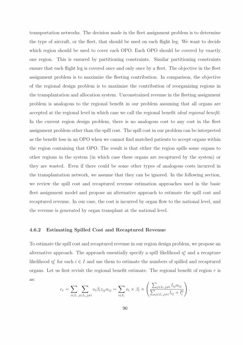
transportation networks. The decision made in the fleet assignment problem is to determine
the type of aircraft, or the fleet, that should be used on each flight leg. We want to decide
which region should be used to cover each OPO. Each OPO should be covered by exactly
one region. This is ensured by partitioning constraints. Similar partitioning constraints
ensure that each flight leg is covered once and only once by a fleet. The objective in the fleet
assignment problem is to maximize the fleeting contribution. In comparison, the objective
of the regional design problem is to maximize the contribution of reorganizing regions in
the transplantation and allocation system. Unconstrained revenue in the fleeting assignment
problem is analogous to the regional benefit in our problem assuming that all organs are
accepted at the regional level in which case we call the regional benefit ideal regional benefit.
In the current region design problem, there is no analogous cost to any cost in the fleet
assignment problem other than the spill cost. The spill cost in our problem can be interpreted
as the benefit loss in an OPO when we cannot find matched patients to accept organs within
the region containing that OPO. The result is that either the region spills some organs to
other regions in the system (in which case these organs are recaptured by the system) or
they are wasted. Even if there could be some other types of analogous costs incurred in
the transplantation network, we assume that they can be ignored. In the following section,
we review the spill cost and recaptured revenue estimation approaches used in the basic
fleet assignment model and propose an alternative approach to estimate the spill cost and
recaptured revenue. In our case, the cost is incurred by organ flow to the national level, and
the revenue is generated by organ transplant at the national level.
4.6.2 Estimating Spilled Cost and Recaptured Revenue
To estimate the spill cost and recaptured revenue in our region design problem, we propose an
alternative approach. The approach essentially specify a spill likelihood ηsi and a recapture
likelihood ηri for each i ∈ I and use them to estimate the numbers of spilled and recaptured
organs. Let us first revisit the regional benefit estimate. The regional benefit of region r is
as:
cr =∑
i∈Ir
∑
j∈Ir,j 6=i
oiβizijαij =∑
i∈Ir
oi × βi ×
(
∑
j∈Ir,j 6=i lijαij∑
j∈Ir,j 6=i lij + l0i
)
.
90

For an i ∈ Ir, oi ·βi · (∑
j∈Ir,j 6=i zij) is the number of organs that are accepted at the regional
level, and thus oi · βi · (∑
j∈Ir,j 6=i(1 − zij)) the number of organs that are made available at
the national level. Then the number of spilled organs from OPO i is
SOi = oi × βi ×l0i
∑
j∈Ir,j 6=i lij + l0i,
and the number of spilled organs from region r is
SOr =∑
i∈Ir
oi × βi ×l0i
∑
j∈Ir,j 6=i lij + l0i.
Let ηsi = l0i . We call it national spill likelihood. The spill cost incurred in region r, denoted
by csr, is computed as the benefit generated if all spilled organs are distributed inside the
region based on proportion allocation. That is,
csr =
∑
i∈Ir
SOi ·
(
∑
j∈Ir,j 6=i
lijαij∑
k∈Ir,k 6=i lik
)
.
To estimate the number of organs accepted for transplantation at the national level, we make
the following assumption.
(A4.4) For organ recapture, the likelihood that an organ procured at one OPO is accepted
at the national level, is proportional to the likelihood of organ distribution to recipient
OPOs that are not included in the same region, when there is only a single national
waiting list.
Note that the only difference between Assumption A4.4 and Assumption A4.2 is that we
only consider the likelihood of national-level organ acceptance in Assumption A4.4. With
the assumption, we further divide national-level flow into two parts, organs that are accepted
and wasted at the national level. Under the condition where there is a single national waiting
list, we call the likelihood of organ acceptance at all recipient OPOs that are not included
91
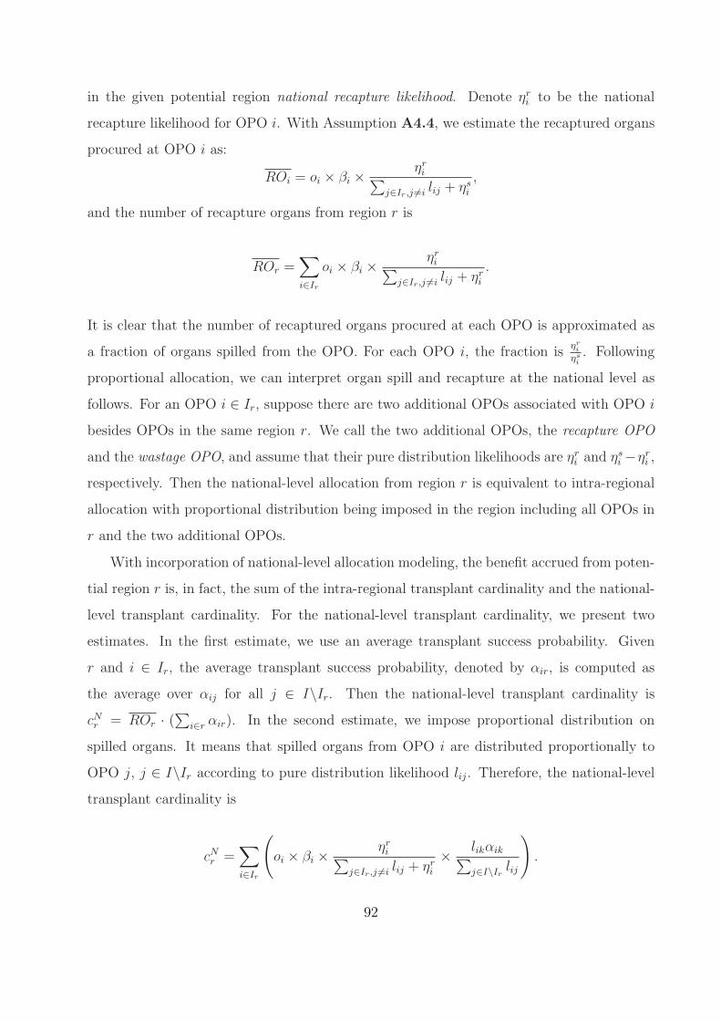
in the given potential region national recapture likelihood. Denote ηri to be the national
recapture likelihood for OPO i. With Assumption A4.4, we estimate the recaptured organs
procured at OPO i as:
ROi = oi × βi ×ηr
i∑
j∈Ir,j 6=i lij + ηsi
,
and the number of recapture organs from region r is
ROr =∑
i∈Ir
oi × βi ×ηr
i∑
j∈Ir,j 6=i lij + ηri
.
It is clear that the number of recaptured organs procured at each OPO is approximated as
a fraction of organs spilled from the OPO. For each OPO i, the fraction isηr
i
ηsi. Following
proportional allocation, we can interpret organ spill and recapture at the national level as
follows. For an OPO i ∈ Ir, suppose there are two additional OPOs associated with OPO i
besides OPOs in the same region r. We call the two additional OPOs, the recapture OPO
and the wastage OPO, and assume that their pure distribution likelihoods are ηri and ηs
i −ηri ,
respectively. Then the national-level allocation from region r is equivalent to intra-regional
allocation with proportional distribution being imposed in the region including all OPOs in
r and the two additional OPOs.
With incorporation of national-level allocation modeling, the benefit accrued from poten-
tial region r is, in fact, the sum of the intra-regional transplant cardinality and the national-
level transplant cardinality. For the national-level transplant cardinality, we present two
estimates. In the first estimate, we use an average transplant success probability. Given
r and i ∈ Ir, the average transplant success probability, denoted by αir, is computed as
the average over αij for all j ∈ I\Ir. Then the national-level transplant cardinality is
cNr = ROr · (
∑
i∈r αir). In the second estimate, we impose proportional distribution on
spilled organs. It means that spilled organs from OPO i are distributed proportionally to
OPO j, j ∈ I\Ir according to pure distribution likelihood lij. Therefore, the national-level
transplant cardinality is
cNr =
∑
i∈Ir
(
oi × βi ×ηr
i∑
j∈Ir,j 6=i lij + ηri
×likαik
∑
j∈I\Irlij
)
.
92

To differentiate intra-regional transplant cardinality in region r and overall transplant cardi-
nality at both regional and national levels, we use cRr to represent the former cardinality and
cr to represent the latter. Then the overall benefit generated by region r through regional-
level and national-level allocation is cr = cRr + cN
r .
At the end of this section, we discuss generalization of the spill likelihood ηsi and the
recapture likelihood ηri . It is more realistic to assume that ηs
i and ηri are dependent upon
the potential region that contains r. Therefore, we can replace ηsi and ηr
i with ηsi,r and
ηri,r, respectively. This generalization does not affect the applicability of the set-partitioning
problem. In fact, in most basic fleeting assignment models, the decision variables are binary
variables indicating whether a flight leg is assigned to a fleet type. It is straightforward to
change our set-partitioning formulation (see Formulation (3.1) in Chapter 3.2) to a formula-
tion in which decision variables are indexed by both OPO and region. One reason of using ηsi
and ηri instead of ηs
i,r and ηri,r is for the applicability of our branch-and-price solution, which
will be discussed in Chapter 5. This is also the reason why we make Assumption A4.3. The
other reason is due to the fact that we estimate the likelihoods using the simulation. More
discussion regarding this reason will be provided in the next section.
Using either ηsi and ηr
i or ηsi,r and ηr
i,r in the region design model does not capture
national-level allocation interdependency or network effects. This is because the number of
national-level transplants within each region depends on what other regions are chosen along
with it, thus violating the linearity property of the set-partitioning problem. To see this,
consider a particular region r. The number of transplants at the national level to patients
in r will be large if the other regions are net suppliers of organs at the national level than
if the other regions are net recipients at the national level. As a summary, organs to spill
from one region should be a function of the demands and supplies of other regions. Without
knowing the entire partition of the network, the above spill-and-recapture estimation step is
inexact.
93

4.6.3 Estimating Spill and Recapture Likelihoods with the Simulation
To estimate the spill likelihood ηsi and recapture likelihood ηr
i , we use the simulation model
LASM. Before presenting our estimation, we review two spill and recapture estimation ap-
proaches used in the basic fleet assignment problem. These two approaches can be found in
[23].
As described earlier, spill costs in the basic fleet assignment model are estimated for each
flight leg and each possible fleet assignment to that leg. There are two major approaches to
spill estimation. The first approach is a deterministic approach that determines the spill for
each flight leg based on its capacity, which is independent of other flight legs. It begins by
listing the passengers in the order of decreasing revenue contribution and then offering seats
to those on the list, in order, until all passengers are processed or capacity is fully utilized.
Lower ranked passengers are spilled and the total revenue of these spilled passengers is the
estimated spill cost for flight leg i. The second spill estimation approach is a probabilistic
approach that the expected spill cost of assigning fleet type k to leg i is computed as the
product of average spill fare, SFk,i, and expected number of spilled passengers, E[tk,i]. The
expected number of spilled passengers, E[tk,i] is estimated by assuming that the flight leg
level demand follows a Gaussian distribution with mean Qi, the average number of passengers
traveling on flight leg i, and standard deviation K ×Qi, where K is between 0.2 and 0.5, or
Z ×√
(Qi), where Z is between 1.0 and 2.5. The details of these estimates can be found in
Kniker [122].
Recaptured revenue is the portion of the spill costs that are recovered by transporting
passengers on itineraries other than their desired itineraries. If spill is only approximated as
in basic fleeting assignment models, then recapture is at best approximate.
Earlier in Section 4.3, we describe the procedure of estimating the pure national flow
likelihood. It is, in fact, the procedure of estimating ηsi . To estimate ηr
i , we follow the same
procedure. In the simulation model, we set the matching algorithm to be such that certain
regional preference is imposed and record every organ that is identified to be made available
and every one that is wasted at the national level, respectively. For a given regional
94

configuration, a number of replications will be run to guarantee the conclusion to be drawn
is of statistical significance. A number of regional configurations are sampled randomly, and
ηsi and ηr
i are point estimates over the sample for each OPO i ∈ I.
Now let us compare our estimation approach with the two approaches used in the basic
fleeting assignment model. Similar to those two approaches, our estimate for each OPO
is independent of other OPOs. Organs are spilled and recaptured based on whether or
not donor-recipient matching exists, which is determined in the simulation model. The
simulation model lists patients in the order of decreasing medical urgency and donor-recipient
compatibility and considers patient autonomy on organ acceptance/rejection. Then it offers
organs to other on the list in order. To some extend, this is similar to considering the
capacity according to the passenger ranking in the above deterministic approach. In our
estimation, we compute the point estimates of ηsi and ηr
i , which is similar to the expected
number of spilled passengers, estimated in the above probabilistic approach.
4.7 SUMMARY OF ASSUMPTIONS
At the end of this chapter, we list all necessary modeling assumptions in the presented
modeling framework and demonstrate the current state of modeling efficiency improvement
of the organ transplant and allocation system through region reorganization.
1. Organ procurement and patient listing are aggregated over transplant centers within
each OPO. (Assumption A3.1)
2. The allocation process is in steady state. (Assumption A3.3)
3. For intra-regional transplantation, the likelihood that an organ procured at one OPO is
accepted by a patient at each other OPO within the same potential region, is proportional
to the likelihood of organ distribution from the donor OPO to a recipient OPO that is in
the same region, where there is only a single national waiting list. (Assumption A4.1)
95

4. For organ flow to the national level, the likelihood that an organ procured at one OPO
is not accepted or wasted at the regional level (and thus made available at the national
level), is proportional to the likelihood of organ distribution to recipient OPOs that are
not included in the same region and organ wastage, when there is only a single national
waiting list. (Assumption A4.2)
5. Given any potential region design, the likelihood that an organ procured at one OPO
is not accepted or wasted at the regional level (and thus made available at the national
level), depends only upon the donor OPO. (Assumption A4.3)
6. For organ recapture, the likelihood that an organ procured at one OPO is accepted at the
national level, is proportional to the likelihood of organ distribution to recipient OPOs
that are not included in the same region, when there is only a single national waiting
list. (Assumption A4.4)
Assumption A3.1 assumes all transplant centers within an OPO service area are ag-
gregated. From the methodological point of view, the modeling framework can be easily
extended to consider improving system efficiency through regrouping transplant centers.
Due to political and administrative reasons, it is, however, unlikely that transplant centers
will be free to choose what other transplant centers are preferable to group with in terms
of allocation efficiency. Assumption A3.3 allows us to study the long-term expected system
performance. It is critical to the applicability of the presented deterministic integer pro-
gramming modeling framework. It also leads the way for us to make assumptions on how
organs are allocated with a macro viewpoint. Relaxing this assumption would allow us to
address system dynamics and uncertainty when estimating the regional benefit but many
additional modeling challenges would surface. Assumptions A4.1 - A4.2 are proportional
allocation assumptions. They are the core assumptions in this dissertation. Assumption
A4.3 is primarily made to ensure the applicability of our branch-and-price solution. It does
not effect the modeling framework. Therefore, the solution through explicit region enumera-
tion would still be valid even if this assumption is relaxed. Assumption A4.4 is an additional
proportional allocation assumption for national-level allocation modeling.
96

5.0 A BRANCH-AND-PRICE APPROACH TO OPTIMAL REGION
DESIGN SOLUTION
As shown in Chapter 4, solving the organ region design problem has presented a great chal-
lenge. An important characteristic of these problems is that each of them has an enormous
number of decision variables, all of which are required to be integral. Due to this, we con-
sider a branch-and-price approach with which we adaptively generate potential regions and
apply a specialized branching rule to balance the search tree. In branch and price, sets of
columns are left out of the LP relaxation because there are too many columns to handle
explicitly and most of them will have their associated variables equal to zero in an optimal
solution anyway. By applying column generation, only “promising” columns are included
in the restricted LP master problem. In our region design problem, each column represents
a potential region. As a result, we iteratively solve the LP master problem of manageable
size. To check the optimality of an LP solution, a subproblem, called the pricing problem,
which is a separation problem for the dual LP, is solved to try to identify columns to enter
the basis. Therefore, in each iteration, we also solve one or many MIP pricing problems to
generate one or many “promising” columns. Once the LP relaxation of the problem over
a set of generated columns is solved, a fractional solution may be obtained. Therefore,
branching is required. It occurs when no columns price out favorably to enter the basis and
the LP solution does not satisfy some integrality condition. A commonly used branching
rule is branching on variables. Many computational studies, however, have shown that it
does not perform well in set-partitioning instances due to an resulting unbalanced search
tree. Therefore, we consider application of a specialized branching rule for our region design
problem.
97
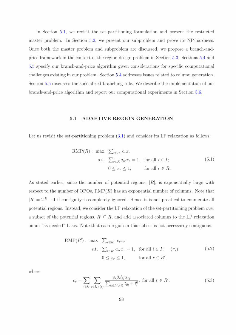
In Section 5.1, we revisit the set-partitioning formulation and present the restricted
master problem. In Section 5.2, we present our subproblem and prove its NP-hardness.
Once both the master problem and subproblem are discussed, we propose a branch-and-
price framework in the context of the region design problem in Section 5.3. Sections 5.4 and
5.5 specify our branch-and-price algorithm given considerations for specific computational
challenges existing in our problem. Section 5.4 addresses issues related to column generation.
Section 5.5 discusses the specialized branching rule. We describe the implementation of our
branch-and-price algorithm and report our computational experiments in Section 5.6.
5.1 ADAPTIVE REGION GENERATION
Let us revisit the set-partitioning problem (3.1) and consider its LP relaxation as follows:
RMP(R) : max∑
r∈R crxr
s.t.∑
r∈R airxr = 1, for all i ∈ I;
0 ≤ xr ≤ 1, for all r ∈ R.
(5.1)
As stated earlier, since the number of potential regions, |R|, is exponentially large with
respect to the number of OPOs, RMP(R) has an exponential number of columns. Note that
|R| = 2|I| − 1 if contiguity is completely ignored. Hence it is not practical to enumerate all
potential regions. Instead, we consider the LP relaxation of the set-partitioning problem over
a subset of the potential regions, R′ ⊆ R, and add associated columns to the LP relaxation
on an “as needed” basis. Note that each region in this subset is not necessarily contiguous.
RMP(R′) : max∑
r∈R′ crxr
s.t.∑
r∈R′ airxr = 1, for all i ∈ I; (πi)
0 ≤ xr ≤ 1, for all r ∈ R′,
(5.2)
where
cr =∑
i∈Ir
∑
j∈Ir\{i}
oiβilijαij∑
k∈Ir\{i} lik + l0i, for all r ∈ R′. (5.3)
98

Such a linear relaxation is called a “restricted master problem” in the context of column
generation. We assign an optimal dual variable, denoted by πi, to each set-partitioning
constraint in RMP(R′) (see Problem 5.2) corresponding to OPO i. Given a potential region
r, the reduced cost cr is then as:
cr = cr −∑
i∈I
airπi = cr −∑
i∈Ir
πi. (5.4)
It is clear that an optimal solution to RMP(R′) is a feasible solution to the unrestricted
master problem (LP relaxation of the original set-partitioning problem) RMP(R). To deter-
mine if this feasible solution is optimal to RMP(R), we need to check if there are columns in
R\R′ that price out favorably. This is done by solving the following pricing problem given
the current dual variables π: maxr∈R cr = maxr∈R{cr −∑
i∈Irπi}. Define yi = 1 if i ∈ Ir;
yi = 0, otherwise. Then cr in (5.3) can be rewritten as:
cr =∑
i∈I
[∑
j∈I\{i} oiβiαijlijyj∑
j∈I\{i} lijyj + l0i yi
]
· yi.
Consequently, the pricing problem is rewritten as:
RPP(π) : max∑
i∈I
[∑
j∈I\{i} oiβiαijlijyj∑
j∈I\{i} lijyj + l0i yi
]
· yi −∑
i∈I
πiyi (5.5)
subject to
yi ∈ {0, 1}, for all i ∈ I. (5.6)
If the optimal objective value is less than or equal to 0, then an optimal solution to
RMP(R) is found. Otherwise, a new column is generated as follows. An OPO i is included
in the newly generated region if and only if yi = 1.
RPP may be formulated as an unconstrained nonlinear pure 0-1 program. To be more
specific, its objective function is a pseudo-Boolean function, i.e., f : IB|I| 7→ IR. A standard
procedure of linearizing nonlinear pure 0-1 programs is to represent the pseudo-Boolean
objective function as a posiform, i.e, a polynomial expression in terms of all the literals and
their negations that correspond to decision variables [32]. Unfortunately, in our problem,
the equivalent posiform includes one term for each potential region. Thus, the resulting
problem after the linearization is to pick the decision variable which gives the most favorable
99
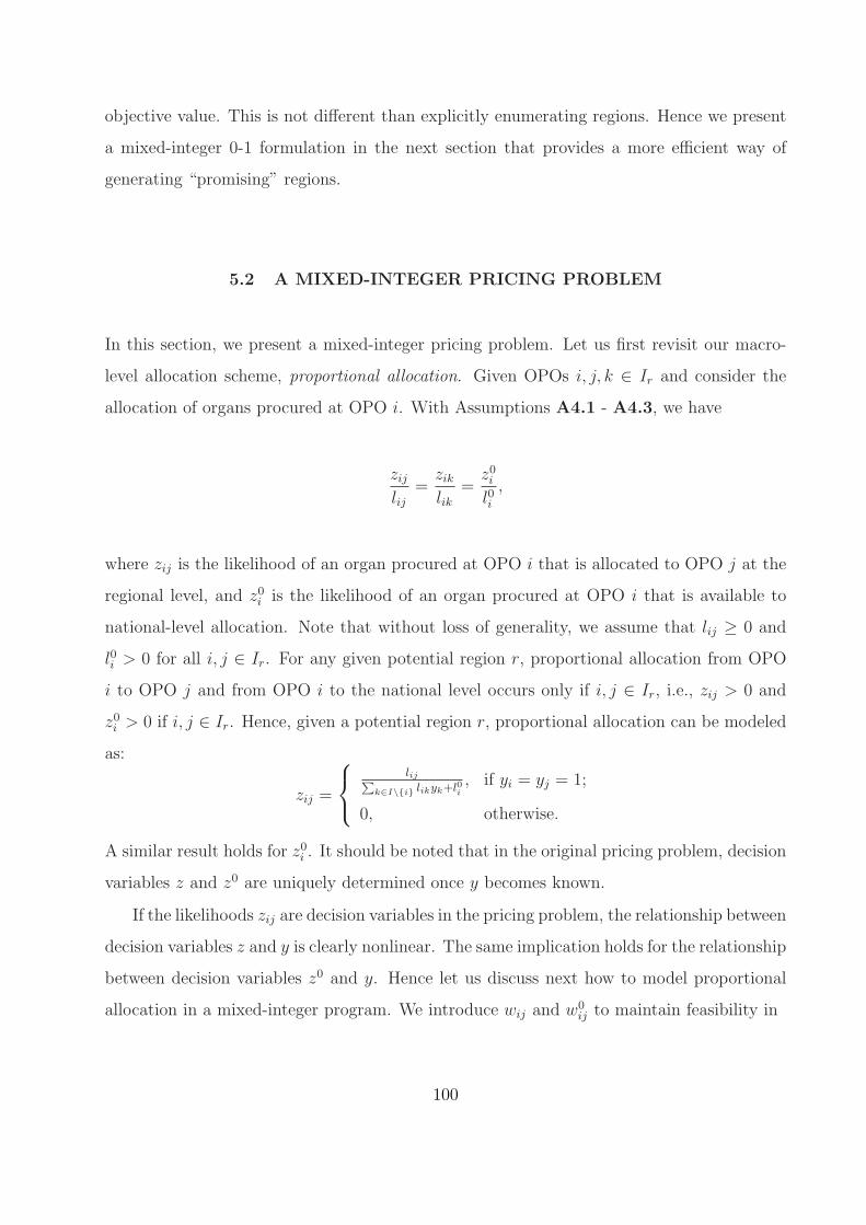
objective value. This is not different than explicitly enumerating regions. Hence we present
a mixed-integer 0-1 formulation in the next section that provides a more efficient way of
generating “promising” regions.
5.2 A MIXED-INTEGER PRICING PROBLEM
In this section, we present a mixed-integer pricing problem. Let us first revisit our macro-
level allocation scheme, proportional allocation. Given OPOs i, j, k ∈ Ir and consider the
allocation of organs procured at OPO i. With Assumptions A4.1 - A4.3, we have
zij
lij=
zik
lik=
z0i
l0i,
where zij is the likelihood of an organ procured at OPO i that is allocated to OPO j at the
regional level, and z0i is the likelihood of an organ procured at OPO i that is available to
national-level allocation. Note that without loss of generality, we assume that lij ≥ 0 and
l0i > 0 for all i, j ∈ Ir. For any given potential region r, proportional allocation from OPO
i to OPO j and from OPO i to the national level occurs only if i, j ∈ Ir, i.e., zij > 0 and
z0i > 0 if i, j ∈ Ir. Hence, given a potential region r, proportional allocation can be modeled
as:
zij =
lijP
k∈I\{i} likyk+l0i, if yi = yj = 1;
0, otherwise.
A similar result holds for z0i . It should be noted that in the original pricing problem, decision
variables z and z0 are uniquely determined once y becomes known.
If the likelihoods zij are decision variables in the pricing problem, the relationship between
decision variables z and y is clearly nonlinear. The same implication holds for the relationship
between decision variables z0 and y. Hence let us discuss next how to model proportional
allocation in a mixed-integer program. We introduce wij and w0ij to maintain feasibility in
100

the mixed-integer pricing problem. Given that OPO i is included in the selected potential
region r, if two other OPOs j and k are also included in r, the proportional allocation
between j and k must be enforced. That is,
likzij ≤ lijzik + likwjk; (5.7)
lijzik ≤ likzij + lijwjk; (5.8)
wjk ≤ 2− yj − yk. (5.9)
Similarly, we develop the proportionality constraints between organ distribution to an OPO
at the regional level and that to the national level as follows:
lijz0i ≤ l0i zij + lijw
0ji; (5.10)
l0i zij ≤ lijz0i + l0i w
0ji; (5.11)
w0ji ≤ 2− yj − yi. (5.12)
Note that decision variables zij and zi0, for all i, j ∈ I, are continuous variables bounded
between 0 and 1 since they measure the allocation likelihood. Note also that decision vari-
ables wij and w0ij, for all i, j ∈ I, are also continuous variables bounded between 0 and 1. If
both OPOs j and k are included in the selected potential region r, Inequality (5.9) implies
wjk = 0 and thus Inequalities (5.7) and (5.8) are satisfied with equality. Hence, proportional
allocation of organs procured at OPO i to OPOs j and k is enforced. If one or both OPOs
are not selected, Inequality (5.9) is not tight and thus Inequalities (5.7) - (5.8) do not impose
any additional restriction on zij and zik. A similar implication can be seen in Inequalities
(5.10) - (5.12).
Next we present the pricing problem as:
RPP MIP(π) : max∑
i∈I
∑
j∈I\{i}oiβiαijzij −
∑
i∈I
πiyi (5.13)
subject to∑
j∈I\{i}zij + z0
i = yi,∀i ∈ I; (5.14)
zij ≤ yj,∀i, j ∈ I, i 6= j; (5.15)
101

likzij ≤ lijzik + likwjk,∀i, j, k ∈ I, i 6= j, k, j < k; (5.16)
lijzik ≤ likzij + lijwjk,∀i, j, k ∈ I, i 6= j, k, j < k; (5.17)
wjk ≤ 2− yj − yk,∀j, k ∈ I, j < k; (5.18)
l0i zij ≤ lijz0i + likw
0ji,∀i, j ∈ I, i 6= j; (5.19)
lijz0i ≤ l0i zij + lijw
0ji,∀i, j ∈ I, i 6= j; (5.20)
w0ji ≤ 2− yj − yi,∀i, j ∈ I, i 6= j; (5.21)
yi ∈ IB, 0 ≤ z0i ≤ 1,∀i ∈ I; 0 ≤ wij ≤ 1,∀i, j ∈ I, i < j; (5.22)
0 ≤ zij, w0ij ≤ 1,∀i, j ∈ I, i 6= j. (5.23)
The objective function (5.13) is equivalent to (5.5), the objective function of RPP(π).
Constraints (5.14) ensure that organs procured at OPO i are allocated at the regional level
only if OPO i is included in the selected region. Constraints (5.15) ensure that organs
procured at OPO i are allocated to OPO j only if OPO j is included in the selected region.
For an OPO i in the selected region r, if both OPOs j and k are also included in r,
yj = yk = 1, Constraints (5.16) - (5.18) enforce proportional allocation between i to j and
i to k. Hence, we call these constraints proportionality constraints. If OPO j is included
and OPO k is excluded in r, yk = 0, and thus zik = 0 by Constraint (5.15). Similarly, we
know zij = zik = 0 if neither OPO is included in r, i.e., yj = yk = 0. Therefore, given
any OPO i ∈ Ir, we enforce proportional allocation on any other two OPOs j, k ∈ Ir. Note
that by introducing additional decision variables, we model proportional allocation with
linear constraints. In the same manner, given any OPO i in the selected region r, we model
proportional allocation between any other OPO j ∈ Ir and the national level, as shown in
Constraints (5.19) - (5.21). In these constraints, decision variables w0ij, similar to wij, are
introduced to maintain feasibility in RPP MIP.
To summarize, the first class of proportionality constraints enforces proportional alloca-
tion between OPOs and the second class enforces proportional allocation between an OPO
102

and the national level. Note that the mixed-integer pricing problem (5.13) - (5.23) can be
simplified by combining similar decision variables and replacing variables with their com-
plements. Therefore, various mixed-integer programming formulations are derived. We will
study several alternative formulations in the next chapter.
A characteristic of this pricing problem is that if proportionality constraints are relaxed,
the problem is similar to a facility location problem where each variable yj indicates whether
location j should be selected to build a warehouse and each variable zij indicates what pro-
portion of the commodity in the warehouse at location j should be shipped to the customer
at location i. However, the decision at the operational level is fixed after knowing the deci-
sion at the strategic level due to the proportional allocation requirement, i.e., if y variables
are determined, z variables are uniquely determined due to proportional allocation.
Some pricing problems arising in integer programming column generation, such as the
shortest path pricing problem for the multi-commodity flow problem and the integer knap-
sack pricing problem for the cutting stock problem, are easy to solve practically and/or
theoretically. For example, when applying column generation to the multi-commodity flow
problem, the pricing problem is a shortest path problem that possesses the integrality prop-
erty. In other words, the pricing problem is polynomial solvable. The integrality property
means that the convex hull of the feasible solution set of the pricing problem is an integral
polyhedron. Hence its natural formulation gives integral optimal solutions. When applying
column generation to the cutting stock problem, the pricing problem is an integer knapsack
problem whose LP relaxation can be strengthened. Although the integer knapsack problem is
NP-hard, there are exact pseudo-polynomial algorithms in practice. Other column generation
applications where the pricing problem is easy to solve, include graph partitioning problems
[62, 149] (e.g., minimum cut clustering [119, 212]), bin packing problems [205, 206], and the
multi-item lot-sizing problem [212]. Although the maximum weighted independent set prob-
lem, the pricing problems for graph coloring problems [151], is NP-hard, the problem is well
studied in graph theory and combinatorial optimization, and various solution approaches
have been tried. Column generation applications to many vehicle routing and crew schedul-
ing problems have the structure that the master problem results in set-partitioning/covering
type problems and the subproblem is strongly NP-hard (see Barnhart et al. [18], Desaulniers
103
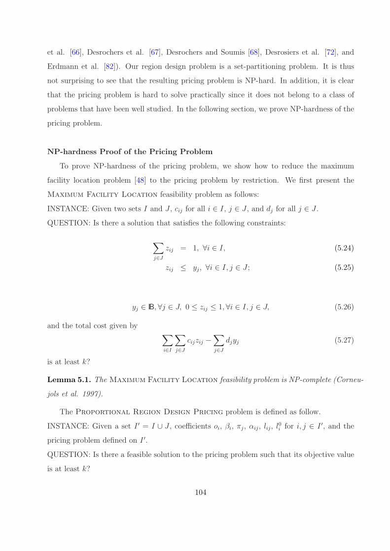
et al. [66], Desrochers et al. [67], Desrochers and Soumis [68], Desrosiers et al. [72], and
Erdmann et al. [82]). Our region design problem is a set-partitioning problem. It is thus
not surprising to see that the resulting pricing problem is NP-hard. In addition, it is clear
that the pricing problem is hard to solve practically since it does not belong to a class of
problems that have been well studied. In the following section, we prove NP-hardness of the
pricing problem.
NP-hardness Proof of the Pricing Problem
To prove NP-hardness of the pricing problem, we show how to reduce the maximum
facility location problem [48] to the pricing problem by restriction. We first present the
Maximum Facility Location feasibility problem as follows:
INSTANCE: Given two sets I and J , cij for all i ∈ I, j ∈ J , and dj for all j ∈ J .
QUESTION: Is there a solution that satisfies the following constraints:
∑
j∈J
zij = 1, ∀i ∈ I, (5.24)
zij ≤ yj, ∀i ∈ I, j ∈ J ; (5.25)
yj ∈ IB,∀j ∈ J, 0 ≤ zij ≤ 1,∀i ∈ I, j ∈ J, (5.26)
and the total cost given by∑
i∈I
∑
j∈J
cijzij −∑
j∈J
djyj (5.27)
is at least k?
Lemma 5.1. The Maximum Facility Location feasibility problem is NP-complete (Corneu-
jols et al. 1997).
The Proportional Region Design Pricing problem is defined as follow.
INSTANCE: Given a set I ′ = I ∪ J , coefficients oi, βi, πj, αij, lij, l0i for i, j ∈ I ′, and the
pricing problem defined on I ′.
QUESTION: Is there a feasible solution to the pricing problem such that its objective value
is at least k?
104
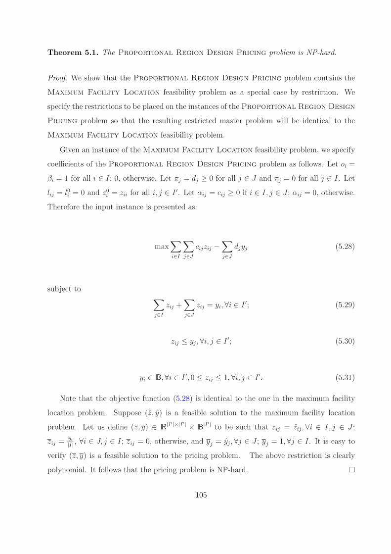
Theorem 5.1. The Proportional Region Design Pricing problem is NP-hard.
Proof. We show that the Proportional Region Design Pricing problem contains the
Maximum Facility Location feasibility problem as a special case by restriction. We
specify the restrictions to be placed on the instances of the Proportional Region Design
Pricing problem so that the resulting restricted master problem will be identical to the
Maximum Facility Location feasibility problem.
Given an instance of the Maximum Facility Location feasibility problem, we specify
coefficients of the Proportional Region Design Pricing problem as follows. Let oi =
βi = 1 for all i ∈ I; 0, otherwise. Let πj = dj ≥ 0 for all j ∈ J and πj = 0 for all j ∈ I. Let
lij = l0i = 0 and z0i = zii for all i, j ∈ I ′. Let αij = cij ≥ 0 if i ∈ I, j ∈ J ; αij = 0, otherwise.
Therefore the input instance is presented as:
max∑
i∈I
∑
j∈J
cijzij −∑
j∈J
djyj (5.28)
subject to∑
j∈I
zij +∑
j∈J
zij = yi,∀i ∈ I ′; (5.29)
zij ≤ yj,∀i, j ∈ I ′; (5.30)
yi ∈ IB,∀i ∈ I ′, 0 ≤ zij ≤ 1,∀i, j ∈ I ′. (5.31)
Note that the objective function (5.28) is identical to the one in the maximum facility
location problem. Suppose (z, y) is a feasible solution to the maximum facility location
problem. Let us define (z, y) ∈ IR|I′|×|I′| × IB
|I′| to be such that zij = zij,∀i ∈ I, j ∈ J ;
zij = yi
|I| , ∀i ∈ J, j ∈ I; zij = 0, otherwise, and yj = yj,∀j ∈ J ; yj = 1,∀j ∈ I. It is easy to
verify (z, y) is a feasible solution to the pricing problem. The above restriction is clearly
polynomial. It follows that the pricing problem is NP-hard.
105

5.3 A BRANCH-AND-PRICE ALGORITHMIC FRAMEWORK
In this section, we present an overview of our branch-and-price algorithmic framework. Sev-
eral relevant topics will be discussed with more details in later sections.
As discussed in Chapter 2, branch and price involves combining well known ideas of
applying column generation to large-scale linear programs and applying branch and bound
to integer programs. First, let us discuss our application of branch and bound. A branch-
and-bound algorithm [155] partitions the solution space into subproblems and then optimizes
individually over each subproblem. Using branch and bound, we initially examine the entire
solution space S and seek a feasible solution s ∈ S. In the bounding phase, we relax the
problem. In so doing, we admit solutions that are not necessarily integer feasible. Solving
this relaxation yields an upper bound on the value of an optimal solution. If the solution
to this relaxation is integer feasible, we are done. Otherwise, we identify n subsets S1, . . . ,
Sn of S, such that ∪ni=1Si = S. Each of these subsets is called a subproblem; S1, . . . , Sn are
sometimes called the children of S. We add S1, . . . , Sn to the list of candidate subproblems.
This is called branching. In our case, these subsets S1, . . . , Sn are subsets of potential regions
with some restrictions modeling relationships between OPOs.
To continue the algorithm, we select one of the candidate subproblems and process it.
There are four possible results. If we find a feasible solution better than s, then we replace s
with the new solution and continue. We may also find that the subproblem has no solutions,
in which case we prune it. Otherwise, we compare the upper bound for the subproblem to our
global lower bound, given by the value of the best feasible solution found so far. If it is less
than or equal to our current lower bound, then we may again prune the subproblem. Finally,
if we cannot prune the subproblem, we are forced to branch and add the children of this
subproblem to the list of active candidates. We continue this way until the list of candidate
subproblems is empty, at which point our current best solution is, in fact, optimal. The
general branch-and-bound algorithmic procedure is also reviewed in the following flowchart
(see Figure 22), where glb and lub represent the global lower bound and local upper bound
for a considered subproblem, respectively.
106

Figure 22: Branch-and-Bound Algorithm
107

Figure 23: Illustration of Branch and Price
Next we discuss our application of column generation. Each subproblem encountered
throughout the branch-and-bound solution can be represented as a node in a search tree.
In our application, the bounding operation is accomplished by using the tools of linear
programming [108]. In other words, at each node of the branch-and-bound tree, an LP
solution is required. Therefore, our algorithm is an LP-based branch-and-price algorithm.
In our large-scale set-partitioning problem, solving such LP relaxations of subproblems with
an enormous number of columns becomes one of the bottlenecks. However, some of the
columns (decision variables and their corresponding constraint matrix coefficients) can be
defined implicitly. Let the set of the columns be R. If column r ∈ R is not present in the
current constraint matrix, then variable xr is implicitly taken to have value zero. Pricing
is necessary before a search tree node can be fathomed. Its purpose is to check if the LP-
solution computed over a subset of decision variables R′ ⊂ R is valid for R, i.e., all non-active
variables “price out” correctly. The process of dynamically generating variables is called
pricing. Hence, our proposed LP-based branch-and-bound algorithm in which variables are
generated dynamically is known as a branch-and-price algorithm (see Figure 23).
108

Before presenting the algorithmic framework, we introduce some notation used in the
presentation. Let F(SR′) be the feasible solution set of subproblem SR′ given that R′ is the
set of considered decision variables. Then the feasible set of RMP(R), the LP relaxation
of the original set-partitioning problem, is represented by F(SIR), where SI is the initial
subproblem, the problem at the root node of the search tree. For a review of the general
branch-and-price algorithm, we refer to Vance [208].
Algorithm 5.1. (A Branch-and-Price Algorithm)
Input: An optimal region design problem instance.
Output: An optimal solution x∗ and its corresponding optimal regional configuration R∗ to
the problem instance.
Step 1. Generate a “good” feasible solution x corresponding to regional configuration R.
Set α←∑
r∈R cr.
Step 2. Generate the initial subproblem SIR′ by constructing R ⊆ R′ ⊂ R, a small set of
potential regions. Set B ← {SIR′} and L′ ← ∅.
Step 3. If B = ∅, STOP and output x as the global optimum x∗ and R as the optimal
configuration R∗. Otherwise, choose some S ∈ B. Set B ← B\{S}. Apply the bounding
operation to S (see Algorithm 5.2).
Step 4. If the result of Step 3 is a feasible solution x corresponding to regional configuration
R and∑
r∈R cr >∑
r∈R cr. Set R ← R and α ←∑
r∈R cr and go to Step 3. If the
subproblem was pruned, go to Step 3. Otherwise, go to Step 5.
Step 5. Perform the branching operation (see Algorithm 5.3). Add the set of generated
subproblems to B and go to Step 3.
Algorithm 5.2. (Bounding Operation)
Input: A subproblem S, described in terms of a subset of potential regions, R′ ⊆ R and a set
of additional constraints L′ modeling relationships between OPOs such that F(SR′) = {x ∈
IR|R′|+ :
∑
r∈R′ airxr = 1,∀i ∈ I, ax ≤ β, (a, β) ∈ L′} and α, an lower bound on the optimal
objective value.
109
Output: Either (1) an integer optimal solution x to the subproblem S, (2) an upper bound
on the optimal value of the subproblem and the corresponding relaxed solution xLP , or (3) a
message pruned indicating that the subproblem should not be considered further.
Step 1. If F(SR) = ∅, then STOP and output pruned. This subproblem has no feasible
solutions.
Step 2. Otherwise, construct the initial feasible set of columns R such that R′ ⊆ R and
F(SR) 6= ∅.
Step 3. Solve the LP max{∑
r∈R crxr |∑
r∈R airxr = 1,∀i ∈ I; ax ≤ β, (a, β) ∈ L′; xr ≥
0,∀r ∈ R} and obtain the primal solution x and dual solution π.
Step 4. Apply heuristics and separation algorithms to π, i.e., solve RPP(π) given a set of
constraints on y variables corresponding to L′, to obtain a set of new columns R′ that price
out favorably. If R′ 6= ∅, set R← R ∪ R′ and go to Step 3.
Step 5. Otherwise, x is an optimal solution to S. If x ∈ IB|R|+ , let R be the corresponding
regional configuration and go to Step 6. Otherwise, go to Step 7.
Step 6. If∑
r∈R cr > α, STOP and output x. Otherwise, STOP and output pruned.
Step 7. If∑
r∈R crxr > α, set xLP ← x. STOP and output xLP . Otherwise, STOP and
output pruned.
Algorithm 5.3. (Branching Operation)
Input: A subproblem S, described in terms of a subset of potential regions, R′ ⊆ R, and
x′ ∈ F(SR′), the LP solution yielding the upper bound.
Output: S1,S2, two children subproblems of S.
Step 1: Determine sets L1 and L2 of inequalities such that ∩2i=1{x ∈ F(SR′) : ax ≤
β,∀(a, β) ∈ Li} = ∅ and x′ /∈ ∪2i=1{x ∈ F(SR′) : ax ≤ β,∀(a, β) ∈ Li},
Step 2: Set F(S iR′) = {x ∈ IR
|R′|+ :
∑
r∈R′ airxr = 1,∀i ∈ I; ax ≤ β,∀(a, β) ∈ Li ∪L′}, where
L′ is the set of additional inequalities used to describe S.
The above presentation is a generic framework of the branch-and-price application to
the optimal region design problem. We will next discuss a few specific considerations in our
application. To start any column generation scheme, an initial restricted master problem
has to be provided. In our problem, the basis formed by regions with a single OPO is
110

already feasible. Therefore, an easily constructed initial restricted master problem contains
|I| columns, each of which has objective coefficient ci = 0 and unit vector ar = ei in the initial
constraint matrix. In this way, we can easily ensure the existence of an initial feasible basis
in constructing the restricted master problem. However, since the initial restricted master
problem determines the initial dual variables that will be passed to the pricing problem, a
“good” initial restricted master problem can be important. Two alternatives in initialization
of our column generation are to generate a subset of regions a priori and to generate a pre-
determined regional configuration. For the first alternative, an easy approach is to generate
all contiguous regions that only contain a few OPOs. It is easy to ensure the existence of a
feasible LP-relaxation when generating a large enough set of columns. More importantly, a
large set of initial columns would presumably lead to “good” initial dual variables. However,
generating a large set may be quite time-consuming. Hence, a trade-off is presented in terms
of the number of initially generated columns. For the second alternative, an easy approach is
to use the current regional configuration to construct the initial restricted master problem.
To get a warm start, we can also use some optimal configuration obtained from solving the
region design problem through explicit region enumeration as described in Chapter 4. In
Section 5.6.3, we will discuss with more details the initialization issue in our problem based
on our computational experiments. To summarize, it is straightforward to guarantee the
existence of an initial feasible basis in our problem. However, it is challenging to obtain a
“good” initial feasible basis.
The most computationally intensive component of our branch-and-price algorithm is
solving the pricing problem. Given this fact, we develop our pricing scheme and pricing
problem solution strategies to alleviate this computational bottleneck. We will then elaborate
Steps 3 and 4 of Algorithm 5.2 in our branch-and-price application as follows.
In the pricing problem, we are free to choose a subset of non-basic variables, and a cri-
terion according to which column is selected from the chosen set. According to the classic
largest-coefficient rule [52], one chooses among all columns the one with the most nega-
tive reduced cost (for a minimization problem). However, Sol [193] showed that not using
the largest-coefficient method rule may be theoretically advantageous for set-partitioning
restricted master problems. Our pricing scheme is to generate a set of feasible columns en-
111

countered in the pricing problem solution process. In one extreme case, this set of feasible
columns may just contain the optimal solution. Then our scheme is equivalent to the largest-
coefficient rule. In the other extreme case, this set contains all feasible columns encountered
in the pricing problem solution. Given the fact that our pricing problem is hard to solve,
generating only one column from the solution may not be effective. Our consideration here
is to utilize the dual information provided by multiple columns that are potentially opti-
mal or near optimal. Some alternative pricing rules in the literature include lambda pricing
[29],steepest-edge pricing [90, 101], and dual pendant deepest-cut pricing [212]. Sol [193]
reported that steepest-edge pricing performs particularly well for set-partitioning restricted
master problems.
Therefore the efficiency of column generation hinges on the issue how to price our both
theoretically and practically hard pricing problem efficiently and generate “promising” fea-
sible columns effectively. To address this issue, we develop a decomposition approach that
constructs and solves smaller-scale pricing problems over subsets of the OPO set. This pro-
vides a set of “promising” columns, which coincides with our pricing scheme discussed above
and makes good pricing more achievable. More importantly, these “promising” columns can
be quite distinct since they are generated from various subsets of the OPO set. Along with
our pricing scheme, this approach can be viewed as multiple column generation, a class of
IP column generation acceleration techniques. More details regarding the decomposition
approach are presented in Section 5.4. Many pricing problems in the literature are easy
to solve because either they are well studied or they possess integrality property, i.e., the
convex hull of the feasible solution set of the pricing problem is an integral polyhedron. The
integer knapsack pricing problem of the cutting stock problem falls into the first category
[212] whereas the shortest path pricing problem for the multi-commodity flow problem falls
into the second [98]. Unlike those pricing problems, our problem is not well studied nor pos-
sess the integrality property. We study the polyhedral structure of the problem and develop
several valid inequalities. The polyhedral study is presented in Chapter 6.
At Step 1 of Algorithm 5.3, the branching scheme is presented generically. For large-scale
set-partitioning problems, the branching strategy suggested by Ryan and Foster [181] has
been shown very effective. We adapt their approach and develop a specialized branching
112

scheme. We call our branching scheme branching on OPO pairs. Compared to the standard
branching scheme, branching on variables, this branching scheme results in a more balanced
search tree. We will discuss this scheme in Section 5.5.
Barnhart et al. [22] provided a thorough review of branch-and-price algorithms. For
detailed discussion in the algorithmic aspect of branch and price, we refer to Elf et al.
[79] and Ladanyi et al. [128]. Many selected topics in column generation were covered in
Desrosiers and Lubbecke [71].
5.4 GEOGRAPHIC DECOMPOSITION
In order to alleviate the difficulty in solving our mixed-integer pricing problem, we design
a set of region covers to cover the entire country and construct smaller-scale mixed-integer
pricing problems over these region covers. In the pricing problem, there are O(n3) constraints.
Considering poor scalability of integer programming, our idea here is that we would rather
solve a number of smaller pricing problems. To ensure that we are still capable of identifying
“promising” regions in the column generation, we solve smaller pricing problems over a set
of overlapping region covers as follows.
Figure 24 provides an illustration of geographic decomposition. There are four region
covers specified by blue, light green, and pink lines. We call them the “blue”, “light green”,
“pink”, and “brown” covers, respectively. For example, the “blue” cover contains all OPOs
in the west half of the U.S, and the “brown” cover contains all OPOs in the northeast.
The most important feature of our geographic decomposition is that these designed covers
overlap. In Figure 24, the “blue” and “light green” covers overlap in Minnesota, Iowa,
Nebraska, etc. The “brown” cover overlaps with the “pink” cover in Virginia and overlaps
with the “light green” cover in Northeast Ohio.
113
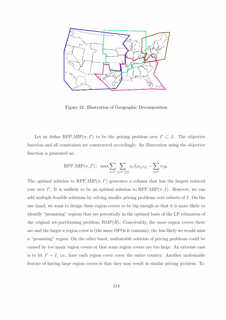
Figure 24: Illustration of Geographic Decomposition
Let us define RPP MIP(π, I ′) to be the pricing problem over I ′ ⊂ I. The objective
function and all constraints are constructed accordingly. An illustration using the objective
function is presented as:
RPP MIP(π, I ′) : max∑
i∈I′
∑
j∈I′\{i}oiβiαijzij −
∑
i∈I′
πiyi.
The optimal solution to RPP MIP(π, I ′) generates a column that has the largest reduced
cost over I ′. It is unlikely to be an optimal solution to RPP MIP(π, I). However, we can
add multiple feasible solutions by solving smaller pricing problems over subsets of I. On the
one hand, we want to design these region covers to be big enough so that it is more likely to
identify “promising” regions that are potentially in the optimal basis of the LP relaxation of
the original set-partitioning problem, RMP(R). Conceivably, the more region covers there
are and the larger a region cover is (the more OPOs it contains), the less likely we would miss
a “promising” region. On the other hand, undesirable solution of pricing problems could be
caused by too many region covers or that some region covers are too large. An extreme case
is to let I ′ = I, i.e., have each region cover cover the entire country. Another undesirable
feature of having large region covers is that they may result in similar pricing problem. To
114

overcome this difficulty, one can apply partial column generation, another IP column gener-
ation acceleration technique, in which not all pricing problems are solved at each iteration
to generate new columns [95].
Given a region covers design I ′, we solve a set of smaller-scale pricing problems RPP MIP(π, I ′)
over I ′i ⊂ I and I ′
i ∈ I′ for all i = 1, . . . , |I ′|. Once no additional columns can price out
favorably with respect to any I ′i, we obtain a feasible solution to RMP(R). Let R′
i be the
set of potential regions given I ′i for all i = 1, . . . , |I ′|. Consider a complete graph G = (I, E)
induced by the set of OPOs I, then R′i is the set of cliques where all nodes are in I ′
i. With
geographic decomposition, we in fact solve the problem RMP(∪|I′|i=1R
′i). Clearly, ∪|I′|
i=1R′i ⊆ R.
Since it is possible that a “promising” region crosses two region covers, this solution is not
provably optimal if we do not check the existence of positive reduced costs in RPP MIP(π, I).
However, proving the optimality of RMP(R) requires us to solve RMP(R) at least once,
which is undesirable. A trade-off is presented between solution time and solution quality
when solving the restricted master problem at each node in the search tree. Next we state
the bounding operation with incorporation of geographic decomposition. Given a region
covers design I ′, we modify Steps 4 and 5 of Algorithm 5.2 as follows.
Alternative Subroutine of Algorithm 5.2 (Incorporating Geographic Decompo-
sition)
Step 4. Apply separation algorithms to π over a subset I ′i ⊂ I and I ′
i ∈ I′ for all
i = 1, . . . , |I ′|, i.e., solve RPP MIP(π, I ′i) given the set of constraints on variables yi, i ∈ I ′,
corresponding to a subset of L′, to obtain a set of new columns R′i,∀i = 1, . . . , |I ′|, that
price out favorably. If R′i = ∅, ∀i, then the incumbent solution x is the optimal solution to
RMP(∪|I′|i=1R
′i) and go to Step 6.
Step 5. Otherwise, set R← R ∪ (∪|I′|i=1R
′i) and go to Step 3.
Step 6. Check if x is also optimal to RMP(R). If not, apply column generation to x
over I, i.e., solve RPP MIP(π).
Note that Step 6 in the above subroutine is optional. This reflects the consideration of the
trade-off stated above. With each region cover, Algorithm 5.2 has more flexibility in terms
of the pricing scheme. We consider generating multiple columns encountered throughout
115

the solution of RPP MIP(π, I ′i). Therefore, with incorporation of geographic decomposition,
our pricing scheme is to generate multiple columns over each region cover in a region covers
design and thus the total number of columns generated at each iteration is∑|I′|
i=1 |R′i|.
From above, we know designing region covers is critical to the efficiency of column gener-
ation and consequently the success of applying branch and price. There are two parameters
to measure a region covers design. One is the number of region covers. The other one is
the size of each region cover. Intuitively, they are two main factors determining the solution
time and quality of the column generation. Poor scalability of integer programming suggests
that the latter is more critical.
Even if two region covers designs have the same number of region covers and the same
number of OPOs in each region cover, they may lead to significantly different solutions in
terms of both the solution quality and solution time. To design good region covers, one may
use regions in the optimal regional configuration obtained through explicit enumeration of
contiguous regions. Besides applying geographic decomposition to alleviate the difficulty in
solving the pricing problem, we explore various column generation strategies with respect
to the number of columns allowed to generate at each iteration. Our considerations are
whether we can prematurely terminate the column generation process at each node and how
important it is to find an optimal solution in solving the pricing problem. In addition, we test
a number of MIP solution parameters used in solving the pricing problem. More discussion
will be presented in Section 5.6 on both the effect of geographic decomposition and other
considerations on the solution of the optimal region design problem. Two rounding heuristic
algorithms are also considered in solving our pricing problem. Solving the LP-relaxation
of the pricing problem RPP MIP(π) provides a LP-relaxation solution, denoted as (y, z).
Let C be the set of dimensions i where yi is fractional. The first heuristic is to round
yi componentwise to the nearest integer for all i ∈ C. If this integer solution prices out
favorably, a new column is added to the restricted master problem accordingly. Otherwise,
we check whether a column that prices out favorably can be generated in the pricing problem
based on other region covers. We terminate column generation at each search tree node when
no integer solution can be found that prices out favorably at the current iteration. Using the
second heuristic, we first compare the reduced costs of neighboring integer solutions to the
116

LP solution on all dimensions in C. Then we select the one with the most positive reduced
cost and add it to the restricted master problem. The heuristic terminates at each search
tree node when no neighboring integer solution yields a positive reduced cost at the current
iteration. Clearly, both heuristics cannot ensure to generate all columns that are needed to
form the optimal basis and thus they do not have finite termination guarantee.
5.5 BRANCHING ON OPO PAIRS
An LP relaxation solved by column generation is not necessarily integral and applying a stan-
dard branch-and-bound procedure to the restrict master problem with its existing columns
will not guarantee an optimal (or feasible) solution to the original problem. After branching,
it may be the case that there exists a column that would price out favorably but is not
present in the current restricted master problem. Therefore, to find an optimal solution, we
must generate columns after branching.
Ryan and Foster [181] suggested a branching strategy for set-partitioning problems based
on the following proposition. Although they were not considering column generation, it turns
out that their branching rule is very useful in this context [22]. We adapt their branching
strategy in our branch-and-price algorithm.
Proposition 5.1. [22, 145] If A is a 0-1 matrix, and a basic solution to Ax = 1 is fractional,
i.e., at least one of the components of x is fractional, then there exist two rows s and t of
the master problem such that
0 <∑
k:ask=1,atk=1
xk < 1.
Note that the constraint matrix {aij} of any restricted set-partitioning master problem
RMP is a 0-1 matrix. Hence, in the branch-and-price search tree, we apply this branching
scheme when solving the restricted master problem yields a fractional solution. That is, the
pair s and t gives the pair of branching constraints
∑
k:ask=1,atk=1
xk = 1 and∑
k:ask=1,atk=1
xk = 0,
117

i.e., the rows s and t have to be covered by the same column on the first (left) branch and by
different columns on the second (right) branch. In our case, this branching scheme provides
a natural interpretation. Each row corresponds to an OPO. On the left branch, we force
two OPOs (OPOs s and t) to group together; on the right branch, we force two OPOs to
be separate. Therefore, we call this specialized branching strategy Branching on OPO pairs.
We call the first (left) branch, the “together” branch, and the second (right) branch, the
“separate” branch.
Proposition 5.1 implies that such a branching pair can always be identified as long as the
basic solution to the master problem is fractional. The branch-and-bound algorithm must
terminate after a finite number of branches since there are only a finite number of pairs of
rows.
The standard branching strategy branches on a selected variable. In our case, on the
branch fixing the selected variable to 1, a huge number of possible regions are eliminated
from consideration. However, on the branch fixing the selected variable to 0, only a few
regions are eliminated. Thus, this results in an unbalanced search tree. On the contrary,
the strategy branching on OPO pairs eliminates an approximately equally large number
of regions on both branches. A bit more regions are eliminated on the “together branch”
than the “separate branch”. Thus, this results in a much more balanced search tree. In
addition, more regions are eliminated at earlier stage with branching on OPO pairs. The
above comparison between the two branching strategies is illustrated in Figure 25.
As interpreted earlier, branching on OPO pairs requires that two OPOs are grouped
together on the left branch and separated on the right branch. Thus on the left branch, all
feasible columns must have ask = atk = 0 or ask = atk = 1, while on the right branch all
feasible columns must have ask = atk = 0 or ask = 0, atk = 1 or ask = 1, atk = 0. In our
implementation, we enforce the branching constraints in the pricing problem, i.e., for the
left branch, we add ys = yt to force OPOs s and t together, and for the right branch, we
add ys + yt ≤ 1 to force the two OPOs to be separate. Rather than adding the branching
constraints to the master problem explicitly, the infeasible columns in the master problem
can be eliminated. On the left branch, this is identical to combining rows r and s (OPOs r
118

Figure 25: Comparison of Branching on Variables and Branching on OPO Pairs
and s are combined) in the master problem, giving a smaller set partitioning problem. On
the right branch, rows r and s are restricted to be disjoint (OPOs r and s are separated),
which may yield an easier master problem since set partitioning problems with disjoint
rows(sets) are more likely to be integral. Not adding the branching constraints explicitly
has the advantage of not introducing new dual variables that have to be dealt with in the
pricing problem. We add the above branching constraints in the pricing problem. This is
fairly easy to accomplish. Note that these branching constraints corresponding to the set of
additional constraints L′ discussed in Algorithms 5.2 and 5.3.
5.6 IMPLEMENTATION AND COMPUTATIONAL EXPERIMENTS
We develop our branch-and-price application within the COIN/BCP framework [87]. Before
reporting our actual implementation and computational experiments, we briefly introduce
COIN/BCP.
119

5.6.1 Introduction to COIN/BCP
COIN/BCP is a open-source branch, cut, and price project under the auspices of the COm-
putational INterface for Operations Research (COIN-OR) [87]. It is an object-oriented C++
class library developed at IBM beginning in 1998. The following introduction is an excerpt
from the COIN/BCP User’s manual [169].
COIN/BCP was designed with three major goals in mind – portability, effectiveness, andease of use. With respect to portability, the developers aimed not only for it to be usedin a wide variety of settings and on a wide variety of hardware, but also for it to performefficiently in all these conditions. The primary measure of effectiveness is how well theframework performs compared to problem-specific (or hardware-specific) implementationdeveloped from scratch. In terms of ease of use, the developers aimed for a “black box”design, whereby the user would not need to know anything about the implementation ofthe library, but only about the interface.
COIN/BCP’s functions are currently grouped into four independent computational mod-ules. This module implementation not only facilitates code maintenance, but also allowseasy and highly configurable parallelization. Depending on the computational setting,COIN/BCP’s modules can be complied as either a single sequential code or separate pro-cesses running over a distributed network. The four computational modules are the treemanager module (TM), the linear programming module (LP), the cut generator module(CG), the variable generator module (VG). The tree manager module first performs probleminitialization and I/O and then becomes the master process controlling the overall executionof the algorithm. It tracks the status of all processes, as well as that of the search tree, anddistributes the subproblems to be processed to the LP module(s). The linear programmingmodule is the most complex and computationally intensive among the four modules. Itsjob is to perform the bounding and branching operations. The cut generator performs onlyone function – generating valid inequalities violated by the current fractional solutions andsending them back to the requesting LP process. The function of the variable generator isdual to that of the cut generator. Given a dual solution, the variable generator attempts togenerate variables with negative reduced cost (for a minimization problem) and send themback to the requesting LP process. Currently, COIN/BCP is known as a single-pool BCPalgorithm that maintains a single central list of candidates subproblems to be processed inthe tree manager module.
For more information regarding COIN/BCP, we refer to [47, 169, 170].
5.6.2 Development of Our Branch-and-Price Application
Our branch-and-price application in the region design problem is developed in C++. It
adapts a branch-and-price application to solving the axial assignment problem using COIN/BCP
[93]. We develop all core functions in the tree manager module and the linear programming
120

module, specifically for this application, and borrow source codes for some other functions in
the COIN/BCP implementation for solving the axial assignment problem, which is available
from the COIN-OR website [87].
We specify COIN/BCP and user-defined parameters and problem data (organ data file,
pure distribution likelihood data file, pure national flow data file, cold ischemia time vs. organ
transport distance data file, etc.) for the tree manager module. In the linear programming
module, we use the CPLEX MIP solver [113] to solve the mixed-integer pricing problem.
We implement geographic decomposition, callbacks for several CPLEX MIP solver options,
branching on OPO pairs in the linear programming module. We do not need cut generation
and thus do not develop any user-specific source code in the cut generator module. We let
COIN/BCP control actual column generation and branching, and let it maintain the list of
candidate subproblems in the search tree.
For a detailed description of the implementation of our branch-and-price application, see
Appendix C.
5.6.3 Computational Results
Our computational experiments consists of two sets of experiments. In the first set, we
solve the optimal region design problem with various types of transplant likelihood specified
through the simulation. Our purpose is to show the improvement gained by applying branch
and price. In the second set, we solve many other instances of the optimal region design
problem and investigate the computational performance with various parameter settings
related to geographic decomposition and pricing problem solution. Our purpose is to gain
a better understanding of computational issues in applying branch and price to large-scale
combinatorial optimization problems where the pricing problem is hard to solve. It should
be noted that we terminate the solution once an integer optimal solution is found for the
region design problem based on the union of region covers with geographic decomposition,
and do not check whether the solution is also optimal for the region design problem based on
all potential regions. We call the regional configuration corresponding to such a solution the
terminating regional configuration. In the first computational experiment set, we conduct
121
experiments similar to those reported in Chapter 4. We first solve five instances associated
with the first 5 data sets. We design a collection of 12 region covers in which each cover
consists of 20 OPOs. This collection of region covers is designed partially based on some
optimal regional configurations through explicit region enumeration. We then input the
terminating regional configurations obtained from these instances to the simulation model
to verify our results.
First in Table 17, we report the absolute increase of intra-regional transplant cardinal-
ity, the number of regions in the terminating regional configuration, the maximum number
of OPOs that a region contains in the terminating configuration, and the two measure re-
garding the solution time. The first three columns associated with branch and price are
self-explanatory. They correspond to the first three results. Hence we explain the next two
columns here. When solving the instances, we impose a 7-hour CPU time restriction. For
instances that terminate within 7 hours, we record both the CPU times when the solution
terminates and the terminating regional configuration is found. For other instances that do
not terminate within 7 hours, we only record the CPU time when the terminating regional
configuration is found. As a comparison, we also in the table report results related to solution
quality and solution time through explicit region enumeration with no more than 8 OPOs in
a region. The first three columns associated with explicit region enumeration are identical
to the first three columns associated with branch and price. Hence we only explain the last
two columns here. As discussed in Chapter 4, the solutions of several instances terminate
prematurely due to memory limitation. Thus we record the final LP gap. For the instances
where optimality is reached, the LP gap is simply 0%.
From Table 17, we can see that using branch and price, a better regional configuration
is found compared to the one obtained through explicit region enumeration. Such a config-
uration also has fewer regions and each region is larger. Another observation is that several
regions in such a regional configuration consist of 12 OPOs, which is the number of OPOs
included in each region cover. This suggests that even larger regions may be more desirable.
A simple test in the following supports this statement. In each of the three instances (Lin-
ear, Data Set 1; 3rd-degree Polynomial, Data Set 1, and 3rd-degree Polynomial, Data Set
3), there is a region formed by a single OPO. In all three instances, the OPO forming the
122

Table 17: Comparison between the Solutions through Branch and Price and Explicit Region
Enumeration
Branch and Price Explicit Region Enumeration (max |r| = 8)
PNF Absolute Number Max # of Term. Term. Absolute Number Max # of Term. Final
Data vs. Card. of OPOs in CPU Config. Card. of OPOs in CPU LP
Set CIT Improv. Regions a Region Time Found Improv. Regions a Region Time Gap
a 96.1 8 12 > 7hrs 04:38:21 69.7 8 8 03:21:29 0.37%
1 b 93.3 8 12 > 7hrs 03:52:37 75.9 8 8 04:07:27 0.43%
a 104.5 7 12 02:15:18 01:21:41 78.2 8 8 03:50:45 0%
2 b 103.7 7 12 02:15:53 01:01:50 75.9 8 8 04:07:59 0%
a 108.4 6 12 > 7hrs 03:29:35 71.6 8 8 04:02:47 0%
3 b 101.1 8 12 > 7hrs 04:26:09 73.2 8 8 04:14:31 0%
a 113.5 6 12 03:07:42 01:49:33 76.7 8 8 03:22:22 0.38%
4 b 101.6 7 12 06:46:30 02:11:40 68.9 8 8 03:43:52 0.88%
a 107.3 7 12 > 7 hrs 02:49:50 73.5 8 8 03:17:27 0.34%
5 b 104.4 7 12 > 7 hrs 01:59:36 71.3 8 8 03:17:27 0.34%
a. Linear; b. 3rd-degree Polynomial
single-OPO region is NEOR, the one serving Nebraska. We merge NEOR into a nearby big
region containing 12 OPOs. The resulting regional configurations turn out to be better in
all three cases. The improvements are 2.5, 25.9, and 3.1. This test also implies that local
search may be beneficial after the terminating regional configuration is constructed through
branch and price.
From the table, we also can see that in instances where both an terminating regional
configuration is found and the solution reaches optimality, a large proportion of the solution
time is spent between finding the terminating configuration and reaching optimality. During
this length of time, no progress is made. Even if optimality is not reached in other instances,
we suspect that the terminating configuration is a good suboptimal solution. It means
that little or no progress would be made after finding the terminating configuration. This
phenomenon is called the tailing-off effect, which possibly has two sources. One is column
generation and the other one is branch and bound. Given the fact that the branch-and-
price search tree usually does not have many levels and nodes for the considered instances,
column generation is likely to be the major source of the tailing-off effect, i.e., requiring a
large number of iterations to prove LP optimality. This effect has been exhibited in our
column generation scheme. Clearly, there is a trade-off between the computational effort
associated with computing strong bounds and evaluating small trees and computing weaker
bounds and evaluating bigger trees. In our problem, the tailing-off effect becomes more
123

significant as the pricing problem is hard to solve. Instead of solving the restricted master
problem at each node of the search tree to optimality, one can prematurely terminate the
column generation process and work with bounds on the final LP value. Farley [84], Lasdon
[134], and Vanderbeck and Wolsey [214] described simple and relatively easy to compute
bounds on the final LP value. It is necessary to further investigate the tailing-off effect in
our problem.
Figures 26 and 27 show the regional configurations obtained through branch and price. In
these figures, we can see that there are several regions with many OPOs in each configuration.
In addition, there are a few regions with few OPOs. Some of them are even not contiguous.
This refutes the belief that organ allocation regions should be contiguous. It also suggests
that as the allocation system becomes more efficient, the allocation may well be increasingly
inequitable.
To verify these regional configurations, we input them to the simulation model. We
run the simulation with 30 replications for each input. The justification of the number of
replications needed is identical to the one provided in Chapter 4. Table 18 reports the average
yearly increase of intra-regional transplant cardinality. The same argument as in Chapter 4
applies to explain why the corresponding improvement numbers between the simulation and
analytic models are not too comparable. We also compare the results with those obtained
from the simulation with input of optimal regional configurations through explicit region
enumeration. The comparison is presented in Tables 19 and 20. In all instances but one
(Linear, Data Set 4), the output data from the simulation model give strong support to the
conclusion that the optimal configuration results in an increase of intra-regional transplant
cardinality.
In our second set of experiments, we investigate computational performance of the imple-
mentation of our branch-and-price algorithm using COIN/BCP. We generate two instances
with the following coefficient specification. We only consider linear as the functional rela-
tionship between primary nonfunction and cold ischemia time. We set the pure distribution
likelihood lij to be pj, the number of patients awaiting transplant at OPO j, for all i, j ∈ I,
the likelihood that an organ procured at donor OPO i is available for MELD patients at
the regional level, βi = 1 for all i ∈ I, and the pure national flow likelihood l0i to be one
124
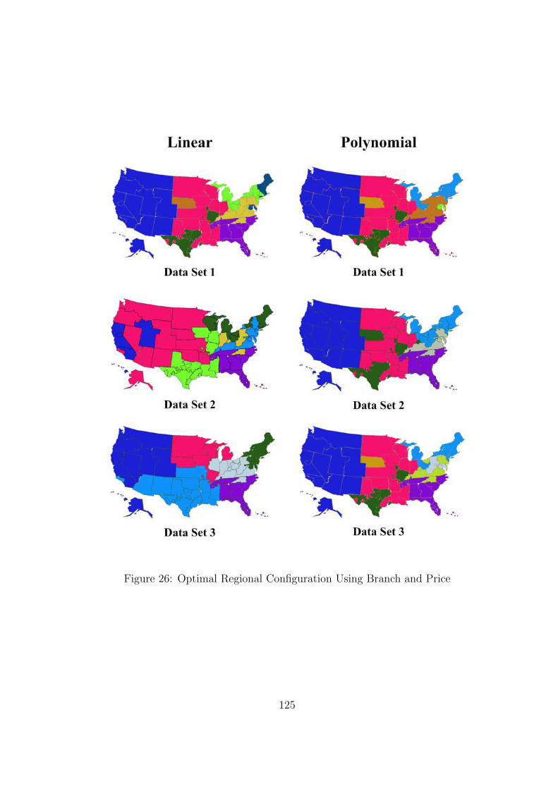
Figure 26: Optimal Regional Configuration Using Branch and Price
125

Figure 27: Optimal Regional Configuration Using Branch and Price (Contd.)
Table 18: Improvement on Intra-regional Transplant Cardinality (using Branch and Price)
Data Set 1 2 3 4
Simulation 37.3 39.5 52.3 31.9
Linear Analytic 96.1 104.5 108.4 113.5
Simulation 42.7 50.2 55.5 44.6
Polynomial Analytic 93.3 103.7 101.1 101.6
126

Table 19: Paired t Test: Branch and Price vs. Explicit Region Enumeration (Linear)
Paired Differences
Data Std. Std. Error 95% CI of the Diff.
Set Mean Deviation Mean Lower Upper t Sig.
1 36.95 53.29 9.73 17.05 56.84 3.797 .001
2 50.08 49.64 9.06 31.55 68.62 5.526 .000
3 90.48 48.53 8.86 72.36 108.6 10.21 .000
4 2.71 47.57 8.68 -15.05 20.48 0.313 .757
Table 20: Paired t Test: Branch and Price vs. Explicit Region Enumeration (Polynomial)
Paired Differences
Data Std. Std. Error 95% CI of the Diff.
Set Mean Deviation Mean Lower Upper t Sig.
1 47.27 53.11 9.70 27.44 67.10 4.875 .000
2 76.56 54.46 9.94 56.23 96.90 7.700 .000
3 82.21 47.26 8.63 64.56 99.85 9.527 .000
4 94.89 37.63 6.87 80.83 108.9 13.81 .000
127

of two constants, 0.9 or 1.1. Therefore, one instance corresponds to 0.9 and the other one
corresponds to 1.1. Recall that these notations are introduced in Chapters 3 and 4. In gen-
eral, these instances are easier than the real instance. The following tables of computational
results show this. An intuitive explanation is that national allocation has relatively little
effect, i.e.,l0ilij
is relatively small for all i, j ∈ I, and thus the pricing problem tends to be
easy.
Geographic Decomposition
We test the effect of geographic decomposition by designing various collections of region
covers. We solve the region design problem with the above coefficient specification based
on those region covers designs. For each design, we solve the region design problem by
applying column generation in which each pricing problem is constructed based on one
cover of the design and all integer feasible columns encountered in the pricing problem
solution process are added to the restricted master problem. Consequently, we obtain an
optimal regional configuration associated with the design. As a mnemonic, the region covers
designs are named m-n-k, where m is the number of region covers, n is the number of
OPOs in each region cover, and k is the region covers design index. Table 21 reports the
characteristics of region covers designs. In the table, we present three metrics in columns
“Total # Duplicates”, “Average # Duplicates”, and “# Appearance Max & Min”. Their
explanations are as follows. The total number of duplicates is m×n that measures how much
overlapping the covers are in a design. The average number of duplicates is the division of
the total number of duplicates by the number of OPOs. It measures how frequently an OPO
appears in a design. The maximum and minimum numbers of appearance are the maximum
and minimum numbers of times that an OPO appears in a design. These three metrics help
assess the design a priori. It is worth noting that in some designs, we intentionally exclude
one OPO. Table 21 also reports the objective value associated with each terminating regional
configuration and the best CPU time taken to obtain each terminating configuration. From
the table, we can see that the objective value tends to be larger as m or n increases. Between
two designs with the same m and n, a better solution is likely to be provided by a design
with larger maximum and minimum numbers of OPO appearance. On the other hand, as m
and n increase, the solution time increases. This is because more pricing problems need to
128
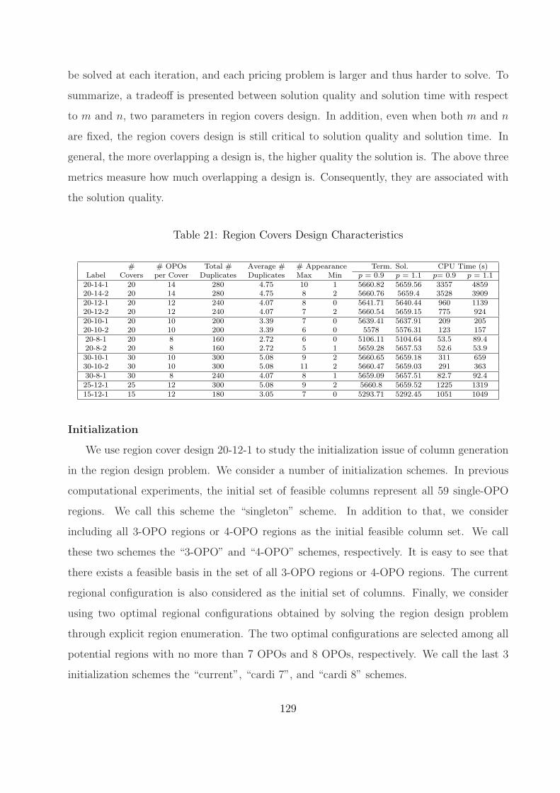
be solved at each iteration, and each pricing problem is larger and thus harder to solve. To
summarize, a tradeoff is presented between solution quality and solution time with respect
to m and n, two parameters in region covers design. In addition, even when both m and n
are fixed, the region covers design is still critical to solution quality and solution time. In
general, the more overlapping a design is, the higher quality the solution is. The above three
metrics measure how much overlapping a design is. Consequently, they are associated with
the solution quality.
Table 21: Region Covers Design Characteristics
# # OPOs Total # Average # # Appearance Term. Sol. CPU Time (s)Label Covers per Cover Duplicates Duplicates Max Min p = 0.9 p = 1.1 p= 0.9 p = 1.1
20-14-1 20 14 280 4.75 10 1 5660.82 5659.56 3357 485920-14-2 20 14 280 4.75 8 2 5660.76 5659.4 3528 390920-12-1 20 12 240 4.07 8 0 5641.71 5640.44 960 113920-12-2 20 12 240 4.07 7 2 5660.54 5659.15 775 92420-10-1 20 10 200 3.39 7 0 5639.41 5637.91 209 20520-10-2 20 10 200 3.39 6 0 5578 5576.31 123 15720-8-1 20 8 160 2.72 6 0 5106.11 5104.64 53.5 89.420-8-2 20 8 160 2.72 5 1 5659.28 5657.53 52.6 53.930-10-1 30 10 300 5.08 9 2 5660.65 5659.18 311 65930-10-2 30 10 300 5.08 11 2 5660.47 5659.03 291 36330-8-1 30 8 240 4.07 8 1 5659.09 5657.51 82.7 92.425-12-1 25 12 300 5.08 9 2 5660.8 5659.52 1225 131915-12-1 15 12 180 3.05 7 0 5293.71 5292.45 1051 1049
Initialization
We use region cover design 20-12-1 to study the initialization issue of column generation
in the region design problem. We consider a number of initialization schemes. In previous
computational experiments, the initial set of feasible columns represent all 59 single-OPO
regions. We call this scheme the “singleton” scheme. In addition to that, we consider
including all 3-OPO regions or 4-OPO regions as the initial feasible column set. We call
these two schemes the “3-OPO” and “4-OPO” schemes, respectively. It is easy to see that
there exists a feasible basis in the set of all 3-OPO regions or 4-OPO regions. The current
regional configuration is also considered as the initial set of columns. Finally, we consider
using two optimal regional configurations obtained by solving the region design problem
through explicit region enumeration. The two optimal configurations are selected among all
potential regions with no more than 7 OPOs and 8 OPOs, respectively. We call the last 3
initialization schemes the “current”, “cardi 7”, and “cardi 8” schemes.
129
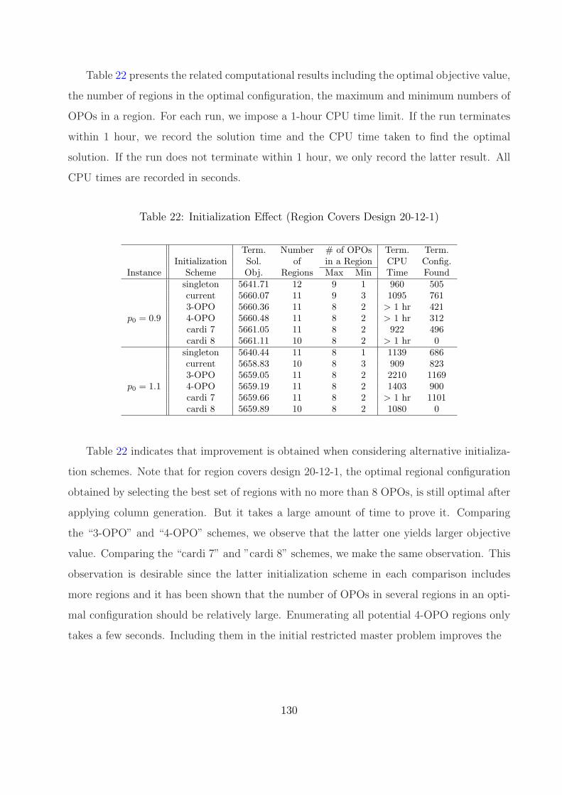
Table 22 presents the related computational results including the optimal objective value,
the number of regions in the optimal configuration, the maximum and minimum numbers of
OPOs in a region. For each run, we impose a 1-hour CPU time limit. If the run terminates
within 1 hour, we record the solution time and the CPU time taken to find the optimal
solution. If the run does not terminate within 1 hour, we only record the latter result. All
CPU times are recorded in seconds.
Table 22: Initialization Effect (Region Covers Design 20-12-1)
Term. Number # of OPOs Term. Term.Initialization Sol. of in a Region CPU Config.
Instance Scheme Obj. Regions Max Min Time Foundsingleton 5641.71 12 9 1 960 505current 5660.07 11 9 3 1095 7613-OPO 5660.36 11 8 2 > 1 hr 421
p0 = 0.9 4-OPO 5660.48 11 8 2 > 1 hr 312cardi 7 5661.05 11 8 2 922 496cardi 8 5661.11 10 8 2 > 1 hr 0
singleton 5640.44 11 8 1 1139 686current 5658.83 10 8 3 909 8233-OPO 5659.05 11 8 2 2210 1169
p0 = 1.1 4-OPO 5659.19 11 8 2 1403 900cardi 7 5659.66 11 8 2 > 1 hr 1101cardi 8 5659.89 10 8 2 1080 0
Table 22 indicates that improvement is obtained when considering alternative initializa-
tion schemes. Note that for region covers design 20-12-1, the optimal regional configuration
obtained by selecting the best set of regions with no more than 8 OPOs, is still optimal after
applying column generation. But it takes a large amount of time to prove it. Comparing
the “3-OPO” and “4-OPO” schemes, we observe that the latter one yields larger objective
value. Comparing the “cardi 7” and ”cardi 8” schemes, we make the same observation. This
observation is desirable since the latter initialization scheme in each comparison includes
more regions and it has been shown that the number of OPOs in several regions in an opti-
mal configuration should be relatively large. Enumerating all potential 4-OPO regions only
takes a few seconds. Including them in the initial restricted master problem improves the
130

solution significantly. One experiment left for future work is to see if enumerating all potential
regions with more OPOs would be benefit both in terms of the solution time and solution
quality since enumerating all 5-OPO regions or 6-OPO regions is still not too time-consuming.
Column Generation Strategy
For each region covers design, we consider a number of column generation strategies.
Strategy i, i = 1, . . . , 6, add at most first n feasible solutions per iteration to the iterative
restricted master problem (If there are fewer than n feasible solutions at any iteration, we
add all of them). Strategy “A” (“A” refers to all) adds all solutions per iteration (feasible
and optimal) to the iterative restricted master problem. Strategy “B” (“B” refers to best)
adds the optimal solution per iteration to the iterative restricted master problem. We present
related computational results for region covers designs 20-12-1 and 20-12-2 in Table 23. In
the column “CPU Time (s)” corresponding to each instance, we underscore the best CPU
time among the column generation strategies. In the next 2 columns corresponding to each
instance, we report the number of restricted master problems solved at the root node of the
search tree and the number of columns needed to solve the LP relaxation at the root node.
We also calculate the average numbers of columns generated at each iteration and for each
region cover. It is worth noting that most of computational effort is spent at the root node
for almost all instances. Related computational results for other region covers designs are
included in Appendix D. Among the various column generation strategies, Strategies 1, 2,
and “B” are always inferior with respect to the solution time. Strategy 3 is the best in 4
cases in terms of the solution time and Strategies 4, 5, 6, and “A” are the best in 8, 5, 8,
and 4 cases, respectively, in terms of the solution time. For almost all cases, the solution
time is comparable across the latter 4 strategies.
Strategies “A” and 1 normally take the fewest and most iterations, respectively. Strategy
“B” generates the fewest columns in most of the instances. However, Strategy 1 usually
generates the fewest columns on average per iteration. With Strategies 1 and 2, the average
number of columns added at each iteration is approximately proportional to the number of
columns allowed to generate per iteration. For instance, in case 20-12-1 with p0 = 1.1, the
average number of columns per iteration is 13.3 with Strategy 1, and the average number is
28.6 with Strategy 2. This indicates that allowing 3 or more columns per iteration would more
131
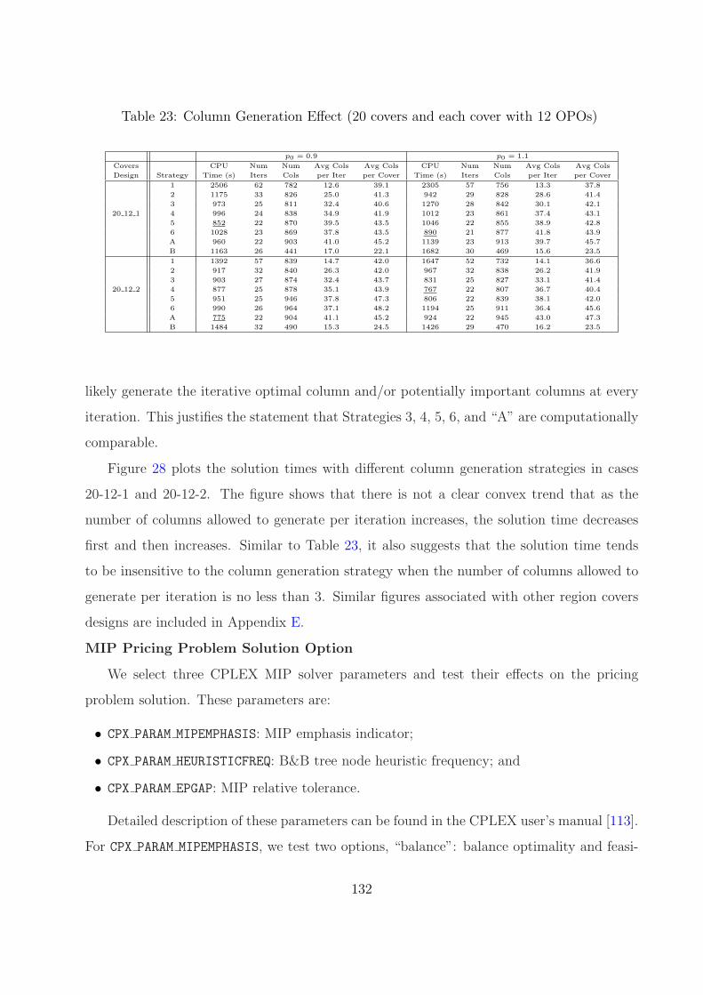
Table 23: Column Generation Effect (20 covers and each cover with 12 OPOs)
p0 = 0.9 p0 = 1.1
Covers CPU Num Num Avg Cols Avg Cols CPU Num Num Avg Cols Avg Cols
Design Strategy Time (s) Iters Cols per Iter per Cover Time (s) Iters Cols per Iter per Cover
1 2506 62 782 12.6 39.1 2305 57 756 13.3 37.8
2 1175 33 826 25.0 41.3 942 29 828 28.6 41.4
3 973 25 811 32.4 40.6 1270 28 842 30.1 42.1
20 12 1 4 996 24 838 34.9 41.9 1012 23 861 37.4 43.1
5 852 22 870 39.5 43.5 1046 22 855 38.9 42.8
6 1028 23 869 37.8 43.5 890 21 877 41.8 43.9
A 960 22 903 41.0 45.2 1139 23 913 39.7 45.7
B 1163 26 441 17.0 22.1 1682 30 469 15.6 23.5
1 1392 57 839 14.7 42.0 1647 52 732 14.1 36.6
2 917 32 840 26.3 42.0 967 32 838 26.2 41.9
3 903 27 874 32.4 43.7 831 25 827 33.1 41.4
20 12 2 4 877 25 878 35.1 43.9 767 22 807 36.7 40.4
5 951 25 946 37.8 47.3 806 22 839 38.1 42.0
6 990 26 964 37.1 48.2 1194 25 911 36.4 45.6
A 775 22 904 41.1 45.2 924 22 945 43.0 47.3
B 1484 32 490 15.3 24.5 1426 29 470 16.2 23.5
likely generate the iterative optimal column and/or potentially important columns at every
iteration. This justifies the statement that Strategies 3, 4, 5, 6, and “A” are computationally
comparable.
Figure 28 plots the solution times with different column generation strategies in cases
20-12-1 and 20-12-2. The figure shows that there is not a clear convex trend that as the
number of columns allowed to generate per iteration increases, the solution time decreases
first and then increases. Similar to Table 23, it also suggests that the solution time tends
to be insensitive to the column generation strategy when the number of columns allowed to
generate per iteration is no less than 3. Similar figures associated with other region covers
designs are included in Appendix E.
MIP Pricing Problem Solution Option
We select three CPLEX MIP solver parameters and test their effects on the pricing
problem solution. These parameters are:
• CPX PARAM MIPEMPHASIS: MIP emphasis indicator;
• CPX PARAM HEURISTICFREQ: B&B tree node heuristic frequency; and
• CPX PARAM EPGAP: MIP relative tolerance.
Detailed description of these parameters can be found in the CPLEX user’s manual [113].
For CPX PARAM MIPEMPHASIS, we test two options, “balance”: balance optimality and feasi-
132

Figure 28: Column Generation Effect (20 covers and each cover with 12 OPOs)
bility; and “feasibility”: emphasis on feasibility over optimality. For CPX PARAM HEURFREQ,
we test four options: “none”: not use the node heuristic; “automatic”: use it automatically
1: use it every iteration, “10”: use it every 10 iterations. We also choose the MIP relative
tolerance as 10−4, 5%, and 10%. Therefore, for each instance and a specified region covers
design, there are totally 24 pricing problem solution options. We run these experiments with
Strategy “A”, adding all solutions (feasible and optimal) to the restricted master problem
at each iteration. In Tables 24, we report the solution time, the number of restricted master
problems solved at the root node of the search tree, and the number of columns needed to
solve the LP relaxation at the root node. We underline the best solution time among the
24 options for each instance given a region covers design. Related computational results for
other region covers designs are included in Appendix F.
Among the 4 CPX PARAM HEURFREQ options, the option “none” is always the dominant
one. This strongly argues that applying the node heuristic is not effective. The computa-
tional results also show that for other two parameters, there is no evidence that one option
133

Table 24: Pricing Problem Solution Options: Design (20,12)
Solution Options p0 = 0.9 p0 = 1.1
MIP Heuristic MIP # # # #
Instance Emphasis Frequency Gap CPU (s) Iters Cols CPU (s) Iters Cols
feasibility none 10−4 781 20 944 1044 21 993
feasibility none 5% 803 20 904 1142 21 937
feasibility none 10% 764 19 908 899 19 928
feasibility automatic 10−4 1172 23 952 913 19 892
feasibility automatic 5% 816 20 790 1389 22 898
feasibility automatic 10% 839 19 797 1180 22 954
feasibility 1 10−4 2421 21 882 3355 22 947
feasibility 1 5% 2714 22 849 3595 24 835
feasibility 1 10% 3162 23 848 3579 22 912
feasibility 10 10−4 997 21 947 1413 22 952
feasibility 10 5% 1162 22 808 1266 22 874
20 12 1 feasibility 10 10% 1019 20 830 1257 21 945
balance none 10−4 833 22 729 914 23 754
balance none 5% 872 23 738 867 22 774
balance none 10% 957 24 760 971 23 759
balance none 10−4 973 22 903 1130 23 913
balance automatic 5% 985 22 820 1177 24 889
balance automatic 10% 1033 23 835 1434 25 855
balance 1 10−4 1907 21 903 2588 22 892
balance 1 5% 1968 21 875 2454 22 860
balance 1 10% 2236 21 795 2593 23 913
balance 10 10−4 911 22 822 1140 22 895
balance 10 5% 823 20 834 1058 21 830
balance 10 10% 1052 22 904 959 20 743
feasibility none 10−4 691 20 1045 710 19 873
feasibility none 5% 655 19 943 814 19 957
feasibility none 10% 783 21 972 1039 24 966
feasibility automatic 10−4 807 21 945 929 22 987
feasibility automatic 5% 804 22 802 926 22 958
feasibility automatic 10% 898 22 834 962 22 896
feasibility 1 10−4 2100 21 947 2176 20 944
feasibility 1 5% 2482 22 916 3080 24 976
feasibility 1 10% 1966 21 902 2986 23 857
feasibility 10 10−4 850 21 961 817 19 883
feasibility 10 5% 913 22 894 1029 21 908
20 12 2 feasibility 10 10% 1027 23 958 783 23 781
balance none 10−4 562 21 737 739 22 738
balance none 5% 562 21 737 739 22 738
balance none 10% 648 22 726 703 22 740
balance automatic 10−4 776 22 904 926 22 945
balance automatic 5% 786 22 874 924 23 879
balance automatic 10% 877 23 874 1042 24 849
balance 1 10−4 1778 22 888 2003 22 953
balance 1 5% 1713 22 904 2277 23 881
balance 1 10% 2011 23 865 1994 22 883
balance 10 10−4 928 24 961 934 22 909
balance 10 5% 814 21 849 947 22 816
balance 10 10% 804 22 875 812 21 811
134
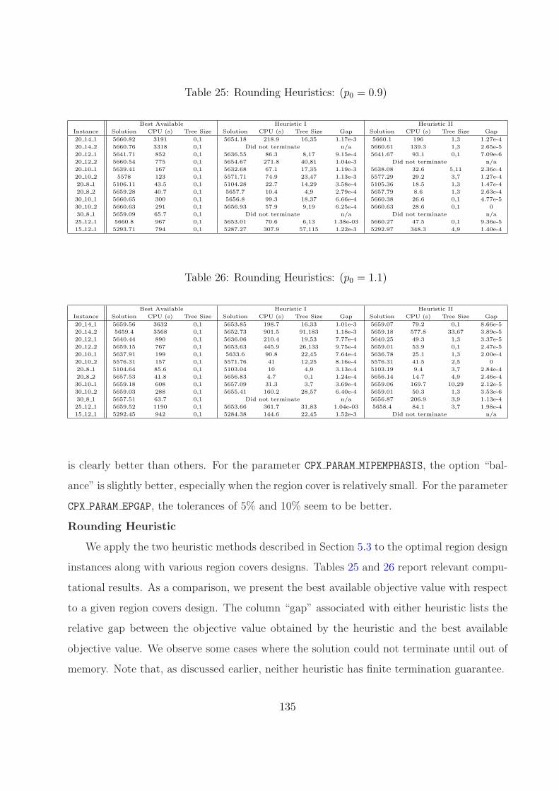
Table 25: Rounding Heuristics: (p0 = 0.9)
Best Available Heuristic I Heuristic II
Instance Solution CPU (s) Tree Size Solution CPU (s) Tree Size Gap Solution CPU (s) Tree Size Gap
20 14 1 5660.82 3191 0,1 5654.18 218.9 16,35 1.17e-3 5660.1 196 1,3 1.27e-4
20 14 2 5660.76 3318 0,1 Did not terminate n/a 5660.61 139.3 1,3 2.65e-5
20 12 1 5641.71 852 0,1 5636.55 86.3 8,17 9.15e-4 5641.67 93.1 0,1 7.09e-6
20 12 2 5660.54 775 0,1 5654.67 271.8 40,81 1.04e-3 Did not terminate n/a
20 10 1 5639.41 167 0,1 5632.68 67.1 17,35 1.19e-3 5638.08 32.6 5,11 2.36e-4
20 10 2 5578 123 0,1 5571.71 74.9 23,47 1.13e-3 5577.29 29.2 3,7 1.27e-4
20 8 1 5106.11 43.5 0,1 5104.28 22.7 14,29 3.58e-4 5105.36 18.5 1,3 1.47e-4
20 8 2 5659.28 40.7 0,1 5657.7 10.4 4,9 2.79e-4 5657.79 8.6 1,3 2.63e-4
30 10 1 5660.65 300 0,1 5656.8 99.3 18,37 6.66e-4 5660.38 26.6 0,1 4.77e-5
30 10 2 5660.63 291 0,1 5656.93 57.9 9,19 6.25e-4 5660.63 28.6 0,1 0
30 8 1 5659.09 65.7 0,1 Did not terminate n/a Did not terminate n/a
25 12 1 5660.8 967 0,1 5653.01 70.6 6,13 1.38e-03 5660.27 47.5 0,1 9.36e-5
15 12 1 5293.71 794 0,1 5287.27 307.9 57,115 1.22e-3 5292.97 348.3 4,9 1.40e-4
Table 26: Rounding Heuristics: (p0 = 1.1)
Best Available Heuristic I Heuristic II
Instance Solution CPU (s) Tree Size Solution CPU (s) Tree Size Gap Solution CPU (s) Tree Size Gap
20 14 1 5659.56 3632 0,1 5653.85 198.7 16,33 1.01e-3 5659.07 79.2 0,1 8.66e-5
20 14 2 5659.4 3568 0,1 5652.73 901.5 91,183 1.18e-3 5659.18 577.8 33,67 3.89e-5
20 12 1 5640.44 890 0,1 5636.06 210.4 19,53 7.77e-4 5640.25 49.3 1,3 3.37e-5
20 12 2 5659.15 767 0,1 5653.63 445.9 26,133 9.75e-4 5659.01 53.9 0,1 2.47e-5
20 10 1 5637.91 199 0,1 5633.6 90.8 22,45 7.64e-4 5636.78 25.1 1,3 2.00e-4
20 10 2 5576.31 157 0,1 5571.76 41 12,25 8.16e-4 5576.31 41.5 2,5 0
20 8 1 5104.64 85.6 0,1 5103.04 10 4,9 3.13e-4 5103.19 9.4 3,7 2.84e-4
20 8 2 5657.53 41.8 0,1 5656.83 4.7 0,1 1.24e-4 5656.14 14.7 4,9 2.46e-4
30 10 1 5659.18 608 0,1 5657.09 31.3 3,7 3.69e-4 5659.06 169.7 10,29 2.12e-5
30 10 2 5659.03 288 0,1 5655.41 160.2 28,57 6.40e-4 5659.01 50.3 1,3 3.53e-6
30 8 1 5657.51 63.7 0,1 Did not terminate n/a 5656.87 206.9 3,9 1.13e-4
25 12 1 5659.52 1190 0,1 5653.66 361.7 31,83 1.04e-03 5658.4 84.1 3,7 1.98e-4
15 12 1 5292.45 942 0,1 5284.38 144.6 22,45 1.52e-3 Did not terminate n/a
is clearly better than others. For the parameter CPX PARAM MIPEMPHASIS, the option “bal-
ance” is slightly better, especially when the region cover is relatively small. For the parameter
CPX PARAM EPGAP, the tolerances of 5% and 10% seem to be better.
Rounding Heuristic
We apply the two heuristic methods described in Section 5.3 to the optimal region design
instances along with various region covers designs. Tables 25 and 26 report relevant compu-
tational results. As a comparison, we present the best available objective value with respect
to a given region covers design. The column “gap” associated with either heuristic lists the
relative gap between the objective value obtained by the heuristic and the best available
objective value. We observe some cases where the solution could not terminate until out of
memory. Note that, as discussed earlier, neither heuristic has finite termination guarantee.
135

Tables 25 and 26 show that both heuristics are fast. It is also intuitive that the second
heuristic is faster than the first one in most of the instances since with the second heuristic,
the columns generated per iteration should be much more likely “promising”. The tables
also show that both heuristics yield high-quality suboptimal solutions. In all instances,
the second heuristic provides a larger suboptimal solution. Another observation is that the
branch-and-price tree size could be large when applying these heuristics.
136

6.0 IMPROVING THE SOLUTION OF THE PRICING PROBLEM
From the analysis in Chapter 5, we know that our mixed-integer pricing problem does not
possess the integrality property. It is both theoretically and practically hard to solve. Hence,
the most computationally intensive component of the branch-and-price algorithm is the
solution of the pricing problem. In Chapter 5, we make several attempts to mitigate this
major bottleneck in the branch-and-price algorithm. For example, we apply geographic
decomposition to solve smaller-scale pricing problems. However, all these attempts do not
fundamentally improve the pricing problem solution. In this chapter, we will discuss how
to make the solution of the pricing problem more efficient using the following two ideas.
The first idea is to study various formulations of the pricing problem and ultimately find
an alternative that achieves more efficient solution. The second one is to study the pricing
problem polyhedron and add strong valid inequalities for the pricing problem to achieve
more efficient solution.
In Section 6.1, we present three alternative formulations in addition to the one presented
in Chapter 5. We analyze and compare these alternatives. These alternative formulations
are obtained by either replacing or combining existing decision variables. It turns out that
together with the original formulation, they are theoretically equivalent, meaning that among
the four formulations, the optimal objective value is identical and there exists an identical
optimal set of OPOs. However, computationally the four formulations perform differently.
In Section 6.2, we develop two classes of valid inequalities. Our objective is to improve the
solution of the pricing problem with incorporation of these valid inequalities. We present
related theoretical results and explore the possibility of embedding them in a branch-and-
bound solution. We report our computational findings in Section 6.3. In this chapter, we
137
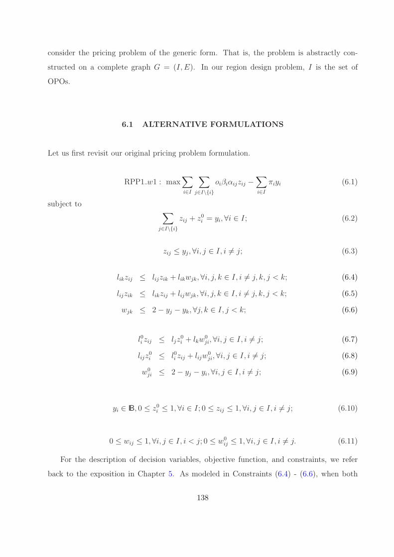
consider the pricing problem of the generic form. That is, the problem is abstractly con-
structed on a complete graph G = (I, E). In our region design problem, I is the set of
OPOs.
6.1 ALTERNATIVE FORMULATIONS
Let us first revisit our original pricing problem formulation.
RPP1 w1 : max∑
i∈I
∑
j∈I\{i}oiβiαijzij −
∑
i∈I
πiyi (6.1)
subject to∑
j∈I\{i}zij + z0
i = yi,∀i ∈ I; (6.2)
zij ≤ yj,∀i, j ∈ I, i 6= j; (6.3)
likzij ≤ lijzik + likwjk,∀i, j, k ∈ I, i 6= j, k, j < k; (6.4)
lijzik ≤ likzij + lijwjk,∀i, j, k ∈ I, i 6= j, k, j < k; (6.5)
wjk ≤ 2− yj − yk,∀j, k ∈ I, j < k; (6.6)
l0i zij ≤ ljz0i + lkw
0ji,∀i, j ∈ I, i 6= j; (6.7)
lijz0i ≤ l0i zij + lijw
0ji,∀i, j ∈ I, i 6= j; (6.8)
w0ji ≤ 2− yj − yi,∀i, j ∈ I, i 6= j; (6.9)
yi ∈ IB, 0 ≤ z0i ≤ 1,∀i ∈ I; 0 ≤ zij ≤ 1,∀i, j ∈ I, i 6= j; (6.10)
0 ≤ wij ≤ 1,∀i, j ∈ I, i < j; 0 ≤ w0ij ≤ 1,∀i, j ∈ I, i 6= j. (6.11)
For the description of decision variables, objective function, and constraints, we refer
back to the exposition in Chapter 5. As modeled in Constraints (6.4) - (6.6), when both
138

nodes j and k are selected, i.e., yj = yk = 1, wjk = 0, and thus a proportionality constraint
is imposed for flow from node i to nodes j and k. On the other hand, at most one node being
selected between j and k implies that there is no additional restriction on wjk other than its
upper bound. A similar argument applies to w0jk and w0
kj. To summarize, when yj = yk = 1,
wjk = w0jk = w0
kj = 0; when yjyk = 0, 0 ≤ wjk, w0jk, w
0kj ≤ 1.
Proposition 6.1. Assume that oj, βj, αjk ≥ 0 for all j, k ∈ I. If yj = 0 or yk = 0 for any j
and k, there exists some optimal solution to RPP w1 such that wjk = w0jk = w0
kj = 1.
Proof. Let us prove this result by contradiction. Suppose that in any optimal solution to
RPP w1, there exists a node j ∈ I such that yj = 0, wjk < 1 or w0jk < 1 or w0
kj < 1 for some
node k ∈ I, k 6= j. Without loss of generality, let us assume that in an optimal solution
(y, z, z0, w, w0), there exists a node j such that yj = 0, we have wjk < 1 for some node k.
Therefore, Constraint (6.6) is not tight regardless of the value of yk. In addition, we know
zij = 0 for any i ∈ I. Let us arbitrarily pick an i, zij = 0 implies that Constraint (6.4)
is not tight and Constraint (6.5) becomes zik ≤ wjk. Let w′jk = wjk + ǫ = 1. It is easy
to verify that both Constraints (6.4) and (6.5) are satisfied by the solution (y, z, z0, w′, w0)
where we replace wjk with w′jk. The condition that oi, βi, αij, αik ≥ 0 for all i ∈ I implies
that (y, z, z0, w′, w0) is also an optimal solution. Hence, a contradiction occurs and the result
follows.
Proposition 6.1 provides a way to modify the pricing problem formulation. From the
proposition, we know there exists some optimal solution to RPP w1 such that wjk = w0jk =
w0kj = 1 if yj yk = 0 or yj + yk ≤ 1. Note that the above proof also indirectly indicates that
increasing the value of wjk does not affect yj or yk. Since our pricing problem solution is
139

to provide an optimal set of nodes (forming a column that prices out favorably) to the
restricted master problem, we can replace wjk, w0jk, and w0
kj with one variable wjk. The
modified formulation is presented as:
RPP w2 : max∑
i∈I
∑
j∈I\{i}oiβiαijzij −
∑
i∈I
πiyi (6.12)
subject to
(6.2), (6.3), (6.10);
likzij ≤ lijzik + likwjk,∀i, j, k ∈ I, i 6= j, k, j < k; (6.13)
lijzik ≤ likzij + lijwjk,∀i, j, k ∈ I, i 6= j, k, j < k; (6.14)
l0i zij ≤ lijz0i + l0i wij,∀i, j ∈ I, i < j; (6.15)
lijz0i ≤ l0i zij + lijwij,∀i, j ∈ I, i < j; (6.16)
l0jzji ≤ ljiz0j + l0jwij,∀i, j ∈ I, i < j; (6.17)
ljiz0j ≤ l0jzji + ljiwij,∀i, j ∈ I, i < j; (6.18)
wij ≤ 2− yi − yj,∀i, j ∈ I, i < j; (6.19)
0 ≤ wij ≤ 1,∀i, j ∈ I, i < j. (6.20)
Note that RPP w2 does not change flow constraints (6.2) and (6.3), and bounding con-
straint (6.10). We therefore use their equation numbers in RPP w2 as well as other alter-
native formulations presented later in this section. Let ujk = 1 − wjk and u0jk = 1 − w0
jk.
Then when yj = yk = 1, ujk = u0jk = u0
kj = 1 and when yjyk = 0, ujk = u0jk = u0
kj = 0. We
consider the following alternative formulation where we substitute wjk with 1− ujk and w0jk
with 1− u0jk in RPP w1.
RPP u1 : max∑
i∈I
∑
j∈I\{i}oiβiαijzij −
∑
i∈I
πiyi (6.21)
subject to
(6.2), (6.3), (6.10);
140

likzij + likujk ≤ lijzik + lik,∀i, j, k ∈ I, i 6= j, k, j < k; (6.22)
lijzik + lijujk ≤ likzij + lij,∀i, j, k ∈ I, i 6= j, k, j < k; (6.23)
ujk ≥ yj + yk − 1,∀i, j ∈ I, i < j; (6.24)
ujk ≤ yj,∀i, j ∈ I, i < j; (6.25)
ujk ≤ yk,∀i, j ∈ I, i < j; (6.26)
l0i zij + l0i u0ji ≤ lijz
0i + l0i ,∀i, j ∈ I, i 6= j; (6.27)
lijz0i + liju
0ji ≤ l0i zij + lij,∀i, j ∈ I, i 6= j; (6.28)
u0ji ≥ yi + yj − 1,∀i, j ∈ I, j 6= i; (6.29)
u0ji ≤ yi,∀i, j ∈ I, j 6= i; (6.30)
u0ji ≤ yj,∀i, j ∈ I, j 6= i; (6.31)
0 ≤ uij ≤ 1,∀i, j ∈ I, i < j; 0 ≤ u0ji ≤ 1,∀i, j ∈ I, j 6= i. (6.32)
Given the relationship between wjk and ujk, Constraints (6.22) - (6.24) and (6.27) - (6.29)
in RPP u1 correspond to Constraints (6.4) - (6.6) and (6.7) - (6.9), respectively.
Corollary 6.1. Assume that oj, βj, αjk ≥ 0 for all j, k ∈ I. If yj = 0 or yk = 0 for any
j, k ∈ I, there exists some optimal solution to RPP u1 such that ujk = u0jk = u0
kj = 0.
Proof. The results follows directly from Proposition 6.1.
Proposition 6.2. Assume that oj, βj, αjk ≥ 0 for all j, k ∈ I. Let v be the optimal objective
value of RPP u1 and v′ be the optimal objective value of RPP u1 without Constraints (6.25)
- (6.26) and (6.30) - (6.31). Then v = v′.
Proof. It is clear that v ≤ v′. Now let us prove that v ≥ v′. Let (y, z, z0, u, u0) be an optimal
solution to RPP u1 excluding Constraints (6.25) - (6.26) and (6.30) - (6.31). If yj = yk = 1
for any pair j, k ∈ I, ujk = 1, which can be obtained by Constraint (6.24) and the associated
bounding constraint. A similar argument applies to u0ji. In this case, Constraints (6.25)
- (6.26) and (6.30) - (6.31) are identical to the upper bounds on the variables. Hence,
141
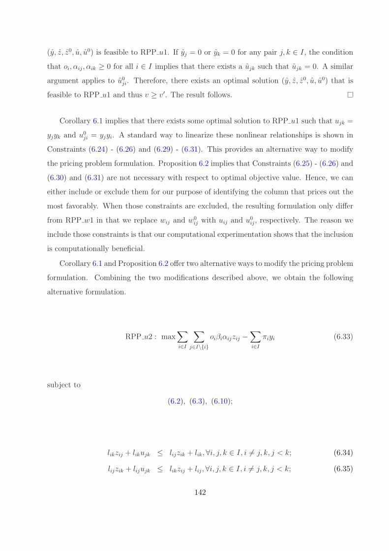
(y, z, z0, u, u0) is feasible to RPP u1. If yj = 0 or yk = 0 for any pair j, k ∈ I, the condition
that oi, αij, αik ≥ 0 for all i ∈ I implies that there exists a ujk such that ujk = 0. A similar
argument applies to u0ji. Therefore, there exists an optimal solution (y, z, z0, u, u0) that is
feasible to RPP u1 and thus v ≥ v′. The result follows.
Corollary 6.1 implies that there exists some optimal solution to RPP u1 such that ujk =
yjyk and u0ji = yjyi. A standard way to linearize these nonlinear relationships is shown in
Constraints (6.24) - (6.26) and (6.29) - (6.31). This provides an alternative way to modify
the pricing problem formulation. Proposition 6.2 implies that Constraints (6.25) - (6.26) and
(6.30) and (6.31) are not necessary with respect to optimal objective value. Hence, we can
either include or exclude them for our purpose of identifying the column that prices out the
most favorably. When those constraints are excluded, the resulting formulation only differ
from RPP w1 in that we replace wij and w0ij with uij and u0
ij, respectively. The reason we
include those constraints is that our computational experimentation shows that the inclusion
is computationally beneficial.
Corollary 6.1 and Proposition 6.2 offer two alternative ways to modify the pricing problem
formulation. Combining the two modifications described above, we obtain the following
alternative formulation.
RPP u2 : max∑
i∈I
∑
j∈I\{i}oiβiαijzij −
∑
i∈I
πiyi (6.33)
subject to
(6.2), (6.3), (6.10);
likzij + likujk ≤ lijzik + lik,∀i, j, k ∈ I, i 6= j, k, j < k; (6.34)
lijzik + lijujk ≤ likzij + lij,∀i, j, k ∈ I, i 6= j, k, j < k; (6.35)
142

l0i zij + l0i uij ≤ lijz0i + l0i ,∀i, j ∈ I, i < j; (6.36)
lijz0i + lijuij ≤ l0i zij + lij,∀i, j ∈ I, i < j; (6.37)
l0jzji + l0juij ≤ ljiz0j + l0j ,∀i, j ∈ I, i < j; (6.38)
ljiz0j + ljiuij ≤ l0jzji + lji,∀i, j ∈ I, i < j; (6.39)
uij ≥ yi + yj − 1,∀i, j ∈ I, i < j; (6.40)
uij ≤ yi,∀i, j ∈ I, i < j; (6.41)
uij ≤ yj,∀i, j ∈ I, i < j; (6.42)
0 ≤ uij ≤ 1,∀i, j ∈ I, i < j. (6.43)
With Propositions 6.1 and 6.2, and Corollary 6.1, we are ready to show the equivalence
of the above four alternative formulations in terms of the optimal objective value.
Theorem 6.1. Let z∗w1, z∗w2, z∗u1, and z∗u2 be the optimal objective values of RPP w1,
RPP w2, RPP u1, and RPP u2, respectively. Then we have
z∗w1 = z∗w2 = z∗u1 = z∗u2.
Furthermore, there exists an optimal solution to each problem in which decision variables y
are identical among the four formulations.
Proof. The equivalence of RPP w1 and RPP w2 follows from Proposition 6.1. The equiva-
lence of RPP u1 and RPP u2 follows from Corollary 6.1. The equivalence of RPP w1 and
RPP u1 is established by Proposition 6.2 and the fact that it is a simple relation linking wij
with uij and w0ij with u0
ij for all i, j ∈ I. We can establish the equivalence between RPP w2
and RPP u2 in the same manner.
Corollary 6.2. Let zLPw1 , zLP
w2 , zLPu1 , zLP
u2 be the optimal objective values of the LP relaxation
of RPP w1, RPP w2, RPP u1, and RPP u2, respectively. Then we have
zLPw1 = zLP
w2 = zLPu1 = zLP
u2 .
143

Let us use RPP u2 to explain the above results intuitively. With the assumption that
oi, βi, αij ≥ 0 for all i, j ∈ I, there is no incentive to increase uij and u0ij in any above
formulation. Hence, there exists an optimal solution such that both Constraint (6.40) and
the lower bounding constraint on uij or u0ij are tight for all i, j ∈ I. It is clear that none of
our formulation modifications affects this fact.
To summarize, various alternative formulations are induced by using w variables or u
variables, setting wij = w0ij = w0
ji or uij = u0ij = u0
ji, and including Constraints (6.41) and
(6.42). These formulations yield the same optimal objective value in their respective LP
relaxations. However, the solution times and initial LP gaps of these LP relaxations may
differ a lot when using the CPLEX MIP solver. In Section 6.3.1 we will compare these
alternative formulations computationally. Our computational results indicate that solving
RPP u2 tends to take the least amount of time. Therefore, we conduct a polyhedral study
on RPP u2 in the next section.
6.2 POLYHEDRAL STUDY
In this section, we consider two classes of valid inequalities for RPP u2. For ease of expo-
sition, we drop the label u2 in RPP u2. Note that with all three constraints (6.40) - (6.42)
included in RPP u2, we have the complete linearization of uij = yiyj for all i, j ∈ I. This
means that each uij can be viewed as a binary variable.
6.2.1 Valid Inequality Class I
For this class of valid inequalities, we study three mixed-integer programs derived from the
pricing problem RPP. We restrict RPP by adding constraints associated with the cardinality
of the optimal node set, i.e.,∑
i∈I y∗i = s,
∑
i∈I y∗i ≥ s,
∑
i∈I y∗i ≤ s, where y∗ is the incidence
vector of the optimal node set and s is given. Hence, such restrictions provides three mixed-
integer programs. With a given cardinality value s, we call the three resulting problems
RPP=(s), RPP≥(s), and RPP≤(s). A formal definition will be given later in this section.
144

We add valid inequalities for the resulting mixed-integer programs to make their solutions
more efficient. The main idea here is to solve many resulting mixed-integer programs instead
of dealing with RPP directly or its subproblems in a branch-and-bound solution. In this
way, we have to search for an cardinality which is the optimal cardinality of the node set.
In general, only a naıve approach is applicable that solves many of RPP=(s), RPP≥(s), and
RPP≤(s) for various s, which would not be desirable. However, often times we have some
idea on how many nodes are likely included in the optimal node set. Furthermore, some
efficient algorithmic procedures often exist in practice to search for the optimal cardinality
in our region design pricing problems. In this section, we will first present relevant theoretical
results for deriving the valid inequalities. Then we will discuss the special case and describe
three algorithmic procedures. At the end of this section, we consider how to incorporate
these valid inequalities in the branch-and-bound solution for RPP. For each i ∈ I, let us
rank {lij}, ∀j ∈ I, j 6= i, in ascending and descending orders, and denote {laij} and {ldij}
to be the sequences in ascending and descending orders, respectively. Define Lai (s,D) and
Ldi (s,D) to be the indices of the first s elements of D ⊆ I in the respective sequences. This
implies that 0 ≤ s ≤ |I| − 2. We assume that for any D ⊂ I, Lai (s,D) = Ld
i (s,D) = ∅ if
s = 0.
Proposition 6.3. Denote S ⊆ I to be the node set corresponding to a selected region. Let
s = |S| − 2. If i, j ∈ S, then
lijlij +
∑
k∈Ldi (s,I\{i,j}) lik + l0i
≤ zij ≤lij
lij +∑
k∈Lai (s,I\{i,j}) lik + l0i
.
Proof. Let us assume that S = {i, j, k1, k2, . . . , ks}. Then zij =lij
P
k∈S\{i,j} lik+lij+l0i. By def-
inition, we have∑
k∈Lai (s,I\{i,j}) lij ≤
∑
k∈S\{i,j} lik ≤∑
k∈Ldi (s,I\{i,j}) lij. Hence the result
follows.
Proposition 6.3 states that given a selected region, the intra-regional transplant likelihood
zij is bounded from above and below. The upper bound is obtained by selecting a number of
OPOs with the smallest transplant likelihoods from OPO i excluding lii and lij. The lower
bound is obtained by selecting a number of OPOs with the largest transplant likelihoods
from OPO i excluding lii and lij.
145

Proposition 6.4. Let RPP≥(s) be RPP with imposition of the following additional con-
straint:∑
i∈I yi ≥ s for s = 2, . . . , |I|. Then the following inequality is valid for RPP≥(s):
zij ≤lijuij
lij +∑
k∈Lai (s−2,I\{i,j}) lik + l0i
, (6.44)
for all i, j ∈ I, i 6= j.
Proof. It is easy to see the result in the case where uij = yiyj = 0. In the case where uij = 1,
i.e., yi = yj = 1, the result follows directly from Proposition 6.3 as s − 2 =∑
i∈I yi − 2 =
|S| − 2. If∑
i∈I yi = s′ > s, we have
zij ≤lij
lij +∑
k∈Lai (s′−2,I\{i,j}) lik + l0i
≤lij
lij +∑
k∈Lai (s−2,I\{i,j}) lik + l0i
.
The first inequality is due to Proposition 6.3. The second inequality holds for s′ > s and
uij = 1.
Proposition 6.5. Let RPP≤(s) be RPP with imposition of the following additional con-
straint:∑
i∈I yi ≤ s for s = 2, . . . , |I|. Then the following inequality is valid for RPP≤(s):
zij ≥lijuij
lij +∑
k∈Ldi (s−2,I\{i,j}) lik + l0i
, (6.45)
for all i, j ∈ I, i 6= j.
Proof. This proof is similar to the one in Proposition 6.4. It is easy to see the result in the
case where uij = yiyj = 0. In the case where uij = 1, i.e., yi = yj = 1, the result follows
directly from Proposition 6.3 as s− 2 =∑
i∈I yi − 2 = |S| − 2. If∑
i∈I yi = s′ < s, we have
zij ≥lij
lij +∑
k∈Ldi (s′−2,I\{i,j}) lik + l0i
≥lij
lij +∑
k∈Ldi (s−2,I\{i,j}) lik + l0i
.
The first inequality is due to Proposition 6.3. The second inequality holds for s′ < s and
uij = 1.
With respect to variable zij, we call Inequality (6.44) the upper bounding valid inequality
and call Inequality (6.45) the lower bounding valid inequality.
146

Corollary 6.3. The following inequality is valid for RPP:
lijuij∑
k∈I\{i} lik + l0i≤ zij ≤
lijuij
lij + l0i.
Proof. The upper bounding valid inequality follows from Propositions 6.4 as s = 2 and the
lower bounding valid inequality follows from Proposition 6.5 as s = |I|.
Theorem 6.2. Let RPP=(s) be RPP with imposition of the following additional constraint:∑
i∈I yi = s for s = 2, . . . , |I|. Then the following inequality is valid for RPP=(s):
lijuij
lij +∑
k∈Ldi (s−2,I\{i,j}) lik + l0i
≤ zij ≤lijuij
lij +∑
k∈Lai (s−2,I\{i,j}) lik + l0i
, and (6.46)
ljiuij
lji +∑
k∈Ldj (s−2,I\{i,j}) ljk + l0j
≤ zji ≤ljiuij
lji +∑
k∈Laj (s−2,I\{i,j}) ljk + l0j
, (6.47)
for all i, j ∈ I, i 6= j.
Proof. It is easy to see the result in the case where uij = 0. In the case where uij = 1, i.e.,
yi = yj = 1, the results follows directly from Proposition 6.3. The argument is the same as
in Propositions 6.4 and 6.5.
Remark 6.1. Let us denote P≥s and P≤
s to be the feasible solution regions of RPP≥(s) and
RPP≤(s), respectively. It is clear that P≥s+1 ⊆ P≥
s and P≤s ⊆ P≤
s+1, ∀s = 0, . . . , |I| − 1.
Remark 6.2. Any feasible solution to RPP=(s) is both a feasible solution to RPP≥(s) and
RPP≤(s).
Remark 6.3. Let us denote P=s to be the feasible solution region of RPP=(s). When s = |I|,
zij =pj
P
k∈I\{i} pk+p0i
, and P=s becomes one point (all z and u variables are uniquely deter-
mined). This corresponds to the case where all y variables are fixed to 1.
Results similar to those in Propositions 6.4 and 6.5 and Theorem 6.2 can also be applied
to impose valid bounding inequalities for variables z0i and yi. For example, Corollary 6.4 is
analogous to Theorem 6.2.
147

Corollary 6.4. For any s = 1, . . . , |I|, The following inequality is valid for RPP=(s):
l0i yi
l0i +∑
k∈Ldi (s−1,I\{i}) lik
≤ z0i ≤
l0i yi
l0i +∑
k∈Lai (s−1,I\{i}) lik
, (6.48)
for all i ∈ I.
Proof. It is easy to see the result in the case where yi = 0. Let us consider the case where
yi = 1. Denote S ⊆ I to be the node set corresponding to the selected region. Let s′ = |S|−1.
We assume that S = {i, k1, . . . , k′s}. Similar to Proposition 6.3, we have the following
statement. If i ∈ S, then
l0il0i +
∑
k∈Ldi (s′,I\{i}) lik
≤ z0i ≤
l0il0i +
∑
k∈Lai (s′,I\{i}) lik
. (6.49)
Let s = |S|. Since i ∈ S is equivalent to yi = 1, the result follows from (6.49).
Corollary 6.5. The following valid inequality is valid for RPP:
l0i yi∑
k∈I\{i} lik + l0i≤ z0
i ≤ yi.
Proof. Similar to the proof for Corollary 6.3, the result follows directly from Corollary 6.4.
Remark 6.4. Consider any OPO i, if we view the national level as an artificial OPO with
pure distribution likelihood l0i , Corollary 6.4 becomes a special case of Theorem 6.2 addressing
proportional allocation between this artificial OPO and other OPOs.
We explain the specification in Remark 6.4 as follows. Since uij = yiyj, we can replace
uij with yiyj. Whether zij is equal to 0 is dependent upon the value of uij, or in other words,
both yi and yj. Its physical interpretation in RPP is that allocation at the region level
from OPO i to j occurs only if both i and j are included in the selected region. Whether
z0i is equal to 0 is dependent upon the value of yi. Its physical interpretation in RPP is
that national-level allocation occurs at OPO i only if i is included in the selected region.
Note that an artificial OPO is associated with each OPO. Let y0i be the binary variable
representing the artificial OPO associated with OPO i. It is always true that y0i = yi and
thus yiy0i = yi.
148

So far, we have derived a class of valid inequalities. Unfortunately, most of them are
for the problems with additional set cardinality constraints:∑
i∈I yi ≥ s or∑
i∈I yi ≤ s. In
Corollaries 6.3 and 6.5, we present two inequalities that are valid for RPP. However, they are
not strong. Before solving the pricing problem, if we have some idea or restriction on how the
cardinality of the optimal set would be, we would impose stronger valid inequalities based
on Theorem 6.2 and Corollary 6.4. This procedure can be viewed as formulation tightening.
Johnson et al. [119] showed encouraging results when adding strong valid inequalities for
the pricing problem of the min-cut clustering problem [119] after a thorough investigation
of the pricing problem polytope.
In a special case regarding the pricing problem, we derive several algorithmic procedures
to search the optimal set cardinality by utilizing the relation among RPP≥(s) and RPP≤(s)
with various s. To compute RPP≥(s) and RPP≤(s), we add valid inequalities (6.46) - (6.47)
and (6.48) with respect to a specified s. In Section 6.2.1.1 we first present relevant general
theoretical results and then discuss several algorithmic procedures for a special case. More
generally, we use branch and bound to solve the orginal pricing problem. As the branch-
and-bound tree is developed, we can impose stronger valid inequalities at search tree nodes
besides the root node. Cut generation in a branch-and-bound solution framework is discussed
in Section 6.2.1.2.
6.2.1.1 Searching the Optimal Set Cardinality in a Special Case We define f≥(s)
and f≤(s) to be the optimal objective function values of RPP≥(s) and RPP≤(s), respectively.
We define f ∗ to be the optimal objective function value of RPP. Let us also define S∗ to
be the set that contains the number of nodes selected in an optimal solution to the pricing
problem (optimal cardinality set). For any s∗ ∈ S∗, we call s∗ optimal set cardinality. First
let us show monotonicity of f≥(·) and f≤(·) as functions.
149

Lemma 6.1. Let s∗ be an optimal set cardinality, i.e., s∗ ∈ S∗, f≥(s∗) = f≤(s∗) = f ∗.
Proof. For any s ∈ S∗, since RPP≥(s) has an additional constraint compared to RPP, we
have f≥(s) ≤ f ∗. We also know that f≥(s) ≥ f ∗ since∑
i∈I yi = s implies that the optimal
solution to RPP is a feasible solution to RPP≥(s). Similarly we can prove f≤(s) = f ∗ for
any s ∈ S∗.
Proposition 6.6. Let smin = min{s|s ∈ S∗} and smax = max{s|s ∈ S∗}. For s = 0, . . . , |I|,
• f≥(s) : ZZ+ 7→ IR is a monotonically nonincreasing function. Moreover, it is constant in
S≥ := {0, 1, . . . , smax}, i.e., f≥(s) = f ∗, ∀s ∈ S≥.
• f≤(s) : ZZ+ 7→ IR is a monotonically nondecreasing function. Moreover, it is constant in
S≤ := {smin, . . . , |I| − 1, |I|}, i.e., f≤(s) = f ∗, ∀s ∈ S≤.
Proof. We only prove the first part here. The second part can be proved in the same manner.
Following from the fact that P≥s+1 ⊆ P≥
s , we have f≥(s + 1) ≤ f≥(s), ∀s = 0, . . . , |I| − 1.
Suppose f≥(s) is not constant when s ∈ S≥. Due to its monotonicity, there must exist an
s′ ∈ S≥ such that f≥(s′) > f≥(s∗) for an s∗ ∈ S∗. However, for any s∗ ∈ S∗, f≥(s∗) = f ∗ ≥
f≥(s′) by Lemma 6.1. Thus the result is implied by the contradiction.
Proposition 6.6 shows that f≥(s) and f≤(s) are monotonically nonincreasing and non-
decreasing, respectively. A special case we consider here includes two assumptions:
(A6.1) The optimal cardinality set S∗ is an integrally continuous set, i.e., S∗ = [smin, smax]∩
ZZ+.
(A6.2) f≥(s) is monotonically decreasing over s = smax + 1, . . . , |I| and f≤(s) is monoton-
ically increasing over s = 0, . . . , smin − 1.
Define f=(s) to be the optimal objective value of RPP=(s). With the above further spec-
ification, the function f=(s) presents properties that are suitable for application of some
efficient algorithms that search the optimal set cardinality. Our computational experiments
suggest that the pricing problem in the region design problem is likely in this special case.
150
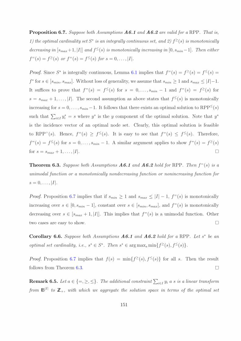
Proposition 6.7. Suppose both Assumptions A6.1 and A6.2 are valid for a RPP. That is,
1) the optimal cardinality set S∗ is an integrally continuous set, and 2) f≥(s) is monotonically
decreasing in [smax+1, |I|] and f≤(s) is monotonically increasing in [0, smin−1]. Then either
f=(s) = f≥(s) or f=(s) = f≤(s) for s = 0, . . . , |I|.
Proof. Since S∗ is integrally continuous, Lemma 6.1 implies that f=(s) = f≥(s) = f≤(s) =
f ∗ for s ∈ [smin, smax]. Without loss of generality, we assume that smin ≥ 1 and smax ≤ |I|−1.
It suffices to prove that f=(s) = f≤(s) for s = 0, . . . , smin − 1 and f=(s) = f≥(s) for
s = smax + 1, . . . , |I|. The second assumption as above states that f≤(s) is monotonically
increasing for s = 0, . . . , smin−1. It follows that there exists an optimal solution to RPP≤(s)
such that∑
i∈I y∗i = s where y∗ is the y component of the optimal solution. Note that y∗
is the incidence vector of an optimal node set. Clearly, this optimal solution is feasible
to RPP=(s). Hence, f=(s) ≥ f≤(s). It is easy to see that f=(s) ≤ f≤(s). Therefore,
f=(s) = f≤(s) for s = 0, . . . , smin − 1. A similar argument applies to show f=(s) = f≥(s)
for s = smax + 1, . . . , |I|.
Theorem 6.3. Suppose both Assumptions A6.1 and A6.2 hold for RPP. Then f=(s) is a
unimodal function or a monotonically nondecreasing function or nonincreasing function for
s = 0, . . . , |I|.
Proof. Proposition 6.7 implies that if smin ≥ 1 and smax ≤ |I| − 1, f=(s) is monotonically
increasing over s ∈ [0, smin − 1], constant over s ∈ [smin, smax], and f=(s) is monotonically
decreasing over s ∈ [smax + 1, |I|]. This implies that f=(s) is a unimodal function. Other
two cases are easy to show.
Corollary 6.6. Suppose both Assumptions A6.1 and A6.2 hold for a RPP. Let s∗ be an
optimal set cardinality, i.e., s∗ ∈ S∗. Then s∗ ∈ arg maxs min{f≥(s), f≤(s)}.
Proof. Proposition 6.7 implies that f(s) = min{f≥(s), f≤(s)} for all s. Then the result
follows from Theorem 6.3.
Remark 6.5. Let a ∈ {=,≥,≤}. The additional constraint∑
i∈I yi a s is a linear transform
from IB|I| to ZZ+, with which we aggregate the solution space in terms of the optimal set
151

cardinality. This constraint can be viewed as a bundle constraint specifying the number of
nodes selected in the optimal solution. More importantly, it allows us to add valid inequalities
for the restricted pricing problem.
When Assumptions A6.1 and A6.2 are satisfied, Corollary 6.6 provides an optional
algorithmic procedure for finding the optimal set cardinality. Let us denote S∗a(s) to be the
set that contains the number of nodes selected in the optimal solution to RPPa(s), a is ≥
or ≤. We also define ς∗a(s) ∈ S∗a(s) to be the optimal set cardinality obtained by solving
RPPa(s), a is ≥ or ≤. At the end of this section, we propose three alternative algorithmic
procedures to solve RPP in the special case. Let ς∗ be an optimal set cardinality. It is part
of the output in each of the procedures.
Approach 1: Arbitrarily pick a cardinality value s, solve RPP≥(s) and RPP≤(s). If
ς∗≥(s) = s, then output ς∗ = ς∗≤(s) and f ∗ = f≤(s). If ς∗≤(s) = s, then output
ς∗ = ς∗≥(s) and f ∗ = f≥(s). If s 6= ς∗≤(s) and s 6= ς∗≥(s), then S∗ includes s, ς∗≥(s),
and ς∗≤(s). Hence output ς∗ ∈ {s, ς∗≥(s), ς∗≤(s)} and f ∗ = f≥(s) = f≤(s).
Approach 2: Arbitrarily pick two consecutive cardinality values, s and s + 1, 0 ≤ s <
s + 1 ≤ |I|, solve RPP=(s) and RPP=(s + 1). If f=(s) > f=(s + 1), then solve
RPP≤(s) and output ς∗ = ς∗≤(s) and f ∗ = f≤(s). If f=(s) < f=(s + 1), then solve
RPP≥(s + 1) and output ς∗ = ς∗≥(s + 1) and f ∗ = f≥(s + 1). If f=(s) = f=(s + 1),
then output either ς∗ = s or ς∗ = s + 1 and f ∗ = f=(s) = f=(s + 1).
Approach 3: Set sl = 0 and su = |I|.
Step 1. If su − sl > 1, arbitrarily pick two consecutive cardinality values, s and s + 1
from [sl, su], and solve RPP=(s) and RPP=(s + 1). Otherwise, go to Step 4.
Step 2. If f=(s) = f=(s + 1), DONE and output either ς∗ = s or ς∗ = s + 1 and
f ∗ = f=(s) = f=(s + 1).
Step 3. Otherwise, if f=(s) > f=(s + 1), set sl = 0 and su = s, and go to Step 1; if
f=(s) < f=(s + 1), set sl = s + 1 and su = |I|, and go to Step 1.
Step 4. If f=(su) ≥ f=(sl), output ς∗ = su and f ∗ = f=(su); otherwise, output ς∗ = sl
and f ∗ = f=(sl).
152

In each of these three algorithms, we can also output the optimal solution together
with ς∗. In Approach 1, the optimal solution is obtained by solving either a RPP≥(s) or a
RPP≤(s) depending on ς∗≤(s) and ς∗≥(s). In Approaches 2 and 3, it is obtained by solving
either a RPP≤(s) or a RPP≥(s) depending on the comparison between f=(s) or f=(s + 1).
For Approach 3, many search techniques can be applied for selecting the two consecutive
cardinality values such as binary search and Fibonacci search [146]. Now let us compare
the three algorithmic approaches listed above. It may not be obvious which one is the best
choice. In either RPP≤(s) or RPP≥(s), we can add valid inequalities to bound zij and z0i
from only one direction. As a comparison, we can add valid inequalities to bound zij and z0i
in RPP=(s) from both directions. It is thus true that RPP=(s) is easier to solve compared
to RPP≥ and RPP≤. Therefore, intuitively, Approaches 1 and 2 may be preferable when
solving RPP≥ and RPP≤ are not significantly time-consuming whereas Approach 3 may be
preferable when solving them is much more time-consuming and the node set I is not too
big.
6.2.1.2 Cut Generation in the Branch-and-Bound Solution (Class I) At any
node of the branch-and-bound tree for solving RPP, a subset of variables are fixed to 0 or 1.
Knowing the fixed variables at a node, we can generate inequalities that are valid for that
node and its children.
Corollary 6.7. Denote I0 and I1 to be the sets of variables in RPP that are fixed to 0 or
1. Let I ′ = I\(I0 ∪ I1). Define RPP=(s, I1) to be RPP with imposition of the following
additional constraint:∑
i∈I yi = s + |I1|, s = 2, . . . , |I| − |I ′|. Then the following inequality
is valid for RPP=(s, I1):
lijuij
lij +∑
k∈Ldi (s−2,I′\{i,j}) lik + l0i
≤ zij ≤lijuij
lij +∑
k∈Lai (s−2,I′\{i,j}) lik + l0i
, and (6.50)
ljiuij
lji +∑
k∈Ldj (s−2,I′\{i,j}) ljk + l0j
≤ zji ≤ljiuij
lji +∑
k∈Laj (s−2,I′\{i,j}) ljk + l0j
, (6.51)
for all i, j ∈ I ′, i 6= j.
153

Results similar to Propositions 6.4 and 6.5 can also be derived. Results similar to Corol-
lary 6.4 can be derived as well to bound z0.
By Corollary 6.7, we can add valid inequalities (6.50) and (6.51) to every node in the
brand-and-bound tree for solving RPP. Some valid inequalities with respect to z0 can also
be generated.
Knowing the fixed variables, we can design an alternative branching scheme that uses
more general constraints to create subproblems. Define y to be the fractional solution at a
node. Given y, two alternative branches are∑
i∈I yi ≤ ⌊∑
i∈I yi⌋ and∑
i∈I yi ≥ ⌊∑
i∈I yi⌋+1.
In this way, valid inequalities are generated at each node of the branch-and-bound tree
according to Propositions 6.4 and 6.5. This branching scheme is more general that would
result in more balanced branching [145] due to the fact that the optimal set cardinality value
has been found to be approximately 10 whereas the total number of variables is 59. This
means that a lot of variables would eventually be fixed to 0 as the branch-and-bound tree
grows. This branching scheme can be viewed as an example of branching on hyperplanes
[216].
If the branching strategy is branching on variables, stronger valid inequalities are added
but an unbalanced search tree may result. If the more general branching scheme is chosen,
weaker valid inequalities are added but a more balanced search tree may lead to considerably
less enumeration. The associated computational trade-off needs computational investigation,
which is left for future work.
6.2.2 Valid Inequality Class II
The class of valid inequalities discussed in Section 6.2.1 is developed without considering
the pricing problem objective function. By contrast, the class of valid inequalities presented
in this section is developed with consideration of the objective function. In other words, in
Section 6.2.1, we try to obtain a polyhedral description of the entire pricing problem convex
hull whereas in this section we are only interested in deriving cuts for cutting-plane algo-
rithms. The main idea here is to design separating hyperplanes in lower-dimensional spaces
(separating hyperplanes involving a subsets of decision variables) to cut off the fractional
154

solution obtained by solving the LP relaxation of RPP. In our case, verifying the validity of
a separating hyperplane in the full-dimensional space (a cutting plane involving all decision
variables) is equivalent to solving RPP. Performing the verification in a lower-dimensional
space, however, may be computationally beneficial. In this section, we will first present
relevant theoretical results for deriving this class of valid inequalities and those for develop-
ment of a cutting-plane algorithm. Then we will present a pure cutting plane algorithmic
procedure. At the end of this section, we consider incorporating these cutting planes in the
branch-and-bound solution for RPP. Denote (y, z) to be an LP-relaxation solution to RPP.
Let us define If , Il, and Iu to be the subsets of nodes such that each variable yi is fractional,
0, and 1, for i ∈ If , Il, and Iu, respectively. Note that I = If ∪Il∪Iu. For ease of exposition,
we present the objective function in a more generic form, as
∑
i∈I
∑
j∈I
cijzij −∑
i∈I
diyi,
where di ≥ 0 for all i ∈ I and cij > 0 for all i, j ∈ I. Note that in RPP, di = πi ≥ 0 and
cii = 0 for all i ∈ I.
Denote RPP(A) to be the pricing problem constructed by nodes A ⊆ I (A is a subset
of OPOs in RPP). Let L(A) be the optimal objective value of RPP(A). For any (y, z) ∈
IR|A|+ × IR
|A|2+ , let lA(y, z) =
∑
i∈A
∑
j∈A cijzij−∑
i∈A diyi. For example, RPP(I) is the original
pricing problem, L(I) is the optimal objective value of RPP(I), and lI(y, z) is the optimal
objective value of the LP relaxation of RPP(I).
Theorem 6.4. As defined earlier, L(If ∪ Iu) is the optimal objective value of RPP(If ∪ Iu).
The following inequality
∑
i∈If∪Iu
∑
j∈If∪Iu
cijzij −∑
i∈If∪Iu
diyi ≤ L(If ∪ Iu), (6.52)
is a violated inequality for the original pricing problem RPP(I) that cuts off the fractional
LP-relaxation solution to RPP(I).
155

Proof. For ease of exposition, let L = L(If ∪ Iu). Given If , Il, and Iu, the objective value∑
i∈I
∑
j∈I cijzij −∑
i∈I diyi can be rewritten as:
∑
i∈If∪Iu
∑
j∈If∪Iu
cijzij +∑
i∈If∪Iu
∑
j∈Il
cijzij +∑
i∈Il
∑
j∈If∪Iu
cijzij +∑
i∈Il
∑
j∈Il
cijzij−∑
i∈If∪Iu
diyi−∑
i∈Il
diyi.
Let L0 = lI(y, z), where (y, z), as defined earlier, is an optimal solution to the LP relaxation
of RPP(I). Since yi = 0 for all i ∈ Il, zij = 0 if i ∈ Il or j ∈ Il or both. Therefore,
L0 =∑
i∈If∪Iu
∑
j∈If∪Iucij zij −
∑
i∈If∪Iudiyi = lIf∪Iu
(y, z).
Suppose (y∗, z∗) ∈ ZZ(|If |+|Iu|)+ × IR
(|If |+|Iu|)2+ is an optimal solution to RPP(If ∪ Iu), then
for any feasible solution (y, z) ∈ ZZ(|If |+|Iu|)+ × IR
(|If |+|Iu|)2+ to RPP(If ∪ Iu), lIf∪Iu
(y, z) ≤
lIf∪Iu(y∗, z∗) = L.
For any feasible solution (y, z) ∈ ZZ(|If |+|Iu|)+ × IR
(|If |+|Iu|)2+ , we construct vector (y, z) ∈
ZZ|I|+ × IR
|I|2+ such that yi = yi for all i ∈ If ∪ Iu, zij = zij for all i, j ∈ If ∪ Iu; and yi = 0 for
all i ∈ Il, zij = 0 for all i ∈ Il or j ∈ Il or both. Hence, lIf∪Iu(y, z) = IIf∪Iu
(y, z). Note that
in any integer feasible solution (y, z), once y are known, z are uniquely determined. It can
be easily shown that (y, z) ∈ ZZ|I|+ × IR
|I|2+ is an integer feasible solution to RPP(I).
Let us consider the integer feasible solution (y, z) ∈ ZZ|I|+ × IR
|I|2+ . We claim that it is
true that lIf∪Iu(y′, z′) ≤ lIf∪Iu
(y, z) for any integer feasible solution (y′, z′) ∈ ZZ|I|+ × IR
|I|2+ to
RPP(I) with y′i = 1 for at least one i ∈ Il and y′ = y for all i ∈ If ∪ Iu, . For any i ∈ Il
with y′i = 1, it is clear that z′ij ≤ zij and z′ji ≤ zji for i, j ∈ If ∪ Iu. This follows that
lIf∪Iu(y′, z′) ≤ lIf∪Iu
(y, z) since cij ≥ 0, ∀i, j ∈ I and di ≥ 0, ∀i ∈ I.
Therefore, for any integer feasible solution (y′, z′) to RPP(I), lIf∪Iu(y′, z′) ≤ lIf∪Iu
(y, z) =
lIf∪Iu(y, z) ≤ lIf∪Iu
(y∗, z∗) = L. The above inequality shows that (6.52) is not violated by
any integer feasible solution to the original pricing problem. Note that for (y∗, z∗), we can
construct vector (y∗, z∗) ∈ ZZ|I|+ × IR
|I|2+ in the way described earlier in the proof. That is,
y∗i = y∗
i for all i ∈ If ∪ Iu, z∗ij = z∗ij for all i, j ∈ If ∪ Iu; and y∗i = 0 for all i ∈ Il, z∗ij = 0 for
all i ∈ Il or j ∈ Il or both. Since lIf∪Iu(y∗, z∗) = lIf∪Iu
(y∗, z∗) = L and (y∗, z∗) is a feasible
solution to RPP(I), we show that L = lIf∪Iu(y∗, z∗) ≤ lIf∪Iu
(y, z) = L0, and L = L0 only if
(y∗, z∗) is an optimal solution to the LP relaxation of RPP(I). This implies that (6.52) is
156

violated by the fractional LP-relaxation to the pricing problem. Therefore, (6.52) is a valid
inequality that does cut off the optimal LP-relaxation solution of the original pricing problem.
It is easy to see that the hyperplane, defined by (6.52), intersects (y∗, z∗). Note that
to cut off the fractional LP-relaxation solution (y, z), we can generate any cut of this class
whose right hand side is in [L,L0). The potential drawback of these valid inequalities is that
the number of variables that are used to construct them may be huge, i.e., |If ∪ Iu| is large.
The following theorem attempts to lower the dimension of the cutting plane.
Theorem 6.5. Recall that (y, z) is an optimal solution to the LP relaxation of RPP(I) and
L(A) is the optimal objective value of RPP(A). Let L0(A) =∑
i∈A
∑
j∈A cij zij −∑
i∈A diyi.
The following inequality∑
i∈A
∑
j∈A
cijzij −∑
i∈A
diyi ≤ L(A), (6.53)
is a valid inequality for the original pricing problem RPP(I) that cuts off the fractional
LP-relaxation solution to RPP(I) if and only if L(A) < L0(A).
Proof. It is easy to prove the “only if” direction. Let us prove the “if” direction in the
following. As in the proof of Theorem 6.4, we need to show that (6.53) is satisfied by all
integer feasible solutions to the original pricing problem and violated by an optimal LP-
relaxation solution. The same argument applies to show that (6.53) is satisfied by all integer
feasible solutions. The additional condition L(A) < L0(A) implies that (6.53) cuts off the
fractional LP-relaxation solution.
Theorem 6.5 can be viewed as a generalization of Theorem 6.4. It provides flexibility
to generate valid inequalities of this class based on various subsets of I once the additional
condition is satisfied.
In general, we need to impose stronger conditions to further reduce the dimension of
the cutting plane. Corollary 6.8 provides such a condition with which a subset of I can
be precluded from consideration because it is equivalent to generate cutting planes with
considering that subset and without considering the subset.
157
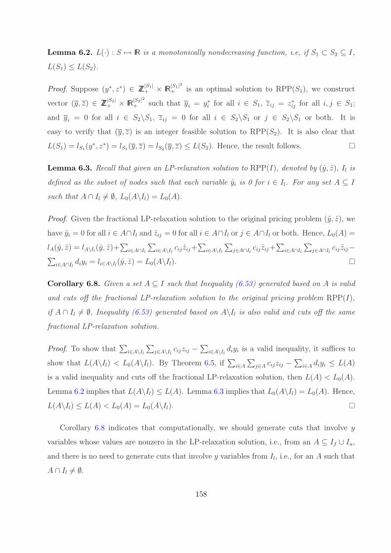
Lemma 6.2. L(·) : S 7→ IR is a monotonically nondecreasing function, i.e, if S1 ⊂ S2 ⊆ I,
L(S1) ≤ L(S2).
Proof. Suppose (y∗, z∗) ∈ ZZ|S1|+ × IR
|S1|2+ is an optimal solution to RPP(S1), we construct
vector (y, z) ∈ ZZ|S2|+ × IR
|S2|2+ such that yi = y∗
i for all i ∈ S1, zij = z∗ij for all i, j ∈ S1;
and yi = 0 for all i ∈ S2\S1, zij = 0 for all i ∈ S2\S1 or j ∈ S2\S1 or both. It is
easy to verify that (y, z) is an integer feasible solution to RPP(S2). It is also clear that
L(S1) = lS1(y∗, z∗) = lS1(y, z) = lS2(y, z) ≤ L(S2). Hence, the result follows.
Lemma 6.3. Recall that given an LP-relaxation solution to RPP(I), denoted by (y, z), Il is
defined as the subset of nodes such that each variable yi is 0 for i ∈ Il. For any set A ⊆ I
such that A ∩ Il 6= ∅, L0(A\Il) = L0(A).
Proof. Given the fractional LP-relaxation solution to the original pricing problem (y, z), we
have yi = 0 for all i ∈ A∩Il and zij = 0 for all i ∈ A∩Il or j ∈ A∩Il or both. Hence, L0(A) =
lA(y, z) = lA\Il(y, z)+
∑
i∈A∩Il
∑
i∈A\Ilcij zij+
∑
i∈A\Il
∑
j∈A∩Ilcij zij+
∑
i∈A∩Il
∑
j∈A∩Ilcij zij−
∑
i∈A∩Ildiyi = li∈A\Il
(y, z) = L0(A\Il).
Corollary 6.8. Given a set A ⊆ I such that Inequality (6.53) generated based on A is valid
and cuts off the fractional LP-relaxation solution to the original pricing problem RPP(I),
if A ∩ Il 6= ∅, Inequality (6.53) generated based on A\Il is also valid and cuts off the same
fractional LP-relaxation solution.
Proof. To show that∑
i∈A\Il
∑
j∈A\Ilcijzij −
∑
i∈A\Ildiyi is a valid inequality, it suffices to
show that L(A\Il) < L0(A\Il). By Theorem 6.5, if∑
i∈A
∑
j∈A cijzij −∑
i∈A diyi ≤ L(A)
is a valid inequality and cuts off the fractional LP-relaxation solution, then L(A) < L0(A).
Lemma 6.2 implies that L(A\Il) ≤ L(A). Lemma 6.3 implies that L0(A\Il) = L0(A). Hence,
L(A\Il) ≤ L(A) < L0(A) = L0(A\Il).
Corollary 6.8 indicates that computationally, we should generate cuts that involve y
variables whose values are nonzero in the LP-relaxation solution, i.e., from an A ⊆ If ∪ Iu,
and there is no need to generate cuts that involve y variables from Il, i.e., for an A such that
A ∩ Il 6= ∅.
158
Remark 6.6. Suppose L(If ) < L0(If ), then the inequality∑
i∈If
∑
j∈Ifcijzij −
∑
i∈Ifdiyi ≤
L(If ) is a valid inequality that cuts off the fractional LP-relaxation solution to RPP(I).
6.2.2.1 A Pure Cutting-Plane Algorithm It is easy to see that any of the above
theoretical results is still valid with slight modification when additional cutting planes are
added to the LP relaxation of RPP. Theorem 6.4 ensures that before reaching optimality, a
cutting plane can always be generated by solving RPP(If ∪ Iu). Hence a pure cutting-plane
algorithmic framework is presented as follows. For ease of exposition, we use Ayy + Azz +
Az0z0 + Auu = b to represent all constraints in the LP relaxation of RPP.
Algorithm 6.1. (A Pure Cutting-Plane Algorithm)
Initialization: Set t = 1, S1R = {l0 ∈ IR
1, (y, z, z0, u) ∈ IR|I|+ × IR
|I|2+ × IR
|I|+ × IR
|I|2/2+ :
l0 − (∑
i∈I
∑
j∈I cijzij −∑
i∈I diyi) = 0, Ayy + Azz + Az0z0 + Auu = b}.
Iteration t:
Step 1: Solution of the LP relaxation. Solve
(RPP LPt) max{l0 : (l0, y, z, z0, u) ∈ StR}.
Suppose the optimal solution of RPP LPt is (lt0, yt, zt, (z0)t, ut). Set I t
f and I tu to be
the sets of yt and zt variables in which the values of yt variables are fractional and
1.
Step 2: Optimality test. If yt ∈ ZZ|I|+ , then yt is part of an optimal solution. Deter-
mine the values of other decision variables. DONE and output the optimal solution.
Otherwise, select At ⊆ If ∪ Iu.
Step 3: Cut generation. If L(At) < L0(At), go to Step 4. Otherwise, go to Step
5.Step 4: Addition of a cut. Set
St+1R = St
R∩
l0 ∈ IR1, (y, z, z0, u) ∈ IR
|I|+ × IR
|I|2+ × IR
|I|+ × IR
|I|2/2+ :
∑
i∈At
∑
j∈At
cijzij −∑
i∈At
diyi ≤ L(At)
.
Go to Step 6.
159

Step 5: Addition of a node subset. At ← At ∪ A, where A ⊆ I and A ∩ At = ∅.
Go to Step 3.
Step 6: Set t← t + 1.
We now show the presented pure cutting-plane algorithm is correct and converges finitely.
Theorem 6.6. Algorithm 6.1 terminates finitely at iteration t where yt is the optimal set of
nodes.
Proof. At each iteration t, Algorithm 6.1 solves RPP(At) finitely many times and obtains the
final optimal objective value L(At) for generating cutting planes. Let us consider the integer
hull of RPP. It is clear that it is [0, 1]|I| since every corner point of the |I|-dimensional binary
hypercube is an integer feasible solution to RPP. By Theorem 6.5, Step 4 of the algorithm
at iteration t obtains an extreme point on the projection of the integer hull onto IR|At|+ . The
projection is the binary hypercube [0, 1]|At|. It thus generates a face of the integer hull of
RPP and the associated cutting plane cuts off all fractional solutions that project into the
hypercube. This also implies that such a cutting plane would not be generated repeatedly.
Hence finite convergence follows from that there are finitely many faces on the integer hull of
RPP. It is easy to see lt0, t = 1, . . . , k, is a decreasing sequence and lt0 ≥ L(I) for all t. The
algorithm terminates when an integer feasible solution is found, then lk0 ≤ L(I). Therefore,
lk0 = L(I).
To summarize, Theorem 6.5 ensures that before reaching optimality, a separating hy-
perplane can always be generated to separate integer feasible solutions and the incumbent
optimal solution to the LP relaxation. The convergence follows from the fact that there
are finitely many faces of the integer hull of RPP that one has to generate before reaching
optimality.
Theorem 6.5 indicates the potential that we could greatly reduce the size of the solved
pricing problem in cut generation to speed up the pricing problem solution. Intuitively,
however, the more y decision variables are excluded when selecting At, the less likely that
a cutting plane of this class indeed exists in the lower-dimensional space induced by At.
This is because it is less likely to satisfy the condition L(At) < L0(At) when |At| is small.
Hence a computational trade-off is presented in size selection of the solved pricing problem.
160
If At is of higher dimension, stronger cuts tend to be generated although each solution of
the pricing problem is more time-consuming; if At is of lower dimension, weaker cuts tend
to be generated although each solution of the pricing problem takes less time. One more
disadvantage of choosing lower-dimensional At is that it may be difficult to find an A such
that L(At) < L0(At). Theorem 6.4 indicates when using a subset of I, If ∪ Iu, the condition
L(If ∪ Iu) < L0(If ∪ Iu) does not need to be checked. In fact, If ∪ Iu is the smallest such
subset of I. It is not clear how to select At. A good starting point may be I tf since it
contains all fractional dimensions in the current LP-relaxation solution. If we start from I tf ,
we may not be able to generate a cutting plane at the beginning. It is not clear which y
variables in Iu should be added to At and what order in which they should be checked. It is
also not clear how to compute L(At). Two options in terms of solving the pricing problem
constructed based on At are: one, solve the problem in a mixed-integer programming solver
after constructing the problem; two, enumerate possible integer solutions (integer solutions
that are neighbor to the projection of the fractional optimal solution onto the space induced
by At) and select the one that gives the largest objective value. Overall, the best algorithmic
choice is not obvious and thus computational investigation is needed, which is left for future
work.
Some preliminary computational experiments show that this pure cutting-plane algo-
rithm tends to require an exorbitant number of cuts. Each cutting plane appears to be not
strong. It is likely that we have to generate a cutting plane in the space induced by I. This
means that one has to solve RPP, which is obviously undesirable.
6.2.2.2 Cut Generation in the Branch-and-Bound Solution (Class II) Similar
to the cut generation of Class I valid inequalities in the branch-and-bound solution, we add
Class II valid inequalities for each node in the branch-and-bound tree where some variables
are already fixed to 0 or 1 and others are still fractional.
At any node of the branch-and-bound tree s, let us define Is0 and Is
1 to be the sets of
variables in RPP that are already fixed to 0 and 1. Let us also define Isf , Is
l , Isu to be the
161

sets of variables whose values are fractional, 0, and 1, in an LP-relaxation to RPP with
restriction of Is0 and Is
1 . Theorem 6.7 shows that a result similar to Theorem 6.4 can be
derived at other nodes in the branch-and-bound tree besides the root node.
Theorem 6.7. Denote RPPs(A) to the pricing problem that is at node s of the branch-and-
bound tree and is constructed by A ⊆ Is := I\(Is0 ∪ Is
1) = Isf ∪ Is
l ∪ Isu. Let Ls(A) be the
optimal objective value of RPPs(A). The following inequality
∑
i∈Isf∪Is
u
∑
j∈Isf∪Is
u
cijzij −∑
i∈Isf∪Is
u
diyi ≤ Ls(Isf ∪ Is
u), (6.54)
is violated by the fractional LP-relaxation solution to the pricing problem RPPs(Is), but
satisfied by all integer feasible solutions to RPPs(Is).
Proof. The proof is the same to that in Theorem 6.4 except that the argument is applied
here for Is := I\(Is0 ∪ Is
1).
Denote Ls0(I
sf∪Is
u) to be the optimal objective value of the LP relaxation of RPPs(Isf∪Is
u).
Note that if Ls(Isf ∪ Is
u) = Ls0(I
sf ∪ Is
u), then node s in the branch-and-bound tree can be
fathomed due to integrality.
Theorem 6.7 presents an inequality that is valid at a particular node of the branch-and-
bound tree. A result similar to Theorem 6.5 can also be derived for any arbitrary set A
once the condition Ls(A) < Ls0(A) is given. Remark 6.7 shows that at any node in the any
branch-and-bound tree, we can also add inequalities that are valid for all nodes in the tree.
Remark 6.7. As defined earlier, L(Isf ∪ Is
u ∪ Is1) is the optimal objective value of RPP(Is
f ∪
Isu ∪ Is
1). The following inequality
∑
i∈Isf∪Is
u∪Is1
∑
j∈Isf∪Is
u∪Is1
cijzij −∑
i∈Isf∪Is
u∪Is1
diyi ≤ L(Isf ∪ Is
u ∪ Is1), (6.55)
is valid for RPP(I).
162
Remark 6.7 is, in fact, a special case of Theorem 6.4. To have Inequality (6.55) cut off
any fractional solution, stronger conditions need to be imposed.
Now let us summarize the two classes of valid inequalities. Both of them may help before
using branch and bound to solve RPP. Both of them may also help within the branch-
and-bound framework. We are, however, unable to draw any sophisticated and decisive
conclusions on algorithmic selection for solving RPP. This leads to a need for comprehensive
computational investigation. Some attempts have been made and preliminary results are
presented in the next section.
6.3 COMPUTATIONAL EXPERIMENTS
Two sets of computational experiments are conducted. In the first set, we study the compu-
tational performance of four theoretically equivalent formulations presented in Section 6.1.
In the second set, we study the strength of valid inequalities in the first class derived in Sec-
tion 6.2. As in Chapter 5.6, we only consider linear as the functional relationship between
primary nonfunction and cold ischemia time in these experiments. We still set the pure
distribution likelihood lij to be pj, the number of patients awaiting transplant at OPO j,
for all i, j ∈ I, the likelihood that an organ procured at donor OPO i is available for MELD
patients at the regional level, βi = 1 for all i ∈ I, and the pure national flow likelihood l0i to
be constant for all i ∈ I. Other coefficient specifications are different from Chapter 5.6 and
will be given later in respective sections.
6.3.1 Alternative Pricing Problem Formulation Comparison
In this set of computational experiments, we construct an instance based on 30 OPOs indexed
by 1 to 30 (see Appendix B). We set l0i = 1000 for all i ∈ I and randomly generate a set
of duals. We solve the four alternative formulations using the CPLEX MIP solver on a PC
with 797MHz Pentium III processor and 256MB of RAM. All the CPLEX parameter settings
are default. We report in Table 27 several measures associated with the CPLEX branch-
163
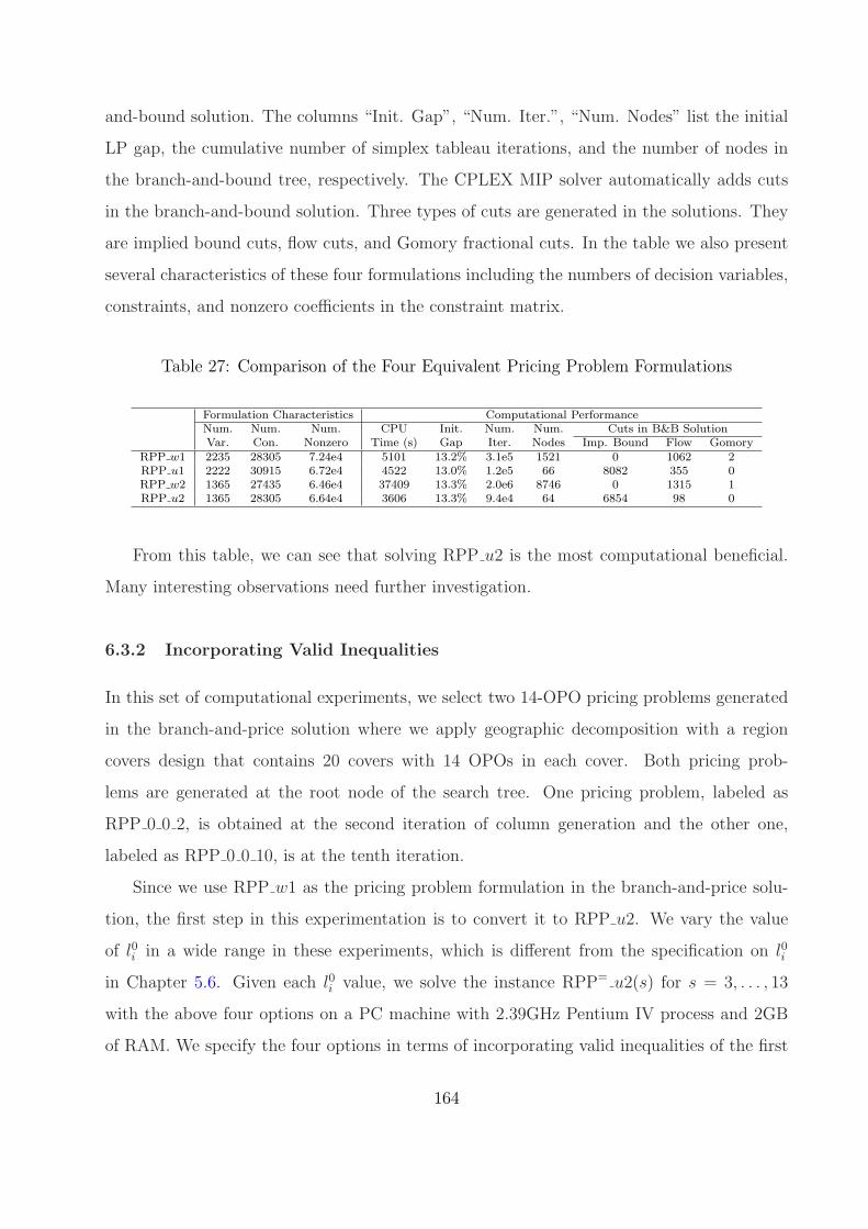
and-bound solution. The columns “Init. Gap”, “Num. Iter.”, “Num. Nodes” list the initial
LP gap, the cumulative number of simplex tableau iterations, and the number of nodes in
the branch-and-bound tree, respectively. The CPLEX MIP solver automatically adds cuts
in the branch-and-bound solution. Three types of cuts are generated in the solutions. They
are implied bound cuts, flow cuts, and Gomory fractional cuts. In the table we also present
several characteristics of these four formulations including the numbers of decision variables,
constraints, and nonzero coefficients in the constraint matrix.
Table 27: Comparison of the Four Equivalent Pricing Problem Formulations
Formulation Characteristics Computational PerformanceNum. Num. Num. CPU Init. Num. Num. Cuts in B&B SolutionVar. Con. Nonzero Time (s) Gap Iter. Nodes Imp. Bound Flow Gomory
RPP w1 2235 28305 7.24e4 5101 13.2% 3.1e5 1521 0 1062 2RPP u1 2222 30915 6.72e4 4522 13.0% 1.2e5 66 8082 355 0RPP w2 1365 27435 6.46e4 37409 13.3% 2.0e6 8746 0 1315 1RPP u2 1365 28305 6.64e4 3606 13.3% 9.4e4 64 6854 98 0
From this table, we can see that solving RPP u2 is the most computational beneficial.
Many interesting observations need further investigation.
6.3.2 Incorporating Valid Inequalities
In this set of computational experiments, we select two 14-OPO pricing problems generated
in the branch-and-price solution where we apply geographic decomposition with a region
covers design that contains 20 covers with 14 OPOs in each cover. Both pricing prob-
lems are generated at the root node of the search tree. One pricing problem, labeled as
RPP 0 0 2, is obtained at the second iteration of column generation and the other one,
labeled as RPP 0 0 10, is at the tenth iteration.
Since we use RPP w1 as the pricing problem formulation in the branch-and-price solu-
tion, the first step in this experimentation is to convert it to RPP u2. We vary the value
of l0i in a wide range in these experiments, which is different from the specification on l0i
in Chapter 5.6. Given each l0i value, we solve the instance RPP= u2(s) for s = 3, . . . , 13
with the above four options on a PC machine with 2.39GHz Pentium IV process and 2GB
of RAM. We specify the four options in terms of incorporating valid inequalities of the first
164

Table 28: Strength of Class I Valid Inequalities (RPP 0 0 2)
National Cardinality LP Duality Gap (%) CPU Time (s)Flow li0 Value O1 O2 O3 O4 O1 O2 O3 O4
3 68.2 39.6 32.9 19.7 2.67 0.87 2.43 1.114 47.2 24.8 15.8 10.7 2.50 1.57 1.89 1.425 40.4 20.9 11.7 9.5 2.62 1.48 2.14 0.956 40.7 22.2 11.7 9.7 2.88 3.09 2.43 2.167 39.2 21.8 11.4 9.6 4.25 2.57 3.42 3.31
1000 8 38.0 21.0 11.2 9.1 4.86 5.24 3.27 4.469 37.3 20.2 11.3 8.7 5.57 5.64 3.17 3.4110 36.3 18.0 10.8 8.2 6.19 5.21 3.05 3.5111 22.5 10.6 5.3 2.9 0.74 1.28 1.76 0.9612 38.8 11.7 2.5 2.0 0.60 1.65 0.40 0.7213 133.3 19.9 3.2 2.8 0.86 0.78 0.44 1.123 40.3 31.9 24.1 18.3 1.68 0.97 1.94 1.074 25.0 19.5 10.0 7.8 1.71 1.32 1.42 1.455 20.3 15.4 7.0 6.4 2.62 2.57 2.22 0.656 21.0 15.3 7.0 6.4 2.88 5.46 3.02 1.717 20.1 14.5 6.7 6.1 4.25 5.21 3.45 2.74
500 8 19.3 13.1 6.6 5.8 4.86 5.80 2.78 4.949 18.9 12.1 6.5 5.6 5.57 5.60 3.32 5.1810 18.4 11.0 6.2 5.0 6.19 6.00 3.75 5.2911 6.8 1.6 1.6 0.5 0.74 1.86 0.75 1.7012 12.9 0.9 1.0 0.6 0.60 3.45 0.35 1.7513 40.1 1.0 1.0 0.8 0.86 3.71 1.83 1.473 28.2 25.0 19.1 16.1 1.41 1.43 1.23 1.224 15.7 12.3 6.9 5.2 1.39 1.44 1.31 0.425 11.9 8.7 4.5 4.0 1.89 1.40 1.51 0.816 12.8 8.7 4.6 4.0 2.05 2.07 1.77 1.657 12.3 8.3 4.4 3.8 2.47 1.85 2.06 3.32
300 8 11.7 7.4 4.2 3.6 3.26 2.04 1.70 2.169 11.4 6.8 4.2 3.3 2.79 2.04 2.42 1.9910 11.0 6.1 3.9 3.0 2.86 2.47 2.48 3.0111 0.5 0.0 0.0 0.0 0.73 0.55 0.38 0.5912 3.9 0.1 0.4 0.0 0.42 0.95 0.39 0.5013 18.1 0.3 0.5 0.3 1.27 0.97 0.54 0.76
class. Option “O1” is not adding any valid inequalities. Option “O2” is adding all valid
inequalities associated with variables z and u in (6.46) and (6.47). Option “O3” is adding
all valid inequalities associated with variables z0 and u in (6.48). Option “O4” is adding
all valid inequality from Options 2 and 3. With each option, we record the CPU time and
duality gap and report the results in Tables 28 and 29.
165

Table 29: Strength of Class I Valid Inequalities (RPP 0 0 10; only consider CPU time)
National Cardinality ValueFlow li0 Option 3 4 5 6 7 8 9 10 11 12 13
O1 7.7 27.2 42.1 47.1 38.9 30.0 30.1 30.8 33.1 30.8 24.6O2 7.0 14.9 31.3 56.8 75.7 62.1 56.9 36.3 32.4 27.5 14.8
1000 O3 17.2 18.8 24.7 19.6 27.0 21.5 27.6 24.5 22.3 19.3 11.9O4 4.2 10.3 10.4 16.3 23.2 20.7 22.1 19.3 22.1 15.6 10.3O1 7.9 26.9 39.8 54.4 70.8 67.9 57.2 48.7 42.1 31.4 21.4O2 8.2 34.4 27.6 160.7 187.9 75.0 66.5 52.6 36.6 28.6 18.8
500 O3 18.7 26.4 40.9 53.5 67.2 57.5 115.1 50.0 27.7 23.3 11.3O4 10.1 15.0 25.4 31.0 27.6 49.8 55.8 39.8 25.3 17.1 14.16O1 7.9 25.7 56.3 73.1 124.1 65.1 45.9 51.2 46.7 37.1 24.5O2 8.7 21.7 68.3 123.7 169.8 109.3 77.8 58.7 50.6 35.8 22.2
300 O3 13.3 37.3 52.9 66.6 56.7 74.9 60.1 51.3 25.4 20.8 11.9O4 17.5 30.5 54.6 66.8 54.9 133.3 79.3 75.2 44.7 21.3 12.8
The reason that Table 29 only presents CPU times is because the optimal objective
value to pricing problem RPP 0 0 10 is close to 0 and thus the optimal objective value to
its LP relaxation is potentially negative. As a result, the initial duality gap is usually big or
negative. Therefore, we do not consider it in this case.
Several observations are made in this set of experiments. First, it is intuitive that the
pricing problem becomes harder to solve as the solution applying column generation proceeds.
This is verified by comparing the results in Tables 28 and 29. Second, Table 28 clearly
indicates that Option 1 results in the least tight formulation among the four whereas Option
4 leads to the tightest one. This is a desirable observation since the formulation associated
with Option 4 is obtained by adding all Class I valid inequalities. A similar observation is
unlikely made in terms of the CPU time. In general, Option 4 provides the least CPU time
in more cases than any other option. However, Option 4 cannot be considered as a dominant
option. Another observation is made when comparing Options 2 and 3. The results in both
tables suggest that Option 3 tends to be preferable as l0i decreases or the cardinality value
increases and Option 2 tends to be preferable when the opposite condition holds. This
preference reflects on both formulation tightness and solution time.
166

Figure 29: Illustration of Unimodality (l0i = 1000, 500, and 300)
We also test other l0i values. They are 1, 2, 3, 5, 10, 20, 30, 50, 100, and 200. We include
the related computational results in several tables similar to Tables 28 and 29 in Appendix
G. A comparison of computational results associated with various l0i values suggests that it
is less likely to be clear which option is the best choice as the value of l0i deceases.
Figure 29 shows the optimal objective value of RPP=(s) as a function of the cardinality
value s. Note that the instance is RPP 0 0 2. First, the figure indicates that when s is fixed,
the optimal objective value decreases as l0i increases. It strongly argues that this decrease is
monotonic. Second, the figure shows that for all three l0i values, unimodality holds in terms
of the relationship between the optimal objective value of RPP=(s) and the cardinality value
s. As s increases, the optimal objective value first increases and then decreases. A few more
figures that are included in Appendix H further suggest that the relationship, in general,
tends to be unimodal or monotonically nondecreasing or monotonically nonincreasing, for
RPP=(s). This observation confirms the applicability of the three algorithmic approaches
to finding the optimal set cardinality in the pricing problem of our region design problem.
167
7.0 PROPORTIONAL ALLOCATION GENERALIZATION
As we have presented in Chapters 4 and 5, the estimate of the regional benefit for each
potential region is based on the proportional allocation scheme. In this chapter, we attempt
to generalize the estimation along the direction of conducting the allocation through multiple
steps, at each of which proportional allocation is imposed.
7.1 INTRODUCTION
Let us describe organ allocation in a more general way. Once an organ is procured at a
procurement site, it is proportionally allocated to various recipient sites, and thus a benefit
of the procured organ occur. For the objective function coefficient estimate in our region
design problem, the benefit of an individual organ is dependent upon the geographic dis-
tance between the procurement and recipient sites. We call this benefit an individual-organ
benefit. The regional benefit is obtained by accumulating the individual-organ benefit over
all procured organs in the region. So it is also dependent upon the allocation quantity of
organs besides the factor affecting the individual-organ benefit. In organ allocation, organs
are allocated to patients proportionally and then transplants occurs. Therefore, it is one-step
allocation. A natural way to generalize the estimate is to consider there are multiple steps
through the allocation process. When considering the likelihood of allocation at each step,
the proportional allocation scheme is still imposed.
168

7.1.1 Generic Set-Partitioning Formulation
Since we only attempt to generalize the estimate of the regional benefit, the set-partitioning
formulation does not change. Here we first present a generic set-partitioning formulation.
Given a set I, one can construct the set containing all subsets of I that should be
considered. Let us denote this set to be A. Note that A may not contain all possible subsets
of I given some restriction. For instance, in Stahl et al. [195], we defined the problem on
a graph G = (I, E) and only considered connected subgraphs given the node-arc adjacency
matrix of the graph that indicates adjacency of any two OPOs. Let us define c(A) for A ∈ A
to be the benefit function induced by A, i.e., c(·) : S 7→ IR. Let us also define ai,A = 1 if
i ∈ A; 0, otherwise.
Then the generic set-partitioning formulation is presented as:
max
{
∑
A∈Ac(A)xA
∑
A∈Aai,AxA = 1,∀i ∈ I; xA ∈ IB,∀A ∈ A
}
. (7.1)
7.1.2 Grouping Quantity Generalization
In this section, we discuss the essence of the proportional allocation generalization. Let us
first introduce several relevant concepts. Suppose there are K commodities associated with
each procurement site i (we use “node” in the following presentation) and the procurement
quantity of each commodity is known as qki for i ∈ I and 1 ≤ k ≤ K.
In a commodity matching network, various commodities at different nodes are grouped in
the subnetwork induced by these nodes. This action can be done by matching in various real-
world settings. For example, in the organ transplantation and allocation network, there are
two commodities, organ and patient. One physical interpretation of grouping is that organs
and patients are matched between two OPOs, the procurement OPO and the recipient OPO.
Let us define a pair of K-tuples Tδ = (δ1, δ2, . . . , δK) and Ti = (i1, i2, . . . , iK) to represent
the matching motivated above. Such a pair indicates that the group comprises commodity
δ1 from node i1, commodity δ2 from node i2, up to commodity δK from node iK . We call
such a grouping a K-grouping. In Figure 30, there are four commodities and three nodes.
K = 4 and two 4-groupings are specified. They are T 1δ = (1, 2, 3, 4) and T 1
i = (1, 1, 2, 1), and
169
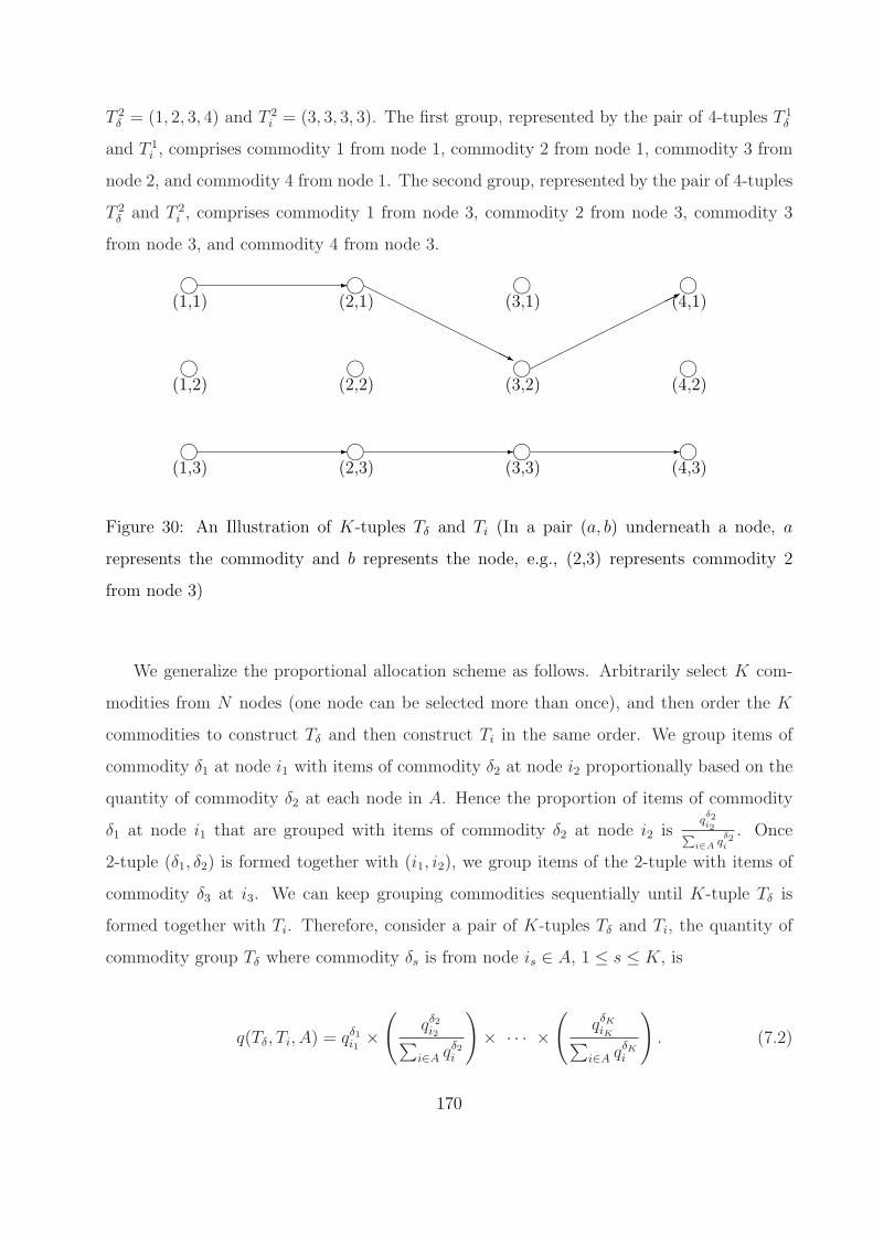
T 2δ = (1, 2, 3, 4) and T 2
i = (3, 3, 3, 3). The first group, represented by the pair of 4-tuples T 1δ
and T 1i , comprises commodity 1 from node 1, commodity 2 from node 1, commodity 3 from
node 2, and commodity 4 from node 1. The second group, represented by the pair of 4-tuples
T 2δ and T 2
i , comprises commodity 1 from node 3, commodity 2 from node 3, commodity 3
from node 3, and commodity 4 from node 3.
j
j
j
j
j
j
j
j
j
j
j
j- HHHHHHHHHHHj �����������*
- - -
(1,1)
(1,2)
(1,3)
(2,1)
(2,2)
(2,3)
(3,1)
(3,2)
(3,3)
(4,1)
(4,2)
(4,3)
Figure 30: An Illustration of K-tuples Tδ and Ti (In a pair (a, b) underneath a node, a
represents the commodity and b represents the node, e.g., (2,3) represents commodity 2
from node 3)
We generalize the proportional allocation scheme as follows. Arbitrarily select K com-
modities from N nodes (one node can be selected more than once), and then order the K
commodities to construct Tδ and then construct Ti in the same order. We group items of
commodity δ1 at node i1 with items of commodity δ2 at node i2 proportionally based on the
quantity of commodity δ2 at each node in A. Hence the proportion of items of commodity
δ1 at node i1 that are grouped with items of commodity δ2 at node i2 isq
δ2i2
P
i∈A qδ2i
. Once
2-tuple (δ1, δ2) is formed together with (i1, i2), we group items of the 2-tuple with items of
commodity δ3 at i3. We can keep grouping commodities sequentially until K-tuple Tδ is
formed together with Ti. Therefore, consider a pair of K-tuples Tδ and Ti, the quantity of
commodity group Tδ where commodity δs is from node is ∈ A, 1 ≤ s ≤ K, is
q(Tδ, Ti, A) = qδ1i1×
(
qδ2i2
∑
i∈A qδ2i
)
× · · · ×
(
qδK
iK∑
i∈A qδK
i
)
. (7.2)
170

j
j
j
j
j
j
j
j
j
j
j
j
- - -
- - -
- - -
�����������*
�����������*
�����������*�����������*
�����������*
�����������*
HHHHHHHHHHHj
HHHHHHHHHHHj
HHHHHHHHHHHj
HHHHHHHHHHHj
HHHHHHHHHHHj
HHHHHHHHHHHj
@@
@@
@@
@@
@@
@R
@@
@@
@@
@@
@@
@R
@@
@@
@@
@@
@@
@R��
��
��
��
��
��
��
��
��
��
��
��
��
��
��
��
��
��(1,1)
(1,2)
(1,3)
(2,1)
(2,2)
(2,3)
(3,1)
(3,2)
(3,3)
(4,1)
(4,2)
(4,3)
q11
q12
q13
q21
q22
q23
q31
(q32
q33
q41
q42
q43
q11·
q21
q21+q2
2+q23
q11·
q23
q21+q2
2+q23
q11·
q21
q21+q2
2+q23·
q31
q21+q2
2+q23
Figure 31: Illustration of Proportional Allocation in K-grouping
We generalize the calculation of grouping quantity through a list of nodes in a subnetwork
in (7.2). Figure 31 illustrates the grouping process. For example, we can see in the figure
that commodity 1 at node 1 is proportionally allocated to nodes 1, 2, and 3. Therefore, the
quantity of commodity 1 at node 1 grouped with commodity 2 at node 1 is q11 ·
q21
q21+q2
2+q23
and
the quantity of commodity 1 at node 1 grouped with commodity 2 at node 3 is q11 ·
q23
q21+q2
2+q23.
Here is another example. If Tδ = (1, 2, 3, 4), Ti = (1, 1, 1, 1), and A = {1, 2, 3}, then
q(Tδ, Ti, A) = q11 ·
q21
q21 + q2
2 + q23
·q31
q31 + q3
2 + q33
·q41
q41 + q4
2 + q43
.
The first two steps of the grouping process are illustrated on Figure 31.
Now let us focus on the allocation at one step in the grouping process. Suppose we have
grouped the first s commodities in Tδ. It is easy to see that the quantity of this s-commodity
group at node is ∈ A is
qs(is) =∑
i1∈A
∑
i2∈A
· · ·∑
is−1∈A
qδ1i1×
(
qδ2i2
∑
i∈A qδ2i
)
× · · · ×
(
qδs
is∑
i∈A qδs
i
)
.
The items of the s-commodity group are then proportionally grouped with the (s + 1)th
commodity in Tδ to form a (s + 1)-commodity group. An implicitly stated condition here
is that all items of the s-commodity group are able to find matches at this step. In other
words, the (s + 1)th commodity is abundant relative to the s-commodity group in the sense
that the quantity of the (s + 1)th commodity at any node is greater than or equal to the
171

allocation quantity of the s-commodity group to that node. Mathematically, it is presented
as: qs+1i ≥
∑
j∈A qs(j) ·q
δs+1i
P
k∈A qδs+1k
= qs+1(i) for all i ∈ A. This condition needs to hold at
each step of the grouping process. If we view the first s components in Ti as a supplier and
the (s + 1)th component as a client, the condition implies that demand exceeds supply to
every client in this supply-demand setting. Note that due to the fact that organs are scarce
resources, it is the case in the organ transplantation and allocation network, in which organs
are commodity 1 and patients are commodity 2.
Now we are ready to discuss the generalized regional benefit estimation. Let us assume
that all grouping items based on a pair of K-tuples Tδ and Ti, namely following the same
lists of commodities and nodes in the subnetwork, are identical in terms of benefit generation
and call the benefit generated by an individual grouping item the individual-group benefit,
denoted as α(Tδ, Ti, A). Note that one should know the list of commodities Tδ beforehand.
We also assume that the regional benefit given Tδ is obtained in an additive manner. That
is, it is simply the sum of the individual-group benefit over all grouping items, i.e.,
c(A) =∑
Ti∈Ti
c(Tδ, Ti, A) =∑
Ti∈Ti
q(Tδ, Ti, A) · α(Tδ, Ti, A), (7.3)
where Ti is the set containing all possible K-tuples chosen from A with replacement. Here
the regional benefit c(A) should be represented as c(A, Tδ), which is dependent upon the
commodity list. Since as mentioned earlier, the commodity list is known a priori, we drop
Tδ in the exposition. More discussion on the order of commodity grouping appears later in
this section.
Now let us specify (7.3) by substituting (7.2) in and assuming the individual-group benefit
is only dependent upon the node list, i.e., α(Tδ, Ti, A) = α(Ti). Then the regional benefit
c(A) =
∑
i1∈A
∑
i2∈A
· · ·∑
iK∈A
qδ1i1×
(
qδ2i2
∑
i∈A qδ2i
)
× · · · ×
(
qδK
iK∑
i∈A qδK
i
)
× α(i1, i2, . . . , iK). (7.4)
Previously, we state that one should know the list of commodities, Tδ, beforehand. Now
let us discuss the effect of different lists of commodities. We will construct an example as
follows to show different Tδ cause different regional benefits and different optimal regional
172

configurations obtained by solving the set-partitioning problem. Suppose we consider a 2-
node network with 2 commodities. The input parameters are (q11, q
12, q
21, q
22) = (1, 1, 1, 2) and
(α11, α12, α21, α22) = (43, 1, 2
3, 1
3). Note that α(Tδ, Ti, A) is assumed to be independent of Tδ
and αij = α(i, j). There are only two regional configurations: two nodes in the same region
or two nodes in different regions, i.e., {1, 2} and {{1}, {2}}. In the case where Tδ = (1, 2),
c({1, 2}) = 149
and c({1}) + c({2}) = 53. In the case where Tδ = (2, 1), c({1, 2}) = 13
6and
c({1}) + c({2}) = 2. Thus {{1}, {2}} is the optimal configuration when Tδ = (1, 2), whereas
{1, 2} is the optimal configuration when Tδ = (2, 1).
7.1.3 An Alternative Interpretation of the Generalization
Earlier in this section, we provide an interpretation of the generalization during its derivation.
That is, multiple commodities are grouped based on the proportional allocation scheme. We
present an alternative interpretation in the following.
In a single commodity sharing network, items of the commodity are distributed through
a channel that consists of a set of nodes A. This distribution is proportional based on the
value of an attribute associated with each step. Therefore, we replace the K-tuple Tδ with
Ta = (a1, a2, . . . , aK−1), a (K − 1)-tuple representing a list of attributes. Arbitrarily select
a list of nodes Ti and a list of attributes Ta. In the first step, we distribute qi1 items of the
commodity at node i1 proportionally to all nodes in A based on the value of attribute a1 at
each node. In step s, we distribute items of the commodity at one node to all nodes in A
based on the value of attribute as. After K − 1 steps, the distribution process is completed.
Define qi1 to be the initial quantity of the commodity at node i1. Define vas
is+1to be the value
of the attribute associated with step s at node is+1, s = 1, . . . K − 1. We present a formula
similar to (7.2) to calculate the distribution quantity as:
q(Ta, Ti, A) = qi1 ·
(
va1i2
∑
i∈A va1i
)
· · · · ·
(
vaK−1
iK∑
i∈A vaK−1
i
)
. (7.5)
7.1.4 Organ Allocation as an Example
In Stahl et al. [195], we considered a pair of 2-tuples (o, p) and (i1, i2), where i1 is the procure-
ment OPO and i2 is the recipient OPO. Hence, we considered two commodities, organ as com-
173

modity 1 and patient as commodity 2. We captured the effect of organ transport distance on
organ quality decay, and let α(i, j) = αij, which is only dependent upon the distance between
OPOs i and j and independent of the selected region. We also neglected intra-OPO trans-
plantation. Thus we can specify αii = 0 for all i ∈ I in the generalized estimation. Therefore,
the regional benefit c(A) =∑
i∈A
∑
j∈A qoi ·
qpj
P
k∈A qpk
·α(i, j) =∑
i∈A
∑
j∈A\{i} oi ·pj
P
k∈A\{i} pk·αij.
Following the alternative interpretation in Section 7.1.3, organs, as the commodity, are
distributed proportionally from procurement OPOs to recipient OPOs based on the value
of an attribute, patient population in Chapter 3, and pure distribution likelihood and pure
national flow likelihood in following chapters.
7.1.5 1-Commodity Case
At the end of this section, let us consider a special case where neither interpretation applies
since matching/distribution does not occur. We call it the 1-commodity case. The generic
set-partitioning problem can be formulated as:
max∑
A∈A
∑
i∈A
qiα(i, A)xA (7.6)
subject to∑
A∈Aai,AxA = 1,∀i ∈ I; (7.7)
xA ∈ IB,∀A ∈ A. (7.8)
In (7.6), we use qi, the original quantity at each node since no distribution occurs. If we
assume α(i, A) = α(i) as in (7.4), any regional configuration is an optimal solution and thus
the problem becomes trivial.
In the remainder of this chapter, we assume that the individual-group benefit is only
dependent upon the node list, i.e, α(Tδ, Ti, A) = α(Ti) = α(i1,i2,...,iK). Throughout the expo-
sition, we only follow the first interpretation. We will discuss how to solve the generalized
set-partitioning problem. Our approach is to explore the possibility of generalizing the col-
umn generation method discussed earlier for solving our region design problem and put
174

emphasis on the generalized pricing problem. The remainder is organized as follows: Section
7.2 first discusses how to adapt column generation in two special cases and then general-
izes the column generation procedure. We mainly discuss the generalization of the pricing
problem. Section 7.3 generalizes the first class of valid inequalities presented in Chapter 6.
7.2 GENERALIZATION OF THE COLUMN GENERATION APPROACH
Once the regional benefits c(A) are computed for all A ∈ A, one can construct and solve
the set-partitioning problem to obtain the optimal partition directly with an MIP solver.
However, the set-partitioning problem with the generalized regional benefit estimate has
potentially an enormous number of columns. Therefore, we develop a generalization of the
column generation method presented in Chapter 5. Before presenting the generalization,
let us first discuss two special cases, the 2-commodity grouping case and the 3-commodity
grouping case.
7.2.1 2-Commodity Grouping Case
In the 2-commodity grouping case, we want to group two commodities in the only step of
the grouping process based on proportional allocation. The set-partitioning problem can be
formulated as:
max∑
A∈A
(
∑
i∈A
∑
j∈A
qδ1i ·
qδ2j
∑
k∈A qδ2k
· αij
)
· xA (7.9)
subject to
(7.7), (7.8).
Clearly, our region design problem is a 2-commodity grouping problem. Now let us
discuss the application of column generation in this special case. Given π, the dual obtained
by solving the restricted master problem, the associated pricing problem is:
RPP NLP(π) : max
{
∑
i∈I
∑
j∈I
qδ1i yi ·
qδ2j yj
∑
k∈I qδ2k yk
· αij −∑
i∈I
πiyi yi ∈ IB,∀i ∈ I
}
. (7.10)
175
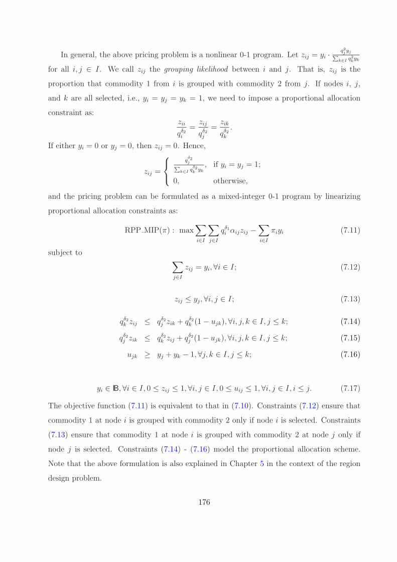
In general, the above pricing problem is a nonlinear 0-1 program. Let zij = yi ·q2j yj
P
k∈I q2kyk
for all i, j ∈ I. We call zij the grouping likelihood between i and j. That is, zij is the
proportion that commodity 1 from i is grouped with commodity 2 from j. If nodes i, j,
and k are all selected, i.e., yi = yj = yk = 1, we need to impose a proportional allocation
constraint as:zii
qδ2i
=zij
qδ2j
=zik
qδ2k
.
If either yi = 0 or yj = 0, then zij = 0. Hence,
zij =
qδ2j
P
k∈I qδ2k
yk
, if yi = yj = 1;
0, otherwise,
and the pricing problem can be formulated as a mixed-integer 0-1 program by linearizing
proportional allocation constraints as:
RPP MIP(π) : max∑
i∈I
∑
j∈I
qδ1i αijzij −
∑
i∈I
πiyi (7.11)
subject to∑
j∈I
zij = yi,∀i ∈ I; (7.12)
zij ≤ yj,∀i, j ∈ I; (7.13)
qδ2k zij ≤ qδ2
j zik + qδ2k (1− ujk),∀i, j, k ∈ I, j ≤ k; (7.14)
qδ2j zik ≤ qδ2
k zij + qδ2j (1− ujk),∀i, j, k ∈ I, j ≤ k; (7.15)
ujk ≥ yj + yk − 1,∀j, k ∈ I, j ≤ k; (7.16)
yi ∈ IB,∀i ∈ I, 0 ≤ zij ≤ 1,∀i, j ∈ I, 0 ≤ uij ≤ 1,∀i, j ∈ I, i ≤ j. (7.17)
The objective function (7.11) is equivalent to that in (7.10). Constraints (7.12) ensure that
commodity 1 at node i is grouped with commodity 2 only if node i is selected. Constraints
(7.13) ensure that commodity 1 at node i is grouped with commodity 2 at node j only if
node j is selected. Constraints (7.14) - (7.16) model the proportional allocation scheme.
Note that the above formulation is also explained in Chapter 5 in the context of the region
design problem.
176

7.2.2 3-Commodity Grouping Case
In the 3-commodity grouping case, we want to group three commodities in two steps of the
grouping process based on proportional distribution. The set-partitioning problem can be
formulated as:
max∑
A∈A
(
∑
i∈A
∑
j∈A
∑
k∈A
qδ1i ·
qδ2j
∑
m∈A qδ2m
·qδ3k
∑
n∈A qδ3n
· αijk
)
· xA (7.18)
subject to
(7.7), (7.8).
Given the dual π, the nonlinear 0-1 pricing problem is presented as:
RPP NLP(π) : max
{
∑
i∈I
∑
j∈I
∑
k∈I
qδ1i yi ·
qδ2j yj
∑
m∈I qδ2mym
·qδ3k yk
∑
n∈I qδ3n yn
· αijk −∑
i∈I
πiyi yi ∈ IB,∀i ∈ I
}
.
(7.19)
Let zij = yi ·q
δ2j yj
P
m∈I qδ2m ym
for all i, j ∈ I and zijk = yi ·q
δ2j yj
P
m∈I qδ2m ym
·q
δ3k
ykP
n∈I qδ3n yn
for all i, j, k ∈ I.
We call zij the first one-step grouping likelihood between i and j, and zijk the first two-
step grouping likelihood between (i, j) and k. Note that zijk = zij ·q
δ3k
ykP
n∈I qδ3n yn
. This can be
interpreted as follows. After forming the commodity group (1,2), we focus on some items
of this commodity group where commodity 1 is from node i and commodity 2 is from node
j. We then group these items with commodity 3 based on the set of quantities qδ3 . We can
thus define yj ·q
δ3k
ykP
n∈I qδ3n yn
as the second one-step grouping likelihood. It differs from the first
one-step grouping likelihood in that the proportional allocation constraint imposed here is
based on a different set of quantities. If nodes i, j, k, m, n are all selected, we need to
impose a proportional allocation constraint at each step of the grouping process as:
zij
qδ2j
=zik
qδ2k
andzijm
qδ3m
=zijn
qδ3n
.
177

If either yi = 0 or yj = 0, then zij = 0. If either zij = 0 or yk = 0, then zijk = 0. Hence,
zij =
qδ2j
P
k∈I qδ2k
yk
, if yi = yj = 1;
0, otherwise,
and
zijk =
qδ2j
P
m∈I qδ2m ym
·q
δ3k
P
n∈I qδ3n yn
, if yi = yj = yk = 1;
0, otherwise.
Therefore, we can alternatively develop a mixed-integer 0-1 program as:
RPP MIP(π) : max∑
i∈I
∑
j∈I
∑
k∈I
qδ1i αijkzijk −
∑
i∈I
πiyi (7.20)
subject to∑
j∈I
zij = yi,∀i ∈ I; (7.21)
zij ≤ yj,∀i, j ∈ I; (7.22)
∑
k∈I
zijk = zij,∀i, j ∈ I; (7.23)
zijk ≤ yk,∀i, j, k ∈ I; (7.24)
qδ2k zij ≤ qδ2
j zik + qδ2k (1− ujk),∀i, j, k ∈ I, j ≤ k; (7.25)
qδ2j zik ≤ qδ2
k zij + qδ2j (1− ujk),∀i, j, k ∈ I, j ≤ k; (7.26)
qδ3n zijm ≤ qδ3
mzijn + qδ3n (1− umn),∀i, j,m, n ∈ I,m ≤ n; (7.27)
qδ3mzijn ≤ qδ3
n zijm + qδ3m(1− umn),∀i, j,m, n ∈ I,m ≤ n; (7.28)
ujk ≥ yj + yk − 1,∀j, k ∈ I, j ≤ k; (7.29)
yi ∈ IB,∀i ∈ I, 0 ≤ zij, zijk ≤ 1,∀i, j, k ∈ I, 0 ≤ uij ≤ 1,∀i, j ∈ I, i ≤ j. (7.30)
178
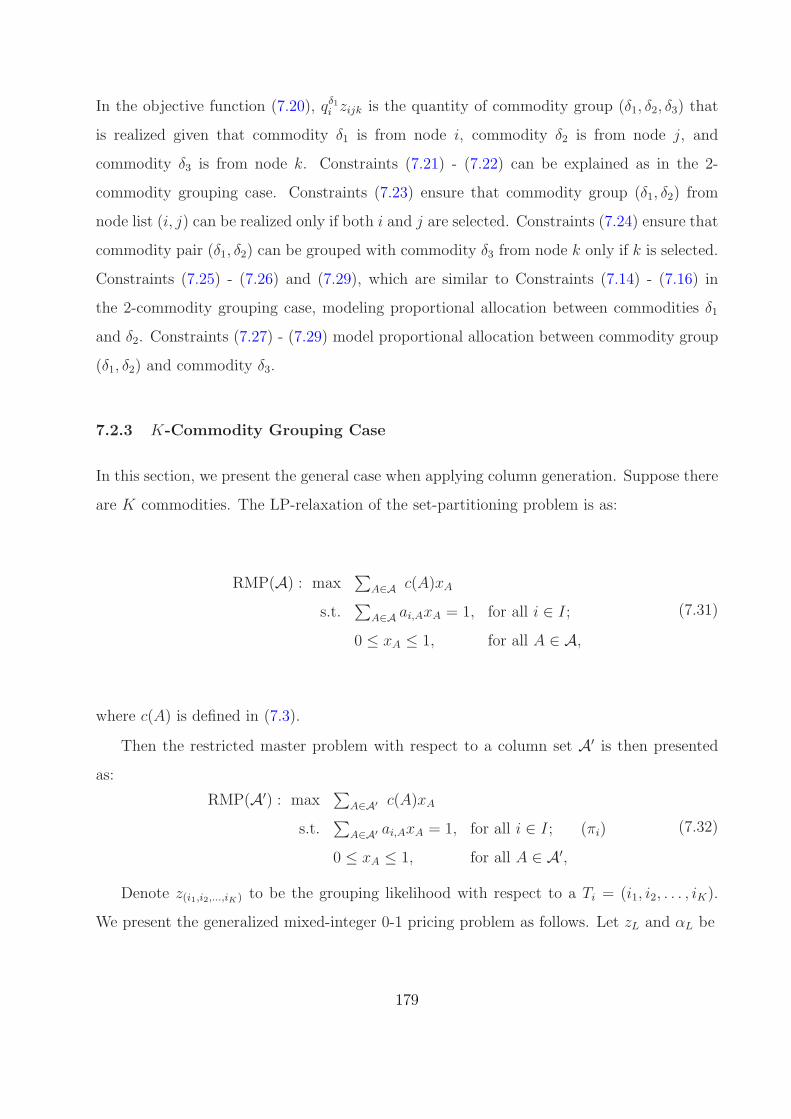
In the objective function (7.20), qδ1i zijk is the quantity of commodity group (δ1, δ2, δ3) that
is realized given that commodity δ1 is from node i, commodity δ2 is from node j, and
commodity δ3 is from node k. Constraints (7.21) - (7.22) can be explained as in the 2-
commodity grouping case. Constraints (7.23) ensure that commodity group (δ1, δ2) from
node list (i, j) can be realized only if both i and j are selected. Constraints (7.24) ensure that
commodity pair (δ1, δ2) can be grouped with commodity δ3 from node k only if k is selected.
Constraints (7.25) - (7.26) and (7.29), which are similar to Constraints (7.14) - (7.16) in
the 2-commodity grouping case, modeling proportional allocation between commodities δ1
and δ2. Constraints (7.27) - (7.29) model proportional allocation between commodity group
(δ1, δ2) and commodity δ3.
7.2.3 K-Commodity Grouping Case
In this section, we present the general case when applying column generation. Suppose there
are K commodities. The LP-relaxation of the set-partitioning problem is as:
RMP(A) : max∑
A∈A c(A)xA
s.t.∑
A∈A ai,AxA = 1, for all i ∈ I;
0 ≤ xA ≤ 1, for all A ∈ A,
(7.31)
where c(A) is defined in (7.3).
Then the restricted master problem with respect to a column set A′ is then presented
as:
RMP(A′) : max∑
A∈A′ c(A)xA
s.t.∑
A∈A′ ai,AxA = 1, for all i ∈ I; (πi)
0 ≤ xA ≤ 1, for all A ∈ A′,
(7.32)
Denote z(i1,i2,...,iK) to be the grouping likelihood with respect to a Ti = (i1, i2, . . . , iK).
We present the generalized mixed-integer 0-1 pricing problem as follows. Let zL and αL be
179

the shorthand notations of z(i1,i2,...,iK) and α(i1,i2,...,iK) in the following formulation. We also
let zL\{iK} = z(i1,i2,...,iK−1), the first (K − 1)-step grouping likelihood with respect to the
partial node list (i1, i2, . . . , iK−1).
GRPP(π) : max∑
i1∈I
∑
i2∈I
· · ·∑
iK∈I
qδ1i1
αLzL −∑
i∈I
πiyi (7.33)
subject to∑
i2∈I
z(i1,i2) = yi1 ,∀i1 ∈ I; (7.34)
z(i1,i2) ≤ yi2 ,∀i1, i2 ∈ I; (7.35)
∑
i3∈I
z(i1,i2,i3) = z(i1,i2),∀i1, i2 ∈ I; (7.36)
z(i1,i2,i3) ≤ yi3 ,∀i1, i2, i3 ∈ I; (7.37)
...
∑
iK∈I
zL = zL\{iK},∀i1, i2, . . . , iK−1 ∈ I; (7.38)
zL ≤ yiK ,∀i1, i2, . . . , iK ∈ I; (7.39)
qδ2k z(i1,j) ≤ qδ2
j z(i1,k) + qδ2k (1− ujk),∀i1, j, k ∈ I, j ≤ k; (7.40)
qδ2j z(i1,k) ≤ pδ2
k z(i1,j) + qδ2j (1− ujk),∀i1, j, k ∈ I, j ≤ k; (7.41)
qδ3k z(i1,i2,j) ≤ qδ3
j z(i1,i2,k) + qδ3k (1− ujk),∀i1, i2, j, k ∈ I, j ≤ k; (7.42)
qδ3j z(i1,i2,k) ≤ qδ3
k z(i1,i2,j) + qδ3j (1− ujk),∀i1, i2, j, k ∈ I, j ≤ k; (7.43)
...
qδK
k z(i1,...,iK−1,j) ≤ qδK
j z(i1,...,iK−1,k) + qδK
k (1− ujk),∀i1, i2, . . . , iK−1, j, k ∈ I, j ≤ k;(7.44)
qδK
j z(i1,...,iK−1,k) ≤ qδK
k z(i1,...,iK−1,j) + qδK
j (1− ujk),∀i1, i2, . . . , iK−1, j, k ∈ I, j ≤ k;(7.45)
180

ujk ≥ yj + yk − 1,∀j, k ∈ I, j ≤ k; (7.46)
yi ∈ IB,∀i ∈ I, 0 ≤ uij ≤ 1,∀i, j ∈ I, i ≤ j. (7.47)
0 ≤ zij ≤ 1,∀i, j ∈ I, 0 ≤ zijk ≤ 1,∀i, j, k ∈ I, . . . , 0 ≤ zL ≤ 1,∀i1, i2, . . . , iK ∈ I. (7.48)
In the objective function (7.33), qδ1i1
zL is the quantity of commodity group Tδ that is realized
given Ti. All the constraints can be explained similarly to some constraint in the pricing
problem of the 2-commodity grouping case or the 3-commodity group case.
In the column generation procedure, we repeatedly solve the pricing problem to generate
column(s) that price out favorably at each iteration. We also solve the restricted master
problem iteratively to obtain the duals π. The procedure terminates when there is no pricing
favorable column.
Since the pricing problem (7.33) - (7.48) is a generalization of the pricing problem for
our region design problem, it is clearly NP-hard. Solving the generalized pricing problem
presents big computational challenges. In the next section, we discuss a few ideas that could
potentially lead to a more efficient solution of the generalized pricing problem.
7.3 GENERALIZATION OF A CLASS OF VALID INEQUALITIES
For the region design pricing problem, a class of valid inequalities (class I) is developed
in Chapter 6.2.1 in order to bound transplant likelihoods. Here we generalize this valid in-
equality class to bound grouping likelihoods at each step of the grouping process. In Chapter
6.2.1, we order the pure distribution likelihood given the donor OPO. In this generalization,
we order generalized quantities qδk
i , ∀i ∈ I given some k.
Consider a segment of the grouping process (see Figure 32). It starts from grouping the
(k + 1)th commodity with the already formed commodity group (δ1, δ2, . . . , δk). It ends at
181
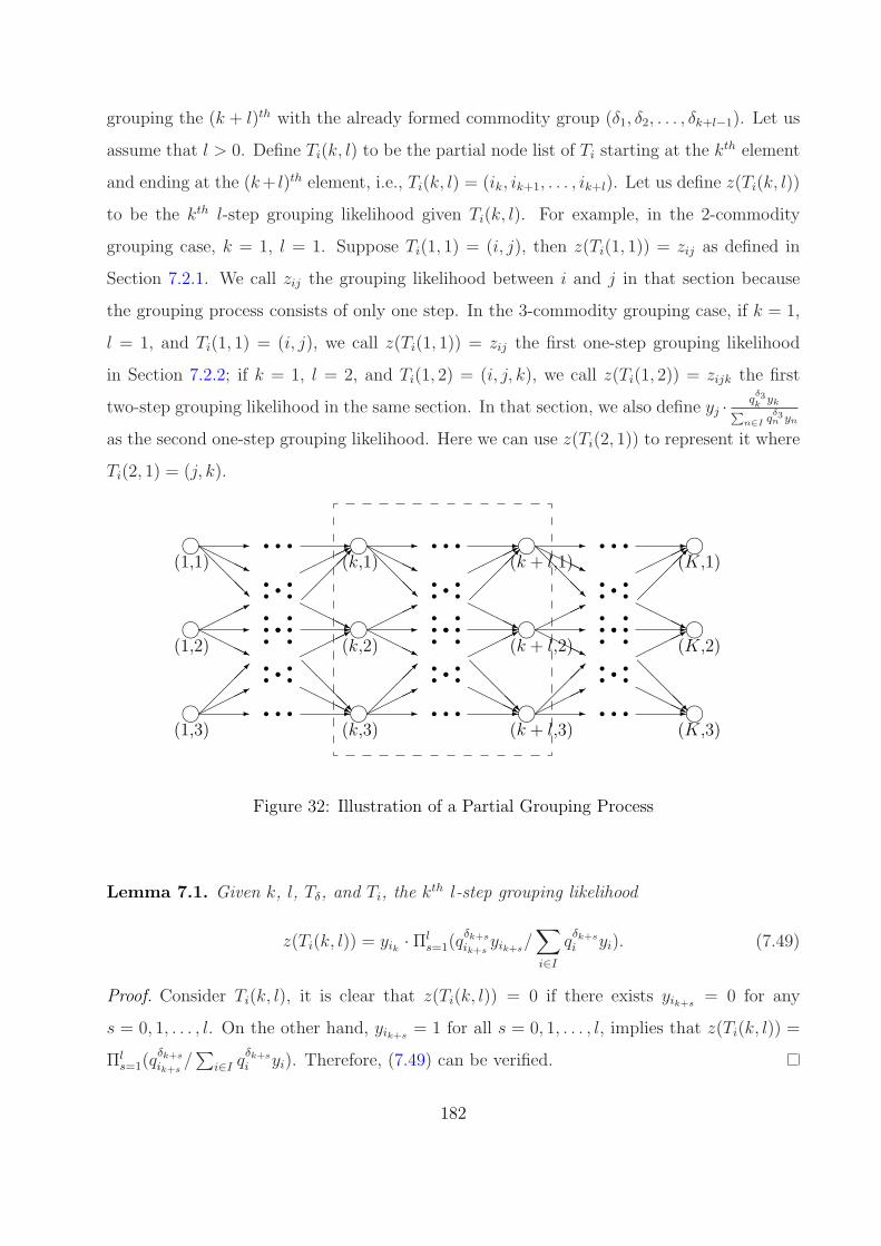
grouping the (k + l)th with the already formed commodity group (δ1, δ2, . . . , δk+l−1). Let us
assume that l > 0. Define Ti(k, l) to be the partial node list of Ti starting at the kth element
and ending at the (k+ l)th element, i.e., Ti(k, l) = (ik, ik+1, . . . , ik+l). Let us define z(Ti(k, l))
to be the kth l-step grouping likelihood given Ti(k, l). For example, in the 2-commodity
grouping case, k = 1, l = 1. Suppose Ti(1, 1) = (i, j), then z(Ti(1, 1)) = zij as defined in
Section 7.2.1. We call zij the grouping likelihood between i and j in that section because
the grouping process consists of only one step. In the 3-commodity grouping case, if k = 1,
l = 1, and Ti(1, 1) = (i, j), we call z(Ti(1, 1)) = zij the first one-step grouping likelihood
in Section 7.2.2; if k = 1, l = 2, and Ti(1, 2) = (i, j, k), we call z(Ti(1, 2)) = zijk the first
two-step grouping likelihood in the same section. In that section, we also define yj ·q
δ3k
ykP
n∈I qδ3n yn
as the second one-step grouping likelihood. Here we can use z(Ti(2, 1)) to represent it where
Ti(2, 1) = (j, k).
j
j
j
j
j
j
j
j
j
j
j
j
-
-
-
-
-
-
-
-
-
-
-
-
-
-
-
-
-
-
����*
����*
����*
����*
����*
����*
����*
����*
����*
����*
����*
����*
HHHHj
HHHHj
HHHHj
HHHHj
HHHHj
HHHHj
HHHHj
HHHHj
HHHHj
HHHHj
HHHHj
HHHHj
��
���
��
���
��
���
��
���
��
���
��
���@
@@@R
@@
@@R
@@
@@R
@@
@@R
@@
@@R
@@
@@Rr r r
r r r
r r r
r r r
r r r
r r r
r r r
r r r
r r r
r r r
r r r
r r r
r r r
r r r
r r r
r r r
r r r
r r r
r r r
r r r
r r r
rr
r
rr
r
rr
rrr
r
rr
r
rr
r
(1,1)
(1,2)
(1,3)
(k,1)
(k,2)
(k,3)
(k + l,1)
(k + l,2)
(k + l,3)
(K,1)
(K,2)
(K,3)
Figure 32: Illustration of a Partial Grouping Process
Lemma 7.1. Given k, l, Tδ, and Ti, the kth l-step grouping likelihood
z(Ti(k, l)) = yik · Πls=1(q
δk+s
ik+syik+s
/∑
i∈I
qδk+s
i yi). (7.49)
Proof. Consider Ti(k, l), it is clear that z(Ti(k, l)) = 0 if there exists yik+s= 0 for any
s = 0, 1, . . . , l. On the other hand, yik+s= 1 for all s = 0, 1, . . . , l, implies that z(Ti(k, l)) =
Πls=1(q
δk+s
ik+s/∑
i∈I qδk+s
i yi). Therefore, (7.49) can be verified.
182

Next we will study the relationship among grouping likelihoods with respect to different
segments of the grouping process with a given node list. For ease of exposition, we provide
the following definitions.
Definition 7.1. Suppose there are two lists T1 = (t1,1, t1,2, . . . , t1,K1) and T2 = (t2,1, t2,2, . . . , t2,K2)
with t1,K1 = t2,1. Operation “⊕” between two lists is defined as T1⊕T2 = (t1,1, t1,2, . . . , t1,K1 , t2,2,
. . . , t2,K2).
Definition 7.2. Suppose there are lists T1, T2, . . . , TS such that any two adjacent lists satisfy
the condition in Definition 7.1. Operation “∑
” among these lists is defined as∑S
i=1 Ti =
T1 ⊕ T2 ⊕ · · · ⊕ TS.
Operation “⊕” essentially links two lists with a specified order and requires that the last
element of the first list is identical to the first element of the second list. Thus, this operation
is not commutative. Operation “∑
” can be viewed as a shorthand notation of operation
“⊕” among several lists.
Lemma 7.2. Given a node list Ti = (i1, i2, . . . , iK). Suppose it can be partitioned such that
Ti =∑S
s=1 T si , then z(Ti) = ΠS
s=1z(T si ). Note that for any s = 1, . . . , S− 1, partial node lists
T si and T s+1
i overlap by one element, i.e., if the last element of T si is i, then the first element
of T s+1i is also i.
Proof. Suppose T si = (is0, . . . , i
sls) and the corresponding partial list of Tδ is T s
δ = (δs0, . . . , δ
sls)
for s = 1, . . . , S. Then z(T si ) is the (is0)
th ls-step grouping likelihood. By Lemma 7.1,
z(T si ) = yis0
· Πlst=1(q
δst
istyist
/∑
i∈I qδst
i yi). Then
ΠSs=1z(T s
i ) = yi10·Πl1
t=1
qδ1t
i1tyi1t
∑
i∈I qδ1t
i yi
·yi20·Πl2
t=1
qδ2t
i2tyi2t
∑
i∈I qδ2t
i yi
· · · · ·yiS0·ΠlS
t=1
qδSt
iStyiSt
∑
i∈I qδSt
i yi
.
For s = 1, . . . , S − 1, isls = is+10 implies that yis
lsyis+1
0= yis
ls. Hence,
ΠSs=1z(T s
i ) = yi10·Πl1
t=1
qδ1t
i1tyi1t
∑
i∈I qδ1t
i yi
·Πl2t=1
qδ2t
i2tyi2t
∑
i∈I qδ2t
i yi
· · · · ·ΠlSt=1
qδSt
iStyiSt
∑
i∈I qδSt
i yi
= z(Ti).
The second equality follows from Lemma 7.1.
183
Remark 7.1. In the 3-commodity grouping case, given Ti = (i, j, k), we have specified three
grouping likelihoods: the first one-step grouping likelihood zij; the second one-step grouping
likelihood zjk; and the first two-step grouping likelihood zijk. Note that there is only one two-
step grouping likelihood in a 3-commodity grouping process. It is clear that Ti = (i, j)⊕ (j, k)
and zijk = zijzjk.
So far we have considered a segment of the grouping process and defined the partial
grouping likelihood. For any segment of the grouping process, a partial node list is con-
structed. For example, Ti(k, l) = (ik, ik+1, . . . , ik+l) is a partial node list. Now let us consider
the set that contains all nodes in a partial node list. We define I(k, l) to be the set contain-
ing all nodes in Ti(k, l). Note that |I(k, l)| ≤ l + 1 since the same node may be selected at
different grouping steps.
For each k, 1 ≤ k ≤ K, let us rank {qδk
i }, ∀i ∈ I, in ascending and descending orders.
We construct the ascending and descending sequences, and denote {λδk
i } and {υδk
i }, ∀i ∈ I,
to be the corresponding index sequences, respectively. Define Λδks (D) and Υδk
s (D) to be the
first s elements of D ⊆ I in the respective sequences.
Proposition 7.1. Denote S ⊆ I to be the node set corresponding to the selected region.Given a partial node list Ti(k, l) and I(k, l), the set containing all nodes in Ti(k, l). IfI(k, l) ⊆ S, then
Πlt=1
qδk+t
ik+t
∑
i∈I(k,l) qδk+t
i +∑
i∈Υδk+ts (I\I(k,l))
qδk+t
i
≤ z(Ti(k, l)) ≤ Πlt=1
qδk+t
ik+t
∑
i∈I(k,l) qδk+t
i +∑
i∈Λδk+ts (I\I(k,l))
qδk+t
i
,
where s = |S| − |I(k, l)|.
Proof. Let us assume that S = I(k, l) ∪ {k1, k2, . . . , ks}. Then by Lemma 7.1,
z(Ti(k, l)) = Πlt=1
(
qδk+t
ik+t
∑
i∈I(k,l) qδk+t
i +∑
i∈S\I(k,l) qδk+t
i
)
.
By definition, we have
∑
i∈Λδk+ts (I\I(k,l))
qδk+t
i ≤∑
i∈S\I(k,l)
qδk+t
i ≤∑
i∈Υδk+ts (I\I(k,l))
qδk+t
i ,
for t = 1, . . . , l. Hence, the result follows.
184

Remark 7.2. In the 2-commodity grouping case, we know that k = 1, l = 1. Suppose
I(k, l) = {i, j} ⊆ S, where S is the node set corresponding to the selected region. Let
s = |S| − 2 and thus the grouping likelihood between i and j, zij, can be bounded as:
qδ2j
qδ2i + qδ2
j +∑
k∈Υδ2s (S\{i,j}) qδ2
k
≤ zij ≤qδ2j
qδ2i + qδ2
j +∑
k∈Λδ2s (S\{i,j}) qδ2
k
, if i 6= j, and
qδ2i
qδ2i +
∑
k∈Υδ2s+1(S\{i}) qδ2
k
≤ zij ≤qδ2i
qδ2i +
∑
k∈Λδ2s+1(S\{i}) qδ2
k
, if i = j.
This result is reduced to Theorem 6.2 and Corollary 6.4 in Chapter 6.2.1 when commodity
δ1 is organ, commodity δ2 is patient. Given a donor OPO id, qδ2i is the pure distribution
likelihood if i 6= id and the national-level flow likelihood if i = id. In Corollary 6.4 of Chapter
6.2.1, we use z0i instead of zii for each i ∈ I.
Proposition 7.2. Given k and l, let GRPP≥(s) be GRPP with imposition of the following
additional constraint:∑
i∈I yi ≥ s for s = |I(k, l)|, . . . , |I|. Then the following inequality is
valid for GRPP≥(s):
z(Ti(k, l)) ≤ yik · Πlt=1
qδk+t
ik+tyik+t
∑
i∈I(k,l) qδk+t
i +∑
i∈Λδk+ts−|I(k,l)|
(I\I(k,l))q
δk+t
i
. (7.50)
Proof. It is easy to see the result in the case where there exists a t = 0, 1, . . . , l such thatyik+t
= 0. If yik+t= 1 for all t = 0, 1, . . . , l, the result follows directly from Proposition 7.1
as s− |I(k, l)| =∑
i∈I yi − |I(k, l)| = |S| − |I(k, l)|. If∑
i∈I yi = s′ > s, we have
z(Ti(k, l)) ≤ Πlt=1
0
B
B
@
qδk+t
ik+t
P
i∈I(k,l) qδk+t
i +P
i∈Λδk+t
s′−|I(k,l)|(I\I(k,l))
qδk+t
i
1
C
C
A
≤ yik·Πl
t=1
0
B
B
@
qδk+t
ik+tyik+t
P
i∈I(k,l) qδk+t
i +P
i∈Λδk+t
s−|I(k,l)|(I\I(k,l))
qδk+t
i
1
C
C
A
.
The first inequality is due to Proposition 7.1. The second inequality holds for s′ > s and
yik+t= 1, t = 0, . . . , l.
Proposition 7.3. Given k and l, let GRPP≤(s) be GRPP with imposition of the following
additional constraint:∑
i∈I yi ≤ s for s = |I(k, l)|, . . . , |I|. Then the following inequality is
valid for GRPP≤(s):
yik · Πlt=1
qδk+t
ik+tyik+t
∑
i∈I(k,l) qδk+t
i +∑
i∈Υδk+ts−|I(k,l)|
(I\I(k,l))q
δk+t
i
≤ z(Ti(k, l)). (7.51)
185

Proof. It is easy to see the result in the case where there exists a t = 0, 1, . . . , l such thatyik+t
= 0. If yik+t= 1 for all t = 0, 1, . . . , l, the result follows directly from Proposition 7.1
as s− |I(k, l)| =∑
i∈I yi − |I(k, l)| = |S| − |I(k, l)|. If∑
i∈I yi = s′ < s, we have
z(Ti(k, l)) ≥ Πlt=1
0
B
B
@
qδk+t
ik+t
P
i∈I(k,l) qδk+t
i +P
i∈Υδk+t
s′−|I(k,l)|(I\I(k,l))
qδk+t
i
1
C
C
A
≥ yik·Πl
t=1
0
B
B
@
qδk+t
ik+tyik+t
P
i∈I(k,l) qδk+t
i +P
i∈Υδk+t
s−|I(k,l)|(I\I(k,l))
qδk+t
i
1
C
C
A
.
The first inequality is due to Proposition 7.1. The second inequality holds for s′ < s and
yik+l= 1, t = 0, . . . , l.
Theorem 7.1. Given k and l, let GRPP=(s) be GRPP with imposition of the followingadditional constraint:
∑
i∈I yi = s for s = |I(k, l)|, . . . , |I|. Then the following inequality isvalid for GRPP=(s):
yik·Πl
t=1
0
B
B
@
qδk+t
ik+tyik+t
P
i∈I(k,l) qδk+t
i +P
i∈Υδk+t
s−|I(k,l)|(I\I(k,l))
qδk+t
i
1
C
C
A
≤ z(Ti(k, l)) ≤ yik·Πl
t=1
0
B
B
@
qδk+t
ik+tyik+t
P
i∈I(k,l) qδk+t
i +P
i∈Λδk+t
s−|I(k,l)|(I\I(k,l))
qδk+t
i
1
C
C
A
.
(7.52)
Proof. It is easy to see the result in the case where there exists a t = 0, 1, . . . , l such that
yik+t= 0. If yik+t
= 1 for all t = 0, 1, . . . , l, the result follows directly from Proposition
7.1.
Corollary 7.1. For any Ti(k, l), the following bounding constraint is valid for the generalized
pricing problem GRPP:
yik · Πlt=1
(
qδk+t
ik+tyik+t
∑
i∈I qδk+t
i
)
≤ z(Ti(k, l)) ≤ yik · Πlt=1
(
qδk+t
ik+tyik+t
∑
i∈I(k,l) qδk+t
i
)
.
Proof. The upper bound follows from Proposition 7.2 as s = |I(k, l)| and the lower bound
follows from Proposition 7.3 as s = |I|.
Corollary 7.2. Define T ′i (k, l) to be any permutation of Ti(k, l). The same bounding in-
equality (7.52) for Ti(k, l) also holds for z(T ′i (k, l)).
Remark 7.3. In the 2-commodity grouping case, Propositions 7.2 and 7.3, and Corollary
7.1 are reduced to Propositions 6.4 and 6.5, and Corollary 6.3 in Section 6.2, respectively,
when each u(i1,i2) is restricted as a binary variable, i.e., u(i1,i2) = yi1yi2 ,∀i1, i2 ∈ I.
186

Remark 7.4. The generalization of Corollaries 6.4 and 6.5 in Section 6.2 is included in
the results presented in Theorem 7.1 and Corollary 7.1 as those for Ti(1, 1) = (i1, i2) where
i1 = i2. Note that yi1yi2 = yi1 = yi2 in that case.
Remark 7.5. Given k and l, let us denote P=s to be the feasible solution region of GRPP=(s)
for s = |I(k, l)|, . . . , |I|. When s = |I|, z(Ti(k, l)) = Πlt=1(q
δk+t
ik+t/∑
i∈I qδk+t
i ), and P=s becomes
one point (all z variables are uniquely determined). This corresponds to the case where all
y variables have been fixed to 1.
Remark 7.6. Let us denote P≥s and P≤
s to be the feasible solution regions of GRPP≥(s) and
GRPP≤(s), respectively. It is clear that P≥s+1 ⊆ P≥
s and P≤s ⊆ P≤
s+1, ∀s = 0, 1, . . . , |I| − 1.
187
8.0 SUMMARY AND FUTURE RESEARCH
8.1 SUMMARY
This dissertation addresses the issue of facilitating organ sharing in the U.S. organ transplan-
tation and allocation network. It focuses on the aspect of organizing geographic transplan-
tation and allocation service areas in the hierarchical allocation system. To the best of our
knowledge, our work is the first considering this problem. The majority of previous research
has taken the individual patient’s perspective and attempted to answer the question whether
an ESLD patient should accept or reject an organ offer. Much of the previous work that
sought global allocation strategies proposed a complete redesign of the allocation policy only
at the local level. Unlike these previous efforts, we optimize the entire hierarchical system
with the existing allocation policy. This means that the political barriers to implementing
the results of our research are reduced. Furthermore, it could create potential impact on the
entire allocation network.
This dissertation is intended to develop a modeling framework to assist policy makers in
refining the geographic composition of the hierarchical network to facilitate organ sharing.
The framework we develop is a set-partitioning framework in which we estimate a certain
allocation efficiency related outcome, which is associated with each potential region, and
select the best set of potential regions such that the total welfare of the entire system is
maximized. To estimate the outcome, we take a macro-level viewpoint and introduce the
notion of proportional allocation. Chapters 4 and 5 consider two estimates for the intra-
regional donor-recipient pairing likelihood: the estimate based on patient population, in
which we assume the pairing likelihood is proportional to the patient population of the
donor OPO; and the single national list based estimate, in which we assume the pairing
188

likelihood is proportional to the probability that organs are distributed in the network when
all patients are awaiting transplants on one single national waiting list. The latter estimate
is more accurate than the former one in that (1) it incorporates patient heterogeneity in
terms of clinical and demographic characteristics; (2) it considers the effect of national-level
allocation.
In Chapter 3, an extension from the set-partitioning formulation addresses both alloca-
tion efficiency and geographic equity. The resulting model is a two-objective combinatorial
optimization model with an additional decision variable measuring equity and a class of
constraints restricting the considered equity measure.
In Chapter 4, to use the single national list based estimate, we need to estimate a few
parameters in the situation that all patients are on the same national waiting list. However,
this situation does not exist in reality because of the current three-tier hierarchical structure
of the network. To estimate parameters that are meaningful in such a situation, we adapt a
clinically based organ transplantation and allocation simulation model in Chapter 4. Using
the same simulation model, we also compare the geographic partition obtained from our set-
partitioning model with the current regional configuration to verify the benefit of optimal
region design. In Chapter 4, we also present a model that addresses the effect of national-level
allocation by borrowing the spill-and-recapture technique from the airline fleet assignment
problem.
With either estimate, we solve the region design problem through explicit enumeration
of regions. Since it is computationally prohibitive to solve instances with all possible regions
constructed based on the 59 OPOs, we reduce the solution space by only consider contiguous
regions with no more than 8 OPOs. We report the improvement on allocation efficiency
by using this approach in Chapters 3 and 4. This improvement is also verified through
simulation.
Given the computational challenge presented in Chapters 3 and 4, we apply branch and
price in Chapter 5 to solve the optimal region design problem. We adaptively generate
“promising” regions at each node of the branch-and-bound search tree. We derive a mixed-
189

integer programming pricing problem that is proved to be NP-hard. Compared to results
reported in Chapter 4, further improvement is obtained within a reasonable amount of time.
This demonstrates the applicability of our branch-and-price solution.
Knowing that solving the pricing problem is the most computationally intensive compo-
nent of the solution, we explore various ideas to alleviate this computational burden. One
main idea is geographic decomposition that attempts to solve many smaller-scale pricing
problems instead of a big problem. Various computational issues are discussed to select the
best solution. The other main idea, presented in Chapter 6, is to study the pricing problem
more closely, which includes analyzing alternative formulations of the pricing problem and
deriving strong valid inequalities for the pricing problem.
In Chapter 7, we generalize the notion of proportional allocation. Consequently, we
generalize the column generation approach and a class of valid inequalities.
8.2 FUTURE RESEARCH
This research consists of two parts, the modeling part and the solution part. Therefore, two
directions of future research are model refinement and extension, and solution improvement.
Section 8.2.1 presents several ideas to refine and extend the model. Section 8.2.2 discusses
a few approaches to improve the branch-and-price solution. We will also discuss a few
generalization ideas in Section 8.2.3.
8.2.1 Model Refinement and Extension
Combining various modeling perspectives. This work takes a societal perspective to
answer the question whether the current geographic organization is optimal. To model the
complex allocation system in a more sophisticated way, we need to consider the patient’s
perspective and integrate the two perspectives. The following are three potential directions
for the integration. First in the current model, we treat patient autonomy, i.e., patient’s
right to accept/reject an organ offer, in a relatively crude way by assuming identical accep-
190

tance/rejection probability among patients. Therefore, one direction of future work is to
refine the current model to capture patient preferences. Our objective is still to maximize
the social welfare of the entire system. Second, addressing the social welfare of the system
and each individual’s benefit simultaneously may be necessary. This may lead to a multi-
objective optimization problem, which is an extension of the current modeling framework
with incorporation of objectives measuring individual benefit. It is clear that there is a
conflict among patients in terms of their benefits. Third, due to patient autonomy, a patient
would evaluate her decision based on the information she is able to access regarding her
position on the waiting list as well as the composition of the waiting list. Hence, there is a
question of to what extent she should be allowed to access the information. The goal along
this direction is to understand the impact of information accessibility and, as a result, to
develop a better allocation policy to facilitate organ sharing.
Modeling system dynamics and uncertainty. In our current model, we take a macro-
level viewpoint to estimate the specified outcome associated with either allocation efficiency
or equity. Essentially, we study the group behavior of patients and organs. Given the
highly dynamic and stochastic nature of the allocation system, incorporating dynamics and
stochasticity is necessary in future work. First of all, organ procurement and patient listing
occur dynamically. Clinical and demographic characteristics of procured organs and listed
patients are uncertain in nature. Second, when an OPO matches patients with organs or
a patient accepts/rejects an organ offer, the decision is made based on the ever-changing
composition of the waiting list, and clinical and demographic characteristics of organs and
patients. Finally, for each decision that an OPO or a patient makes, risk is involved. Our
objective in the future is to build a robust and reliable allocation decision model.
Addressing both efficiency and equity. Although this work largely focuses on allocation
efficiency, we make an attempt to address allocation equity as well. In fact, efficiency and
equity are considered in almost every social welfare system. In each outcome category, there
are many associated attributes. For each attribute, there may also be many associated
subattributes. For efficiency, we may consider transplant quantity, transplant survival rate,
191

or transplant waiting time as attributes. For each efficiency attribute, subattributes are
specified at various time points. For example, for the attribute transplant survival rate,
subattributes could be 1-year survival rate, 3-year survival rate, and 5-year survival rate. For
equity, we may consider geographic equity, racial/ethnic equity, socioeconomic equity, etc.
For each equity attribute, subattributes are specified among various stratified subgroups. For
example, for the attribute racial/ethnic equity, subattributes could be the identical system
outcomes associates with African-Americans and Hispanics. As a result, we need to make
decisions with respect to multiple criteria. Multi-objective optimization, or in a broader
sense, multicriteria decision making will be considered.
Modeling the entire hierarchy. In our current model, we only estimate allocation ef-
ficiency at the regional level. To capture the impact of the three-tier transplantation and
allocation system, we need to estimate allocation efficiency at all three levels. This means
that we need to estimate potential allocation efficiency accumulated at various steps in the
allocation algorithm as a transplantable organ proceeds through the allocation process. The
most critical part in modeling allocation efficiency throughout the entire hierarchy is model-
ing the allocation at the national level. In this work, we present an estimate for the effect of
national-level allocation on regional-level allocation. However, the estimate does not allow
network interdependency. In our case, it means that national-level allocation in one region is
not dependent upon the composition of other regions. Barnhart et al. [23] described a new
modeling and algorithmic approach for fleeting assignment that models spill and recapture
as a function of assigned capacity across an entire airline network and not just a single flight
leg. Similarly, we may develop a new model for our problem that models spill and recapture
as a function of all OPOs in the network and not just a single OPO.
Integrating simulation and optimization. In our current model, we use the intra-
regional transplant cardinality to measure allocation efficiency analytically. This estimate
is, at best, a good proxy. The main reason we use this estimate is that almost all medically
realistic outcomes are hard to express analytically. One possible research topic is to integrate
simulation into the column generation framework. The simulation model will give us a more
192

faithful representation of the real-world system. Once a column is generated, we input it
to the simulation model to estimate the system outcome associated with it. However, it is
time-consuming to even estimate the outcome for one potential region. Therefore, this future
research direction will primarily focus on how to obtain useful information and evaluate the
pricing problem with simulation. Another possible research topic is to develop simulation-
based metaheuristic methods.
Extension to other types of organs. In this work, we use liver transplantation and
allocation as an example of the region design problem. The modeling framework we build
and techniques we apply in this research can be used to address the transplantation and
allocation of other types of organs that raises similar issues. For example, heart disease has
been consistently ranked the No. 1 cause of death in the United States [86], accounting
for nearly 700,000 deaths in 2002 alone. Many patients with heart diseases require heart
transplants. A future research topic will be how to organize OPO service areas for heart
transplantation and allocation. Furthermore, it is conceivable that the best set of OPOs
would vary among different types of organs. An interesting research question is what is the
best set of OPOs considering all types of organs.
8.2.2 Branch-and-Price Solution Improvement
To solve our optimal region design problem using an exact algorithm, we show the need for
branch and price, which embeds column generation within a branch-and-bound framework.
There are many important computational issues that need to be considered in our problem.
Some of them are commonly encountered in all branch-and-price applications. Some others
are unique in our problem.
Initial Solution. To start the column generation scheme, an initial restricted master prob-
lem has to be provided. In our case, it is easy to provide an initial restricted master. However,
it is not obvious which one is good. In this work, we compare a few initial restricted master
problems. There is a need for more computational investigation.
193
Column Management. In a maximization linear program, any column with positive re-
duced cost is a candidate to enter the basis. Therefore, we do not always have to solve
the pricing problem to optimality to find a column with the highest reduced cost. In this
work, knowing the pricing problem is computationally intensive, we apply geographic de-
composition, which is an approximation algorithm in a loose sense. As long as it produces
a column with positive reduced cost, that column will be added to the restricted master. It
has been observed that designing region covers is critical. Consequently, we want to predict
the impact of each region cover on the construction of the optimal solution a priori and
redesign region covers dynamically throughout the solution procedure. This may require us
to understand the dual solution better at each iteration. With geographic decomposition,
we may generate more than one column with positive reduced cost. For each region cover,
we also test a number of column generation strategies in terms of the number of columns
to be generated at each iteration. Generating fewer columns will reduce the computation
time per iteration. However, the number of iterations may increase. In addition, we do not
continue to prove optimality of the entire restricted master after geographic decomposition
fails to produce a column with positive reduced cost. Such a scheme results in a trade-off
between the solution quality and solution time.
To summarize, we will study the selection of a subset of “good” regions. The following
is some previous work from which we may obtain some insights. Vanderbeck [212] discussed
many relevant issues and suggested that using approximation algorithms and adding multiple
columns works best when the pricing problem is computationally intensive. Savelsbergh and
Sol [184] described a fast heuristic approach for generating columns with positive reduced
costs. They took existing columns with reduced cost equal to zero and employed fast local
improvement algorithms to construct columns with a positive reduced cost. To draw a
more decisive conclusion on the best algorithmic choice for our problem, a more thorough
computational investigation is required.
The tailing-off effect. We have observed the tailing-off effect that many column gener-
ation schemes exhibit, i.e., requiring a large number of iterations to prove LP optimality.
194
Clearly, there is a trade-off between the computational effort associated with computing
strong bounds and evaluating small trees and computing weaker bounds and evaluating big-
ger trees. Naturally, one future research topic will be to explore this trade-off, especially
considering our pricing problem is hard to solve. Instead of solving the linear program to
optimality, i.e., we can choose to prematurely terminate the column generation process and
work with bounds on the final LP value. The following is some previous work from which
we may gain some insights. Farley [84], Lasdon [134], and Vanderbeck and Wolsey [214]
described simple and relatively easy-to-compute bounds on the final LP value based on the
LP value of the current restricted master problem and the current reduced costs.
Pricing Integer Programs. Given the fact that our pricing problem is hard to solve theo-
retically and practically, we also need to improve the pricing problem solution fundamentally
beyond algorithmic improvements in column generation. One possible future research is to
study computational performance of the two classes of valid inequalities derived in Chapter
6.
Other possible improvement directions. First, we may want to study alternative dual
solutions associated with the restricted master problem. Second, we may want to study
primal heuristics to find a good integer feasible solution when proving optimality is of lesser
or no importance. Moreover, an effective heuristic algorithm may help the branch-and-price
solution. Third, we may want to combine column and row generations especially when we
consider applying branch and price to the second model presented in Chapter 3 addressing
both efficiency and equity.
8.2.3 Generalization
Chapter 7 generalizes the proportional allocation scheme in terms of the number of group-
ing commodities in a network. Three other possible generalizations are included as follows.
When considering how to allocate commodities from one node to various nodes in a network,
proportional allocation is one of many schemes. It assumes that items of a commodity are
195

allocated proportionally based on some quantity associated with each node. An alternative
allocation scheme is to allocate items of a commodity such that the accrued benefit is max-
imized. This means that we solve a transportation problem once the allocation region is
known. For each region, there is an embedded transportation problem. The second possible
direction of generalization is on hierarchical allocation with an arbitrary number of levels in
the hierarchy. We may consider commodity flow throughout the hierarchy. In the current
model, we only consider the flow from Phase 4 to Phase 5 of the allocation process. The last
possible direction of generalization is to consider multiple types of commodities instead of
one. In our case, we may want to consider multiple types of organs or patients with different
diseases. Presumably, the allocation of multicommodities between nodes is restricted due
to arc capacity. We believe that all these possible directions of generalization will pave the
way for a better understanding of issues arising in the organ transplantation and allocation
network.
196

APPENDIX A
APPLICATIONS OF INTEGER PROGRAMMING COLUMN
GENERATION
197

Table 30: Applications of Integer Programming Column Generation
Applications References
vehicle routing problems [4, 66, 67, 140, 141, 175]
crew scheduling problems [31, 66, 68]
multiple traveling salesman problem with time windows [72]
real-time dispatching of automobile service units [127]
multiple pickup and delivery problem with time windows [143, 193]
airline crew pairing [11, 49]
air network design for express shipment service [24]
airline scheduling generation [82]
fleet assignment and aircraft routing and scheduling [18, 65, 114]
job grouping for flexible manufacturing systems [50]
grouping and packaging of electronic circuits [78]
bandwidth packing in telecommunication networks [160]
traffic assignment in satellite communication systems [174]
course registration at a business school [182]
graph partitioning in VLSI and compiler design [212]
graph partitioning in political redistricting [150]
single-machine multi-item lot-sizing [212]
bin packing and cutting stock problems [205, 206, 207, 209, 210, 213]
integer multicommudity flows [20, 21]
maximum stable set problem [33]
probabilistic maximum satisfiability problem [105]
minimum cut clustering [119]
graph coloring [151]
generalized assignment problem [183]
198

APPENDIX B
A LIST OF ORGAN PROCUREMENT ORGANIZATIONS
199

Table 31: A List of Organ Procurement Organizations [88]
Label Name Location∗ RegionALOB Alabama Organ Center Birmingham, AL 3AROR Arkansas Regional Organ Recovery Agency Little Rock, AR 3AZOB Donor Network of Arizona Phoenix, AZ 5CADN California Transplant Donor Network Oakland, CA 5CAGS Golden State Donor Services Sacramento, CA 5CAOP OneLegacy Los Angeles, CA 5CASD Lifesharing Community Organ & Tissue Donation San Diego, CA 5CORS Donor Alliance Denver, CO 8CTOP LifeChoice Donor Services Windsor, CT 5DCTC Washington Regional Transplant Consortium Falls Church, VA 2FLFH TransLife Orlando, FL 3FLMP Life Alliance Organ Recovery Agency Miami, FL 3FLSW LifeLink of Southwest Florida Fort Myers, FL 3FLUF LifeQuest Organ Recovery Services Gainesville, FL 3FLWC LifeLink of Florida Tampa, FL 3GALL LifeLink of Georgia Atlanta, GA 3HIOP Organ Donor Center of Hawaii Honolulu, HI 6IAOP Iowa Donor Network Iowa City, IA 8ILIP Gift of Hope Organ & Tissue Donor Network Elmhurst, IL 7INOP Indiana Organ Procurement Organization Indianapolis, IN 10KYDA Kentucky Organ Donor Affiliates Louisville, KY 11LAOP Louisiana Organ Procurement Agency Metairie, LA 3MAOB New England Organ Bank Newton, MA 1MDPC Transplant Resource Center of Maryland Baltimore, MD 2MIOP Gift of Life Michigan Ann Arbor, MI 10MNOP LifeSource Upper Midwest Organ Procurement Organization St. Paul, MN 7MOMA Mid-America Transplant Services St Louis, MO 8MSOP Mississippi Organ Recovery Agency Jackson, MS 3MWOB Midwest Transplant Network Westwood, KS 8NCCM Lifeshare of the Carolinas Charlotte, NC 11NCNC Carolina Donor Services Greenville, NC 11NEOR Nebraska Organ Recovery System Omaha, NE 8NJTO New Jersey Organ and Tissue Sharing Network OPO Springfield, NJ 2NMOP New Mexico Donor Services Albuquerque, NM 5*: The location of each OPO is as in July 2003. There have been a few changes lately.
200

Table 32: A List of Organ Procurement Organizations (Contd.)
Label Name Location∗ RegionNVLV Nevada Donor Network Las Vegas, NV 5NYAP Center for Donation and Transplant Albany, NY 9NYFL Finger Lakes Donor Recovery Program Rochester, NY 9NYRT New York Organ Donor Network New York, NY 9NYWN Upstate New York Transplant Services Inc Buffalo, NY 9OHLB LifeBanc Cleveland, OH 10OHLC Life Connection of Ohio Dayton, OH 10OHLP Lifeline of Ohio Columbus, OH 10OHOV LifeCenter Organ Donor Network Cincinnati, OH 10OKOP LifeShare Transplant Donor Services of Oklahoma Oklahoma City, OK 4ORUO Pacific Northwest Transplant Bank Portland, OR 6PADV Gift of Life Donor Program Philadelphia, PA 2PATF Center for Organ Recovery and Education Pittsburgh, PA 2PRLL LifeLink of Puerto Rico Guaynabo, PR 3SCOP LifePoint Charleston, SC 11TNDS Tennessee Donor Services Nashville, TN 11TNMS Mid-South Transplant Foundation Memphis, TN 11TXGC LifeGift Organ Donation Center Houston, TX 4TXSA Texas Organ Sharing Alliance San Antonio, TX 4TXSB Southwest Transplant Alliance Dallas, TX 4UTOP Intermountain Donor Services Salt Lake City, UT 5VATB LifeNet Virginia Beach, VA 11WALC LifeCenter Northwest Donor Network Bellevue, WA 6WISE Wisconsin Donor Network Milwaukee, WI 7WIUW Organ Procurement Organization at the University of Wisconsin Madison, WI 7*: The location of each OPO is as in July 2003. There have been a few changes lately.
201
APPENDIX C
DETAILED DESCRIPTION OF THE BCP IMPLEMENTATION
This appendix describes the detailed implementation of our branch-and-price application
using BCP. Since our implementation adapts the one for the axial assignment problem (AAP)
in Galati [93], we do not repeat the description that appears in that paper. we call the region
design problem RSP in this appendix for ease of exposition.
In order to implement a branch-and-price algorithm using BCP, there are a minimal set
of functions that must be written by the user. In this section we will describe each of these
functions as they have been used in applying branch and price to solve the region design
problem. The application source code is divided into the following directories:
• LP: functions used by the linear programming process,
• TM: functions used by the tree manager process,
• Member: functions used to input instances,
• Data: most of the data used to define instances,
• Run: a run directory including parameter files.
Data Structure
• Member/RSP.cpp
The RSP class simply defines a storage container for an instance of RSP. This includes the
organ data oi, the pure distribution likelihood lij, and the pure national flow likelihood
l0i , and the cold ischemia time, denoted as tij.
202
• include/RSP user data.hpp
The RSP user data class, derived from BCP user data, stores some additional infor-
mation related to branching. In our case, we have implemented two branching rules,
branching on variables and branching on OPO pairs.
• include/RSP var.hpp
The RSP var class, derived from BCP var algo, stores solution information including
the indices of OPOs contained in each region in the optimal configuration and the regional
benefit of each region.
Initialization
• Member/RSP init.cpp
In order to initialize the interface to BCP, we need to create an instance of each process
that will be used. In our case we need to initialize:
– BCP user init(): the user interface,
– lp init(): the LP process, and
– tm init(): the TM process.
In tm init(), in addition to initializing the TM process, we read in data files that
describe a RSP instance.
Parameters
• Parameters
In the Run directory, we specify a list of parameters used for our application in a param-
eter file. This list includes three types of parameters, BCP parameters, RSP parameters,
and solution parameters.
A description of the various BCP parameters used for the LP process and the TM
process is available in the Doxygen note on the COIN-OR website [87]. In the class of
RSP parameters, we specify the input files that describe the instance, the region covers
design, and the set of initial columns. Most of solution parameters are used to specify
all solution options discussed in Chapter 5.6.3. They are listed as follows:
203

– regionSP subprob use smallones indicates if we use geographic decomposition.
– regionSP subprob use callback indicates if we use CPLEX callback to add to the
restricted master problem not only the column that prices out the most favorably
but also other columns generated in the pricing problem solution process.
– regionSP subprob numCols perIter specifies the number of feasible columns added
to the restricted master problem.
– regionSP subprob epgap corresponds to the CPLEX MIP solution parameter
CPX PARAM EPGAP that specifies the relative mipgap tolerance in CPLEX.
– regionSP subprob heurfreq specifies the CPLEX MIP solution parameter
CPX PARAM HEURFREQ that specifies the MIP heuristic frequency in CPLEX.
– regionSP subprob mipemphasis specifies the CPLEX MIP solution parameter
CPX PARAM MIPEMPHASIS that specifies the MIP emphasis indicator in CPLEX.
In addition to the above solution parameters, Parameter regionSP subprob branch type
indicates which branching rule we use, branching on variables or branching on OPO pairs.
For more information on the CPLEX related solution parameters, we refer to the CPLEX
user’s manual [113].
• TM/RSP tm param.cpp specifies variables that corresponding to parameters used in the
TM module. It includes the specification of data files describing the RSP instance. This
file serve the purpose of linking the parameter file with other source codes in the TM
directory.
• LP/RSP lp param.cpp specifies variables that corresponding to parameters used in the
LP module. It includes the specification of all solution parameters. This file also serves
the purpose of linking the parameter file with other source codes in the LP directory.
Tree Manager
• TM/RSP tm.cpp::initialize core():
In this function, we describe which decision variables and which constraints are core. If
a decision variable or constraint is the core, it can never be removed from the restricted
master problem once the problem is created. We have no core decision variables. The
core constraints are all set-partitioning constraints.
204

• TM/RSP tm.cpp::create root():
In this function, we initialize the root node of the branch-and-price tree. To achieve this,
we can either load all single-OPO regions or read an initial set of columns from a file. For
the initial set of columns, we consider several column generation initialization schemes.
Linear Program
• LP/RSP lp.cpp::compute lower bound(): In this function, we implement the two op-
tions with respect to geographic decomposition. If we use geographic decomposition,
we call function readin divisions() to input the region covers design. In addition, if
we use geographic decomposition, we also call function generate vars multiple() or
generate vars single() to generate multiple columns with positive reduced costs or a
single column with the most positive reduced cost for each region cover. If we do not
use geographic decomposition, the two above functions generate multiple columns with
positive reduced costs or a single column with the most positive reduced cost for the
entire country. At the end of this function, if we cannot find any column(s) with positive
reduced cost, we terminate the execution.
• LP/RSP lp.cpp::generate vars in lp():
In this function, we look for column(s) with positive reduced cost and add such column(s)
to the restricted master. The identification of positive reduced cost has already been done
in computer lower bound().
• LP/RSP lp.cpp::generate vars multiple() and
LP/RSP lp.cpp::generate vars single():
In each of these two functions, we call function construct cost() and actually generate
columns that price out favorably.
• LP/RSP lp.cpp::construct cost():
In this function, we compute the objective coefficient (regional benefit) for each generated
column.
• LP/RSP lp.cpp::solve pricing problem multicols(),
LP/RSP lp.cpp::solve pricing problem singlecol mostrc(), and
LP/RSP lp.cpp::solve pricing problem rounding():
205
In each of these three functions, we construct the basic pricing problem and then add
constraints fixing variables and modeling relationships between variables in the solution
process. Each function has the option to construct the pricing problem based on the entire
country or a region cover. For the pricing problem solution, we specify several CPLEX
MIP solution parameters in the first two functions. For the pricing problem solution,
we also use CPLEX callback in the first two functions to specify the number of columns
generated at each iteration of column generation. We only solve the LP relaxation of the
pricing problem in the third function and apply two rounding heuristics.
• LP/RSP lp branch.cpp::select branching candidates():
This function creates candidate branching objects using branching on OPO pairs or
branching on variables.
• LP/RSP lp branch.cpp::set user data for children():
This function stores information about which pair of OPOs is selected or which variables
are fixed.
• LP/RSP lp branch.cpp::branch on OPOpair():
This function specifies the node pair selection rule. That is, choose a pair of OPOs s and
t such that∑
r∈Is∩Itxr is closest to 0.5.
• LP/RSP lp branch.cpp::appending branching pairs():
In this function, branching candidates are constructed as a BCP lp branching object
with a number of arguments. This function applies to both branching rules that are
considered.
There are several utility functions in the LP module, e.g., computing the objective coef-
ficient for a given column, computing the objective value for a given regional configuration,
and converting a cold ischemia time tij to an organ acceptance probability αij.
206

APPENDIX D
COLUMN GENERATION EFFECT
207

Table 33: Column Generation Effect (20 covers and each cover with 14 OPOs)
p0 = 0.9 p0 = 1.1
CPU Num Num Avg Cols Avg Cols CPU Num Num Avg Cols Avg Cols
Instance Strategy Time (s) Iters Cols per Iter per Cover Time (s) Iters Cols per Iter per Cover
1 9248 73 997 13.7 49.9 9082 68 994 14.6 49.7
2 5076 37 948 25.6 47.4 11940 58 1068 18.4 53.4
3 3977 31 1107 35.7 55.4 4453 32 1101 34.4 55.1
20 14 1 4 4284 29 1055 36.4 52.8 4009 27 1086 40.2 54.3
5 3191 24 1018 42.4 50.9 3632 24 1114 46.4 55.7
6 3602 24 1088 45.3 54.4 4004 25 1173 46.9 58.7
A 3357 23 1095 47.6 54.8 4859 25 1167 46.7 58.4
B 6435 36 541 15.0 27.1 6172 33 546 16.5 27.3
1 7503 77 1052 13.7 52.6 9708 85 1059 12.5 53.0
2 4346 41 1051 25.6 52.6 4234 40 1069 26.7 53.5
3 3928 34 1100 32.4 55.0 4082 31 1029 33.2 51.5
20 14 2 4 3522 28 1057 37.8 52.9 3568 27 1067 39.5 53.4
5 3395 26 1070 41.2 53.5 3998 27 1046 38.7 52.3
6 3318 24 1094 45.6 54.7 4159 26 1042 40.1 52.1
A 3528 24 1072 44.7 53.6 3909 24 1098 45.8 54.9
B 5768 37 578 15.6 28.9 6532 36 550 15.3 27.5
Table 34: Column Generation Effect (20 covers and each cover with 10 OPOs)
p0 = 0.9 p0 = 1.1
CPU Num Num Avg Cols Avg Cols CPU Num Num Avg Cols Avg Cols
Instance Strategy Time (s) Iters Cols per Iter per Cover Time (s) Iters Cols per Iter per Cover
1 471 52 653 12.6 32.7 906 52 587 11.3 29.4
2 317 31 640 20.6 32.0 229 25 574 23.0 28.7
3 221 23 640 27.8 32.0 235 23 689 30.0 34.5
20 10 1 4 187 20 603 30.2 30.2 235 21 652 31.1 32.6
5 186 20 663 33.2 33.2 202 20 663 33.2 33.2
6 167 18 628 34.9 31.4 199 19 629 33.1 34.6
A 209 20 660 33.0 33.0 205 19 653 34.4 32.7
B 346 30 437 14.6 21.9 262 24 382 15.9 19.1
1 294 43 596 13.9 29.8 329 43 591 13.7 29.6
2 235 28 647 23.1 32.4 243 27 632 23.4 31.6
3 167 21 644 30.7 32.2 173 20 613 30.7 30.7
20 10 2 4 190 22 653 29.7 32.7 172 20 669 33.5 33.5
5 159 19 676 35.6 33.8 202 21 665 31.7 33.3
6 189 21 649 30.9 32.5 205 21 683 32.5 34.2
A 123 16 622 38.9 31.1 157 18 592 32.9 29.6
B 206 24 398 16.6 19.9 266 26 410 15.8 20.5
208

Table 35: Column Generation Effect (20 covers and each cover with 8 OPOs)
p0 = 0.9 p0 = 1.1
CPU Num Num Avg Cols Avg Cols CPU Num Num Avg Cols Avg Cols
Instance Strategy Time (s) Iters Cols per Iter per Cover Time (s) Iters Cols per Iter per Cover
1 90.7 36 388 10.8 19.4 138 26 379 14.6 19.0
2 57.2 22 405 18.4 20.3 88.9 18 398 22.1 19.9
3 52.8 20 427 21.4 21.4 96.4 18 427 23.7 21.4
20 8 1 4 43.5 17 466 27.4 23.3 97.4 18 431 23.9 21.6
5 53.4 19 447 23.5 22.4 85.6 16 426 26.6 21.3
6 52.8 19 447 23.5 22.4 87.4 18 436 24.2 21.8
A 53.5 19 447 23.5 22.4 89.4 16 447 27.9 22.4
B 85.1 28 319 11.4 16.0 127.8 23 304 13.2 15.2
1 61 29 414 14.3 20.7 72.7 32 398 12.4 19.9
2 45 19 388 20.4 19.4 43.8 20 420 21.0 21.0
3 40 18 422 23.4 21.1 49.6 20 445 22.3 22.3
20 8 2 4 46.3 18 413 22.9 20.7 58.4 22 445 20.2 22.3
5 39.4 17 399 23.5 20.0 50.7 19 442 23.3 22.1
6 39.8 17 445 26.2 22.3 40.9 17 441 25.9 22.1
A 36.5 16 438 27.4 21.9 49.1 19 437 23.0 21.9
B 57.2 21 313 14.9 15.7 69.5 24 315 13.1 15.8
Table 36: Column Generation Effect (30 covers and each cover with 10 OPOs)
p0 = 0.9 p0 = 1.1
CPU Num Num Avg Cols Avg Cols CPU Num Num Avg Cols Avg Cols
Instance Strategy Time (s) Iters Cols per Iter per Cover Time (s) Iters Cols per Iter per Cover
1 733 46 715 15.5 23.8 1945 49 787 16.1 26.2
2 406 26 765 29.4 25.5 864 27 815 30.2 27.2
3 300 20 783 39.2 26.1 830 23 780 33.9 26.1
30 10 1 4 351 21 811 38.6 27.0 608 19 784 41.3 26.1
5 340 21 910 43.3 30.3 667 21 897 42.7 29.9
6 309 19 841 44.3 28.0 627 22 845 38.4 28.2
A 311 19 884 46.5 29.5 659 22 845 38.4 28.2
B 449 26 563 21.7 18.8 1007 25 539 21.6 18.0
1 411 34 783 23.0 26.1 954 49 748 15.3 37.4
2 334 22 739 33.6 24.6 418 24 726 30.3 36.3
3 316 20 791 39.6 26.4 288 18 762 42.3 38.1
30 10 2 4 296 18 809 44.9 27.0 372 19 811 42.7 40.6
5 351 19 813 42.8 27.1 316 17 760 44.7 38.0
6 291 18 853 47.4 28.4 356 19 786 41.4 39.3
A 291 17 863 50.8 28.8 363 18 843 46.8 42.2
B 440 23 509 22.1 17.0 441 22 503 22.9 25.2
Table 37: Column Generation Effect (30 covers and each cover with 8 OPOs)
p0 = 0.9 p0 = 1.1
CPU Num Num Avg Cols Avg Cols CPU Num Num Avg Cols Avg Cols
Instance Strategy Time (s) Iters Cols per Iter per Cover Time (s) Iters Cols per Iter per Cover
1 142.1 28 490 17.5 24.5 117.2 26 501 19.3 25.1
2 79.5 18 564 31.3 28.2 82.8 18 576 32.0 28.8
3 76.2 16 560 35.0 28.0 63.7 14 520 37.1 26.0
30 8 1 4 94.5 18 597 33.2 29.9 88.1 17 523 30.8 26.2
5 65.7 19 813 42.8 27.1 73.7 15 505 33.7 25.3
6 82.7 18 853 47.4 28.4 88.5 17 524 30.8 26.2
A 82.7 17 863 50.8 28.8 92.4 17 525 30.9 26.3
B 100.6 23 509 22.1 17.0 121.1 21 397 18.9 19.9
209

Table 38: Column Generation Effect (25 covers and each cover with 12 OPOs)
p0 = 0.9 p0 = 1.1
CPU Num Num Avg Cols Avg Cols CPU Num Num Avg Cols Avg Cols
Instance Strategy Time (s) Iters Cols per Iter per Cover Time (s) Iters Cols per Iter per Cover
1 2963 61 890 14.6 35.6 3000 54 811 15.0 40.6
2 1409 30 855 28.5 34.2 1588 31 924 29.8 46.2
3 1081 23 884 38.4 35.4 1278 24 950 39.6 47.5
25 12 1 4 967 21 903 43.0 36.1 1663 26 1004 38.6 50.2
5 1073 21 966 46.0 38.6 1317 22 943 42.9 47.2
6 979 20 897 44.9 35.9 1190 21 1016 48.4 50.8
A 1225 22 924 42.0 37.0 1319 21 966 46.0 48.3
B 1419 26 514 19.8 20.6 2663 36 543 15.1 27.2
Table 39: Column Generation Effect (15 covers and each cover with 12 OPOs)
p0 = 0.9 p0 = 1.1
CPU Num Num Avg Cols Avg Cols CPU Num Num Avg Cols Avg Cols
Instance Strategy Time (s) Iters Cols per Iter per Cover Time (s) Iters Cols per Iter per Cover
1 1900 67 758 11.3 50.5 1851 68 777 11.4 38.9
2 1153 39 783 20.1 52.2 1183 38 734 19.3 36.7
3 1081 23 884 38.4 35.4 1365 34 792 23.3 39.6
15 12 1 4 794 29 757 26.1 50.5 942 27 783 29.0 39.2
5 1048 27 747 27.7 49.8 1044 27 757 28.0 37.9
6 852 25 677 27.1 45.1 1195 27 782 29.0 39.1
A 1051 27 712 26.4 47.5 1049 26 739 28.4 37.0
B 1450 34 424 12.5 28.3 1822 38 435 11.4 21.8
210
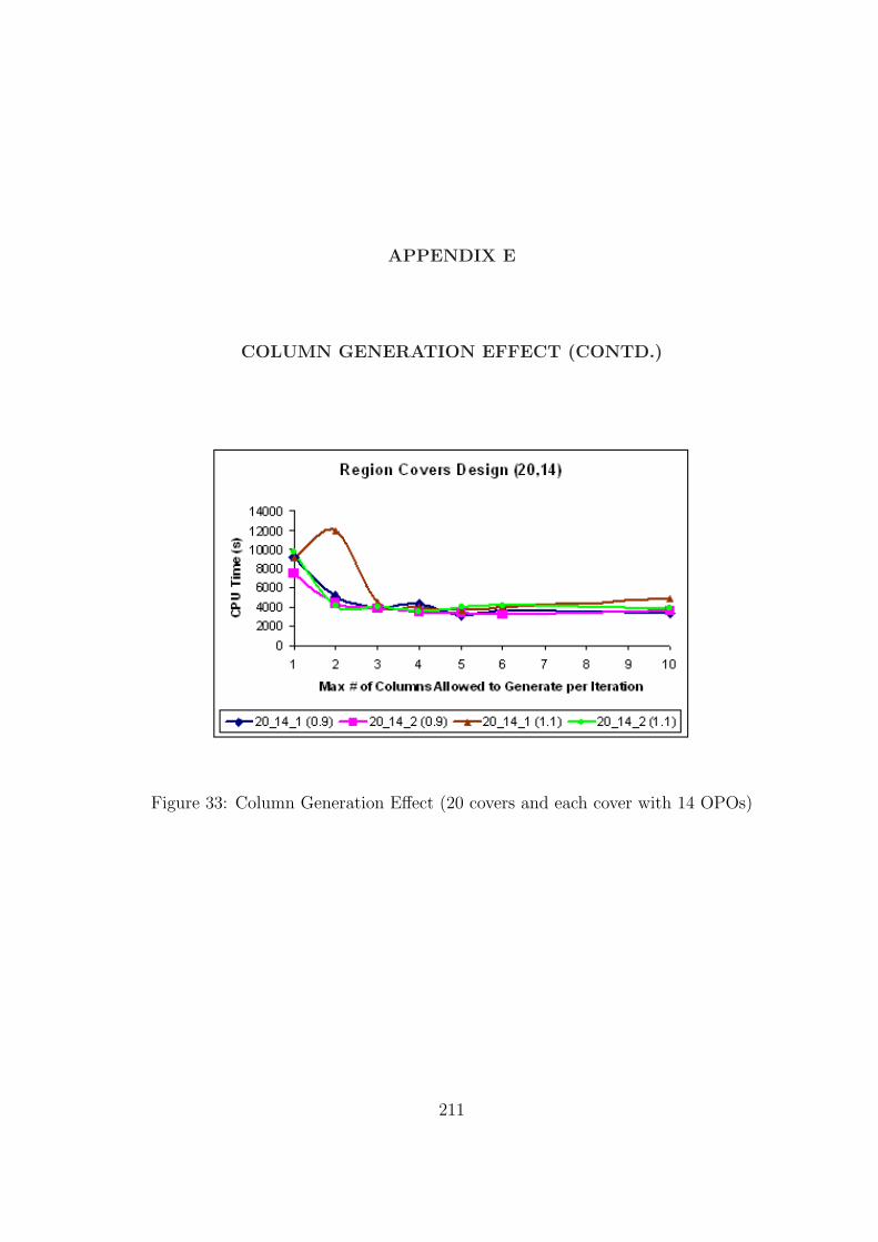
APPENDIX E
COLUMN GENERATION EFFECT (CONTD.)
Figure 33: Column Generation Effect (20 covers and each cover with 14 OPOs)
211
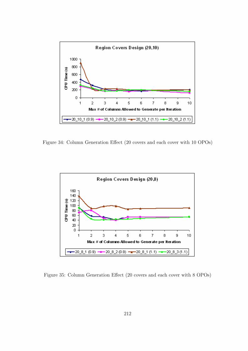
Figure 34: Column Generation Effect (20 covers and each cover with 10 OPOs)
Figure 35: Column Generation Effect (20 covers and each cover with 8 OPOs)
212
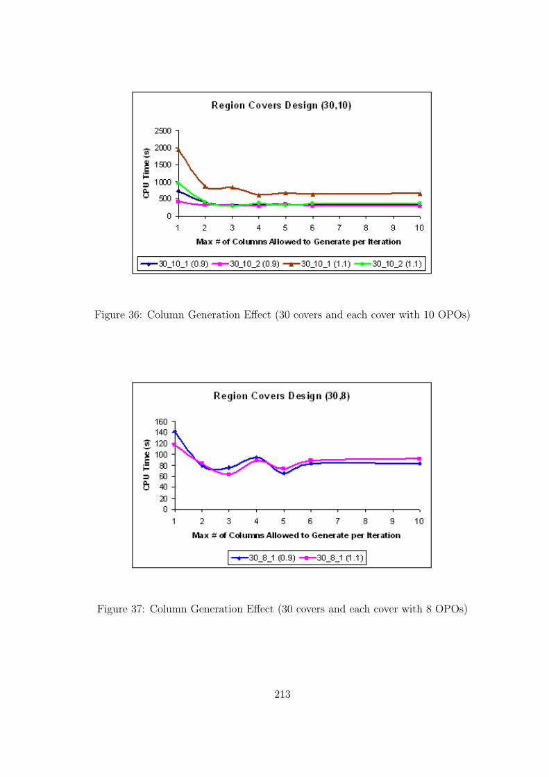
Figure 36: Column Generation Effect (30 covers and each cover with 10 OPOs)
Figure 37: Column Generation Effect (30 covers and each cover with 8 OPOs)
213

Figure 38: Column Generation Effect (25 covers and each cover with 12 OPOs)
Figure 39: Column Generation Effect (15 covers and each cover with 12 OPOs)
214

APPENDIX F
PRICING PROBLEM SOLUTION OPTION
215

Table 40: Pricing Problem Solution Options: Design (20,14)
Solution Options p0 = 0.9 p0 = 1.1
MIP Heuristic MIP # # # #
Instance Emphasis Frequency Gap CPU (s) Iters Cols CPU (s) Iters Cols
feasibility none 10−4 4702 23 1245 4071 20 1207
feasibility none 5% 3654 22 1218 3947 22 1257
feasibility none 10% 3355 21 1231 4178 22 1282
feasibility automatic 10−4 3800 20 1100 4412 21 1176
feasibility automatic 5% 3497 21 1163 4939 22 1164
feasibility automatic 10% 4841 24 1210 4592 22 1061
feasibility 1 10−4 12014 23 1170 14102 23 1127
feasibility 1 5% 12663 24 1202 10996 22 1114
feasibility 1 10% 11073 23 1157 13444 25 1140
feasibility 10 10−4 4831 23 1134 4637 21 1141
feasibility 10 5% 4734 23 1245 4450 21 1045
20 14 1 feasibility 10 10% 5247 24 1241 6227 24 1135
balance none 10−4 3448 26 934 3939 27 1060
balance none 5% 3022 24 988 2557 22 984
balance none 10% 2719 24 939 3300 24 966
balance automatic 10−4 3383 23 1095 4835 25 1167
balance automatic 5% 3254 23 1084 4773 26 1133
balance automatic 10% 3357 23 1094 4027 26 1135
balance 1 10−4 7334 22 1184 9517 23 1205
balance 1 5% 8595 24 1156 9657 25 1159
balance 1 10% 8351 24 1159 9031 24 1208
balance 10 10−4 3561 23 1078 4123 24 1145
balance 10 5% 3455 26 934 5505 27 1124
balance 10 10% 3850 23 1057 5021 26 1143
feasibility none 10−4 3175 22 1276 3480 22 1264
feasibility none 5% 3086 21 1153 3537 22 1241
feasibility none 10% 3071 21 1198 3864 23 1136
feasibility automatic 10−4 3570 21 1246 5221 24 1128
feasibility automatic 5% 4183 24 1094 4164 23 1109
feasibility automatic 10% 5168 26 1198 4409 24 1155
feasibility 1 10−4 10512 22 1065 12839 25 1178
feasibility 1 5% 10443 23 1200 13304 25 1225
feasibility 1 10% 14373 26 1146 13406 25 1089
feasibility 10 10−4 3902 22 1099 5004 22 1096
feasibility 10 5% 3177 22 1276 5010 23 1126
20 14 2 feasibility 10 10% 4672 23 1212 3890 22 1099
balance none 10−4 2970 26 1014 3197 24 944
balance none 5% 2959 26 977 2892 24 959
balance none 10% 2884 24 959 3398 25 993
balance automatic 10−4 3514 24 1072 3923 24 1098
balance automatic 5% 3289 24 1080 3723 25 1052
balance automatic 10% 3866 26 1137 3734 25 1135
balance 1 10−4 9665 25 1158 9321 24 1208
balance 1 5% 8505 25 1189 10697 27 1253
balance 1 10% 7713 25 1144 8590 24 1124
balance 10 10−4 3559 25 1098 4505 25 1142
balance 10 5% 2964 26 1014 3969 24 1142
balance 10 10% 3334 24 1196 4310 25 1149
216

Table 41: Pricing Problem Solution Options: Design (20,10)
Solution Options p0 = 0.9 p0 = 1.1
MIP Heuristic MIP # # # #
Instance Emphasis Frequency Gap CPU (s) Iters Cols CPU (s) Iters Cols
feasibility none 10−4 129 18 748 163 19 695
feasibility none 5% 110 17 694 162 20 667
feasibility none 10% 129 18 731 151 19 671
feasibility automatic 10−4 185 20 646 162 18 655
feasibility automatic 5% 184 21 628 159 19 687
feasibility automatic 10% 173 20 683 168 19 660
feasibility 1 10−4 429 19 609 381 18 665
feasibility 1 5% 464 21 644 479 21 682
feasibility 1 10% 503 23 667 576 22 651
feasibility 10 10−4 235 21 691 198 19 704
feasibility 10 5% 173 19 645 205 21 653
20 10 1 feasibility 10 10% 211 21 709 197 20 635
balance none 10−4 167 23 595 219 23 565
balance none 5% 152 20 525 215 25 590
balance none 10% 158 21 572 158 21 576
balance automatic 10−4 209 20 660 206 19 653
balance automatic 5% 244 23 650 214 22 709
balance automatic 10% 225 21 633 223 21 620
balance 1 10−4 376 19 653 582 22 689
balance 1 5% 483 21 619 527 22 671
balance 1 10% 435 21 671 572 24 677
balance 10 10−4 223 21 671 203 18 596
balance 10 5% 214 21 662 269 24 717
balance 10 10% 193 20 608 268 23 665
feasibility none 10−4 123 19 675 126 18 673
feasibility none 5% 93 17 648 126 19 627
feasibility none 10% 157 22 7336 133 18 652
feasibility automatic 10−4 126 18 639 147 18 659
feasibility automatic 5% 117 18 706 157 19 642
feasibility automatic 10% 122 18 614 162 20 608
feasibility 1 10−4 388 20 675 349 18 632
feasibility 1 5% 354 20 626 427 20 632
feasibility 1 10% 411 21 644 526 23 645
feasibility 10 10−4 163 19 684 162 18 635
feasibility 10 5% 169 20 642 174 19 582
20 10 2 feasibility 10 10% 156 19 600 157 19 623
balance none 10−4 142 21 577 167 23 566
balance none 5% 149 22 547 141 19 506
balance none 10% 144 21 572 154 20 528
balance automatic 10−4 121 16 622 154 18 592
balance automatic 5% 180 20 613 151 18 577
balance automatic 10% 195 21 650 185 21 614
balance 1 10−4 348 19 696 326 19 669
balance 1 5% 399 21 669 334 19 619
balance 1 10% 303 19 624 437 23 677
balance 10 10−4 205 21 697 175 19 596
balance 10 5% 204 22 662 173 19 599
balance 10 10% 197 21 584 210 22 637
217
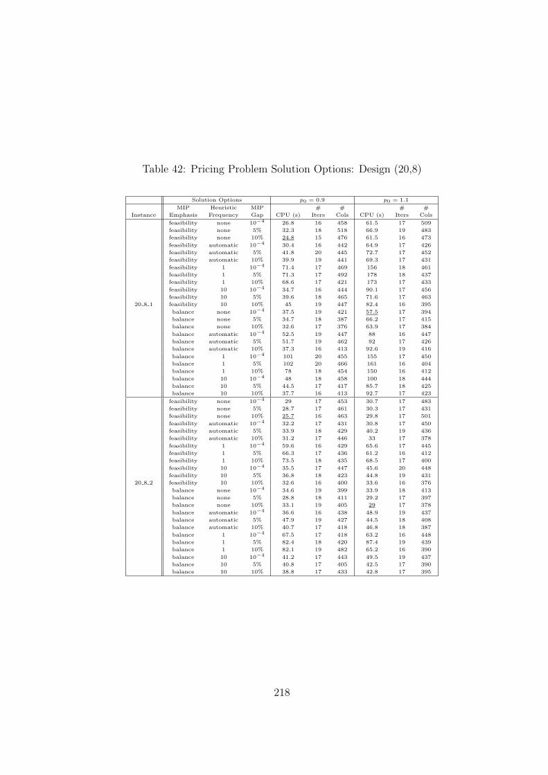
Table 42: Pricing Problem Solution Options: Design (20,8)
Solution Options p0 = 0.9 p0 = 1.1
MIP Heuristic MIP # # # #
Instance Emphasis Frequency Gap CPU (s) Iters Cols CPU (s) Iters Cols
feasibility none 10−4 26.8 16 458 61.5 17 509
feasibility none 5% 32.3 18 518 66.9 19 483
feasibility none 10% 24.8 15 476 61.5 16 473
feasibility automatic 10−4 30.4 16 442 64.9 17 426
feasibility automatic 5% 41.8 20 445 72.7 17 452
feasibility automatic 10% 39.9 19 441 69.3 17 431
feasibility 1 10−4 71.4 17 469 156 18 461
feasibility 1 5% 71.3 17 492 178 18 437
feasibility 1 10% 68.6 17 421 173 17 433
feasibility 10 10−4 34.7 16 444 90.1 17 456
feasibility 10 5% 39.6 18 465 71.6 17 463
20 8 1 feasibility 10 10% 45 19 447 82.4 16 395
balance none 10−4 37.5 19 421 57.5 17 394
balance none 5% 34.7 18 387 66.2 17 415
balance none 10% 32.6 17 376 63.9 17 384
balance automatic 10−4 52.5 19 447 88 16 447
balance automatic 5% 51.7 19 462 92 17 426
balance automatic 10% 37.3 16 413 92.6 19 416
balance 1 10−4 101 20 455 155 17 450
balance 1 5% 102 20 466 161 16 404
balance 1 10% 78 18 454 150 16 412
balance 10 10−4 48 18 458 100 18 444
balance 10 5% 44.5 17 417 85.7 18 425
balance 10 10% 37.7 16 413 92.7 17 423
feasibility none 10−4 29 17 453 30.7 17 483
feasibility none 5% 28.7 17 461 30.3 17 431
feasibility none 10% 25.7 16 463 29.8 17 501
feasibility automatic 10−4 32.2 17 431 30.8 17 450
feasibility automatic 5% 33.9 18 429 40.2 19 436
feasibility automatic 10% 31.2 17 446 33 17 378
feasibility 1 10−4 59.6 16 429 65.6 17 445
feasibility 1 5% 66.3 17 436 61.2 16 412
feasibility 1 10% 73.5 18 435 68.5 17 400
feasibility 10 10−4 35.5 17 447 45.6 20 448
feasibility 10 5% 36.8 18 423 44.8 19 431
20 8 2 feasibility 10 10% 32.6 16 400 33.6 16 376
balance none 10−4 34.6 19 399 33.9 18 413
balance none 5% 28.8 18 411 29.2 17 397
balance none 10% 33.1 19 405 29 17 378
balance automatic 10−4 36.6 16 438 48.9 19 437
balance automatic 5% 47.9 19 427 44.5 18 408
balance automatic 10% 40.7 17 418 46.8 18 387
balance 1 10−4 67.5 17 418 63.2 16 448
balance 1 5% 82.4 18 420 87.4 19 439
balance 1 10% 82.1 19 482 65.2 16 390
balance 10 10−4 41.2 17 443 49.5 19 437
balance 10 5% 40.8 17 405 42.5 17 390
balance 10 10% 38.8 17 433 42.8 17 395
218
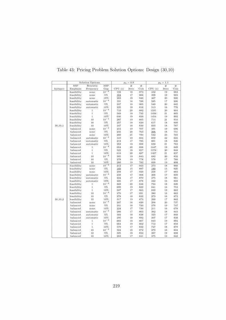
Table 43: Pricing Problem Solution Options: Design (30,10)
Solution Options p0 = 0.9 p0 = 1.1
MIP Heuristic MIP # # # #
Instance Emphasis Frequency Gap CPU (s) Iters Cols CPU (s) Iters Cols
feasibility none 10−4 193 18 973 432 19 984
feasibility none 5% 184 17 906 399 19 923
feasibility none 10% 203 18 946 467 20 900
feasibility automatic 10−4 191 16 789 585 17 906
feasibility automatic 5% 227 18 905 549 20 845
feasibility automatic 10% 225 18 816 513 16 776
feasibility 1 10−4 710 20 882 1331 20 904
feasibility 1 5% 569 18 735 1456 21 865
feasibility 1 10% 646 19 839 1454 19 802
feasibility 10 10−4 287 19 865 714 21 910
feasibility 10 5% 257 18 820 617 18 900
30 10 1 feasibility 10 10% 247 18 830 603 18 787
balanced none 10−4 215 19 707 491 19 696
balanced none 5% 235 20 763 396 18 751
balanced none 10% 260 21 780 542 23 793
balanced automatic 10−4 310 19 884 659 22 845
balanced automatic 5% 218 17 795 601 18 826
balanced automatic 10% 262 19 808 639 21 783
balanced 1 10−4 664 20 888 1447 19 849
balanced 1 5% 522 18 857 1376 20 848
balanced 1 10% 619 20 887 1407 21 837
balanced 10 10−4 305 19 843 682 20 832
balanced 10 5% 278 19 778 578 17 780
balanced 10 10% 280 19 783 609 19 808
feasibility none 10−4 212 17 943 273 18 966
feasibility none 5% 169 15 897 189 15 925
feasibility none 10% 208 17 929 238 17 883
feasibility automatic 10−4 238 17 908 268 17 909
feasibility automatic 5% 224 17 870 275 18 961
feasibility automatic 10% 225 17 878 242 16 802
feasibility 1 10−4 869 20 848 724 18 829
feasibility 1 5% 699 19 822 641 16 753
feasibility 1 10% 597 17 863 822 19 862
feasibility 10 10−4 270 17 921 280 16 862
feasibility 10 5% 278 18 832 279 16 872
30 10 2 feasibility 10 10% 317 19 873 290 17 862
balanced none 10−4 207 16 629 298 20 737
balanced none 5% 241 18 720 276 19 747
balanced none 10% 224 17 730 211 16 678
balanced automatic 10−4 286 17 863 362 18 843
balanced automatic 5% 302 18 838 323 17 849
balanced automatic 10% 295 18 892 307 17 838
balanced 1 10−4 665 18 867 843 19 894
balanced 1 5% 664 19 862 712 17 858
balanced 1 10% 579 17 832 727 18 879
balanced 10 10−4 324 18 872 279 16 834
balanced 10 5% 325 18 833 387 19 808
balanced 10 10% 283 17 841 375 19 842
219
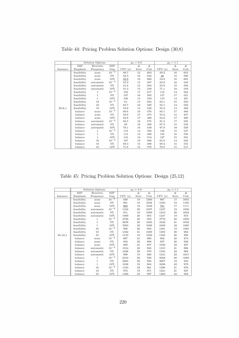
Table 44: Pricing Problem Solution Options: Design (30,8)
Solution Options p0 = 0.9 p0 = 1.1
MIP Heuristic MIP # # # #
Instance Emphasis Frequency Gap CPU (s) Iters Cols CPU (s) Iters Cols
feasibility none 10−4 49.7 15 663 59.2 16 653
feasibility none 5% 52.3 16 642 48 15 596
feasibility none 10% 50.9 16 606 53.8 16 665
feasibility automatic 10−4 55.9 15 567 63.6 16 544
feasibility automatic 5% 51.8 15 504 53.9 15 556
feasibility automatic 10% 51.3 15 548 71.1 18 549
feasibility 1 10−4 156 17 617 116 14 564
feasibility 1 5% 137 16 505 157 17 521
feasibility 1 10% 108 14 549 110 14 491
feasibility 10 10−4 61 15 650 64.1 15 550
feasibility 10 5% 63.7 16 520 54.1 14 522
30 8 1 feasibility 10 10% 52.8 14 522 55.2 14 492
balance none 10−4 60.6 16 476 64.1 17 484
balance none 5% 59.9 17 475 55.2 15 457
balance none 10% 62.6 17 488 64.8 17 490
balance automatic 10−4 82.5 16 575 91.5 17 525
balance automatic 5% 92 18 506 67.3 15 534
balance automatic 10% 78.1 16 548 97.8 18 529
balance 1 10−4 119 14 556 136 15 547
balance 1 5% 113 14 490 145 16 530
balance 1 10% 116 14 514 127 15 501
balance 10 10−4 107 19 566 65.6 14 522
balance 10 5% 69.3 15 498 69.4 15 534
balance 10 10% 71.8 15 576 70.9 15 517
Table 45: Pricing Problem Solution Options: Design (25,12)
Solution Options p0 = 0.9 p0 = 1.1
MIP Heuristic MIP # # # #
Instance Emphasis Frequency Gap CPU (s) Iters Cols CPU (s) Iters Cols
feasibility none 10−4 928 19 1200 867 17 1055
feasibility none 5% 901 19 1058 1033 19 1105
feasibility none 10% 809 18 1049 781 17 1111
feasibility automatic 10−4 1162 20 1037 1247 19 1036
feasibility automatic 5% 911 19 1000 1213 20 1024
feasibility automatic 10% 1069 20 955 1247 19 919
feasibility 1 10−4 2720 20 952 3779 20 1002
feasibility 1 5% 2658 20 1023 3432 21 1042
feasibility 1 10% 3303 22 1009 3458 22 1085
feasibility 10 10−4 998 20 956 1381 19 1065
feasibility 10 5% 1322 21 1020 1303 20 962
25 12 1 feasibility 10 10% 1133 19 1022 1325 20 999
balance none 10−4 887 21 880 902 20 874
balance none 5% 932 22 909 937 20 849
balance none 10% 869 21 857 1049 22 827
balance automatic 10−4 1214 22 924 1315 21 966
balance automatic 5% 1028 20 970 1345 22 968
balance automatic 10% 999 19 980 1241 22 1017
balance 1 10−4 2410 20 936 2568 20 1069
balance 1 5% 2265 20 994 2067 18 934
balance 1 10% 1938 19 964 3236 22 979
balance 10 10−4 1193 22 961 1290 21 979
balance 10 5% 972 19 971 1241 21 927
balance 10 10% 1406 23 997 1484 23 958
220

Table 46: Pricing Problem Solution Options: Design (15,12)
Solution Options p0 = 0.9 p0 = 1.1
MIP Heuristic MIP # # # #
Instance emphasis frequency gap CPU (s) Iters Cols CPU (s) Iters Cols
feasibility none default 920 23 797 712 21 788
feasibility none 5% 784 23 802 1046 24 833
feasibility none 10% 863 23 809 793 22 781
feasibility automatic default 846 23 690 861 23 734
feasibility automatic 5% 1201 27 792 967 23 735
feasibility automatic 10% 899 24 733 989 24 790
feasibility 1 default 2723 25 747 2998 25 707
feasibility 1 5% 2920 26 810 2958 25 695
feasibility 1 10% 3134 25 724 3354 26 705
feasibility 10 default 1213 26 766 1015 23 742
feasibility 10 5% 1014 24 737 1344 26 743
15 12 1 feasibility 10 10% 955 23 724 1098 24 794
optimality none default 959 28 694 1063 28 677
optimality none 5% 687 25 640 885 26 687
optimality none 10% 811 28 707 911 27 626
optimality automatic default 1050 27 712 1062 26 739
optimality automatic 5% 909 25 746 889 24 688
optimality automatic 10% 1061 27 757 1077 27 728
optimality 1 default 1867 23 773 2383 25 754
optimality 1 5% 2394 26 801 2326 27 789
optimality 1 10% 2137 26 783 2745 27 807
optimality 10 default 859 25 739 1137 26 717
optimality 10 5% 757 23 702 1176 27 749
optimality 10 10% 1155 27 789 1058 24 709
221

APPENDIX G
STRENGTH OF CLASS I VALID INEQUALITY
222

Table 47: Strength of Class I Valid Inequalities (RPP 0 0 2)
National Cardinality LP Duality Gap (%) CPU Time (s)Flow li0 Value O1 O2 O3 O4 O1 O2 O3 O4
3 21.8 20.1 16.0 14.2 1.22 1.18 1.21 1.234 10.9 8.1 5.1 3.8 1.83 1.09 1.34 0.395 7.6 4.9 3.0 2.6 1.38 0.68 1.16 0.616 8.6 5.0 3.2 2.7 1.70 1.45 1.35 1.257 8.2 4.7 3.0 2.5 1.64 1.52 1.49 1.39
200 8 7.8 4.1 2.9 2.3 1.86 1.77 0.93 1.389 7.5 3.6 2.8 2.0 2.67 1.97 1.83 1.9310 7.3 3.0 2.6 1.7 2.30 3.31 1.92 3.6211 0 0 0 0 0.23 0.39 0.25 0.3812 0.8 0 0.1 0 0.31 0.33 0.37 0.3713 8.9 0.1 0.2 0 0.70 0.54 0.61 0.533 14.9 13.6 12.3 11.0 1.15 1.47 1.24 1.174 5.9 3.9 3.1 2.1 1.10 1.08 0.35 0.375 3.1 1.6 1.4 1.0 0.73 0.35 0.22 0.376 4.3 1.7 1.7 1.2 1.02 0.66 1.19 0.727 4.1 1.6 1.6 1.1 1.38 0.65 0.81 0.88
100 8 3.8 1.2 1.5 0.8 1.46 0.82 1.33 0.969 3.6 0.8 1.4 0.6 1.27 1.08 1.75 0.9110 3.5 0.5 1.3 0.4 1.61 1.28 0.64 1.1011 0 0 0 0 0.22 0.44 0.19 0.4412 0 0 0 0 0.16 0.29 0.17 0.3713 0.7 0 0 0 1.62 0.25 1.49 0.333 7.6 6.5 6.6 5.7 0.89 0.94 1.37 0.744 3.3 1.8 1.9 1.2 0.78 0.51 0.33 0.665 0.9 0.2 0.5 0.2 0.38 0.28 0.22 0.266 2.1 0.5 0.8 0.4 0.50 0.47 0.74 0.407 2.0 0.5 0.8 0.4 0.52 0.63 0.66 0.53
50 8 1.8 0.3 0.7 0.2 0.63 0.55 0.80 0.579 1.6 0.1 0.6 0.1 1.08 0.58 0.62 0.5310 1.6 0.1 0.5 0.1 0.47 0.63 0.33 0.6311 0 0 0 0 0.18 0.33 0.18 0.3312 0 0 0 0 0.18 0.24 0.18 0.2313 0 0 0 0 0.19 0.28 0.20 0.283 2.7 1.9 2.3 1.7 0.26 0.21 0.3 0.24 2.2 1.1 1.4 0.9 0.31 0.96 0.7 0.45 0.2 0 0.1 0 0.21 0.13 0.2 0.16 1.3 0.2 0.5 0.2 0.38 0.32 0.8 0.37 1.2 0.2 0.4 0.2 0.43 0.40 0.9 0.4
30 8 1.0 0.1 0.4 0.1 0.45 0.40 0.6 0.49 0.8 0.0 0.3 0.0 0.71 0.30 0.3 0.310 0.8 0.0 0.3 0.0 0.32 0.51 0.3 0.511 0 0 0 0 0.16 0.31 0.2 0.312 0 0 0 0 0.17 0.21 0.2 0.213 0 0 0 0 0.19 0.38 0.2 0.23 0.6 0.3 0.5 0.3 0.17 0.18 0.16 0.204 1.7 0.9 1.2 0.8 0.67 0.41 0.32 0.345 0 0 0 0 0.11 0.13 0.11 0.126 0.8 0.1 0.3 0.1 0.38 0.30 0.43 0.297 0.8 0.1 0.3 0.1 0.39 0.36 0.57 0.35
20 8 0.6 0.0 0.2 0.0 0.26 0.32 0.38 0.329 0.4 0 0.1 0 0.28 0.22 0.32 0.2110 0.4 0.0 0.1 0.0 0.33 0.26 0.35 0.2511 0 0 0 0 0.17 0.31 0.17 0.2912 0 0 0 0 0.17 0.21 0.18 0.2013 0 0 0 0 0.20 0.22 0.20 0.22
223

Table 48: Strength of Class I Valid Inequalities (Contd.) (RPP 0 0 2)
National Cardinality LP Duality Gap (%) CPU Time (s)Flow li0 Value O1 O2 O3 O4 O1 O2 O3 O4
3 0 0 0 0 0.08 0.11 0.09 0.114 1.2 0.9 0.9 0.8 0.72 0.37 0.32 0.745 0 0 0 0 0.11 0.12 0.12 0.116 0.4 0.1 0.1 0.1 0.25 0.29 0.41 0.297 0.3 0.0 0.1 0.0 0.27 0.21 0.46 0.21
10 8 0.1 0.0 0.1 0.0 0.26 0.20 0.35 0.209 0 0 0 0 0.12 0.16 0.13 0.1510 0.0 0 0.0 0 0.19 0.19 0.20 0.1911 0 0 0 0 0.15 0.23 0.16 0.2312 0 0 0 0 0.17 0.20 0.18 0.2013 0 0 0 0 0.18 0.23 0.20 0.223 0 0 0 0 0.08 0.11 0.09 0.114 0.5 0.4 0.4 0.4 0.20 0.25 0.22 0.255 0 0 0 0 0.10 0.12 0.11 0.126 0.2 0.0 0.0 0.0 0.24 0.18 0.32 0.187 0.1 0 0.0 0 0.26 0.16 0.37 0.15
5 8 0 0 0 0 0.12 0.15 0.12 0.149 0 0 0 0 0.13 0.16 0.13 0.1510 0 0 0 0 0.13 0.20 0.14 0.1911 0 0 0 0 0.14 0.19 0.15 0.1912 0 0 0 0 0.18 0.21 0.17 0.2013 0 0 0 0 0.18 0.22 0.19 0.213 0 0 0 0 0.08 0.11 0.09 0.114 0.1 0.1 0.1 0.1 0.20 0.26 0.21 0.115 0 0 0 0 0.09 0.12 0.10 0.126 0.1 0 0.0 0 0.23 0.14 0.27 0.127 0.1 0 0.0 0 0.24 0.15 0.31 0.15
3 8 0 0 0 0 0.13 0.16 0.12 0.159 0 0 0 0 0.13 0.15 0.12 0.1510 0 0 0 0 0.13 0.18 0.14 0.1711 0 0 0 0 0.15 0.18 0.15 0.1812 0 0 0 0 0.17 0.20 0.17 0.2013 0 0 0 0 0.18 0.20 0.19 0.213 0 0 0 0 0.08 0.11 0.08 0.114 0 0 0 0 0.09 0.11 0.09 0.105 0 0 0 0 0.09 0.12 0.09 0.126 0.0 0 0.0 0 0.23 0.12 0.20 0.127 0.0 0 0.0 0 0.25 0.15 0.17 0.14
2 8 0 0 0 0 0.11 0.15 0.11 0.149 0 0 0 0 0.12 0.15 0.13 0.1510 0 0 0 0 0.13 0.17 0.13 0.1711 0 0 0 0 0.14 0.18 0.15 0.1812 0 0 0 0 0.16 0.20 0.16 0.2013 0 0 0 0 0.17 0.21 0.19 0.203 0 0 0 0 0.08 0.10 0.09 0.104 0 0 0 0 0.10 0.11 0.09 0.115 0 0 0 0 0.09 0.12 0.10 0.116 0.0 0 0.0 0 0.22 0.12 0.14 0.127 0.0 0 0.0 0 0.15 0.14 0.16 0.13
1 8 0 0 0 0 0.11 0.15 0.11 0.149 0 0 0 0 0.12 0.16 0.12 0.1510 0 0 0 0 0.13 0.17 0.13 0.1611 0 0 0 0 0.14 0.19 0.15 0.1912 0 0 0 0 0.15 0.19 0.15 0.1813 0 0 0 0 0.19 0.21 0.18 0.21
224
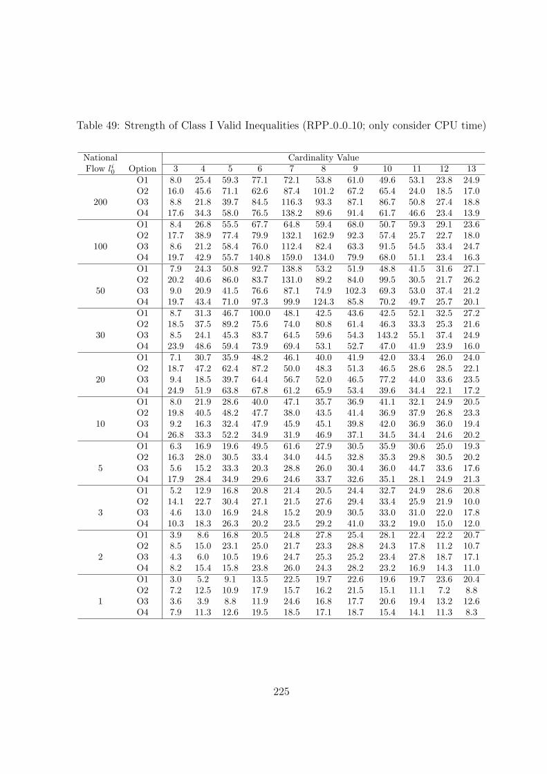
Table 49: Strength of Class I Valid Inequalities (RPP 0 0 10; only consider CPU time)
National Cardinality ValueFlow li0 Option 3 4 5 6 7 8 9 10 11 12 13
O1 8.0 25.4 59.3 77.1 72.1 53.8 61.0 49.6 53.1 23.8 24.9O2 16.0 45.6 71.1 62.6 87.4 101.2 67.2 65.4 24.0 18.5 17.0
200 O3 8.8 21.8 39.7 84.5 116.3 93.3 87.1 86.7 50.8 27.4 18.8O4 17.6 34.3 58.0 76.5 138.2 89.6 91.4 61.7 46.6 23.4 13.9O1 8.4 26.8 55.5 67.7 64.8 59.4 68.0 50.7 59.3 29.1 23.6O2 17.7 38.9 77.4 79.9 132.1 162.9 92.3 57.4 25.7 22.7 18.0
100 O3 8.6 21.2 58.4 76.0 112.4 82.4 63.3 91.5 54.5 33.4 24.7O4 19.7 42.9 55.7 140.8 159.0 134.0 79.9 68.0 51.1 23.4 16.3O1 7.9 24.3 50.8 92.7 138.8 53.2 51.9 48.8 41.5 31.6 27.1O2 20.2 40.6 86.0 83.7 131.0 89.2 84.0 99.5 30.5 21.7 26.2
50 O3 9.0 20.9 41.5 76.6 87.1 74.9 102.3 69.3 53.0 37.4 21.2O4 19.7 43.4 71.0 97.3 99.9 124.3 85.8 70.2 49.7 25.7 20.1O1 8.7 31.3 46.7 100.0 48.1 42.5 43.6 42.5 52.1 32.5 27.2O2 18.5 37.5 89.2 75.6 74.0 80.8 61.4 46.3 33.3 25.3 21.6
30 O3 8.5 24.1 45.3 83.7 64.5 59.6 54.3 143.2 55.1 37.4 24.9O4 23.9 48.6 59.4 73.9 69.4 53.1 52.7 47.0 41.9 23.9 16.0O1 7.1 30.7 35.9 48.2 46.1 40.0 41.9 42.0 33.4 26.0 24.0O2 18.7 47.2 62.4 87.2 50.0 48.3 51.3 46.5 28.6 28.5 22.1
20 O3 9.4 18.5 39.7 64.4 56.7 52.0 46.5 77.2 44.0 33.6 23.5O4 24.9 51.9 63.8 67.8 61.2 65.9 53.4 39.6 34.4 22.1 17.2O1 8.0 21.9 28.6 40.0 47.1 35.7 36.9 41.1 32.1 24.9 20.5O2 19.8 40.5 48.2 47.7 38.0 43.5 41.4 36.9 37.9 26.8 23.3
10 O3 9.2 16.3 32.4 47.9 45.9 45.1 39.8 42.0 36.9 36.0 19.4O4 26.8 33.3 52.2 34.9 31.9 46.9 37.1 34.5 34.4 24.6 20.2O1 6.3 16.9 19.6 49.5 61.6 27.9 30.5 35.9 30.6 25.0 19.3O2 16.3 28.0 30.5 33.4 34.0 44.5 32.8 35.3 29.8 30.5 20.2
5 O3 5.6 15.2 33.3 20.3 28.8 26.0 30.4 36.0 44.7 33.6 17.6O4 17.9 28.4 34.9 29.6 24.6 33.7 32.6 35.1 28.1 24.9 21.3O1 5.2 12.9 16.8 20.8 21.4 20.5 24.4 32.7 24.9 28.6 20.8O2 14.1 22.7 30.4 27.1 21.5 27.6 29.4 33.4 25.9 21.9 10.0
3 O3 4.6 13.0 16.9 24.8 15.2 20.9 30.5 33.0 31.0 22.0 17.8O4 10.3 18.3 26.3 20.2 23.5 29.2 41.0 33.2 19.0 15.0 12.0O1 3.9 8.6 16.8 20.5 24.8 27.8 25.4 28.1 22.4 22.2 20.7O2 8.5 15.0 23.1 25.0 21.7 23.3 28.8 24.3 17.8 11.2 10.7
2 O3 4.3 6.0 10.5 19.6 24.7 25.3 25.2 23.4 27.8 18.7 17.1O4 8.2 15.4 15.8 23.8 26.0 24.3 28.2 23.2 16.9 14.3 11.0O1 3.0 5.2 9.1 13.5 22.5 19.7 22.6 19.6 19.7 23.6 20.4O2 7.2 12.5 10.9 17.9 15.7 16.2 21.5 15.1 11.1 7.2 8.8
1 O3 3.6 3.9 8.8 11.9 24.6 16.8 17.7 20.6 19.4 13.2 12.6O4 7.9 11.3 12.6 19.5 18.5 17.1 18.7 15.4 14.1 11.3 8.3
225

APPENDIX H
A SPECIAL CASE OF RPP=(S): UNIMODALITY
Figure 40: Illustration of Unimodality (li0 = 200, 100, 50, 30, 20)
226
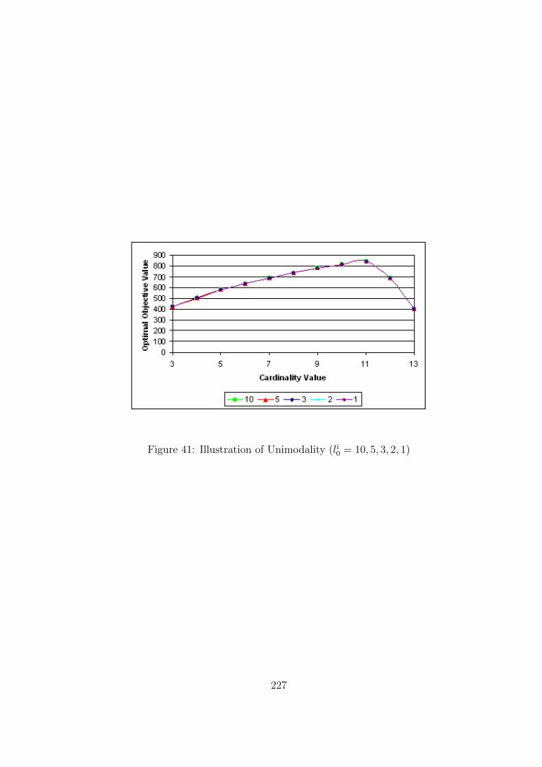
Figure 41: Illustration of Unimodality (li0 = 10, 5, 3, 2, 1)
227

BIBLIOGRAPHY
[1] Bill 921. South Carolina General Assembly (112th Session, 1997 - 1998).
[2] J. Abara. Applying integer linear programming to the fleet assignment problem. In-terfaces, 19(4):20–28, 1989.
[3] R. Adam, H. Bismuth, T. Diamond, B. Ducot, M. Morino, I. Astarcioglu, M. Johann,D. Azoulay, L. Chiche, and Y. M. Bao. Effect of extended cold ischaemia with UWsolution on graft function after liver transplantation. Lancet, 340:1373–1376, 1992.
[4] Y. Agarwal, K. Mathur, and H. M. Salkin. A set-partitioning-based exact algorithmfor the vehicle routing problem. Networks, 19:731–749, 1989.
[5] J. H. Ahn and J. C. Hornberger. Involving patients in the cadaveric kidney transplantallocation process: A decision-theoretic perspective. Management Science, 42(5):629–641, 1996.
[6] O. Alagoz. Optimal Policies for the Acceptance of Living- and Cadaveric-Donor Livers.PhD thesis, University of Pittsburgh, Pittsburgh, PA, 2004.
[7] O. Alagoz, L. M. Maillart, A. J. Schaefer, and M. S. Roberts. The optimal timing ofliving-donor liver transplantation. Management Science, 50(10):1420–1430, 2004.
[8] O. Alagoz, L. M. Maillart, A. J. Schaefer, and M. S. Roberts. Determining the accep-tance of cadaveric livers using an implicit model of the waiting list, 2005. Conditionallyaccepted at Operations Research.
[9] O. Alagoz, M. S. Roberts, C. L. Bryce, A. J. Schaefer, J. Chang, and D. C. Angus.Incorporating biological natural history in simulation models: Empiric estimates of theprogression of end-stage liver disease. Medical Decision Making, 25(6):620–632, 2005.
[10] O. Alagoz, A. J. Schaefer, and M. S. Roberts. Optimization in organ allocation, 2005.To appear in Handbook of Optimization in Medicine, P. Pardalos and E. Romeijn, eds.Kluwer Academic Publishers.
[11] R. Anbil, J. J. Forrest, and W. R. Pulleyblank. Column generation and the airlinecrew pairing problem. In Proceedings of the International Congress of Mathematics,Berlin, Germany, pages 677–686, 1998.
228
[12] R. Anbil, R. Tanga, and E. L. Johnson. A global approach to crew-pairing optimization.IBM Systems Journal, 31:71–78, 1992.
[13] E. Andersson, E. Housos, N. Kohl, and D. Wedelin. Crew pairing optimization. InG. Yu, editor, Operations Research in the Airline Industry, pages 228 – 258. KluwerAcademic Publishers, Boston, MA, 1997.
[14] L. H. Appelgren. A column generation algorithm for a ship scheduling problem. Trans-portation Science, 3:53–68, 1969.
[15] M. A. Bailey. Economic issues in organ substitution technology. In D. Mathieu, edi-tor, Organ Substitution Technology: Ethical, Legal and Public Policy Issues. WestviewPress, Boulder, CO, 1988.
[16] E. Balas and M. Padberg. Set partitioning: A survey. SIAM Review, 18:710–760, 1976.
[17] F. Barahona and R. Anbil. The volume algorithm: Producing primal solutions with asubgradient method. Mathematical Programming, 87(3):385–399, 2000.
[18] C. Barnhart, N. Boland, L. W. Clarke, E. L. Johnson, G. L. Nemhauser, and R. G.Shenoi. Flight string models for aircraft routing and scheduling. Transportation Sci-ence, 32(3):208–220, 1998.
[19] C. Barnhart, C. A. Hane, E. L. Johnson, and G. Sigismondi. An alternative formulationand solution strategy for multi-commodity network flow problems. TelecommunicationsSystems, 3:239–258, 1995.
[20] C. Barnhart, C. A. Hane, and P. H. Vance. Integer multicommodity flow problems.Lecture Notes in Economics and Mathematical Systems, 450:17–31, 1997.
[21] C. Barnhart, C. A. Hane, and P. H. Vance. Using branch-and-price-and-cut to solveorigin-destination integer multicommodity network flow problems. Operations Re-search, 48(3):318–326, 2000.
[22] C. Barnhart, E. L. Johnson, G. L. Nemhauser, M. W. P. Savelsbergh, and P. H. Vance.Branch-and-price: Column generation for solving huge integer programs. OperationsResearch, 46(3):316–329, 1998.
[23] C. Barnhart, T. S. Kniker, and M. Lohatepanont. Itinerary-based airline fleet assign-ment. Transportation Science, 36(2):199–217, 2002.
[24] C. Barnhart and R. R. Schneur. Air network design for express shipment service.Operations Research, 44(6):852–863, 1996.
[25] H. Ben Amor. Stabilisation de l’Algorithme de Generation de Colonnes. PhD thesis,Ecole Polytechnique de Montreal, Montreal, Canada, 2002.
229
[26] J. M. Benedict. Three Hierarchical Objective Models Which Incorporate the Conceptof Excess Coverage to Locate EMS Vehicles or Hospitals. PhD thesis, NorthwesternUniversity, Evanston, IL, 1983.
[27] M. A. Berge and C. Hopperstad. Demand driven dispatch: A method for dynamicaircraft capacity assignment, models, and algorithms. Operations Research, 41(1):153–168, 1993.
[28] R. E. Bixby. Solving real-world linear programs: A decade and more of progress.Operations Research, 50(1):3–15, 2002.
[29] R. E. Bixby, J. W. Gregory, I. J. Lustig, R. E. Marsten, and D. F. Shano. Verylarge-scale linear programming: A case study in combining interior point and simplexmethods. Operations Research, 40(5):885–897, 1992.
[30] K. Bjoro, B. G. Ericzon, P. Kirkegaard, K. Hockerstedt, G. Soderdahl, M. Olausson,A. Foss, L. E. Schmidt, H. Isoniemi, B. Brandsaeter, and S. Friman. Highly urgent livertransplantation: Possible impact of donor-recipient ABO matching on the outcomeafter transplantation. Transplantation, 75(3):347–353, 2003.
[31] R. Borndorfer, M. Grotschel, and A. Lobel. Duty scheduling in public transit. InW. Jager and H.-J. Krebs, editors, Mathematics – Key Technology for the Future,pages 653–674. Springer-Verlag, Berlin, Germany, 2003.
[32] E. Boros and P. Hammer. Pseudo-boolean optimization. Discrete Applied Mathematics,123(1-3):155–225, 2002.
[33] J.-M. Bourjolly, G. Laporte, and H. Mercure. A combinatorial column generationalgorithm for the maximum stable set problem. Operations Research Letters, 20(1):21–29, 1997.
[34] M. L. Brandeau and R. C. Larson. Extending and applying the hypercube queueingmodel to deploy ambulances in Boston. In E. Ignall and Swersey A. J., editors, Man-agement Science and the Delivery of Urban Service, TIMS Studies in the ManagementSciences Series. North-Holland/Elsevier, Amsterdam, The Netherlands, 1986.
[35] M. L. Brandeau, F. Sainfort, and W. P. Pierskalla. Operations Research and HealthCare: A Handbook of Methods and Applications. Kluwer Academic Publishers, Boston,MA, 2005.
[36] D. W. Brock. Ethical issues in recipient selection for organ transplantation. In D. Math-ieu, editor, Organ Substitution Technology: Ethical, Legal and Public Policy Issues.Westview Press, Boulder, CO, 1988.
[37] C. L. Bryce. Supplementary UNOS data set, 2005. Personal Correspondence.
[38] U.S. Census Bureau. GCT-PH1. Population, Housing Unit, Area, and Density: 2000.Available from http://www.census.gov.
230
[39] A. Caprara, M. Fischetti, and P. Toth. A heuristic method for the set covering problem.Operations Research, 47:730–743, 1999.
[40] A. Caprara, M. Fischetti, and P. Toth. Algorithms for the set covering problem. Annalsof Operations Research, 98:353–371, 2000.
[41] Y. M. Carson and R. Batta. Locating an ambulance on the Amherst campus of theState University of New York at Buffalo. Interfaces, 20:43–49, 1990.
[42] F. C. Chow and J. L. Hennessy. Register allocation by priority-based coloring. InProceedings of the ACM SIGPLAN 84 Symposium on Complier Construction, pages222–232, New York, NY, 1984. ACM.
[43] F. C. Chow and J. L. Hennessy. The priority-based coloring approach to registerallocation. ACM Transactions on Programming Languages and Systems, 12(4):501–536, 1990.
[44] H. D. Chu, E. Gelman, and E. L. Johnson. Solving large scale crew scheduling problems.European Journal of Operational Research, 97:260–268, 1997.
[45] V. Chvatal. Linear Programming. W. H. Freeman and Company, New York, NY, 1983.
[46] L. Clarke, C. Hane, E. Johnson, and G. Nemhauser. Maintenance and crew consider-ation in fleet assignment. Transportation Science, 30:249–260, 1996.
[47] COIN-OR. COIN-OR Documentation: Branch-Cut-Price Framework. Available fromhttp://www.coin-or.org/documentation.html.
[48] G. Cornuejols, M. Fisher, and G. Nemhauser. Location of bank accounts to optimizefloat: An analytic study of exact and approximation algorithms. Management Science,23:789–810, 1977.
[49] T. G. Crainic and J.-M. Rousseau. The column generation principle and the airlinecrew pairing problem. IFOR, 25(2):136–151, 1987.
[50] Y. Crama and A. G. Oerlemans. A column generation approach to job grouping forflexible manufacturing systems. European Journal of Operational Research, 78(1):58–80, 1994.
[51] G. B. Dantzig and A. R. Ferguson. The problem of routing – A mathematical solution.Technical Report AD604395, Federal Clearinghouse, Washington, D.C., 1954.
[52] G. B. Dantzig and P. Wolfe. Decomposition principle for linear programs. OperationsResearch, 8:101–111, 1960.
[53] M. S. Daskin. Application of an expected covering model to EMS system design.Decision Sciences, 13:416–439, 1982.
231

[54] M. S. Daskin. Network and Discrete Location: Models, Algorithms and Applications.Wiley, New York, NY, 1995.
[55] M. S. Daskin and L. K. Dean. Locations of health care facilities. In M. L. Brandeau,F. Sainfort, and W. P. Pierskalla, editors, Operations Research and Health Care: AHandbook of Methods and Applications. Kluwer Academic Publishers, Boston, MA,2005.
[56] M. S. Daskin and N. D. Panayotopoulos. A Lagrangian relaxation approach to assigningaircraft to routes in hub and spoke networks. Transportation Science, 23:91–99, 1989.
[57] M. S. Daskin and E. Stern. A hierarchical objective set covering model for EMS vehicledeployment. Transportation Science, 15:137–152, 1981.
[58] I. David and U. Yechiali. A time-dependent stopping problem with application to liveorgan transplants. Operations Research, 33(3):491–504, 1985.
[59] I. David and U. Yechiali. Sequential assignment match processes with arrivals of can-didates and offers. Probability in Engineering and Information Sciences, 4(4):413–430,1990.
[60] I. David and U. Yechiali. One-attribute sequential assignment match processes indiscrete time. Operations Research, 43(5):879–884, 1995.
[61] J. de Meester, M. Bogers, H. de Winter, J. Smits, L. Meester, M. Dekking, F. Lootsma,G. Persijn, and F. Muhlbacher. Which ABO-matching rule should be the decisivefactor in the choice between a highly urgent and an elective patient? TransplantationInternational, 15(8):431–435, 2002.
[62] C. C. de Souza. The Graph Equipartition Problem: Optimal Solutions, Extensionsand Applications. PhD thesis, Universite Catholique de Louvain, Louvain-la-Neuve,Belgium, 1993.
[63] D. de Werra. An introduction to timetabling. European Journal of Operational Re-search, 19(2):151–162, 1985.
[64] C. Derman, G. J. Lieberman, and S. M. Ross. A sequential stochastic assignmentproblem. Management Science, 18:349–355, 1972.
[65] G. Desaulniers, J. Desrosiers, Y. Dumas, M. M. Solomon, and F. Soumis. Daily aircraftrouting and scheduling. Management Science, 43(6):841–855, 1997.
[66] G. Desaulniers, J. Desrosiers, and M. M. Solomon. Accelerating strategies in columngeneration methods for vehicle routing and crew scheduling problems. In C. C. Ribeiroand P. Hansen, editors, Essays and Surveys in Metaheuristics, pages 309–324. Kluwer,Boston, MA, 2001.
232

[67] M. Desrochers, J. Desrosiers, and M. M. Solomon. A new optimization algorithm forthe vehicle routing problem with time windows. Operations Research, 40(2):342–354,1992.
[68] M. Desrochers and F. Soumis. A column generation approach to urban transit crewscheduling. Transportation Science, 23:1–13, 1989.
[69] J. Desrosiers. An overview of column generation. Talk in Seminar on “DiscreteMathematics and Applications” in the Department of Discrete Mathematics at Leib-niz Laboratory, Leibniz, France, on April 15th, 1999. Available from http://www-leibniz.imag.fr/DMD/sem/1999/indexe.html.
[70] J. Desrosiers, Y. Dumas, M. M. Solomon, and F. Soumis. Time constrained routing andscheduling. In M. O. Ball, T. L. Magnanti, C. L. Monma, and G. L. Nemhauser, edi-tors, Handbooks in Operations Research and Management Science, Volumn 8: NetworkRouting, pages 35–139. Elsevier, Amsterdam, The Netherlands, 1995.
[71] J. Desrosiers and M. E. Lubbecke. Selected topics in column generation. OperationsResearch, 53(6), 2005. In print.
[72] J. Desrosiers, F. Soumis, and M. Desrochers. Routing with time windows by columngeneration. Networks, 14:545–565, 1984.
[73] O. du Merle, D. Villeneuve, J. Desrosiers, and P. Hansen. Stabilized column generation.Discrete Mathematics, 194(1-3):229–237, 1999.
[74] Y. Dumas, J. Desrosiers, and F. Soumis. The pickup and delivery problem with timewindows. European Journal of Operational Research, 54:7–22, 1991.
[75] D. J. Eaton. Location techniques for emergency medical service vehicles: Volume I– An analytical framework for Austin, Texas. Technical report, University of Texas,Austin, Texas, 1979.
[76] D. J. Eaton, M. S. Daskin, D. Simmons, B. Bulloch, and G. Jansma. Determiningemergency medical service vehicle deployment in Austin, Texas. Interfaces, 15:96–108,1985.
[77] D. J. Eaton, H. M. Sanchez, R. R. Lantigua, and Morgan J. Determining ambu-lance deployment in Santo Domingo, Dominican Republic. Journal of the OperationsResearch Society, 37:113–126, 1986.
[78] M. Eben-Chaime, C. A. Tovey, and J. C. Ammons. Circuit partitioning via set parti-tioning and column generation. Operations Research, 44(1):65–76, 1996.
[79] M. Elf, C. Gutwenger, M. Junger, and G. Rinaldi. Branch-and-cut algorithms forcombinatorial optimization and their implementation in ABACUS. In M. Jungerand D. Naddef, editors, Computational Combinatorial Optimization, pages 157 – 222.Springer-Verlag, Berlin, Germany, 2001.
233
[80] I. Elhallaoui, D. Villeneuve, F. Soumis, and G. Desaulniers. Dynamic aggregation ofset-partitioning constraints in column generation. Operations Research, 53(4):632–645,2005.
[81] H. English, S. Pollard, C. Flamank, M. Belger, and R. Calne. The use of ABO-compatible mismatched in the UK. Transplantation International, 7(S1):S102–103,1994.
[82] A. Erdmann, A. Nolte, A. Noltemeier, and R. Schrader. Modeling and solving an airlineschedule generation problem. Annals of Operations Research, 107:117–142, 2001.
[83] R. W. Evans, D. L. Manninen, and F. B. Dong. An economic analysis of liver trans-plantation: Costs, insurance coverage and reimbursement. Gastroenterology Clinics ofNorth America, 22(2):451–473, 1993.
[84] A. A. Farley. A note on bounding a class of linear programming problems, includingcutting stock problems. Operations Research, 38(5):922–923, 1990.
[85] J. A. Fitzsimmons. A methodology for emergency ambulance. Management Science,19:627–636, 1973.
[86] National Center for Health Statistics (NCHS). National Vital Statistics Report –Deaths: Preliminary Data for 2002, 2004. NVSR Vol. 52, No. 13. Available fromhttp://www.cdc.gov/nchs/products/pubs/pubd/nvsr/nvsr.htm.
[87] COmputational INterface for Operations Research (COIN-OR). Available fromhttp://www.coin-or.org.
[88] United Network for Organ Sharing (UNOS). Available from http://www.unos.org.
[89] L. R. Ford and D. R. Fulkerson. A suggested computation for maximal multicommoditynetwork flows. Management Science, 5:97–101, 1958.
[90] J. J. Forrest and D. Goldfarb. Steepest-edge simplex algorithms for linear program-ming. Mathematical Programming, 57:341–374, 1992.
[91] R. L. Francis, L. F. McGinnis, and J. A. White. Facility Layout and Location: AnAnalytical Approach. Prentice Hall, Englewood Cliffs, NJ, 1992.
[92] H. Furukawa, S. Todo, O. Imventarza, A. Casavilla, Y. M. Wu, C. Scotti-Foglieni,B. Broznick, J. Bryant, R. Day, and T. E. Starzl. Effect of cold ischemia time on theearly outcome of human hepatic allografts preserved with UW solution. Transplanta-tion, 51(5):1000–1004, 1991.
[93] M. Galati. AAP BP: A COIN/BCP branch and price example. Technical re-port, Lehigh University, Bethlehem, PA, 2003. Available from http://www.coin-or.org/download.html.
234
[94] R. J. Gallagher and E. K. Lee. Mixed integer programming optimization models forbrachytherapy treatment planning. In Proceedings of the 1997 American Medical In-formatics Association Annual Fall Symposium, pages 278–282, 1997.
[95] M. Gamache, F. Soumis, G. Marquis, and J. Desrosiers. A column generation approachfor large-scale aircrew rostering problems. Operations Research, 47(2):247–263, 1999.
[96] A. Gamst. Some lower bounds for a class of frequency assignment problems. IEEETransactions of Vehicular Technology, 35(1):8–14, 1986.
[97] M. Gendreau, G. Laporte, and F. Semet. Solving an ambulance location model bytabu search. Location Science, 5(2):75–88, 1997.
[98] A. M. Geoffrion. Lagrangean relaxation for integer programming. Mathematical Pro-gramming Study, 2:82–114, 1974.
[99] P. C. Gilmore and R. E. Gomory. A linear programming approach to the cutting-stockproblem. Operations Research, 9:849–859, 1961.
[100] P. C. Gilmore and R. E. Gomory. A linear programming approach to the cutting-stockproblem – part II. Operations Research, 11:863–888, 1963.
[101] D. Goldfarb and J. K. Reid. A practical steepest-edge simplex algorithm. MathematicalProgramming, 12(1):361–371, 1977.
[102] R. D. Gordon, S. Iwatsuki, C. O. Esquivel, A. Tzakis, S. Todo, and T. E. Starzl. Livertransplantation across ABO blood groups. Surgery, 100(2):342–348, 1986.
[103] G. Y. Handler and P. B. Mirchandani. Location on Networks: Theory and Algorithms.MIT Press, Cambridge, MA, 1979.
[104] C. A. Hane, C. Barnhart, E. L. Johnson, R. E. Marsten, G. L. Nemhauser, and G. Sigis-mondi. The fleet assignment problem: Solving a large-scale integer program. Mathe-matical Programming, 70:211–232, 1995.
[105] P. Hanse, B. Jaumard, and M. Poggi de Aragao. Mixed-integer column generationalgorithms and the probabilistic maximum satisfiability problem. European Journal ofOperational Research, 108:671–683, 1998.
[106] HHS/HRSA/OSP/DOT and UNOS. Annual report of the U.S. scientific registry oftransplant recipients and the organ procurement and transplantation network: Trans-plant data 1997-1998, 2001. February 16, 2001. Rockville, MD and Richmond, VA.
[107] A. J. Hoffman, A. Kolen, and M. Sakarovitch. Totally balanced and greedy matrices.SIAM Journal on Algebraic and Discrete Methods, 6:721–730, 1985.
[108] K. Hoffman and M. Padberg. LP-based combinatorial problem solving. Annals ofOperations Research, 4(1):145–194, 1985.
235

[109] K. Hogan and C. ReVelle. Concepts and applications of backup coverage. ManagementScience, 32(11):1434–1444, 1986.
[110] A. Holder. Radiotherapy treatment decision and linear programming. In M. L. Bran-deau, F. Sainfort, and W. P. Pierskalla, editors, Operations Research and Health Care:A Handbook of Methods and Applications. Kluwer Academic Publishers, Boston, MA,2005.
[111] J. C. Hornberger and J. H. Ahn. Deciding eligibility for transplantation when a donorkidney becomes available. Medical Decision Making, 17(2):160–170, 1997.
[112] D. H. Howard. Why do transplant surgeons turn down organs? A model of theaccept/reject decision. Journal of Health Economics, 21(6):957–969, 2002.
[113] ILOG. CPLEX 9.0 user’s manual.
[114] I. Ioachim, J. Desrosiers, F. Soumis, and N. Belanger. Fleet assignment and routingwith schedule synchronization constraints. European Journal of Operational Research,119(1):75–90, 1999.
[115] D. A. Jacobs, M. N. Silan, and B. A. Clemson. An analysis of alternative locationsand service areas of American Red Cross blood facilities. Interfaces, 26:40–50, 1996.
[116] S. H. Jacobson and E. C. Sewell. Designing pediatric formularies for childhood immu-nization using inter programming models. In M. L. Brandeau, F. Sainfort, and W. P.Pierskalla, editors, Operations Research and Health Care: A Handbook of Methods andApplications. Kluwer Academic Publishers, Boston, MA, 2005.
[117] S. H. Jacobson, E. C. Sewell, R. Deuson, and B. G. Weniger. An integer programmingmodel for vaccine procurement and delivery for childhood immunization: a pilot study.Health Care Management Science, 2:1–9, 1999.
[118] E. L. Johnson. Modeling and strong linear programs for mixed-integer programming.In S. W. Wallace, editor, Algorithms and Model Formulations in Mathematical Pro-gramming. NATO ASI Series F, Computer and Systems Science, pages 1–41. Springer-Verlag, New York, NY, 1989.
[119] E. L. Johnson, A. Mehrotra, and G. L. Nemhauser. Min-cut clustering. MathematicalProgramming, 62(1-3):133–151, 1993.
[120] J. Kankaanpaa. Cost-effectiveness in liver transplantations: How to apply the resultsin resource allocation. Preventive Medicine, 19(6):700–704, 1990.
[121] S. Kapoor and H. Ramesh. Algorithms for enumerating all spanning trees of undirectedand weighted graphs. SIAM Journal on Computing, 24:247–265, 1995. Available athttp://citeseer.ist.psu.edu/kapoor95algorithms.html.
236
[122] T. S. Kniker. Itinerary-based Airline Fleet Assignment. PhD thesis, MassachusettsInstitute of Technology, Cambridge, MA, 1998.
[123] T. Koch. The organ transplant dilemma: What is fair and equitable? OR/MS Today,26(1):22–28, 1999.
[124] T. Koch. National transplant system: What’s fair and what’s possible? OR/MSToday, 28(5), 2001.
[125] T. Koch. Scarce Goods: Justice, Fairness, and Organ Transplantation. Praeger Pub-lishers, Westport, CT, 2002.
[126] T. Koch and K. Denike. Equality vs. Efficiency: The geography of solid organ distri-bution in the USA. Ethics, Place and Environment, 4(1):45–56, 2001.
[127] S. O. Krumke, J. Rambau, and L. M. Torres. Real-time dispatching of guided andunguided automobile service units with soft time windows. In Proceedings of 10thAnnual European Symposium on Algorithms, Rome, Italy. Springer, Berlin Germany,2002. volume 2461 of Lecture Notes in Computer Science.
[128] L. Ladanyi, T. K. Ralphs, and L. E. Trotter Jr. Branch, cut, and price: Sequentialand parallel. In M. Junger and D. Naddef, editors, Computational CombinatorialOptimization, pages 223 – 260. Springer-Verlag, Berlin, Germany, 2001.
[129] J. Lake. Changing indications for liver transplantation. Gastroenterology Clinics ofNorth America, 22(2):213–229, 1993.
[130] M. Langer, R. Brown, M. Urie, J. Leong, M. Stracher, and J. Shapiro. Large scaleoptimization of beam weights under does-volume restrictions. International Journal ofRadiation Oncology, Biology, Physics, 18(4):887–893, 1990.
[131] M. Langer and J. Leong. Optimization of beam weights under dose-volume restrictions.International Journal of Radiation Oncology, Biology, Physics, 13(8):1255–1260, 1987.
[132] G. Laporte, F. Semet, V. V. Dadeshidze, and L. J. Olsson. A tiling and routingheuristic for the screening of cytological samples. Journal of the Operational ResearchSociety, 49:1233–1238, 1998.
[133] R. C. Larson. A hypercube queueing model to facility location and redistricting inurban emergency services. Computers and Operations Research, 1:67–95, 1974.
[134] L. S. Lasdon. Optimization Theory for Large Systems. MacMillan, New York, NY,1970.
[135] E. K. Lee, R. J. Gallagher, D. Silvern, C. S. Wuu, and M. Zaider. Treatment plan-ning for brachytherapy. An integer programming model, two computational approachesand experiments with permanent implant planning. Physics in Medicine and Biology,44(1):145–165, 1999.
237
[136] E. K. Lee and M. Zaider. Determining an effective planning volume for permanentprostate implants. International Journal of Radiation Oncology, Biology, Physics,49(4):1197–1206, 2001.
[137] E. K. Lee and M. Zaider. Intra-operative dynamic dose optimization in permanentprostate implants. International Journal of Radiation Oncology, Biology, Physics,56(3):854–861, 2003.
[138] E. K. Lee and M. Zaider. Mixed integer programming approaches to treatment planningfor brachytherapy – application to permanent prostate implants. Annals of OperationsResearch, Optimization in Medicine, 119:147–163, 2003.
[139] E. K. Lee and M. Zaider. Optimization and decision support in brachytherapy treat-ment planning. In M. L. Brandeau, F. Sainfort, and W. P. Pierskalla, editors, Oper-ations Research and Health Care: A Handbook of Methods and Applications. KluwerAcademic Publishers, Boston, MA, 2005.
[140] A. Lobel. Optimal Vehicle Scheduling in Public Transit. PhD thesis, Technische Uni-versitat Berline, Berlin, Germany, 1997.
[141] A. Lobel. Vehicle scheduling in public transit and Lagrangean pricing. ManagementScience, 44(12):1637–1649, 1998.
[142] R. F. Love, J. G. Morris, and G. O. Wesolowsky. Facilities Location: Models andMethods. North Holland, New York, NY, 1988.
[143] M. E. Lubbecke and U. T. Zimmermann. Engine routing and scheduling at industrialin-plant railroads. Transportation Science, 37(2):183–197, 2003.
[144] H. Marchand, A. Martin, R. Weismantel, and L. Wolsey. Cutting planes in integer andmixed-integer programming. Discrete Applied Mathematics, 123(1-3):397–446, 2002.
[145] R. K. Martin. Large Scale Linear and Integer Optimization. Kluwer Academic Publi-cations, Boston, MA, 1999.
[146] J. H. Mathews. Numerical Methods: for Mathematics, Science and Engineering.Prentice-Hall, Englewood Cliffs, NJ, 1992.
[147] W. E. McAleer and I. A. Naqvi. The relocation of ambulance stations: A successfulcase study. European Journal of Operational Research, 75:582–588, 1994.
[148] A. Mehrez, Z. Sinuany-Stern, A.-G. Tal, and B. Shemuel. On the implementation ofquantitative facility location models: The case of a hospital in a rural region. Journalof the Operational Research Society, 47:612–625, 1996.
[149] A. Mehrotra. Constrained Graph Partitioning: Decomposition, Polyhedral Structureand Algorithms. PhD thesis, Georgia Institute of Technology, Atlanta, GA, 1992.
238

[150] A. Mehrotra, E. L. Johnson, and G. L. Nemhauser. An optimization based heuristicfor political districting. Management Science, 44(8):1100–1114, 1998.
[151] A. Mehrotra and M. A. Trick. A column generation approach for graph coloring.INFORMS Journal on Computing, 8(4):344–354, 1996.
[152] S. Nair, J. Eustace, and P. J. Thuluvath. Effect of race on outcome of orthotopic livertransplantation. Lancet, 359:287–293, 2002.
[153] S. Narashimhan, H. Pirkul, and D. A. Schilling. Capacitated emergency facility sitingwith multiple levels of backup. Annals of Operations Research, 40:323–337, 1992.
[154] J. L. Nazareth. Computer Solution of Linear Programs. Oxford University Press,Oxford, UK, 1987.
[155] G. L. Nemhauser and L. A. Wolsey. Integer and Combinatorial Optimization. Wiley,New York, NY, 1988.
[156] Department of Health and Human Services. The DHHS proposal, 42 CFR Part 121,Organ Procurement and Transplantation Network, Final Rule.
[157] C. K. Oh, H. A. Sanfey, S. J. Pelletier, R. G. Sawyer, C. S. McCullough, and T. L.Pruett. Implication of advanced donor age on the outcome of liver transplantation.Clinical Transplantation, 14:386–390, 2000.
[158] Committee on Organ Procurement and Transplantation Policy. Institute of Medicine.Organ Procurement and Transplantation. National Academy Press, Washington, DC,1999.
[159] I. Or and W. P. Pierskalla. A transportation location-allocation model for regionalblood banking. AIIE Transactions, 11:86–95, 1979.
[160] K. Park, S. Kang, and S. Park. An integer programming approach to the bandwidthpacking problem. Management Science, 42(9):1277–1291, 1996.
[161] W. P. Pierskalla. Supply chain management of blood banks. In M. L. Brandeau,F. Sainfort, and W. P. Pierskalla, editors, Operations Research and Health Care: AHandbook of Methods and Applications. Kluwer Academic Publishers, Boston, MA,2005.
[162] T. Piratvisuth, J. M. Tredger, K. A. Hayllar, and R. Williams. Contribution of truecold and rewarming ischemia times to factors determining outcome after orthotopicliver transplantation. Liver Transplantation and Surgery, 1(5):296–301, 1995.
[163] H. Pirkul and D. A. Schilling. The siting of emergency service facilities with workloadcapacities and backup service. Management Science, 34:896–908, 1988.
239

[164] J. Pouliot, D. Tremblay, J. Roy, and S. Filice. Optimization of permanent I-125 prostateimplants using fast simulated annealing. International Journal of Radiation Oncology,Biology, Physics, 36:711–720, 1996.
[165] W. L. Price and M. Turcotte. Locating a blood bank. Interfaces, 16:17–26, 1986.
[166] A. A. B. Pritsker. Life and death decisions: Organ transplantation allocation policyanalysis. OR/MS Today, 25(4):22–28, 1998.
[167] A. A. B. Pritsker, D. L. Martin, J. S. Reust, M. A. Wagner, J. R. Wilson, , M. D.Allen, O. P. Daily, A. M. Harper, E. B. Edwards, L. E. Bennett, J. P. Roberts, andJ. F. Burdick. Organ transplantation policy evaluation. In WSC ’95: Proceedingsof the 1995 Winter Simulation Conference, Crystal City, Virginia, pages 1314–1323.ACM Press, New York, NY, 1995.
[168] M. L. Puterman. Markov Decision Processes. Wiley, New York, NY, 1994.
[169] T. K. Ralph and L. Ladanyi. COIN/BCP user’s manual. Technical report, IBM T.J.Watson Research Center, Yorktown Heights, NY, 2001.
[170] T. K. Ralph, L. Ladanyi, and M. J. Saltzman. Parallel branch, cut and price forlarge-scale discrete optimization. Mathematical Programming, 98(1-3):253–280, 2003.
[171] J. F. Repende and J. J. Bernardo. Developing and validating a decision support systemfor locating emergency medical vehicles in Louisville, Kentucky. European Journal ofOperational Research, 75:567–581, 1994.
[172] CONSAD Research Corporation. An Analysis of Alternative National Policies for Allo-cating Donor Livers for Transplantation. CONSAD Research Corporation, Pittsburgh,PA, 1995.
[173] C. ReVelle, J. Schweitzer, and S. Snyder. The maximal conditional covering problem.INFOR, 34(2):77–91, 1994.
[174] C. C. Ribeiro, M. Minoux, and M. C. Penna. An optimal column-generation-with-ranking algorithm for very large scale set partitioning problems in traffic assignment.European Journal of Operational Research, 41:232–239, 1989.
[175] C. C. Ribeiro and F. Soumis. A column generation approach to the multiple-depotvehicle scheduling problem. Operations Research, 42(1):41–52, 1994.
[176] R. Righter. A resource allocation problem in a random environment. OperationsResearch, 37:329–338, 1989.
[177] H. E. Romeijn, R. K. Ahuja, J. F. Dempsey, and A. Kumar. A column generationapproach to radiation therapy treatment planning using aperture modulation. SIAMJournal on Optimization, 15(3):838–862, 2005.
240

[178] H. R. Rosen, C. R. Shackleton, and P. Martin. Indication for and timing of livertransplantation. Medical Clinics North America, 80(5):1069–1102, 1996.
[179] P. Rufat, F. Fourquet, F. Conti, C. Le Gales, D. Houssin, and J. Coste. Costs andoutcomes of liver transplantation in adults: A prospective, 1-year, follow-up study.GRETHECO study group. Transplantation, 68(1):76–83, 1999.
[180] R. A. Rushmeier and S. A. Kontogiorgis. Advances in the optimization of airline fleetassignment. Transportation Science, 31:159–169, 1997.
[181] D. M. Ryan and A. B. Foster. An integer programming approach to scheduling. InA. Wren, editor, Computer Scheduling of Public Transport Urban Passenger Vehicleand Crew Scheduling, pages 269 – 280. North-Holland, Amsterdam, The Netherlands,1991.
[182] J. K. Sankaran. Column generation applied to linear programming in course registra-tion. European Journal of Operational Research, 87(2):328–342, 1995.
[183] M. W. P. Savelsbergh. A branch-and-price algorithm for the generalized assignmentproblem. Operations Research, 45(6):831–841, 1997.
[184] M. W. P. Savelsbergh and M. Sol. DRIVE: Dynamic routing of independent vehicles.Operations Research, 46(4):474–490, 1998.
[185] E. C. Sewell and S. H. Jacobson. Using an integer programming model to determinethe price of combination vaccines for childhood immunization. Annals of OperationsResearch, 119:261–284, 2003.
[186] E. C. Sewell, S. H. Jacobson, and B. G. Weniger. Reverse engineering a formularyselection algorithm to determine the economic value of pentavalent and hexavalentcombination vaccines. Pediatric Infectious Disease Journal, 20:S45–S56, 2001.
[187] D. E. Shalala. Letter from scretary of Health and Human Services to members ofCongress, 1998.
[188] S. M. Shechter, C. L. Bryce, O. Alagoz, J. E. Kreke, J. E. Stahl, A. J. Schaefer, D. C.Angus, and M. S. Roberts. A clinically based discrete-event simulation of end-stageliver disease and the organ allocation process. Medical Decision Making, 25(2):199–209,2005.
[189] Blue Cross Blue Shield. The final report of the task force on liver transplantation inMassachusetts, 1983.
[190] Z. Sinuary-Stern, A. Mehrez, A.-G. Tal, and B. Shemuel. The location of a hospital ina rural region: The case of the Negev. Location Science, 3(4):255–266, 1995.
[191] R. S. Sloboda. Optimization of brachytherapy dose distribution by simulated annealing.Medical Physics, 19:964, 1992.
241

[192] D. G. Smith, K. S. Henley, C. S. Remmert, S. L. Hass, D. A. Campbell Jr., and I. D.McLaren. A cost analysis of alprostadil in liver transplantation. Pharmacoeconomics,9(6):517–524, 1996.
[193] M. Sol. Column Generation Techniques for Pickup and Delivery Problems. PhD thesis,Eindhoven University of Technology, Eindhoven, The Netherlands, 1994.
[194] F. Soumis. Decomposition and column generation. In M. Dell’Amico, F. Maffioli, andS. Martello, editors, Annotated Bibliographies in Combinatorial Optimization, pages115–126. Wiley, Chichester, UK, 1997.
[195] J. E. Stahl, N. Kong, S. M. Shechter, A. J. Schaefer, and M. S. Roberts. A methodolog-ical framework for optimally reorganizing liver transplant regions. Medical DecisionMaking, 25(1):35–46, 2005.
[196] J. E. Stahl, J. E. Kreke, F. Abdullah, A. J. Schaefer, and J. Vacanti. The effect of cold-ischemia time on primary nonfunction, patient and graft survival in liver transplanta-tion: A systematic review. Technical report, University of Pittsburgh, Pittsburgh, PA,2004.
[197] T. E. Starzl, A. J. Demetris, and D. V. Thiel. Liver transplantation. New EnglandJournal of Medicine, 329:1014–1022, 1989.
[198] X. Su and S. A. Zenios. Patient choice in kidney allocation: A sequential stochasticassignment model. Operations Research, 53(3):443–455, 2005.
[199] K. T. Talluri. Swapping applications in a daily airline fleet assignment. TransportationScience, 30:237–248, 1996.
[200] E. Totsuka, J. J. Fung, M. C. Lee, T. Ishii, M. Umehara, Y. Makino, T. H. Chang,Y. Toyoki, S. Narumi, K. Hakamada, and M. Sasaki. Influence of cold ischemia timeand graft transport distance on postoperative outcome in human liver transplantation.Surgery Today, 32(9):792–799, 2002.
[201] P. A. Ubel and G. Loewenstein. The efficacy and equity of retransplantation: Anexperimental survey of public attitudes. Medical Clinics North America, 34(2):145–151, 1995.
[202] P. A. Ubel and G. Loewenstein. Distributing scarce livers: The moral reasoning of thegeneral public. Social Science and Medicine, 42(7):1049–1055, 1996.
[203] UNOS Data Collection: UNetsm. Available from http://www.unos.org/data.
[204] Louisiana v. Shalala M. D. LA. Civic Action No. 98-802-C-M3. 1998.
[205] J. M. Valerio de Carvalho. Exact solution of bin-packing problems using column gen-eration and branch-and-bound. Annals of Operations Research, 86:629–659, 1999.
242

[206] J. M. Valerio de Carvalho. LP models for bin-packing and cutting stock problems.European Journal of Operational Research, 141(2):253–273, 2002.
[207] J. M. Valerio de Carvalho. Using extra dual cuts to accelerate column generation.INFORMS Journal on Computing, 17(2):175–182, 2005.
[208] P. H. Vance. Crew Scheduling, Cutting Stock, and Column Generation: Solving HugeInteger Programs. PhD thesis, Georgia Institute of Technology, Atlanta, GA, 1993.
[209] P. H. Vance. Branch-and-price algorithms for the one-dimensional cutting stock prob-lem. Computational Optimization and Applications, 9(3):211–228, 1998.
[210] P. H. Vance, C. Barnhart, E. L. Johnson, and G. L. Nemhauser. Solving binarycutting stock problems by column generation and branch-and-bound. ComputationalOptimization and Applications, 3(2):111–130, 1994.
[211] P. H. Vance, C. Barnhart, E. L. Johnson, and G. L. Nemhauser. Airline crew scheduling:A new formulation and decomposition algorithm. Operations Research, 45:188–200,1997.
[212] F. Vanderbeck. Decomposition and Column Generation for Integer Programs. PhDthesis, Universite Catholoique de Louvain, Louvain, Belgium, 1994.
[213] F. Vanderbeck. Computational study of a column generation algorithm for bin packingand cutting stock problems. Mathematical Programming, 86(3):565–594, 1999.
[214] F. Vanderbeck and L. A. Wolsey. An exact algorithm for IP column generation. Op-erations Research Letters, 19(4):151–159, 1996.
[215] D. Villeneuve. Logiciel de Generation de Colonnes. PhD thesis, Ecole Polytechniquede Montreal, Montreal, Canada, 1999.
[216] J. von zur Gathen and M. Sieveking. A bound on solutions of linear integer equalitiesand inequalities. Proceedings of the American Mathematical Society, 72:155–158, 1978.
[217] D. Wedelin. An algorithm for large scale 0-1 integer programming with application toairline crew scheduling. Annals of Operational Research, 57:283–301, 1995.
[218] W. E. Wilhelm. A technical review of column generation in integer programming.Optimization and Engineering, 2(2):159–200, 2001.
[219] M. Yasutomi, S. Harmsmen, F. Innocenti, N. DeSouza, and R. A. Krom. Outcome ofthe use of pediatric donor livers in adult recipients. Liver Transplantation, 7(1):38–40,2001.
[220] H. Y. Yoo and P. J. Thuluvath. Outcome of liver transplantation in adult recipients:influence of neighborhood income, education, and insurance. Liver Transplantation,10(2):235–243, 2004.
243

[221] M. Zaider, M. Zelefsky, E. K. Lee, K. Zakian, H. A. Amols, J. Dyke, and J. Koutcher.Treatment planning for prostate implants using MR spectroscopy imaging. Interna-tional Journal of Radiation Oncology, Biology, Physics, 47:1085–1096, 2000.
[222] M. Zeier, B. Dohler, G. Opelz, and E. Ritz. The effect of donor gender on graft survival.Journal of the American Society of Nephrology, 13(10):2570–2576, 2002.
[223] S. A. Zenios, G. M. Chertow, and L. M. Wein. Dynamic allocation of kidneys tocandidates on the transplant waiting list. Operations Research, 48(4):549–569, 2000.
[224] S. A. Zenios, L. M. Wein, and G. M. Chertow. Evidence-based organ allocation.American Journal of Medicine, 107(1):52–61, 1999.
[225] A. Zipfel, M. Schenk, M. S. You, W. Lauchart, C. Bode, and R. Viebahn. Endotox-emia in organ donors: Graft function following liver transplantation. TransplantationInternational, 13(S1):S286–S287, 2000.
244