
Online Financial Intermediation. Types of Intermediaries Brokers –Match buyers and sellers...
26
Online Financial Intermediation
-
Upload
eunice-wright -
Category
Documents
-
view
217 -
download
0
Transcript of Online Financial Intermediation. Types of Intermediaries Brokers –Match buyers and sellers...

Online Financial Intermediation

Types of Intermediaries
• Brokers– Match buyers and sellers
• Retailers– Buy products from sellers and resell to buyers
• Transformers– Buy products and resell them after modifications
• Information brokers– Sell information only
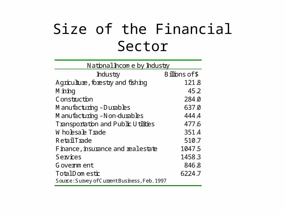
Size of the Financial Sector
National Income by IndustryIndustry Billions of $
Agriculture, forestry and fishing 121.8Mining 45.2Construction 284.0Manufacturing - Durables 637.0Manufacturing - Non-durables 444.4Transportation and Public Utilities 477.6Wholesale Trade 351.4Retail Trade 510.7Finance, insurance and real estate 1047.5Services 1458.3Government 846.8Total Domestic 6224.7Source: Survey of Current Business, Feb. 1997
Transactional Efficiencies
• Phases of Transaction– Search
• Automation efficiencies
• Fewer constraints on search with wider scope
– Negotiation• Online price discovery
– Settlement• Efficiencies associated with electronic clearing of transactions
• Automation and expansion will increase competition among intermediaries, reducing the impact of existing gatekeepers
Value-Added Intermediation
• Transformation functions– Continuing role for intermediaries (such as banks) that allow
transformation of asset structures• Changes in maturity (short-term versus long-term borrowing and lending
activities)
• Volume transformation (aggregation of savings for provision of large loans)
• Information Brokerage– Importance of information in evaluation of risk and uncertainty
– Enhancements on the internet: EDGAR (Electronic Data Gathering, Analysis and Retrieval)
• Online database with all SEC filings and analysis of publicly available information
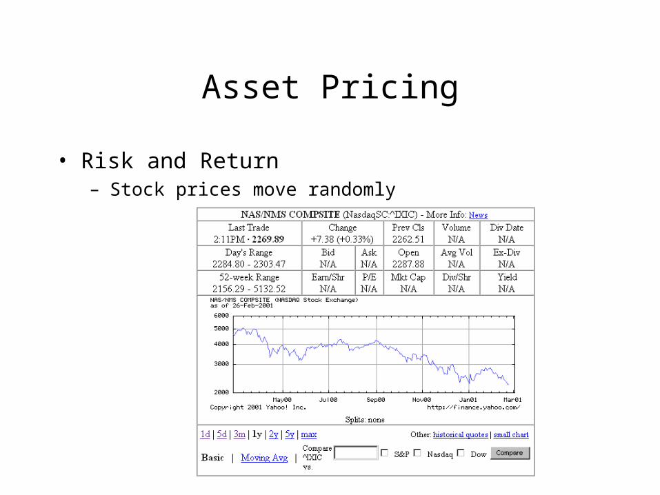
Asset Pricing
• Risk and Return– Stock prices move randomly

Asset Pricing
• Diversification and the law of large number– Model returns as a stochastic process
– N assets, j=1,2,…,N
– Simple model with AR(1) returns:
– Special case with =0: IID returns
10
1,,,0 2
1
ttj
xxj
t
jt
jt
jt

Asset Pricing
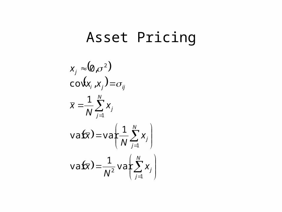
• Construct a portfolio consisting of 1/N shares of each stock– Payoff to the portfolio is the average return
– We measure the risk associated with the portfolio as simply the variance (or standard deviation of the returns).
• Risk of any given asset will be 2
• What is the risk of the average portfolio?
N
j
jt
N
j
jtt N
xN
r11
11

Asset Pricing
NN
N
N
VarN
xN
VarrVar
N
j
N
j
jt
N
j
jtt
2
2
2
1
22
12
1
1
1
1)(
Asset Pricing
• It now follows that for independent random processes, the variance of the average goes to zero as the number of stocks in the portfolio goes to infinity
• Law of Large Numbers
• Result depends critically on the independence assumption– Example with correlated returns
– Extreme case occurs when all returns are identical ex ante as well as ex post
Asset Pricing
N
jj
N
jj
N
jj
ijji
j
xN
x
xN
x
xN
x
xx
x
12
1
1
2
var1
var
1varvar
1
,cov
,0

Asset Pricing
jiij
jiijj
NN
N
x
1
1
and
1
Let
var
,correlated are returns Because
N
1j
22
N
1j
2N
1j

Asset Pricing
• Law of large numbers holds when =0– Independent returns
– Uncorrelated returns
– Hedging portfolios
xN
NNx
NNNN
x
var , as Clearly,
11var
11
var
Then
2
22

CAPM
• Capital Asset Pricing Model– Approximation assumption: returns are roughly normally
distributed

CAPM
• Normal distribution characterized by two parameters: mean and variance (i.e. return and risk)
• Holding different combinations (portfolios) of assets affects the possible combinations of return and risk an investor can obtain
• 2 asset model =proportion of stock 1 held in portfolio– 1-=proportion of stock 2 held in portfolio– Joint distribution of the returns on the two stocks
2
2
,yxy
xyx
y
x
y
x

CAPM
• Return to a portfolio is denoted by z, with
• Average return to the portfolio is
• Variance of the portfolio is
yxz 1
yxEz 1
xyyxzV 121 2222

CAPM
• We can derive the relationship between the mean of the portfolio and its variance by noting that
• Substituting for in the expression for the variance of the portfolio, we find
• To portfolio spreadsheet
yx
yz
2222
2
22 yyxyyxyx yx
yz
yx
yzzV

CAPM
• Multi-asset specification– Choose portfolio which minimizes the variance of the portfolio
subject to generating a specified average return
– Have to perform the optimization since you can no longer solve for the weights from the specification of the relationship between the averages
N
jj
N
jjj xz
1
1
1
where

CAPM
• As with the two asset case, yields a quadratic relationship between average return to the portfolio and its variance, which is called the mean-variance frontier– Frontier indicates possible combinations of risk and return
available to investors when they hold efficient portfolios (i.e. those that minimize the risk associated with getting a specific return
– Optimal portfolio choice can be determined by confronting investor preferences for risk versus return with possibilities

CAPM

CAPM
• Two fund theorem– Introduce possibility of borrowing or lending without risk
– Example: T-bills
– Let rf denote the risk-free rate of return
• Historically, around 1.5%
– The two fund theorem then states that there exists a portfolio of risky assets (which we will denote by S) such that all efficient combinations or risk and return (i.e. those which minimize risk for a given rate of return) can be obtained by putting some fraction of wealth in S while borrowing or lending at the risk-free rate. The portfolio S is called the market portfolio.

CAPM

CAPM
• Implications of the two fund theorem for asset prices– In equilibrium, asset prices will adjust until all portfolios lie on the
security market line

CAPM
• Implications for asset market equilibrium– Risk-averse investors require higher returns to compensate for
bearing increased risk
– Idiosyncratic risk versus market risk
– Equilibrium risk vs. return relationships• Market risk of asset i is defined as the ratio of the covariance between
asset i and the market portfolio to the variance of the market portfolio
2S
iSi

CAPM
• Since iS=iS i S (where iS is the correlation coefficient between asset i and the market portfolio S), we can write
• Finally, since the returns on all assets must be perfectly correlated with those on the market portfolio (in equilibrium), we know that iS=1, so that
S
iiS
S
ii
S
ii

CAPM
• Since the equation for the market line is
it follows that the predicted equilibrium return on a given asset i will be
• The term rS-rf is called the market risk premium since it measures the additional return over the risk-free rate required to get investors to hold the riskier market portfolio.
• Determining rS
• Applications
fSS
f rrrr
fSifi rrrr