on June 26, 2018 Onanewclassof electro...

http://rspa.royDownloaded from

rspa.royalsocietypublishing.org

ResearchCite this article: Bustamante R, RajagopalKR. 2013 On a new class of electro-elasticbodies. II. Boundary value problems. Proc RSoc A 469: 20130106.http://dx.doi.org/10.1098/rspa.2013.0106

Received: 14 February 2013Accepted: 25 March 2013

Subject Areas:mechanics, structural engineering,mathematical modelling

Keywords:implicit constitutive relations,electro-elasticity, boundary value problems,nonlinear elasticity

Author for correspondence:R. Bustamantee-mail: [email protected]

On a new class ofelectro-elastic bodies. II.Boundary value problemsR. Bustamante1 and K. R. Rajagopal2

1Departamento de Ingeniería Mecánica, Universidad de ChileBeaucheff 850, Santiago Centro, Santiago, Chile2Department of Mechanical Engineering, University of Texas A&M,College Station, TX 77843-3123, USA

In part I of this two-part paper, a new theoreticalframework was presented to describe the responseof electro-elastic bodies. The constitutive theory thatwas developed consists of two implicit constitutiverelations: one that relates the stress, stretch and theelectric field, and the other that relates the stress, theelectric field and the electric displacement field. Inpart II, several boundary value problems are studiedwithin the context of such a construct. The governingequations allow for nonlinear coupling between theelectric and stress fields. We consider boundaryvalue problems wherein both homogeneous andinhomogeneous deformations are considered, withthe body subject to an electric field. First, the extensionand the shear of an electro-elastic slab subject to anelectric field are studied. This is followed by a studyof the problem of a thin circular plate and a longcylindrical tube, both subject to an inhomogeneousdeformation and an electric field. In all the boundaryvalue problems considered, the relationships betweenthe stress and the linearized strain are nonlinear, inaddition to the nonlinear relation to the electric field.It is emphasized that the theories that are currentlyavailable are incapable of modelling such nonlinearrelations.

1. IntroductionIn part I of this two-part paper [1], we extended theimplicit constitutive theory proposed by Rajagopal [2–4]for describing the response of elastic bodies that leadto models that are neither Cauchy elastic nor Greenelastic (see Truesdell & Noll [5] for a definition of thesame), to the electro-elastic response of materials. Thisgeneralization involves two sets of implicit constitutive

2013 The Author(s) Published by the Royal Society. All rights reserved.

on September 6, 2018alsocietypublishing.org/

http://crossmark.crossref.org/dialog/?doi=10.1098/rspa.2013.0106&domain=pdf&date_stamp=2013-04-24

mailto:[email protected]

http://rspa.royalsocietypublishing.org/

2

rspa.royalsocietypublishing.orgProcRSocA469:20130106

..................................................

on September 6, 2018http://rspa.royalsocietypublishing.org/Downloaded from

relations, one between the stress, the Cauchy–Green tensor and the electric field and an implicitrelation between the stress, the electric field and the electric displacement field. The theorydeveloped was also restricted to a simplified form of Maxwell’s equations. Unlike the studiesof Rajagopal & Srinivasa [6,7] that consider implicit constitutive relations for elastic bodieswithin the context of a thermodynamic framework, our generalization to electro-elasticity wasnot within the context of a fully thermodynamic framework but was restricted to mechanical,electrical and magnetic effects. After developing implicit constitutive relations that are capable ofdescribing large deformations, we obtained approximations wherein the displacement gradientand the electric displacement are assumed to be small; the constitutive relations, however, yetbeing nonlinear. As discussed in part I, such constitutive relations are capable of describing thenonlinear response that is observed in piezoelectric bodies, which the classical small displacementgradient theories are incapable of describing.

A special subclass of the fully implicit constitutive relations is one wherein explicit constitutiverelations are prescribed for the Cauchy–Green stretch in terms of the stress, the electric field andthe electric displacement vector. This constitutive relation can also be approximated by assumingthat the displacement gradient and the electric displacement vector are appropriately small. Thispart of the paper is devoted to the study of boundary value problems corresponding to bothhomogeneous and inhomogeneous states of stress, within the context of such an approximation.We first consider the homogeneous state of stress of a slab, first when subject to traction, andthen when subject to shear, the slab being in the presence of an electric field in both problems.This is followed by the analysis of a thin circular plate which is inflated in the radial direction,wherein the state of stress is inhomogeneous. Finally, we study the inhomogeneous inflation ofa long cylindrical annulus. In all the boundary value problems that were studied, the strainsremain very small, though the stresses and the electrical field are large, and, more importantly,the relationship between the stress and the linearized strain is nonlinear. We cannot emphasizeenough the fact that unlike the present theory, the theories that are currently in place are incapableof describing a nonlinear relationship between the linearized strain and the stress.

2. Basic equations

(a) Kinematics and the equations of electrostaticsLet X ∈ κR(B) denote a particle belonging to a body B in the reference configuration κR(B), and letx ∈ κt(B) denote the position of the same particle in the current configuration κt(B), at time t. Weshall assume that the mapping χ , which assigns the position x at time t, x = χ(X, t) is sufficientlysmooth so as to make all the derivatives that are taken, meaningful. The displacement u, thedeformation gradient F, the Cauchy–Green stretch tensors b and c and the linearized strain ε aredefined through

u = x − X, F = ∂χ

∂X, b = FFT, c = FTF, ε = 1

2

[(∂u∂x

)+(

∂u∂x

)T]

. (2.1)

More details concerning kinematics can be found in references [8,9]. In this paper, we areinterested in studying quasi-static problems of electro-elastic bodies.

We denote by E and D, respectively, the electric field and the electric displacement in thecurrent configuration. The fields E and D satisfy a simplified form of Maxwell’s equations inthe absence of magnetic interactions, distributed charges and time dependence, namely

curl E = 0, div D = 0. (2.2)

In vacuum B′, the following relation is valid:

D = ε0E, (2.3)

where ε0 is the electric permittivity in vacuum.


3


..................................................


The polarization field P for condensed matter is defined as

P = D − ε0E. (2.4)

Across a surface of discontinuity in the body or the boundary ∂κt(B), considering there is nodistribution of electric surface charges, the fields E and D have to satisfy the continuity conditions

n × [[E]] = 0, n · [[D]] = 0, (2.5)

where n is the unit outward normal to ∂κt(B). The double brackets represent the jump acrossthe surface of discontinuity, for example, [[D]] = Do − Di, where Do and Di would be the electricdisplacements on either side of the boundary, respectively (evaluated very close to the surface ofdiscontinuity). More detail about the theory of electromagnetism can be found, for example, inKovetz [10].

There are different ways in which the equilibrium equations can be used when dealing withelectromagnetic interactions [11]. A simple formulation is based on the use of a ‘total stress’ tensorτ , which incorporates in its definition a term related with the electric body forces [12]. This totalstress tensor is symmetric and in the current configuration the equilibrium equation is of the form(in the absence of time dependence)

div τ + ρf = 0. (2.6)

The continuity condition across a surface of discontinuity of the surface of the body ∂κt(B) inthe current configuration is of the form [12,13]

[[τ ]]n = 0, (2.7)

where if ta is the mechanical traction per unit area, then the above condition implies that

τn = ta + τmn, (2.8)

where τm is the Maxwell stress due to the electric field outside the material near the boundary ofthe body [11]

τm = Do ⊗ Eo − 12 (Do · Eo)I. (2.9)

(b) Some new constitutive relations for electro-elastic bodiesWe [1] proposed the following implicit relations to describe the response of electro-elastic bodies:

f(τ , b, E) = 0, l(τ , E, D) = 0, (2.10)

where f is a tensor implicit relation and l is a vector implicit relation. In this paper, we work withthe subclass of (2.10), which is a consequence of a linearization based on ‖∇u‖∼ O(δ), δ � 1. Weconsider the special subclass that takes the form

ε = f(τ , E), l(τ , E, D) = 0. (2.11)

For isotropic functions f and l, (2.11) leads to (see §3.3 of Bustamante & Rajagopal [1])

ε = α0I + α1τ + α2τ2 + α3E ⊗ E + α4(E ⊗ τE + τE ⊗ E) + α5(E ⊗ τ 2E + τ 2E ⊗ E) (2.12)

and

β0E + β1τE + β2τ2E + β3D + β4τD + β5τ

2D + β6[τ (E × D) + (τD) × E)] = 0, (2.13)

where αi, i = 0, . . . , 5 are scalar functions that depends on the invariants (see Spencer [14])

I1 = tr τ , I2 = tr τ 2, I3 = tr τ 3, I4 = E · E, I5 = E · (τE), I6 = E · (τ 2E) (2.14)


4


..................................................


and βj, j = 0, 1, . . . , 6 are scalar functions that depend on the invariants (2.14) and the invariants

I7 = D · D, I8 = D · (τD), I9 = D · (τ 2D), I10 = (D · E)2, I11 = [D · (τE)]2. (2.15)

We shall also consider the approximation to (2.10) under the assumptions ‖∇u‖∼ O(δ) and‖D‖∼ O(δ) with δ � 1; in fact, we shall consider the special subclass of electro-elastic bodiesdefined by

ε = f(τ , E), D = l(τ , E). (2.16)

For isotropic functions f and l, (2.16)1 reduces to (2.12), whereas (2.16)2 leads to

D = β0E + β1τE + β2τ2E. (2.17)

The functions βj, j = 0, 1, 2 depend on the invariants (2.14).In what follows, we solve some boundary value problems that are governed by

equations (2.12), (2.13) and (2.12), (2.17) in order to determine the efficacy of such models. Wefirst consider problems wherein the stress and the electrical field are homogeneous and weconsider problems within the confines of the constitutive relations (2.12) and (2.13). We followthis with a study of a problem wherein the stress and the electrical field within the body areinhomogeneous, within the context of constitutive equations (2.12) and (2.17), where we assumethat the functions f and l are isotropic, although in many applications involving electro-activebodies, it is necessary to work with anisotropic bodies. As outlined in part I, applications suchas piezoelectricity demand the use of such anisotropic bodies. However, there is a dearth ofexperimental data against which one can corroborate the predictions of the theory, especiallyin reasonably simple geometries wherein one can solve initial boundary value problems, as theequations are nonlinear and quite complicated. Moreover, it is important to first solve problemsin simple enough geometries to assess the usefulness of such models before embarking on studiesof boundary value problems in complicated geometries.

(c) Boundary value problemsWe shall first give a short account of some important issues concerning the solution of boundaryvalue problems within the context of nonlinear electro-elasticity. Unlike classical problems inelasticity (or electro-elasticity), wherein the expression for the stress is substituted into the balanceof linear momentum that leads to an equation for the displacement field (and the electric field),we now have the situation wherein the constitutive relation has to be solved simultaneouslywith the balance of linear momentum. Thus, the stress is also a primitive in this approach. Thebasic variables that we work with are: the total stress tensor τ , the electric field E, the electricdisplacement D, the linearized strain tensor ε and the displacement field u. These quantities haveto satisfy the implicit constitutive relations (2.11): ε = f(τ , E), l(τ , E, D) = 0 (or (2.16)2 D = l(τ , E)),the equilibrium equation (no mechanical body forces and time dependence) (2.6): div τ = 0, thesimplified form of the Maxwell equations (2.2) (considering no time dependence): curl E = 0,div D = 0 and the kinematical relation (2.1)5, namely ε = 1

2 [∇u + (∇u)T].Let us assume that the electric field is expressed through a scalar electric potential ϕ in the

following manner:

E = −grad ϕ. (2.18)

Such a potential would automatically satisfy (2.2)1. To summarize, we need to find ε, τ , ϕ, D bysolving the equations (2.11), (2.6), (2.2)2 and (2.1)5

ε = f(τ , E), l(τ , E, D) = 0, div τ = 0, div D = 0, ε = 12 [∇u + (∇u)T], (2.19)

and considering (2.16)2 instead of (2.11)2 in the case ‖D‖∼ O(δ) with δ � 1.


5


..................................................


There are six components each for the strain and total stress tensors, three components forthe electric displacement and the displacement field, and one component for the electric scalarpotential; therefore there are 19 unknowns. If we count the number of equations in (2.19), thenthere are six equations from f, three for l (or l in the case of (2.16)2), three equilibrium equationsfor the stress, one equation for the electric displacement and six for the strain–displacementkinematics relation; therefore we have in total 19 equations, and so the problem is determinate.

An alternative method to solve the boundary value problem is to introduce a stress tensorpotential, where (see equation (227.10) in §227 of Truesdell & Toupin [9])

τ km = ekrpemsqars,pq, (2.20)

where ekrp is the permutation symbol and ars = asr are the components of the stress tensorpotential. In such a case, (2.19)3 would be satisfied automatically. If we assume again that (2.18)holds, then we would need to find the six components of ars, the six components of ε, the threecomponents of D and the scalar electric potential ϕ; therefore, in this alternative case, we wouldneed to find 16 unknowns. These unknowns should be found by solving (2.19)1 (six equations),(2.19)2 (three equations), (2.19)4 (one equation) and (2.19)5 would be replaced by the compatibilityequations (only six are independent) [9]:

R(ε)

kmpq = 0, (2.21)

where the components of the Riemann tensor R(ε)

kmpq are defined in terms of ε, for example inequation (34.2) of Truesdell & Toupin [9] (the compatibility equations are necessary in order toobtain a unique displacement field solving (2.19)5); therefore, we have, in total, 16 unknowns andagain the problem is determinate.

If we are interested in solving the boundary value problem without using (2.18), we wouldhave to consider the 19 equations in (2.19) plus (2.2)1, which has three components, so in total wewould have 22 equations to be solved. However, with regard to the unknowns, we would havethe 18 independent components of ε, τ , D and u, plus the three components of E, so in total thereare 21 unknowns, which would make the problem ill-conditioned (unless we use (2.18)). This is aninteresting fact about the simplified form of the Maxwell equations used in this work; we wouldnot run into such a difficulty when using the full system of Maxwell’s equations and the balanceof linear momentum; for a detailed discussion, see [15] in particular §3 therein.

With regard to the boundary conditions, in most of the works published in electro-elasticity,the investigators have considered only the body and not the surrounding space for the analysis,but Maxwell’s equations (and its specializations (2.2)) have to be satisfied not only for the electro-elastic body under consideration, but also for the whole surrounding space (see the discussion inKovetz [10]). It is important to recognize this aspect to the problem in order to obtain a meaningfulsolution; however, if one is only interested in the response of the electro-elastic body, we enforcethe usual boundary conditions for the displacement field and the stress

u = u(x) x ∈ ∂κut (B), τn = t(x) x ∈ ∂κ t

t (B),

and for the electric variables (assuming ϕ is the basic variable, in virtue of its clear physicalmeaning in electrostatics [10,16]):

ϕ = ϕ(x) x ∈ ∂κϕt (B), D · n = D(x) · n x ∈ ∂κD

t (B),

where u, t, ϕ and D are known fields on the boundary of the body in the current configurationκt(B), where ∂κt(B) = ∂κu

t (B) ∪ ∂κ tt (B) = ∂κ

ϕt (B) ∪ ∂κu

D(B), and ∂κut (B) ∩ ∂κ t

t (B) = Ø, ∂κϕt (B) ∩

∂κDt (B) = Ø. If we assume for simplicity that the body is in free vacuum, it is possible to show

that the presence of the surrounding space could have an important impact on the distribution ofelectric field, and therefore in the deformation of the body, because of the continuity conditions(2.5), (2.7) (for the equivalent magnetoelastic problem see [17,18]). The effect of considering theexterior free space depends on the geometry of the body, and in particular on its electromechanicalbehaviour and the magnitude of the electric susceptibility in vacuum ε0 [19].


6


..................................................


We make two additional remarks before turning our attention to presenting solutions to somesimple boundary value problems:

— the fulfillment of the continuity conditions (2.5) for ‘finite’ geometries is not easy toachieve. In the classical theory of nonlinear electro-elasticity, there is one exact solution,to the best of our knowledge, for a boundary value problem that takes into account (2.5)for electro-active bodies of finite size; almost all exact solutions that have been establishedthus far have been obtained assuming infinite long tubes, slabs and cylinders (see [20]),the only exception being the problem of inflation of a sphere, see §5 of [13];

— regarding the boundary conditions for the traction, we must recognize that mechanicalsurface traction can be applied only by the interaction with the surface of another externalbody (see the discussion in Bustamante [21]). In the case of the traction associated withMaxwell stresses that appears in (2.8) (see (2.9)), for the sake of simplicity, we will assumethat such Maxwell stresses can be incorporated into the definition of the external traction(see the discussion in McMeeking & Landis [22]); and

— when the bodies are in empty space, we consider the Maxwell stresses (2.9) as externaltraction loads in (2.8) [23].

3. Homogeneous stresses and electrical fieldLet us consider two simple problems wherein we can assume that we have a homogeneousdistribution of the total stress and the electric field.

(a) Slab under tractionLet us consider a slab defined through

− L1

2≤ x1 ≤ L1

2− L2

2≤ x2 ≤ L2

2, −L3

2≤ x3 ≤ L3

2. (3.1)

Because we work under the assumption of small gradient for the displacement field, we donot make a distinction between the current and the reference configurations; therefore, in thisparticular problem and in the three problems that are described later, the body is described byusing the coordinates in the current configuration.

Let us assume that L3 � L1 and L2 � L1. Let us further assume that the stress and the electricfield are of the form:1

τ =3∑

i=1

τ0i ei ⊗ ei, E = E0e1, (3.2)

where τ0i , i = 1, 2, 3 and E0 are constants; therefore (2.19)3 and (2.2)1 are automatically satisfied. Inthis case, it follows from (2.12) that

ε11 = α0 + α1τ01 + α2τ201

+ α3E20 + 2α4E2

0τ01 + 2α5E20τ

201

(3.3)

and

ε22 = α0 + α1τ02 + α2τ202

, ε33 = α0 + α1τ03 + α2τ203

, (3.4)

and εij = 0, i = j, i, j = 1, 2, 3. The scalar functions αq, q = 0, 1, . . . , 5 depend on the invariants (2.14)

I1 = τ01 + τ02 + τ03 , I2 = τ 201

+ τ 202

+ τ 203

, I3 = τ 301

+ τ 302

+ τ 303

(3.5)

and

I4 = E20, I5 = E2

0τ01 , I6 = E20τ

201

. (3.6)

1For problems where we consider uniform distribution of electric field, it is not necessary to use (2.18) because (2.2)1 issatisfied trivially.


7


..................................................


Because τ0i , i = 1, 2, 3 are constant, and because in virtue of (3.3)–(3.6), we can also conclude thatthe components of the strain are constant, it follows that the compatibility equations (2.21) aresatisfied and from (2.19)5 a unique u can be calculated.

From (3.2) and (2.13), it cannot be said immediately that D has only a component in the x1-direction; therefore, we shall assume that in general D is of the form

D = Diei. (3.7)

From (3.2) and (2.13), we obtain that

β0E0 + β1τ01 E0 + β2τ201

E0 + β3D1 + β4τ01 D1 + β5τ201

D1 = 0, (3.8)

(β3 + β4τ02 + β5τ202

)D2 + β6τ02 E0D3 = 0 (3.9)

and β6(τ03 − τ02)E0D2 + (β3 + β4τ03 + β5τ203

)D3 = 0, (3.10)

where the functions βr, r = 0, 1, 2, . . . , 6 depend on the invariants (3.5) and (3.6) and the invariants(2.15)

I7 = D21, I8 = D2

1τ01 , I9 = D21τ

201

, I10 = D21E2

0, I11 = D21τ

201

E20. (3.11)

We note that (3.9) and (3.10) can be written as(β3 + β4τ02 + β5τ

202

β6τ02 E0

β6(τ03 − τ02 )E0 β3 + β4τ03 + β5τ203

)(D2D3

)=(

00

). (3.12)

If M denotes the matrix M=(

β3+β4τ02 +β5τ202

β6τ02 E0

β6(τ03 −τ02 )E0 β3+β4τ03 +β5τ203

), we have two possible solutions for D.

One solution is obtained if we assume D2 = D3 = 0, but there could be another possibility, whichis to assume that in general D2 = 0 and D3 = 0, and detM= 0. In that case, it follows from (3.11)that equation detM= 0 would be, in general, a nonlinear relation for D1. If D1 is found such thatboth detM= 0 and (3.8) are satisfied, then from (3.12) there would be other possibilities for D2 andD3 and one of the two would be arbitrary.

For the sake of simplicity, let us consider the solution D2 = D3 = 0, then from (3.5), (3.6), (3.11)and (3.8), we would have an algebraic equation (in general nonlinear) to obtain D1 in terms of E0and τ0i , i = 1, 2, 3. Because such a value for D1 would be constant, then (2.19)4 would be satisfiedautomatically.

We thus have a solution for the set of equations (2.19); let us now turn our attention to adiscussion of the boundary conditions. At the surfaces x1 = ±L1/2, if we want (2.5)2 to be satisfied,then we need

Do1 = D1, (3.13)

where Do1 is the electric displacement outside the body at the boundary. From (2.3), for vacuum

we would have

Do1 = ε0Eo

1. (3.14)

Across the surfaces x2 = ±L2/2 and x3 = ±L3/2 in order for the continuity condition (2.5)1 tobe satisfied we would need Eo

1 = E0, but this condition in general does not give the same valuefor Eo

1 as that which is obtained from (3.13) to (3.14); however, if L3 � L1 and L2 � L1, the surfacesx2 = ±L2/2 and x3 = ±L3/2 are located far away, and so, as an approximation, we do not considerthe electric continuity conditions for such surfaces.

Therefore, from the point of view of the electric field, from the exterior space we need (as anapproximation) an electric field of the form

E = Eo1e1, (3.15)

where Eo1 is obtained from (3.14) and (3.13). Such an electric field and the electric displacement

associated with it are constant and so they satisfy the simplified forms of Maxwell equations forvacuum.


8


..................................................


With regard to the mechanical boundary conditions, we assume that at the surfaces x2 = ±L2/2and x3 = ±L3/2 external mechanical forces are applied such that the total stress inside the body isgiven by (3.2)1. If we denote t to be this external mechanical traction, from τn = t we find that onthe surfaces x2 ± L2/2 and x3 ± L3/2

t = ±τ02 e2, t = ±τ03 e2, (3.16)

respectively. As for the surface x1 = ±L1/2, we assume that the body is exposed to free vacuum,and the traction will be found using the Maxwell stress (2.9). Using (3.15) and (2.3) for the exteriorfield, from (2.9) we have

τm = ε0(Eo1)2

2(e1 ⊗ e1 − e2 ⊗ e2 − e3 ⊗ e3), (3.17)

and so from (3.17) we find that τmn = (ε0(Eo1)2/2)e1 on the surface x1 = L1/2 and τmn =

−(ε0(Eo1)2/2)e1 on the surface x1 = −L1/2; therefore, from (2.8) we have

τ01 = ε0(Eo1)2

2on x1 = ±L1/2. (3.18)

We note that in (3.2)1 the stress τ01 is not an arbitrary quantity, but depends on the magnitude ofthe electric field.

(b) A slab in a state of shearFor the problem in question, we shall assume a solution for stress and electric field of the form

τ = τ012(e1 ⊗ e2 + e2 ⊗ e1), E = E0e1, (3.19)

where τ012 and E0 are constant. We consider the same geometry defined by (3.1), but for thisproblem, we assume that the external force is applied at the surfaces x1 = ±L1/2. From (2.12), weobtain that

ε11 = α0 + α1τ2012

+ α3E20 + α5τ

2012

E20, ε22 = α0 + α2τ

2012

, ε33 = α0 (3.20)

and

ε12 = α1τ012 + α4τ012 E20, ε13 = ε23 = 0, (3.21)

whereas from (2.13), we have

β0E0 + β2τ2012

E0β3D1 + β4τ012 D2 + β5τ2012

D1 − β6E0D3τ012 = 0, (3.22)

β1τ012 E0 + β3D2 + β4τ012 D1 + β5τ2012

D2 = 0 (3.23)

and β3D3 − β6E0τ012 D1 = 0, (3.24)

where Ii, i = 1, 2, . . . , 11 are given from (2.14), (2.15)

I1 = I3 = I5 = 0, I2 = 2τ 2012

, I4 = E20, I6 = τ 2

012E2

0, I7 = D21 + D2

2 + D23 (3.25)

and

I8 = 2τ012 D1D2, I9 = τ 2012

(D21 + D2

2), I10 = D21E2

0, I11 = τ 2012

E20D2

2. (3.26)

From (3.23) and (3.24), in general, D2 and D3 are different from zero, unlike the previous problemstudied in §3a.

Regarding the continuity conditions (2.7), the assumption is that the mechanical traction isapplied at the surfaces x1 = ±L1/2. For these surfaces, on using (2.5)2, we find that D1 = Do

1 andso from (2.3), we obtain Eo

1 = ε−10 Do

1 = ε−10 D1. Regarding (2.5)2, from (3.19), we obtain Eo

2 = Eo3 = 0

at x1 = ±L1/2. Because L1 � L2 and L1 � L3, the surfaces x2 = ±L2/2 and x3 = ±L3/2 are far away,and thus we do not check the continuity conditions (2.5) at those surfaces.


9


..................................................


4. Non-homogeneous distribution of stressesIn this section, for the sake of simplicity, only the constitutive relations given by (2.16) will beconsidered, which in the case of isotropic functions f, l reduce to (2.12) and (2.17). For the classof problem discussed here, complex ordinary differential equations will be obtained, which aresolved using numerical methods; therefore, some additional assumptions are needed regardingthe constitutive equations (2.16) in order to obtain closed form solutions.

We assume there exists a scalar function Ω = Ω(τ , E) such that

ε = ∂Ω

∂τ, D = −∂Ω

∂E. (4.1)

This assumption has been made with the purpose of facilitating the development ofprototypical expressions for the functions αi and βj, i = 0, 1, . . . , 5 and j = 0, 1, 2 in (2.11) and (2.17).The function Ω has not been obtained on the basis of thermodynamic arguments; such an analysisis beyond the scope of this work.

For an isotropic function Ω = Ω(I1, I2, I3, I4, I5, I6), where Ik, k = 1, 2, . . . , 6 are defined in (2.14).Using the chain rule for the derivative (in index notation for a Cartesian coordinate system) from(4.1), we have εij = ∂Ω/∂τij =∑6

k=1(∂Ω/∂Ik)(∂Ik/∂τij) and Di = −∑6k=1(∂Ω/∂Ik)(∂Ik/∂Ei), which

after some algebraic manipulations become

ε = ∂Ω

∂I1I + 2

∂Ω

∂I2τ + 3

∂Ω

∂I3τ 2 + ∂Ω

∂I5E ⊗ E + ∂Ω

∂I6(E ⊗ τE + τE ⊗ E) (4.2)

and

D = −2(

∂Ω

∂I4E + ∂Ω

∂I5τE + ∂Ω

∂I6τ 2E

), (4.3)

with the following relationships holding:

α0 = ∂Ω

∂I1, α1 = 2

∂Ω

∂I2, α2 = 3

∂Ω

∂I3, α3 = ∂Ω

∂I5, α4 = ∂Ω

∂I6, α5 = 0 (4.4)

and

β0 = −2∂Ω

∂I4, β1 = −2

∂Ω

∂I5, β2 = −2

∂Ω

∂I6. (4.5)

We shall consider the resolution of boundary value problems in electro-elasticity, wherein theclass of bodies of interest exhibit two characteristics: the first is the strain limiting behaviour thatis exhibited by a large class of electro-elastic bodies, the second is the saturation phenomenon forthe polarization field P in terms of the intensity of the electric field. Thus, it is imperative that onepicks constitutive relations that reflect such characteristics.

In Bustamante & Rajagopal [24] (see also Ortiz et al. [25]), a scalar function Ω was proposedso that the model exhibits ‘strain-limiting’ behaviour; the specific form chosen for Ω is −α[I1 −(1/β) ln(1 + βI1)] + (αγ /ι)

√1 + ιI2, where α, β, γ and ι are constants. An interesting feature of

such a function is that it is not only strain limiting but the model also exhibits different responsewith regard to compression and tension. From the point of view of numerical computations,some difficulties arise when I1 < 0, especially when βI1 → −1; therefore, a modified version ofthe function presented in Bustamante & Rajagopal [24] is used here, that is Ω is of the form−α[I1 − ∫I1

0 (1/(1 + β(� 2)b)) d� ] + (αγ /ι)√

1 + ιI2, where b is a constant with b > 12 .

In Bustamante [26], an expression for an energy function was proposed for the equivalentmagnetoelastic problem, which produces the saturation phenomena (in that case for themagnetization) discussed within the context of fig. 1 in Bustamante & Rajagopal [1], such afunction has the form (for isotropic bodies): (elastic part)(g0 + g1I4) − ln[cosh(

√I4/m1)]m0m1 −

(ζ0/2)I4 + (ε0ζ1/2)I5, where g0, g1, m0, m1, ζ0 and ζ1 are constants.


10


..................................................


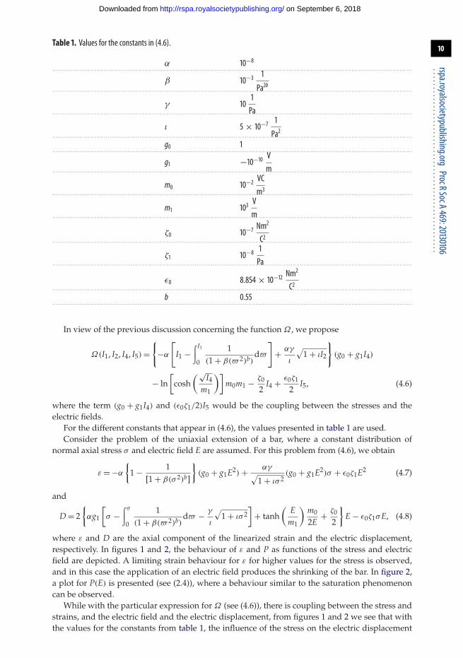
Table 1. Values for the constants in (4.6).

α 10−8. . . . . . . . . . . . . . . . . . . . . . . . . . . . . . . . . . . . . . . . . . . . . . . . . . . . . . . . . . . . . . . . . . . . . . . . . . . . . . . . . . . . . . . . . . . . . . . . . . . . . . . . . . . . . . . . . . . . . . . . . . . . . . . . . . . . . . . . . . . . . . . . . . . . . . . . . . . . . . . . . . . . . . . . . . . . . . . . . . . . . . . . . . . . . . . . . . . . . . . . . .

β 10−3 1

Pa2b. . . . . . . . . . . . . . . . . . . . . . . . . . . . . . . . . . . . . . . . . . . . . . . . . . . . . . . . . . . . . . . . . . . . . . . . . . . . . . . . . . . . . . . . . . . . . . . . . . . . . . . . . . . . . . . . . . . . . . . . . . . . . . . . . . . . . . . . . . . . . . . . . . . . . . . . . . . . . . . . . . . . . . . . . . . . . . . . . . . . . . . . . . . . . . . . . . . . . . . . . .

γ 101Pa. . . . . . . . . . . . . . . . . . . . . . . . . . . . . . . . . . . . . . . . . . . . . . . . . . . . . . . . . . . . . . . . . . . . . . . . . . . . . . . . . . . . . . . . . . . . . . . . . . . . . . . . . . . . . . . . . . . . . . . . . . . . . . . . . . . . . . . . . . . . . . . . . . . . . . . . . . . . . . . . . . . . . . . . . . . . . . . . . . . . . . . . . . . . . . . . . . . . . . . . . .

ι 5 × 10−7 1

Pa2. . . . . . . . . . . . . . . . . . . . . . . . . . . . . . . . . . . . . . . . . . . . . . . . . . . . . . . . . . . . . . . . . . . . . . . . . . . . . . . . . . . . . . . . . . . . . . . . . . . . . . . . . . . . . . . . . . . . . . . . . . . . . . . . . . . . . . . . . . . . . . . . . . . . . . . . . . . . . . . . . . . . . . . . . . . . . . . . . . . . . . . . . . . . . . . . . . . . . . . . . .

g0 1. . . . . . . . . . . . . . . . . . . . . . . . . . . . . . . . . . . . . . . . . . . . . . . . . . . . . . . . . . . . . . . . . . . . . . . . . . . . . . . . . . . . . . . . . . . . . . . . . . . . . . . . . . . . . . . . . . . . . . . . . . . . . . . . . . . . . . . . . . . . . . . . . . . . . . . . . . . . . . . . . . . . . . . . . . . . . . . . . . . . . . . . . . . . . . . . . . . . . . . . . .

g1 −10−10 Vm. . . . . . . . . . . . . . . . . . . . . . . . . . . . . . . . . . . . . . . . . . . . . . . . . . . . . . . . . . . . . . . . . . . . . . . . . . . . . . . . . . . . . . . . . . . . . . . . . . . . . . . . . . . . . . . . . . . . . . . . . . . . . . . . . . . . . . . . . . . . . . . . . . . . . . . . . . . . . . . . . . . . . . . . . . . . . . . . . . . . . . . . . . . . . . . . . . . . . . . . . .

m0 10−2 VCm3

. . . . . . . . . . . . . . . . . . . . . . . . . . . . . . . . . . . . . . . . . . . . . . . . . . . . . . . . . . . . . . . . . . . . . . . . . . . . . . . . . . . . . . . . . . . . . . . . . . . . . . . . . . . . . . . . . . . . . . . . . . . . . . . . . . . . . . . . . . . . . . . . . . . . . . . . . . . . . . . . . . . . . . . . . . . . . . . . . . . . . . . . . . . . . . . . . . . . . . . . . .

m1 103Vm. . . . . . . . . . . . . . . . . . . . . . . . . . . . . . . . . . . . . . . . . . . . . . . . . . . . . . . . . . . . . . . . . . . . . . . . . . . . . . . . . . . . . . . . . . . . . . . . . . . . . . . . . . . . . . . . . . . . . . . . . . . . . . . . . . . . . . . . . . . . . . . . . . . . . . . . . . . . . . . . . . . . . . . . . . . . . . . . . . . . . . . . . . . . . . . . . . . . . . . . . .

ζ0 10−7 Nm2

C2. . . . . . . . . . . . . . . . . . . . . . . . . . . . . . . . . . . . . . . . . . . . . . . . . . . . . . . . . . . . . . . . . . . . . . . . . . . . . . . . . . . . . . . . . . . . . . . . . . . . . . . . . . . . . . . . . . . . . . . . . . . . . . . . . . . . . . . . . . . . . . . . . . . . . . . . . . . . . . . . . . . . . . . . . . . . . . . . . . . . . . . . . . . . . . . . . . . . . . . . . .

ζ1 10−8 1Pa. . . . . . . . . . . . . . . . . . . . . . . . . . . . . . . . . . . . . . . . . . . . . . . . . . . . . . . . . . . . . . . . . . . . . . . . . . . . . . . . . . . . . . . . . . . . . . . . . . . . . . . . . . . . . . . . . . . . . . . . . . . . . . . . . . . . . . . . . . . . . . . . . . . . . . . . . . . . . . . . . . . . . . . . . . . . . . . . . . . . . . . . . . . . . . . . . . . . . . . . . .

ε0 8.854 × 10−12 Nm2

C2. . . . . . . . . . . . . . . . . . . . . . . . . . . . . . . . . . . . . . . . . . . . . . . . . . . . . . . . . . . . . . . . . . . . . . . . . . . . . . . . . . . . . . . . . . . . . . . . . . . . . . . . . . . . . . . . . . . . . . . . . . . . . . . . . . . . . . . . . . . . . . . . . . . . . . . . . . . . . . . . . . . . . . . . . . . . . . . . . . . . . . . . . . . . . . . . . . . . . . . . . .

b 0.55. . . . . . . . . . . . . . . . . . . . . . . . . . . . . . . . . . . . . . . . . . . . . . . . . . . . . . . . . . . . . . . . . . . . . . . . . . . . . . . . . . . . . . . . . . . . . . . . . . . . . . . . . . . . . . . . . . . . . . . . . . . . . . . . . . . . . . . . . . . . . . . . . . . . . . . . . . . . . . . . . . . . . . . . . . . . . . . . . . . . . . . . . . . . . . . . . . . . . . . . . .

In view of the previous discussion concerning the function Ω , we propose

Ω(I1, I2, I4, I5) ={

−α

[I1 −

∫ I1

0

1(1 + β(� 2)b)

d�

]+ αγ

ι

√1 + ιI2

}(g0 + g1I4)

− ln[

cosh(√

I4

m1

)]m0m1 − ζ0

2I4 + ε0ζ1

2I5, (4.6)

where the term (g0 + g1I4) and (ε0ζ1/2)I5 would be the coupling between the stresses and theelectric fields.

For the different constants that appear in (4.6), the values presented in table 1 are used.Consider the problem of the uniaxial extension of a bar, where a constant distribution of

normal axial stress σ and electric field E are assumed. For this problem from (4.6), we obtain

ε = −α

{1 − 1

[1 + β(σ 2)b]

}(g0 + g1E2) + αγ√

1 + ισ 2(g0 + g1E2)σ + ε0ζ1E2 (4.7)

and

D = 2{αg1

[σ −

∫ σ

0

1(1 + β(� 2)b)

d� − γ

ι

√1 + ισ 2

]+ tanh

(E

m1

)m0

2E+ ζ0

2

}E − ε0ζ1σE, (4.8)

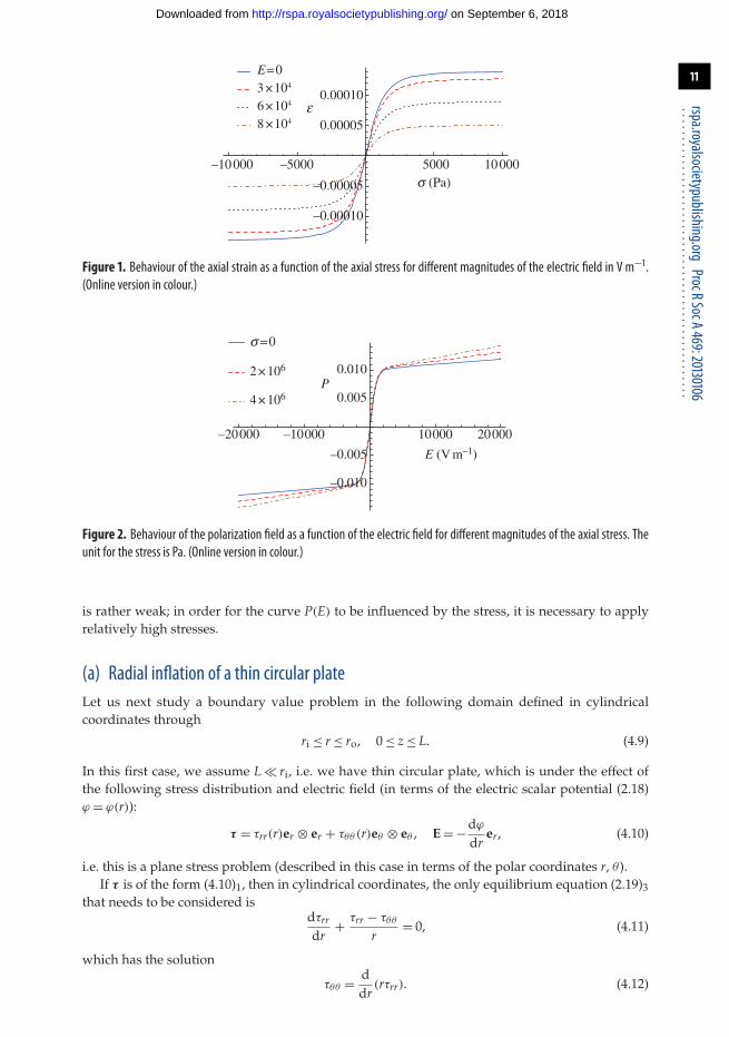
where ε and D are the axial component of the linearized strain and the electric displacement,respectively. In figures 1 and 2, the behaviour of ε and P as functions of the stress and electricfield are depicted. A limiting strain behaviour for ε for higher values for the stress is observed,and in this case the application of an electric field produces the shrinking of the bar. In figure 2,a plot for P(E) is presented (see (2.4)), where a behaviour similar to the saturation phenomenoncan be observed.

While with the particular expression for Ω (see (4.6)), there is coupling between the stress andstrains, and the electric field and the electric displacement, from figures 1 and 2 we see that withthe values for the constants from table 1, the influence of the stress on the electric displacement


11


..................................................


–10000 –5000 5000 10000

–0.00010

–0.00005

0.00005

0.00010

s (Pa)

e

E=03×104

6×104

8×104

Figure 1. Behaviour of the axial strain as a function of the axial stress for different magnitudes of the electric field in V m−1.(Online version in colour.)

–20000 20000–10000 10000

–0.010

–0.005

0.005

0.010

E (V m–1)

P

s =0

2×106

4×106

Figure 2. Behaviour of the polarization field as a function of the electric field for different magnitudes of the axial stress. Theunit for the stress is Pa. (Online version in colour.)

is rather weak; in order for the curve P(E) to be influenced by the stress, it is necessary to applyrelatively high stresses.

(a) Radial inflation of a thin circular plateLet us next study a boundary value problem in the following domain defined in cylindricalcoordinates through

ri ≤ r ≤ ro, 0 ≤ z ≤ L. (4.9)

In this first case, we assume L � ri, i.e. we have thin circular plate, which is under the effect ofthe following stress distribution and electric field (in terms of the electric scalar potential (2.18)ϕ = ϕ(r)):

τ = τrr(r)er ⊗ er + τθθ (r)eθ ⊗ eθ , E = −dϕ

drer, (4.10)

i.e. this is a plane stress problem (described in this case in terms of the polar coordinates r, θ ).If τ is of the form (4.10)1, then in cylindrical coordinates, the only equilibrium equation (2.19)3

that needs to be considered isdτrr

dr+ τrr − τθθ

r= 0, (4.11)

which has the solution

τθθ = ddr

(rτrr). (4.12)


12


..................................................


On using (4.6) in (4.2) by appealing to (4.10), we obtain

εrr = −α

{1 − 1

[1 + β(I21)

b]

}(g0 + g1I4) + αγ√

1 + ιI2(g0 + g1I4)τrr + ε0ζ1E2

r , (4.13)

εθθ = −α

{1 − 1

[1 + β(I21)

b]

}(g0 + g1I4) + αγ√

1 + ιI2(g0 + g1I4)τθθ (4.14)

and εzz = −α

{1 − 1

[1 + β(I21)

b]

}(g0 + g1I4), (4.15)

where

I1 = τrr + ddr

(rτrr), I2 = τ 2rr +

[ddr

(rτrr)

]2, I4 =

(dϕ

dr

)2. (4.16)

In order for the strain components (4.13)–(4.15) to have an associated continuous displacementfield, certain compatibility conditions must be satisfied. Because in this problem εij = εij(r), therelevant compatibility equations are (Saada [27, p. 142])

d2εrr

dr2 + 2r

dεθθ

dr− dεrr

dr= 0 ⇔ r

dεθθ

dr+ εθθ − εrr = c (4.17)

and1r

dεzz

dr= 0,

d2εzz

dr2 = 0, (4.18)

where c is a constant. These two last equations are satisfied if (dεzz/dr) = 0.Because the plate is thin, that is because L is much smaller than ri, we shall make the

approximation that the normal strain in the z-direction εzz can be neglected. In virtue of this,we shall not solve equation (4.18) and thus solve only equation (4.17).

Regarding the electric displacement, in virtue of (4.3), on using (4.10) we obtain

Dr = 2

{αg1

[I1 −

∫ I1

0

1(1 + β(� 2)b)

d� − γ

ι

√1 + ιI2

]+ tanh

(√I4

m1

)m0

2√

I4+ ζ0

2

}Er − ε0ζ1τrrEr.

(4.19)and Dθ = Dz = 0. Because D = Drer, (2.2)2 leads to

dDr

dr+ Dr

r= 0. (4.20)

Therefore, it is necessary to solve the two (in general nonlinear) second-order ordinarydifferential equations (4.17) and (4.20) to obtain solutions for τrr(r) and ϕ(r).

(i) Boundary conditions

Regarding the boundary conditions, because the equations to be solved are of second order inτrr(r) and ϕ(r), four boundary conditions are needed so that the problem is well posed. There is aninherent difficulty with regard to the specification of traction boundary conditions as the tractioncaused by the mechanical interactions with the external world coexists with the traction causedby the interaction of the electrical field with the body (which leads to the Maxwell stresses). We donot have a compelling argument for how the total traction is apportioned between the mechanicaland Maxwell traction. In view of this difficulty, the traction owing to the electric field that inducesthe Maxwell stresses is included in the definition of the external mechanical traction (see thecomments at the end of §2c).

At the inner surface of the plate r = ri, we assume that

ϕ(ri) = ϕi, τrr(ri) = −pi, (4.21)


13


..................................................


where ϕi is a given value for the electric potential, and pi is a radial normal stress appliedon the inner surface of the plate, which incorporates in its definition the force owing to theelectromagnetic field (see (2.8) and (2.9)).

At the outer surface r = ro, for ϕ, the simplest condition that can be considered is

ϕ(ro) = ϕo, (4.22)

where ϕo is a given value for the electric potential for the outer surface.For τrr on the outer surface of the plate, it is assumed there is no external load; therefore

τrr(ro) = 0. (4.23)

From (2.8) and (2.9), we see that in the case the surface r = ro would be in contact only withvacuum, then the Maxwell stresses have to be considered as the external load. From (2.9) using(2.3), the Maxwell stresses can be expressed as

τm = ε−10 [Do ⊗ Do − 1

2 (Do · Do)I], (4.24)

where Do is the electric displacement calculated at r = ro in vacuum. In virtue of the continuitycondition (2.5)2 Do

r (ro) = Dr(ro), Doθ (ro) = 0 and from (4.24) and (2.8), we have

τrr(ro) = ε−102

(Dr(ro))2. (4.25)

The boundary condition (4.25) is nonlinear because Dr(ro) must be obtained by solving (4.20).The use of (4.25) may cause some additional difficulties with regard to the convergence of theNewton method; therefore, the simpler condition presented in (4.23) has been used as a firstapproximation. In (4.23), we are assuming that the body is in contact with another external bodyso that the mechanical traction ta can be adjusted to eliminate τmn (see (2.8)).

In §7 of Vu & Steinmann [19] (see also [28]), there is a discussion regarding the effect ofconsidering the surrounding free space (in particular the Maxwell stresses), and in situationswherein such influence can be neglected from the analysis.

Regarding the continuity condition for the electric field (2.5), if the plate is very thin, then wecan consider the approximation wherein we need to only impose (2.5) at z = 0 and z = L withri ≤ r ≤ ro, and we can neglect the conditions at the other surfaces. If the electric field outside isdenoted by Eo = Eo

r er, then (2.5)1 is satisfied on the surfaces z = 0 and z = L if Eor = Er. Because

the azimuthal component of the electric field inside is zero, by the continuity condition Eoθ = 0.

Finally, because D = Drer, in order for (2.5)2 to be satisfied we need Doz = 0, where Do

z is the radialcomponent of the electric displacement outside the plate, because for free space (2.3) holds as aconsequence Eo

z = 0. Therefore, one solution in free space for which (2.5) is satisfied is

Eo = Ere = −dϕ

drer. (4.26)

(ii) Numerical results

In this section, we present the numerical results obtained using the finite-element method to solveequations (4.17) and (4.20) subject to (4.13), (4.14) and (4.19). The systems of coupled equations(4.17) and (4.20) have been solved using the finite-element method and the program COMSOL v.3.4 [29], where τrr(r) and ϕ(r) are the functions to be found. A mesh sensitivity analysis was carriedout, but for the sake of brevity it is not presented here. There are 15 363 degrees of freedom, andthe elements are Lagrange cubic. Finally, ri = 0.1 m and ro = 0.2 m. In figure 3, we have results forthe plate for three different cases.

1. In figure 3a(i,ii), results for the plate under the effect of an internal radial normal stresspi = 1.3 × 103 Pa applied on the surface ri are presented, in the case, there is no difference


14


..................................................


–2

0

2

4

6

(a)(i) (ii)

(i) (ii) (iii) (iv)

(i) (ii) (iii) (iv)

(b)

(c)

t-rr

–5

0

5

10

15

(×10

–5)

(×10

–5)

(×10

–5)

(×10

–3)

–5

0

5

10

15

–5

0

5

10

15

–15

–10

–5

0

–6

–5

–4

–3

–2

–4

–2

0

2

4

–1

0

1

2

–3.0

–2.5

–2.0

–1.5

–1.0

–3.5

–3.0

–2.5

–2.0

–1.5

1.0 1.5 2.0 1.0 1.5 2.0 1.0 1.5 2.0 1.0 1.5 2.0r- r-

E-r

E-r

D- r (×

105 )

D- r (×

104 )

r- r-

t-qq

t-rrt-qq

eqq

err

eqq

err

tqq

trr

eqq

err

Figure 3. From top to bottom. (a) Case pi = 1.3 × 103 Pa and ϕo = 0 (there is no electric field), (i) normalized componentsof the stress (see equation (4.27)), (ii) components of the strain tensor. (b) Case pi = 1.3 × 103 Pa and ϕo = 6 × 102 V,(i) normalized components of the stress, (ii) components of the strain, (iii) normalized electric field and (iv) normalized electricdisplacement (see equation (4.28)). (c) Case pi = 0 (there is no external mechanical load) and ϕo = 106 V, (i) componentsof the stress in Pa (not normalized), (ii) components of the strain, (iii) normalized electric field and (iv) normalized electricdisplacement. (Online version in colour.)

of potential between the inner and the outer radii, i.e. ϕi = ϕo = 0. In figure 3a(i), we havethe depiction of the normalized radial and azimuthal components of the total stress tensorin terms of the normalized radius, where

τrr = τrr

pi, τθθ = τθθ

pi, r = r

ri. (4.27)

In figure 3a(ii), a similar plot is shown for the radial and azimuthal components of thestrain tensor.For the class of constitutive equations used in this work, if there is no external electric field(in this case due to the fact that there is no difference in the applied electric potential), thenthere is no electric displacement (see (2.17) or (4.19) and consider the case E = 0).The particular value for pi used here was the maximum magnitude for the pressure forwhich convergence of the Newton method was achieved.

2. In figure 3b(i)–(iv), results are presented for the case of the same radial normal stress pi =1.3 × 103 Pa applied on the surface ri, and, additionally, an electric field appears owing toa difference in the electric potential ϕi = 0 on ri and ϕo = 6 × 102 V on ro. In these figures,the same normalized radial position r defined in (4.27)3 is used. In figure 3b(i,ii), resultsare shown for the normalized components of the stress tensor (defined in (4.27)2,3) andthe components of the strain tensor. One can note that the application of an electric fieldcauses an increase in the magnitude of the azimuthal component of the total stress tensor,in particular in a narrow zone near r = 1. Despite this rapid increment in the magnitude ofthe stress, from figure 3b(ii), it is observed that the components of the strain remain small.


15


..................................................


In figure 3b(iii,iv), we have plots for the radial component of the normalized electric fieldand the electric displacement, which have been defined through

Er = Er

(ϕo − ϕi)/(ro − ri), Dr = Dr

ε0(ϕo − ϕi)/(ro − ri), (4.28)

where Er = −dϕ/dr.The particular value ϕo = 6 × 102 V on ro was the maximum magnitude for the electricpotential for which the numerical method converges.

3. In figure 3c(i–iv), results for the stresses, strain, electric field and electric displacement areplotted, when there is no external mechanical load applied, but an electric field is presentdue to a difference of electric potential, in this case ϕi = 0 on ri and ϕo = 106 V on ro. It isworth observing that a relatively high value of ϕo is used in this case in comparison withthe value used to obtain the results shown in figure 3b(iii–iv). For the results depicted infigure 3c(i,iv), it was possible to apply a higher value for ϕo without difficulty with regardto the convergence of the Newton method.In figure 3c(i), a plot of the components of the total stress tensor (not normalized) ispresented. The stresses are not normalized, because there is no internal radial normalstress that can be used to define such normalized quantities. From figure 3c(ii), we observethat the magnitude of the components of the strain is similar to the cases shown infigure 3a(ii) and b(ii), but the behaviour is rather different, because the radial componentof the strain is positive, and the azimuthal component of the strain is negative.

(b) Inflation and extension of a very long cylindrical tubeConsider the boundary value problem corresponding to the same geometry defined previously,namely ri ≤ r ≤ ro, 0 ≤ z ≤ L, but now in the limit L → ∞, i.e. the tube is very long. As anapproximation, the boundary conditions (2.5) are not required to be satisfied at the surfaces z = 0,z = L. We assume that the tube is under the effect of the stress distribution of the form

τ = τrr(r)er ⊗ er + τθθ (r)eθ ⊗ eθ + τzz(r)ez ⊗ ez, (4.29)

and an electric field of form (4.10)2. If the total stress is of this form, the only equilibrium equationto be satisfied is (4.11), and the solution (4.12) is also valid here. Regarding τzz(r), this componentof the total stress is not arbitrary as is shown later on.

If the same constitutive equation defined through (4.6) is used in this problem (with the valuesfor the constants presented in table 1), using (4.29) and (4.10)2 the same components for the strainsεrr, εθθ as in (4.13) and (4.14) are obtained; however, in the present case, (2.14)1,2 becomes

I1 = τrr + ddr

(rτrr) + τzz, I2 = τ 2rr +

[ddr

(rτrr)

]2+ τ 2

zz. (4.30)

Regarding the component εzz, from (4.2), we obtain that

εzz = −α

{1 − 1

[1 + β(I21)

b]

}(g0 + g1I4) + αγ√

1 + ιI2(g0 + g1I4)τzz. (4.31)

The rest of the components of the strain tensor are zero. As for D, this is given by (4.19) using I1from (4.30)1.

In order to have a continuous displacement field associated with the components of thestrain tensor, considering that εij = εij(r), the compatibility equations (4.17) and (4.18) have tobe satisfied, and in the present problem (4.18) cannot be neglected.

To summarize, we need to solve equations (4.17) and (4.18) that are equivalent todεzz/dr = 0 and equation (4.20). These equations are solved to find three functions: τrr(r),τzz(r) and ϕ(r).


16


..................................................


–5

0

5

10

15

20

–5

0

5

10

15

–5

0

5

10

15

–5

0

5

10

15

–10

0

10

20

–5

0

5

10

15

(×10

–5)

(×10

–5)

(×10

–5)

1.0 1.5 2.0r-

1.0 1.5 2.0r-

t-rrt-qqt-zz

erreqq

erreqq

ezz

t-rrt-qqt-zz

t-rrt-qqt-zz

erreqqezz

(a) (i) (ii)

(b) (i) (ii)

(c) (i) (ii)

Figure 4. From top to bottom. (a) Case pi = 1.3 × 103 Pa, ϕo = 6 × 102 V and εzz = 3 × 10−5, (i) normalizedcomponents of the stress, (ii) components of the strain tensor. (b) Case pi = 1.3 × 103 Pa, ϕo = 6 × 102 V andεzz = 0, (i) normalized components of the stress, (ii) components of the strain. (c) Case pi = 1.3 × 103 Pa, ϕo =6 × 102 V and εzz = −3 × 10−5, (i) normalized components of the stress, (ii) components of the strain. (Onlineversion in colour.)

Regarding the equation dεzz/dr = 0, after integrating, we find εzz(r) = εzz0 , where εzz0 is aconstant. This is a nonlinear algebraic equation, which has to be solved along with (4.17) and(4.20). For the results presented in this section, εzz0 is given. Equations (4.17), (4.20) and εzz(r) =εzz0 are solved using the finite-element program COMSOL [29], and the same statistic for the meshis used as in the previous problem.

Results for five different cases are presented.

1. In figure 4, we depict the results for three cases.

— In figure 4a(i,ii), results are presented for the normalized stresses (seeequation (4.27)) with τzz = τzz/pi, in the case a radial normal stress pi = 1.3 × 103 Pais applied on the surface r = ri, if there is a difference in the electric potentialϕi = 0, ϕo = 6 × 102 V, and the tube is uniformly stretched in the axial direction withεzz0 = 3 × 10−5.In figure 4a(ii), we provide a plot of the constant axial strain, in order to compareit with the behaviour of the radial and azimuthal components of the strain. In


17


..................................................


1.0 1.2 1.4 1.6 1.8 2.0 1.0 1.2 1.4 1.6 1.8 2.0–12

–10

–8

–6

–4

–2

0

–5.5

–5.0

–4.5

–4.0

–3.5

–3.0

–2.5

E-r

D- r (×

105 )

r- r-

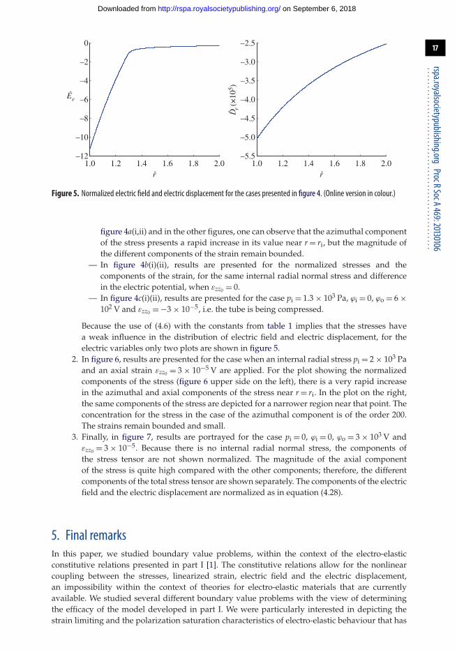
Figure 5. Normalized electric field and electric displacement for the cases presented in figure 4. (Online version in colour.)

figure 4a(i,ii) and in the other figures, one can observe that the azimuthal componentof the stress presents a rapid increase in its value near r = ri, but the magnitude ofthe different components of the strain remain bounded.

— In figure 4b(i)(ii), results are presented for the normalized stresses and thecomponents of the strain, for the same internal radial normal stress and differencein the electric potential, when εzz0 = 0.

— In figure 4c(i)(ii), results are presented for the case pi = 1.3 × 103 Pa, ϕi = 0, ϕo = 6 ×102 V and εzz0 = −3 × 10−5, i.e. the tube is being compressed.

Because the use of (4.6) with the constants from table 1 implies that the stresses havea weak influence in the distribution of electric field and electric displacement, for theelectric variables only two plots are shown in figure 5.

2. In figure 6, results are presented for the case when an internal radial stress pi = 2 × 103 Paand an axial strain εzz0 = 3 × 10−5 V are applied. For the plot showing the normalizedcomponents of the stress (figure 6 upper side on the left), there is a very rapid increasein the azimuthal and axial components of the stress near r = ri. In the plot on the right,the same components of the stress are depicted for a narrower region near that point. Theconcentration for the stress in the case of the azimuthal component is of the order 200.The strains remain bounded and small.

3. Finally, in figure 7, results are portrayed for the case pi = 0, ϕi = 0, ϕo = 3 × 103 V andεzz0 = 3 × 10−5. Because there is no internal radial normal stress, the components ofthe stress tensor are not shown normalized. The magnitude of the axial componentof the stress is quite high compared with the other components; therefore, the differentcomponents of the total stress tensor are shown separately. The components of the electricfield and the electric displacement are normalized as in equation (4.28).

5. Final remarksIn this paper, we studied boundary value problems, within the context of the electro-elasticconstitutive relations presented in part I [1]. The constitutive relations allow for the nonlinearcoupling between the stresses, linearized strain, electric field and the electric displacement,an impossibility within the context of theories for electro-elastic materials that are currentlyavailable. We studied several different boundary value problems with the view of determiningthe efficacy of the model developed in part I. We were particularly interested in depicting thestrain limiting and the polarization saturation characteristics of electro-elastic behaviour that has


18


..................................................


1.0 1.5 2.0

1.0 1.5 2.0

–100

0

100

200

1.00 1.02 1.04

–100

0

100

200

–5

0

5

10

15

r-

r- r-

(×10

–5)

t-rrt-qqt-zz

t-rrt-qqt-zz

erreqqezz

Figure 6. Normalized components of the stress and components of the strain, in the case there is no difference in the electricpotential. (Online version in colour.)

–2.5

–2.0

–1.5

–1.0

–0.5

0

–0.10

–0.05

0

0.05

0.10

0

500

1000

1500

2000

2500

1.0 1.2 1.4 1.6 1.8 2.0–4

–3

–2

–1

–6

–4

–2

0

–1.6

–1.4

–1.2

–1.0

–0.8

–0.6

t rr (×

10–3

)( ×

10–9

)

tqq tzz

err

eqq

r-1.0 1.2 1.4 1.6 1.8 2.0

r-1.0 1.2 1.4 1.6 1.8 2.0

r-

E-r

D- r (×

105 )

Figure 7. Results for the case there is no internal pressure applied on the tube. The components of the total stress tensor are inPa. (Online version in colour.)

been observed and we were able to confirm such behaviour. Several boundary value problemswere studied within the context of the constitutive relations. The first class of problems concernedhomogeneous states of stress; and, in this case, the response of a slab in a state of uniformstress subject to traction, shear and an electric field was analysed. The second class of problems


19


..................................................


concerned inhomogeneous states of stress, and for such states of stress, we studied the responseof a thin circular plate and a long cylindrical tube subject to inflation and an electric field. Wewere able to show that the bodies exhibited limiting strain and saturation of the polarization thatis observed in such electro-elastic bodies.

R.B. expresses his gratitude for the financial support provided by FONDECYT (Chile) under grant no.1120011. K.R.R. thanks the National Science Foundation and the Office of Naval Research for support of thiswork.

References1. Bustamante R, Rajagopal KR. 2013 On a new class of electro-elastic bodies. I. Proc. R. Soc. A

469, 20120521. (doi:10.1098/rspa.2012.0521)2. Rajagopal KR. 2003 On implicit constitutive theories. Appl. Math. 48, 279–319. (doi:10.1023/

A:1026062615145)3. Rajagopal KR. 2007 The elasticity of elasticity. Z. Angew. Math. Phys. 58, 309–317. (doi:10.1007/

s00033-006-6084-5)4. Rajagopal KR. 2011 Conspectus of concepts of elasticity. Math. Mech. Solids 16, 536–562.

(doi:10.1177/1081286510387856)5. Truesdell CA, Noll W. 2004 The non-linear field theories of mechanics. (ed. SS Antman), 3rd edn.

Berlin, Germany: Springer.6. Rajagopal KR, Srinivasa AR. 2007 On the response of non-dissipative solids. Proc. R. Soc. A

463, 357–367. (doi:10.1098/rspa.2006.1760)7. Rajagopal KR, Srinivasa AR. 2009 On a class of non-dissipative solids that are not hyperelastic.

Proc. R. Soc. A 465, 493–500. (doi:10.1098/rspa.2008.0319)8. Chadwick P. 1999 Continuum mechanics: concise theory and problems. Mineola, NY: Dover

Publications Inc.9. Truesdell CA, Toupin R. 1960 The classical field theories. In Handbuch der Physik, vol. III/1

(S. Flüge ed.). Berlin, Germany: Springer.10. Kovetz A. 2000 Electromagnetic theory. Oxford, UK: Oxford University Press.11. Bustamante R, Dorfmann A, Ogden RW. 2009 On electric body forces and Maxwell stresses in

an electroelastic solid. Int. J. Eng. Sci. 47, 1131–1141. (doi:10.1016/j.ijengsci.2008.10.010)12. Dorfmann A, Ogden RW. 2005 Nonlinear electroelasticity. Acta Mech. 174, 167–183.

(doi:10.1007/s00707-004-0202-2)13. Dorfmann A, Ogden RW. 2006 Nonlinear electroelastic deformations. J. Elast. 82, 99–127.

(doi:10.1007/s10659-005-9028-y)14. Spencer AJM. 1971 Theory of invariants. In Continuum physics, vol. 1 (ed. AC Eringen)

pp. 239–353. New York, NY: Academic Press.15. Rajagopal KR, Ruzicka M. 2001 Mathematical modeling of electrorheological materials.

Contin. Mech. Thermodyn. 13, 59–78. (doi:10.1007/s001610100034)16. Maugin GA. 1988 Continuum mechanics of electromagnetic solids. North Holland, Amsterdam.17. Bustamante R, Dorfmann A, Ogden RW. 2011 Numerical solution of finite geometry

boundary-value problems in nonlinear magnetoelasticity. Int. J. Solids Struct. 48, 874–883.(doi:10.1016/j.ijsolstr.2010.11.021)

18. Bustamante R, Dorfmann A, Ogden RW. 2007 A nonlinear magnetoelastic tube underextension and inflation in an axial magnetic field: numerical solution. J. Eng. Math. 59, 139–153.(doi:10.1007/s10665-006-9088-4)

19. Vu DK, Steinmann P. 2010 A 2-D coupled BEM-FEM simulation of electro-elastostatics at largestrain. Comput. Methods Appl. Mech. Eng. 199, 1124–1132. (doi:10.1016/j.cma.2009.12.001)

20. Singh M, Pipkin AC. 1966 Controllable states of elastic dielectrics. Arch. Ratio. Mech. Anal. 21,169–210. (doi:10.1007/BF00253488)

21. Bustamante R. 2009 A variational formulation for a boundary value problem consideringan electro-sensitive elastomer interacting with two bodies. Mech. Res. Commun. 36, 791–795.(doi:10.1016/j.mechrescom.2009.05.009)

22. McMeeking RM, Landis CM. 2005 Electrostatics forces and stored energy for deformabledielectric materials. J. Appl. Mech. T ASEM 72, 581–590. (doi:10.1115/1.1940661)

23. Bustamante R, Dorfmann A, Ogden RW. 2009 Nonlinear electroelastostatics: a variationalframework. Z. Angew. Math. Phys. 60, 154–177. (doi:10.1007/s00033-007-7145-0)

http://dx.doi.org/doi:10.1098/rspa.2012.0521

http://dx.doi.org/doi:10.1023/A:1026062615145

http://dx.doi.org/doi:10.1023/A:1026062615145

http://dx.doi.org/doi:10.1007/s00033-006-6084-5


http://dx.doi.org/doi:10.1177/1081286510387856



http://dx.doi.org/doi:10.1016/j.ijengsci.2008.10.010


http://dx.doi.org/doi:10.1007/s10659-005-9028-y

http://dx.doi.org/doi:10.1007/s001610100034

http://dx.doi.org/doi:10.1016/j.ijsolstr.2010.11.021


http://dx.doi.org/doi:10.1016/j.cma.2009.12.001

http://dx.doi.org/doi:10.1007/BF00253488

http://dx.doi.org/doi:10.1016/j.mechrescom.2009.05.009

http://dx.doi.org/doi:10.1115/1.1940661



20

rspa.royalsocietypublishing.orgProcR

.................................


24. Bustamante R, Rajagopal KR. 2011 Solutions of some simple boundary value problemswithin the context of a new class of elastic materials. Int. J. Nonlinear Mech. 46, 376–386.(doi:10.1016/j.ijnonlinmec.2010.10.002)

25. Ortiz A, Bustamante R, Rajagopal KR. 2012 A numerical study of a plate with a hole for a newclass of elastic bodies. Acta Mech. 223, 1971–1981. (doi:10.1007/s00707-012-0690-4)

26. Bustamante R. 2010 Transversely isotropic nonlinear magneto-active elastomers. Acta Mech.210, 183–214. (doi:10.1007/s00707-009-0193-0)

27. Saada AS. 1993 Elasticity: theory and application, 2nd edn. Malabar, FA: KriegerPublishing Company.

28. Steinmann P, Vu DK. 2012 Computational challenges in the simulation of nonlinearelectroelasticity. Comp. Assisted Methods Eng. Sci. 19, 199–212. (doi:10.1007/978-3-7091-0701-0_5)

29. COMSOL Multiphysics, v. 3.4, 2007. Palo Alto, CA: Comsol Inc.

SocA469:20130106.................

http://dx.doi.org/doi:10.1016/j.ijnonlinmec.2010.10.002



http://dx.doi.org/doi:10.1007/978-3-7091-0701-0_5

http://dx.doi.org/doi:10.1007/978-3-7091-0701-0_5


on June 26, 2018 Onanewclassof electro...

Documents

Transcript of on June 26, 2018 Onanewclassof electro...