NOTES ON “INTRODUCTION TO BIOMEDICAL IMAGING”

BY ANDREW WEBB

SANDRO NUNES TÉCNICAS DE IMAGIOLOGIA

Prof. Patrícia Figueiredo

1

1. X-Ray Imaging and Computed Tomography

1.1. General Principles of Imaging with X-Rays

X-Ray Imaging – transmission-based technique in which X-rays from a source pass through

the patient and are detected either by film or an ionization chamber on the opposite side of the

body. Contrast in the image between different tissues arises from differential attenuation of X-

rays in the body.

Computed Tomography – the source and detectors rotate together around the patient,

producing a series of one-dimensional projections at a number of different angles. This data is

reconstructed to give a two-dimensional image. The x-ray source is collimated to interrogate a

thin slice through the patient. It has a very high spatial resolution (~1mm).

2

1.2. X-ray Production

The x-ray source is the most important component in determining the image quality:

1.2.1. X-ray Source

The main structure of the X-ray source (also called tube) is shown below:

Production of X-rays involves accelerating a beam of electrons to strike the surface of a

metal target. The X-ray tube has 2 electrodes: a negatively charged cathode (electron source) –

filament of coiled tungsten wire - and a positively charged anode (metal target).

An electric current passes through the cathode, heating it (~2200ºC) and causing electrons

to move away from the metallic surface (thermionic emission). The tube potential causes the

free electrons to accelerate towards the anode. Since the spatial resolution is determined by the

effective focal spot size, the cathode is designed to produce a tight, uniform beam of electrons.

To do this, a negatively charged focusing cup is placed around the cathode:

Moreover, the anode is beveled in order to produce a small effective focal spot size:

𝑓 = 𝐹𝑠𝑖𝑛(𝜃)

3

The electrons striking the anode lose their kinetic energy, which is converted into X-rays.

The anode must be made of a metal with high melting point and good thermal conductivity

(usually tungsten).

1.2.2. X-ray tube current, tube output and beam intensity

Tube potential: 15-150kV (rectified alternating voltage, characterized by the maximum

value, kilovolts peak or accelerating voltage - kVp).

Tube current: 50-1000mA (depends on kVp)

Tube output: tube current × tube potential. We need a high tube output in order to

decrease the exposure time. It depends on:

- kVp

- Vacuum in the tube (reduces interactions between electrons and molecules and

increase electrons’ velocity)

Tube power rating: maximum power dissipated in an exposure of 0.1s. Limited by anode

heating, which can be reduced by causing it to rotate at roughly 3000 rpm.

Intensity of the X-ray beam: power incident per unit area (J/m2). It depends on the

number (𝛼 current) and energy of the X-rays (𝛼 kVp2)

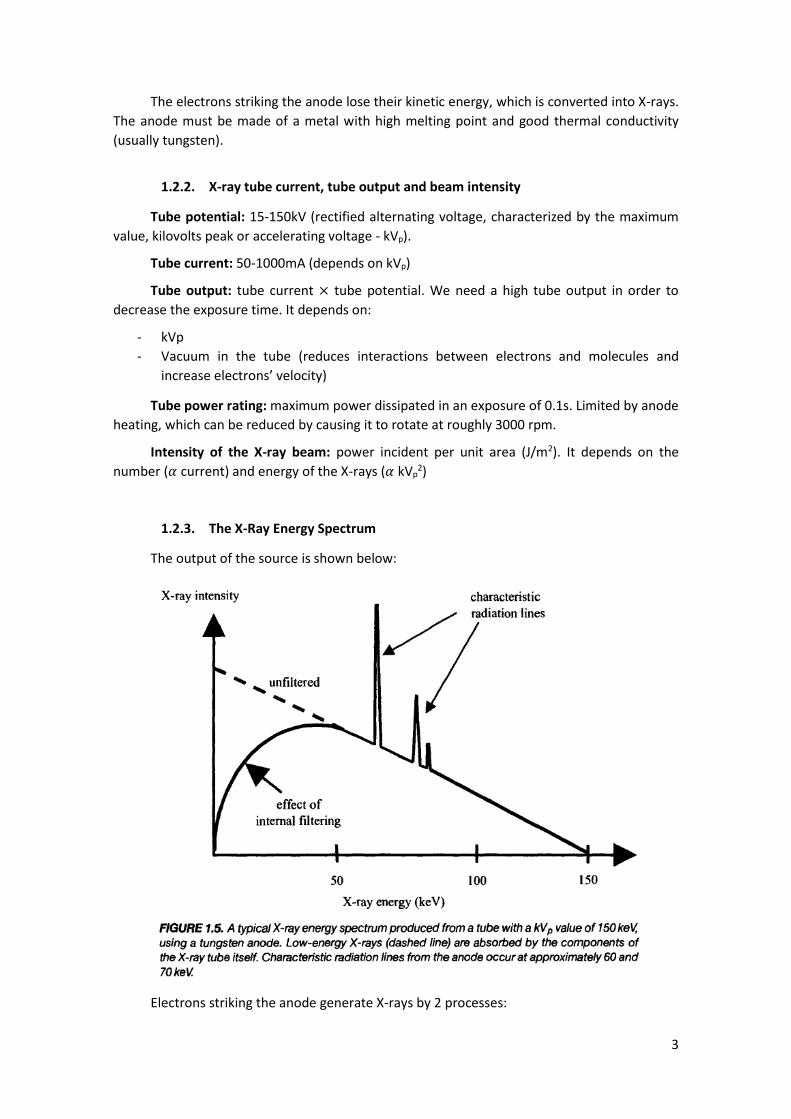
1.2.3. The X-Ray Energy Spectrum

The output of the source is shown below:

Electrons striking the anode generate X-rays by 2 processes:

4

-Bremsstrahlung: generated when an electron is deflected by the tungsten nucleus, losing

kinetic energy which is emitted as an X-ray. The Bremsstrahlung radiation has a wide range of

energies, with a maximum corresponding to the case where all the electron’s kinetic energy is

converted into a single X-ray (with energy kVp). It is characterized by a linear decrease in X-ray

intensity with increasing X-ray energy, however many low energy X-rays are absorbed within the

tube (additional external filters are used because low energy X-rays would be incapable of

passing through the patient, adding to the dose unnecessarily).The efficiency, 𝜂, of the

Bremsstrahlug is given by:

𝜂 = 𝑘(𝑘𝑉𝑝)𝑍

k – constant related to the target material

Z – atomic number of the target material

-Characteristic Radiation: shown as sharp peaks. It is emitted when an accelerated

electron hits an electron in the inner shell of the tungsten atom, causing it to be ejected. An

electron from the outer shell fills the hole, which causes a loss in potential, emitted as an X-ray.

Only happens for incoming electrons with energy > 70 keV.

1.3. Interactions of X-rays with tissue

The X-ray can be classified according to the type of interaction:

- Primary interaction: passes through the body with no interaction.

- Secondary interaction: scattered radiation, whose trajectory between source and

detector was altered. Caused by coherent and Compton scattering.

- Absorbed radiation: absorbed radiation that does not reach the detector. Caused by

photoelectric interactions.

1.3.1. Coherent Scattering

Also called Rayleigh scattering. The radiation is absorbed by the tissue’s atoms and then

emitted in a random direction. Reduces the quantity of X-rays reaching the detectors and alters

their trajectory.

1.3.2. Compton Scattering

Refers to the interaction between an incident X-ray and a loosely bound electron in an

outer shell of an atom in tissue. A fraction of the X-ray energy is transferred to the electron, the

electron is ejected and the X-ray is deflected from its original path. The difference in energy is

very small, which means that this radiation is detected with approximately the same efficiency

as primary radiation. Also, it does not depend on atomic number, thus it is absorbed the same

way in different tissues.

1.3.3. Photoelectric Effect

The energy of the incident X-ray is absorbed by an atom, with a tightly bound electron

being emitted from the K or L shells. A second electron with a higher energy level then fills the

hole, emitting a characteristic X-ray with very low range that does not reach the detector. For

an incident energy just higher than K-shell, the probability of photoelectric interactions is very

high and is given by:

5

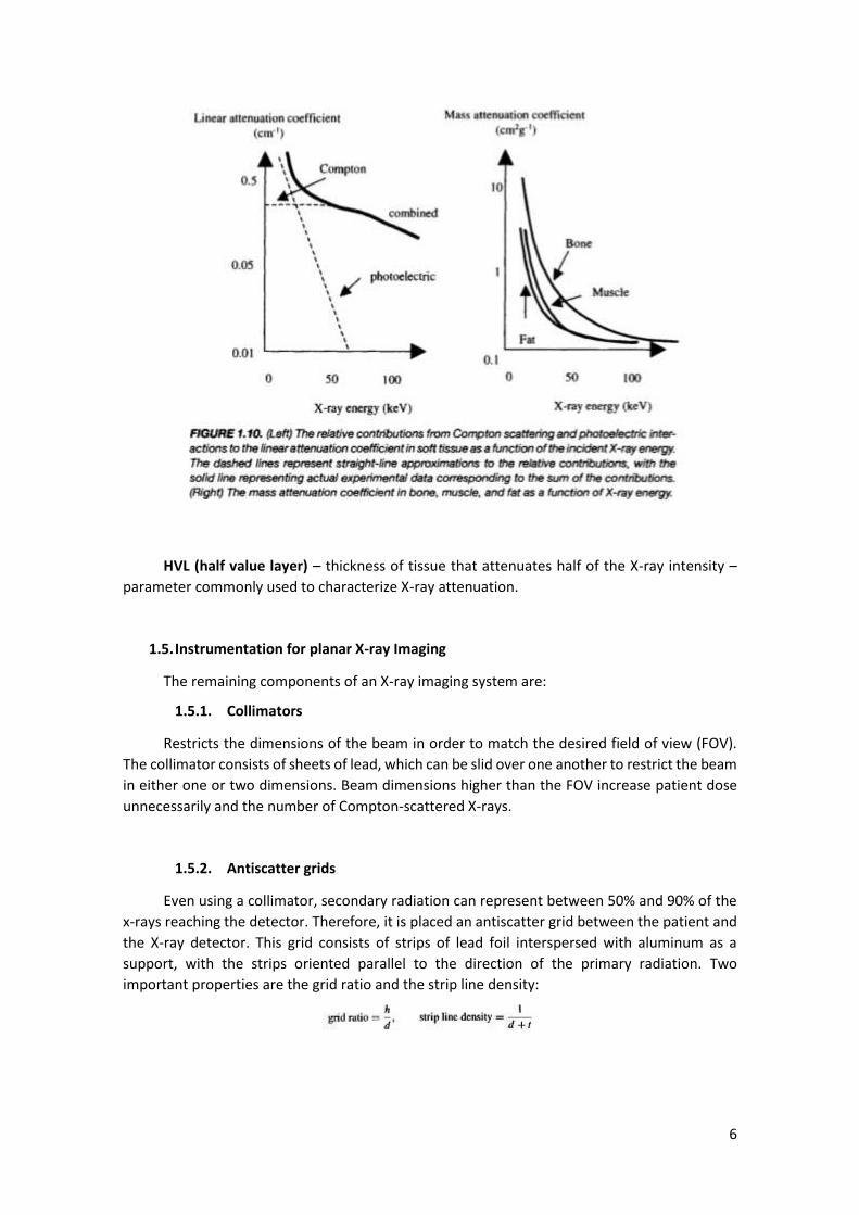
1.4. Linear and mass attenuation coefficients of X-rays in tissue

Attenuation of the X-ray beam through tissue is given by:

𝜇 – linear attenuation coefficient

The value of 𝜇 is given by:

Contributions of photoelectric interactions dominate at lower energies, whereas

Compton scattering is more important at higher energies. X-ray attenuation is often

characterized by mass attenuation coefficient which is equal to the linear attenuation coefficient

divided by the density of the tissue. We can see from the graph below (right) that, at higher

energies, little differentiation is possible because the number of photoelectric interactions

decreases.

6

HVL (half value layer) – thickness of tissue that attenuates half of the X-ray intensity –

parameter commonly used to characterize X-ray attenuation.

1.5. Instrumentation for planar X-ray Imaging

The remaining components of an X-ray imaging system are:

1.5.1. Collimators

Restricts the dimensions of the beam in order to match the desired field of view (FOV).

The collimator consists of sheets of lead, which can be slid over one another to restrict the beam

in either one or two dimensions. Beam dimensions higher than the FOV increase patient dose

unnecessarily and the number of Compton-scattered X-rays.

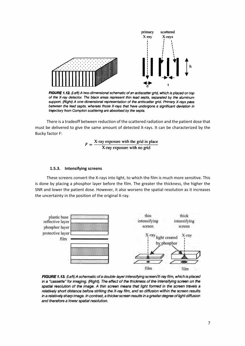
1.5.2. Antiscatter grids

Even using a collimator, secondary radiation can represent between 50% and 90% of the

x-rays reaching the detector. Therefore, it is placed an antiscatter grid between the patient and

the X-ray detector. This grid consists of strips of lead foil interspersed with aluminum as a

support, with the strips oriented parallel to the direction of the primary radiation. Two

important properties are the grid ratio and the strip line density:

7

There is a tradeoff between reduction of the scattered radiation and the patient dose that

must be delivered to give the same amount of detected X-rays. It can be characterized by the

Bucky factor F:

1.5.3. Intensifying screens

These screens convert the X-rays into light, to which the film is much more sensitive. This

is done by placing a phosphor layer before the film. The greater the thickness, the higher the

SNR and lower the patient dose. However, it also worsens the spatial resolution as it increases

the uncertainty in the position of the original X-ray.

8

1.5.4. X-ray film

The presence of lighter regions is due to a chemical reaction of silver particles in the film

to metallic silver. This reaction is reduced in the areas where light hits the film, so the degree of

“blackening” depends on the intensity and time of the light hitting a specific area. This

blackening is measured by the optical density (OD):

Ii – intensity of the light incident on.

It – intensity of the light transmitted through the X-ray film.

1.6. X-Ray image characteristics

1.6.1. Signal to Noise Ratio

SNR is proportional to the statistical variance in the number of X-rays per unit area

(quantum mottle). Since this variance is characterized by a Poisson distribution, SNR is

proportional to the square root of the number of detected X-rays per unit area (N). It is affected

by:

- X-ray tube voltage: the higher the kVp, the higher high-energy X-rays produced and

thus, the number of X-rays reaching the film (↑1)

- X-ray tube current (↑)

- X-ray exposure time (↑)

- Intensifying screen thickness (↑)

- X-ray filtration (↓)

- Object thickness (↓)

- Antiscatter grid ratio (↓)

1.6.2. Spatial Resolution

The main factors affecting it are:

- Effective focal spotsize (↑2)

- Magnification factor (↑)

- Film speed (↑)

- Intensifying screen thickness (↑)

The resultant spatial resolution is given by:

1 The arrows represent what happens to SNR if we increase the value of each given factor. 2 ↑ means higher R, the minimum distance which can be resolved, this is, worse resolution.

9

1.6.3. Contrast to Noise Ratio

Refers to the difference in signal intensity from various regions of the body (for example

the difference between the SNR of bone and soft tissue). It is affected by all the factors that

affect SNR and R, in addition to:

- Energy of the X-ray: if high energies are used, Compton scattering dominates (↓)

- FOV: for values between 10cm and 30cm, the proportion of Compton scattering

reaching the detector increases linearly. After that, it is constant.

- Geometry of the antiscatter grid

1.7. X-ray contrast agents

X-ray contrast agents are chemicals that are introduced in the body to increase image

contrast. Some examples are the barium sulfate and the iodine-based X-ray contrast agents.

These chemicals have a particular K-edge energy that can be used to distinguish the tissues on

which they accumulate from the surroundings.

1.8. X-Ray Imaging methods

The main imaging techniques that use X-rays are:

1.8.1. X-ray angiography

Angiography techniques produce images that show selectively the blood vessels in the

body. Iodine-based contrast agents are injected into the bloodstream to improve contrast. A

related imaging technique called digital subtraction angiography consists on taking an image

before the agent is administered and one after, and then compute the difference (yielding very

high contrast).

1.8.2. X-ray fluoroscopy

X-ray fluoroscopy is a continuous imaging technique using X-rays with very low energies

(used, for example, for placement of stents and catheters). Since very low energies cause low

SNR because of the quantum mottle, a fluoroscopic image intensifier (CsI:Na) is used to improve

the SNR. A fluorescent screen is used to continuously monitor the area of interest.

1.8.3. Dual-Energy Imaging

Technique that produces two separate images corresponding to soft tissue and bone

(used for imaging the chest region). There are 2 ways of performing dual-energy imaging:

- Two X-ray exposures, one applied immediately after the other, with different values of

kVp;

- Single exposure and 2 detectors. The detector placed directly beneath the patient

absorbs low energy X-rays and hardens the beam detected by the second detector.

Therefore, the image from the first detector corresponds to a low energy x-ray, high

10

contrast image, and that from the second, to a high energy x-ray, low contrast image. If

more beam hardening is required, a copper filter can be put in front of the second

detector.

1.9. Clinical applications of X-ray imaging

Apart from the ones described above, there are additional applications of X-ray imaging:

1.9.1. Mammography

X-ray mammography is used to detect small lesions in the breasts. It requires very high

spatial resolution and CNR to detect the microcalcifications (<1mm).

- A low dosage is also important to avoid tissue damage (a molybdenum filter is used to

remove high energies, which also improves CNR);

- Fast intensifying screen/film combinations are necessary to allow the use of low Kvp to

optimize SNR;

- Large source to detector distance and small focal spot size to increase resolution.

1.10. Computed Tomography

CT enables the acquisition of 2D thin slices, which can be obtained in order to reconstruct

a 3D volume. These 2D slices are reconstructed from a series of 1 dimensional projections of the

object acquired at different angles. The detectors, which are situated opposite to the x-ray

source, detect the total number of x-rays transmitted through the patient, producing a one

dimensional projection. The signal intensities in this projection are dictated by the two

dimensional distribution of the tissue attenuation coefficients within the slice. The X-ray source

and the detectors are then rotated by a certain angle and the measurements are repeated. The

image is reconstructed by a process termed backprojection.

1.10.1. Scanner instrumentation

The basic operation of a 1st generation scanner is shown below:

11

The image acquired this way has M X N points. The spatial resolution could be increased

by using finer translational steps or the angular increments, up to a value limited by the effective

x-ray focal spot size.

The 2nd generation replaced the single beam by a fan beam and used multiple detectors,

which reduced the scanning time. It required the development of fan-beam backprojection.

The 3rd generation uses a much wider x-ray fan beam (45º) and an increased number of

detectors (between 512 and 768). Two collimators are used to restrict the fan beam and the

slice thickness (1-5mm). The rotation covers 360º.

In the 4th generation detectors, a complete ring of detectors surrounds the patient. No

decrease in scanning time.

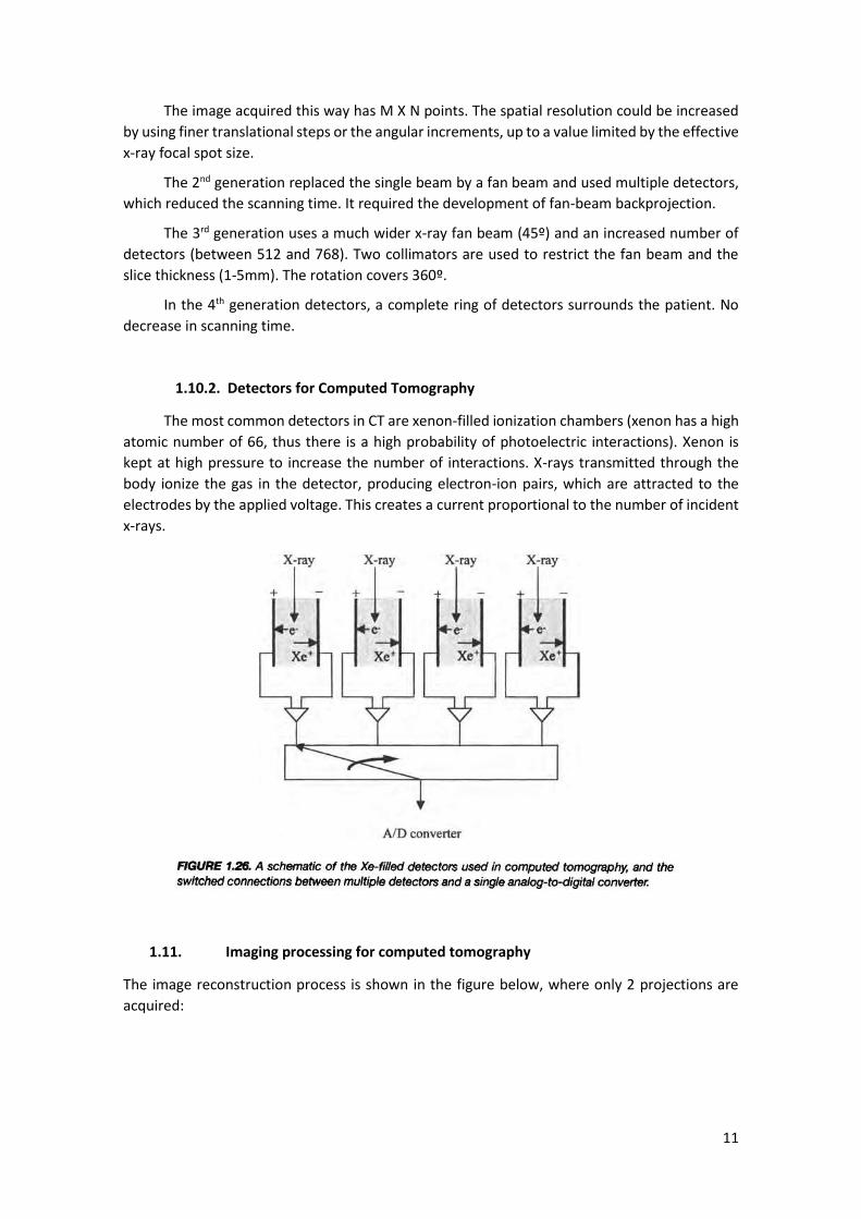
1.10.2. Detectors for Computed Tomography

The most common detectors in CT are xenon-filled ionization chambers (xenon has a high

atomic number of 66, thus there is a high probability of photoelectric interactions). Xenon is

kept at high pressure to increase the number of interactions. X-rays transmitted through the

body ionize the gas in the detector, producing electron-ion pairs, which are attracted to the

electrodes by the applied voltage. This creates a current proportional to the number of incident

x-rays.

1.11. Imaging processing for computed tomography

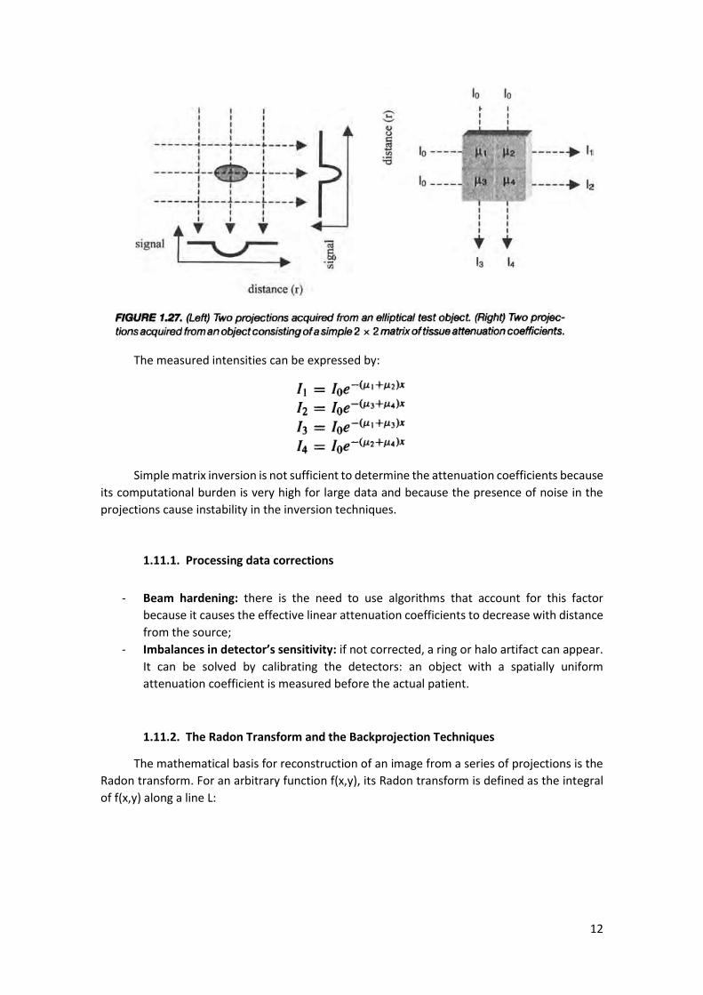
The image reconstruction process is shown in the figure below, where only 2 projections are

acquired:

12

The measured intensities can be expressed by:

Simple matrix inversion is not sufficient to determine the attenuation coefficients because

its computational burden is very high for large data and because the presence of noise in the

projections cause instability in the inversion techniques.

1.11.1. Processing data corrections

- Beam hardening: there is the need to use algorithms that account for this factor

because it causes the effective linear attenuation coefficients to decrease with distance

from the source;

- Imbalances in detector’s sensitivity: if not corrected, a ring or halo artifact can appear.

It can be solved by calibrating the detectors: an object with a spatially uniform

attenuation coefficient is measured before the actual patient.

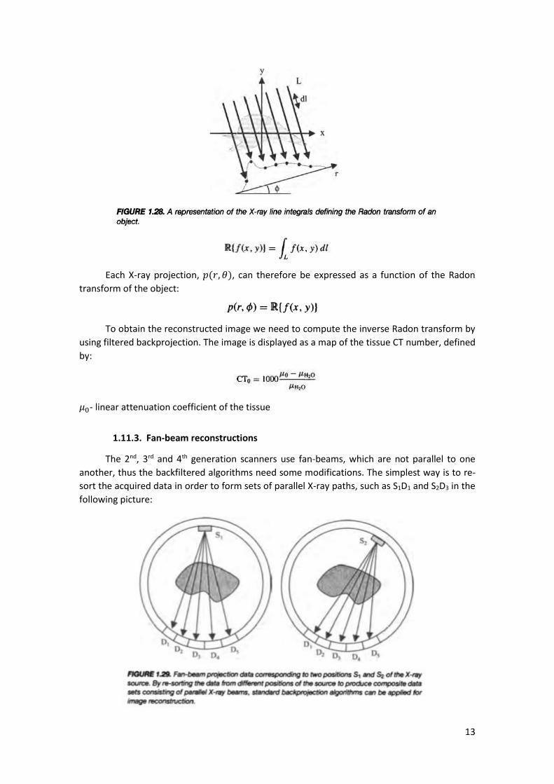
1.11.2. The Radon Transform and the Backprojection Techniques

The mathematical basis for reconstruction of an image from a series of projections is the

Radon transform. For an arbitrary function f(x,y), its Radon transform is defined as the integral

of f(x,y) along a line L:

13

Each X-ray projection, 𝑝(𝑟, 𝜃), can therefore be expressed as a function of the Radon

transform of the object:

To obtain the reconstructed image we need to compute the inverse Radon transform by

using filtered backprojection. The image is displayed as a map of the tissue CT number, defined

by:

𝜇0- linear attenuation coefficient of the tissue

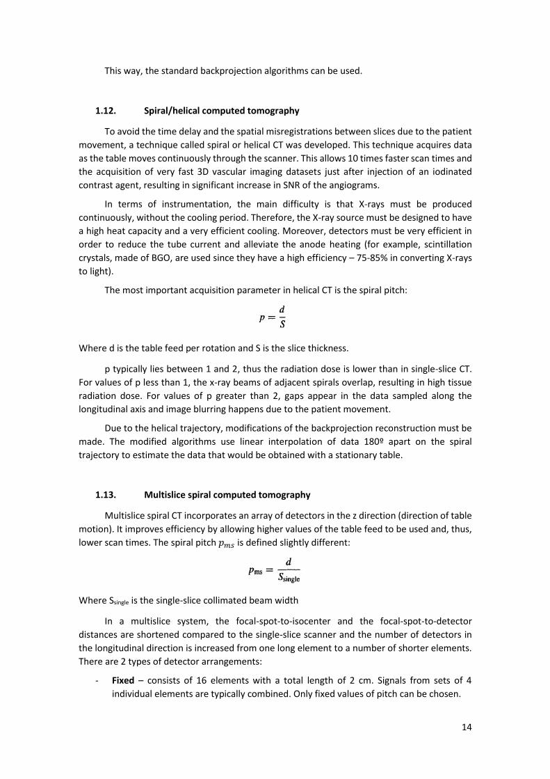
1.11.3. Fan-beam reconstructions

The 2nd, 3rd and 4th generation scanners use fan-beams, which are not parallel to one

another, thus the backfiltered algorithms need some modifications. The simplest way is to re-

sort the acquired data in order to form sets of parallel X-ray paths, such as S1D1 and S2D3 in the

following picture:

14

This way, the standard backprojection algorithms can be used.

1.12. Spiral/helical computed tomography

To avoid the time delay and the spatial misregistrations between slices due to the patient

movement, a technique called spiral or helical CT was developed. This technique acquires data

as the table moves continuously through the scanner. This allows 10 times faster scan times and

the acquisition of very fast 3D vascular imaging datasets just after injection of an iodinated

contrast agent, resulting in significant increase in SNR of the angiograms.

In terms of instrumentation, the main difficulty is that X-rays must be produced

continuously, without the cooling period. Therefore, the X-ray source must be designed to have

a high heat capacity and a very efficient cooling. Moreover, detectors must be very efficient in

order to reduce the tube current and alleviate the anode heating (for example, scintillation

crystals, made of BGO, are used since they have a high efficiency – 75-85% in converting X-rays

to light).

The most important acquisition parameter in helical CT is the spiral pitch:

Where d is the table feed per rotation and S is the slice thickness.

p typically lies between 1 and 2, thus the radiation dose is lower than in single-slice CT.

For values of p less than 1, the x-ray beams of adjacent spirals overlap, resulting in high tissue

radiation dose. For values of p greater than 2, gaps appear in the data sampled along the

longitudinal axis and image blurring happens due to the patient movement.

Due to the helical trajectory, modifications of the backprojection reconstruction must be

made. The modified algorithms use linear interpolation of data 180º apart on the spiral

trajectory to estimate the data that would be obtained with a stationary table.

1.13. Multislice spiral computed tomography

Multislice spiral CT incorporates an array of detectors in the z direction (direction of table

motion). It improves efficiency by allowing higher values of the table feed to be used and, thus,

lower scan times. The spiral pitch 𝑝𝑚𝑠 is defined slightly different:

Where Ssingle is the single-slice collimated beam width

In a multislice system, the focal-spot-to-isocenter and the focal-spot-to-detector

distances are shortened compared to the single-slice scanner and the number of detectors in

the longitudinal direction is increased from one long element to a number of shorter elements.

There are 2 types of detector arrangements:

- Fixed – consists of 16 elements with a total length of 2 cm. Signals from sets of 4

individual elements are typically combined. Only fixed values of pitch can be chosen.

15

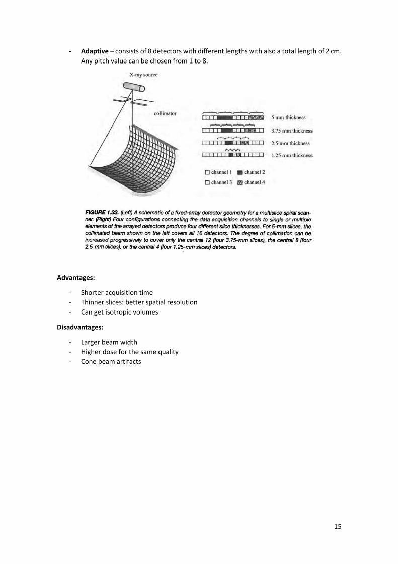
- Adaptive – consists of 8 detectors with different lengths with also a total length of 2 cm.

Any pitch value can be chosen from 1 to 8.

Advantages:

- Shorter acquisition time

- Thinner slices: better spatial resolution

- Can get isotropic volumes

Disadvantages:

- Larger beam width

- Higher dose for the same quality

- Cone beam artifacts

16

2. Nuclear Medicine

2.1. General principles of nuclear medicine

Nuclear medicine images the spatial distribution of radiopharmaceuticals introduced in

the body. It can detect biochemical changes in tissue, serving as a diagnostic to pathological

conditions such as formation of edema, tumor enlargement or metastasis, and changes in the

tissue morphology. These radiopharmaceuticals, termed radiotracers, are compounds linked to

a radioactive element, whose structure determines its distribution in the body. Radiation,

usually in the form of 𝛾-rays, is detected using a gamma camera. The following picture shows

the basic principles and instrumentation involved:

Decay of the radioactive element produces 𝛾-rays, which emanate in all directions.

Attenuation of 𝛾-rays occurs the same way as in X-rays. In order to determine the position of

the source of the 𝛾-rays, a collimator is placed between the patient and the detector so that

only those components of radiation that have a trajectory at an angle close to 90º to the

detector plane are recorded. A scintillation crystal is used to convert the 𝛾-rays into light. These

light photons are in turn converted into an electrical signal by photomultiplier tubes (PMTs). The

image is formed by analyzing the spatial distribution and the magnitude of the electrical signals

from each PMT. Planar nuclear images are characterized as having poor SNR and low spatial

resolution (~5 mm), but extremely high specificity because there is no background radiation in

the body.

17

3D nuclear images can be produced using the principle of tomography. A rotating gamma

camera is used in a technique called single photon emission computed tomography (SPECT). The

most recently developed technique is positron emission tomography (PET), which is based on

positron-emitting radiotracers. This technique has a sensitivity advantage over SPECT of 2 to 3

orders of magnitude.

2.2. Radioactivity

Radioactivity is an intrinsic property of particular isotopes that have unstable nuclei. The

phenomenon of radioactivity refers to the process whereby various forms of radiation are

emitted as result of spontaneous change in the composition of the nucleus. The stability of a

nucleus is dictated by the relationship between Z (nº protons) and A (nº protons +neutrons).

Strong neutron-neutron, proton-neutron and proton-proton forces are attractive over very

short distances, whereas electromagnetic forces between protons are repulsive, and so the

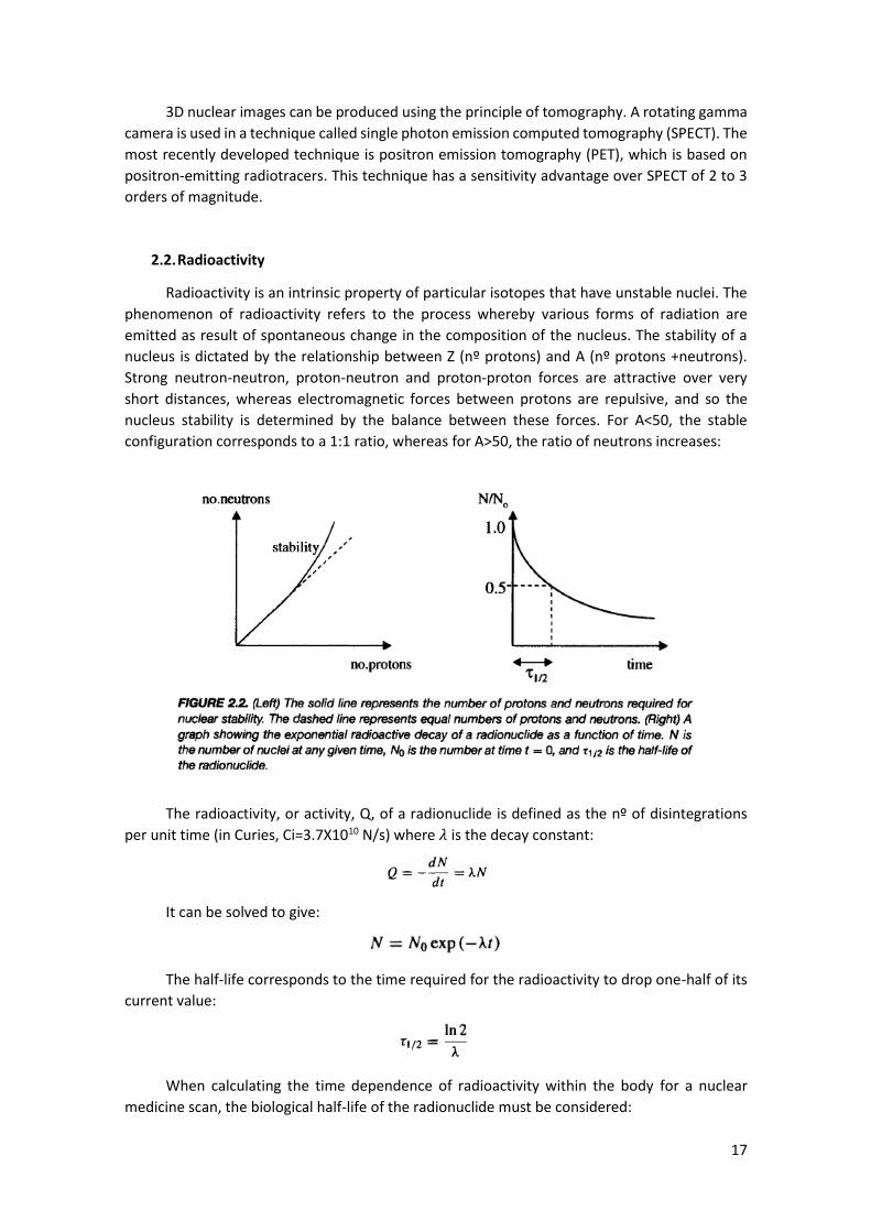
nucleus stability is determined by the balance between these forces. For A<50, the stable

configuration corresponds to a 1:1 ratio, whereas for A>50, the ratio of neutrons increases:

The radioactivity, or activity, Q, of a radionuclide is defined as the nº of disintegrations

per unit time (in Curies, Ci=3.7X1010 N/s) where 𝜆 is the decay constant:

It can be solved to give:

The half-life corresponds to the time required for the radioactivity to drop one-half of its

current value:

When calculating the time dependence of radioactivity within the body for a nuclear

medicine scan, the biological half-life of the radionuclide must be considered:

18

2.3. Production of radionuclides

There are 4 basic methods for producing radionuclides:

- Neutron capture

- Nuclear fission (uses fast high energy neutrons to create 99Mo 133Xe and 131I)

- Charged particle bombardment (uses a cyclotron to accelerate ionized hydrogen or

deuterium gas and create 201Ti, 67Ga, 111In or 123I)

- Radionuclide generators (most common method, via on-site generator)

2.4. Types of radioactive decay

Radioactive elements can decay via a number of mechanisms, of which the most

important in nuclear medicine are:

- 𝛼-particle decay

- 𝛽-particle emission

- 𝛾-ray emission

- Electron emission

The most useful radionuclides are the ones that emit 𝛾-rays or X-rays because these forms

of radiation can pass through tissue and reach the detector. A useful parameter to quantify

attenuation is the HVL.

An 𝛼-particle consists of a helium nucleus. It has a tissue HVL of only a few mm and, thus,

it is not directly related to nuclear medicine. This form of radioactive decay occurs mainly for

radionuclides with Z>150.

A 𝛽-particle is an electron. Radioactive decay occurs via conversion of a neutron into a

proton, with emission of a high energy 𝛽-particle and an antineutrino. Kinetic energy is shared

in a random manner between the 𝛽-particle and the neutrino, and hence the electron has a

continuous range of energies (e.g.: a 1MeV 𝛽-particle has a HVL=0.4 mm while a 5MeV 𝛽-particle

has a HVL=4 mm).

Due to their low HVL, radionuclides that produce 𝛼 and 𝛽 particles cannot be used for

imaging.

No radionuclide can decay solely by 𝛾-ray emission, but certain decay schemes result in

formation of an intermediate species that exists in a metastable state. This is the case of 99mTc,

which is the most widely used:

The energy of the emitted 𝛾-ray for the 99mTc is 140 keV. Below an energy of 100 keV most

𝛾-rays are absorbed in the body via photoelectric interactions. Above 200 keV, 𝛾-rays penetrate

the thin collimator septa, thus the ideal energy range lies between 100 and 200 keV.

19

The final mechanism of radioactive decay is the electron capture (with subsequent 𝛾-ray

or X-ray emission), in which an orbital electron from the K or L shell is captured by the nucleus,

leaving a hole that is occupied by an outer electron. This process produces characteristic X-rays.

For clinical imaging, an ideal radionuclide should have a half-life short enough to limit the

dose to the patient but long enough such that the radioactivity is not exhausted by the time the

nuclide has distributed within the body. The radioactive decay should be via monochromatic 𝛾-

ray emission to a stable nuclear state, without 𝛼 or 𝛽-particle emission.

2.5. Technetium generator

99mTc is the most used radionuclide because:

- Can be produced from an on-site generator

- Half-life of 6.02h

- Very minor 𝛽-particle emission

- HVL of 4.6 cm

The generator consists of an alumina ceramic column with 99Mo on its surface. The 99mTc

is obtained by flowing an eluting solution through the generator, which washes out the 99mTc,

leaving behind the 99Mo. Typically, the technetium is eluded every 24h and the generator is

replaced once a week.

2.6. Biodistribution of the technetium-based agents within the body

The majority of radiopharmaceuticals uses ionic technetium (TC4+), which is bind to a

metal ion according to the target organ.

2.7. Instrumentation: the gamma camera

20

The roles of each component of the gamma camera are listed below:

2.7.1. Collimator

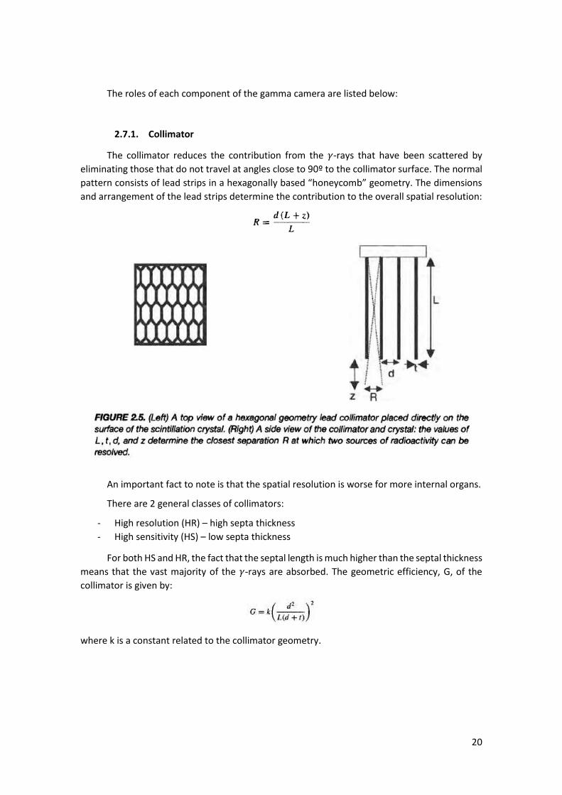
The collimator reduces the contribution from the 𝛾-rays that have been scattered by

eliminating those that do not travel at angles close to 90º to the collimator surface. The normal

pattern consists of lead strips in a hexagonally based “honeycomb” geometry. The dimensions

and arrangement of the lead strips determine the contribution to the overall spatial resolution:

An important fact to note is that the spatial resolution is worse for more internal organs.

There are 2 general classes of collimators:

- High resolution (HR) – high septa thickness

- High sensitivity (HS) – low septa thickness

For both HS and HR, the fact that the septal length is much higher than the septal thickness

means that the vast majority of the 𝛾-rays are absorbed. The geometric efficiency, G, of the

collimator is given by:

where k is a constant related to the collimator geometry.

21

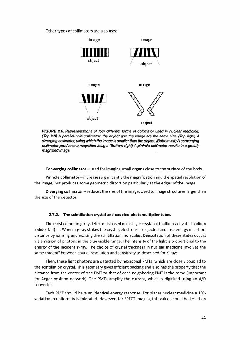
Other types of collimators are also used:

Converging collimator – used for imaging small organs close to the surface of the body.

Pinhole collimator – increases significantly the magnification and the spatial resolution of

the image, but produces some geometric distortion particularly at the edges of the image.

Diverging collimator – reduces the size of the image. Used to image structures larger than

the size of the detector.

2.7.2. The scintillation crystal and coupled photomultiplier tubes

The most common 𝛾-ray detector is based on a single crystal of thallium-activated sodium

iodide, NaI(Ti). When a 𝛾-ray strikes the crystal, electrons are ejected and lose energy in a short

distance by ionizing and exciting the scintillation molecules. Deexcitation of these states occurs

via emission of photons in the blue visible range. The intensity of the light is proportional to the

energy of the incident 𝛾-ray. The choice of crystal thickness in nuclear medicine involves the

same tradeoff between spatial resolution and sensitivity as described for X-rays.

Then, these light photons are detected by hexagonal PMTs, which are closely coupled to

the scintillation crystal. This geometry gives efficient packing and also has the property that the

distance from the center of one PMT to that of each neighboring PMT is the same (important

for Anger position network). The PMTs amplify the current, which is digitized using an A/D

converter.

Each PMT should have an identical energy response. For planar nuclear medicine a 10%

variation in uniformity is tolerated. However, for SPECT imaging this value should be less than

22

1%. In practice, calibration is done using samples of uniform and known radioactivity or, more

recently, through a LED calibration source for each PMT in real time.

2.7.3. The Anger position network and the Pulse Height Analyzer

By comparing the magnitudes of the currents from all of the PMTs, the location of

individual scintillations within the crystal can be estimated. This calculation is done by using an

Anger logic circuit. This network produces four output signals, X+, X-, Y+ and Y-, the relative

magnitudes and signs of which define the location of the scintillation in the crystal. The summed

signal, termed the z-signal, is sent to a pulse-height analyzer (PHA), which compares the z-signal

to a threshold value to determine if it was originated by a scattered 𝛾-ray (for a 99mTC scan, it

corresponds to that produced by a 𝛾-ray with energy 140 keV). The z-signal is accepted if its

energy is inside a certain interval given by the full-width half-maximum (FWHM) of the

photopeak: the narrower the FWHM, the better it is at discriminating between scattered and

unscattered 𝛾-rays. Typically, a 15% interval is used.

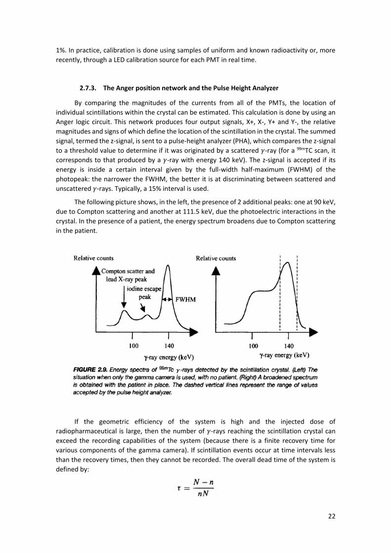
The following picture shows, in the left, the presence of 2 additional peaks: one at 90 keV,

due to Compton scattering and another at 111.5 keV, due the photoelectric interactions in the

crystal. In the presence of a patient, the energy spectrum broadens due to Compton scattering

in the patient.

If the geometric efficiency of the system is high and the injected dose of

radiopharmaceutical is large, then the number of 𝛾-rays reaching the scintillation crystal can

exceed the recording capabilities of the system (because there is a finite recovery time for

various components of the gamma camera). If scintillation events occur at time intervals less

than the recovery times, then they cannot be recorded. The overall dead time of the system is

defined by:

23

where N in the true count rate and n is the observed count rate. Standard gamma cameras

typically have a 20% loss in the number of counts.

2.8. Image characteristics

Nuclear medicine images are characterized by low SNR and poor spatial resolution, but an

extremely high CNR. Postprocessing is used to increase the image SNR, although this further

degrades the spatial resolution.

2.8.1. Signal to Noise Ratio

The number of disintegrations per unit time fluctuates around an average value described

by a Poisson distribution and, thus, SNR is proportional to the square root of the number of

counts (√𝑁). The factors that affect SNR are:

- Radioactive dose administered (↑) – comparing to X-rays, the number of counts is

10000 times lower

- Effectiveness of the radiopharmaceutical at targeting a specific organ (↑)

- Time over which the image is acquired (↑) – limited by radioactive and biological half-

lives

- Sensitivity of the gamma camera (↑) – related to the collimator geometry and the

thickness of the scintillation crystal

- Postacquisition image filtering (↑) – by applying low pass filters (however causes blur)

2.8.2. Spatial Resolution

There are 4 major contributions to the spatial resolution of a nuclear medicine scan:

- Intrinsic spatial resolution of the gamma camera, excluding the collimator (↑) – reflects

the uncertainty in the exact location at which light is produced in the scintillation crystal

due to thickness of the crystal and the Anger position encoder (~3-5 mm).

- Geometry of the collimator

- Degree of Compton scattering (↑) – goes up with depth of the radiopharmaceutical

within the body

- Postacquisition image filtering (↑)

Considering the first 3 terms, the overall spatial resolution is given by:

Typical values are approximately 1-2 cm and 5-8 mm for organs in depth and close to the

surface of the collimator, respectively.

2.8.3. Contrast to Noise Ratio

If there’s no background signal (due to the fact that the radiopharmaceutical did not

distribute out of the targeted area), then CNR ~ SNR. It is affected by:

24

- Compton scattering (↓)

- Partial volume effects (↓) – depends on R

- Postprocessing filtering

2.9. Single photon emission computed tomography

SPECT applies tomographic principles to produce a series of 2D images. Its main image

characteristics are:

- CNR: improved by up to a factor of 5 to 6 times because sources of radioactivity are not

superimposed.

- R: not changed. Approximately Gaussian PSF with FWHM ~1 cm

- SNR: it needs about 5 times as many counts to obtain an equivalent SNR as in planar

scintigraphy (~500,000 counts in brain and ~100,000 counts in myocardium)

It is the standard acquisition modality for myocardial and brain perfusion and for

oncological investigations.

2.9.1. Instrumentation for SPECT

SPECT can be performed using either multidetector or rotating gamma camera systems.

The former has higher sensitivity and spatial resolution but is very complex and expensive,

making it a rare technique in clinic environment. The latter is preferred for routine clinical

imaging because it can also be used for planar scintigraphy. Data is collected from multiple views

as the detector rotates around the patient. An improvement to this setup is to increase the

number of cameras in the system as the sensitivity per slice is proportional to the number of

cameras. Thus, two and three camera systems are commonly used. A 360º rotation is generally

needed in SPECT because the effects of 𝛾-ray scatter and tissue attenuation and the dependence

of the spatial resolution on the source to detector distance all mean that projections acquired

at 180º to one another are not identical. A focused collimator is used to improve sensitivity,

which requires increased complexity of data reconstruction.

The data matrix acquired is usually 64x64 or 128x128 with first allowing better SNR and

the second allowing better spatial resolution. Projections can be acquired in a “stop-and-go”

mode or in a continuous rotation.

2.9.2. Scatter and attenuation correction

In SPECT, scatter correction is needed because we do not have a well-defined 𝛾-ray

geometry due the lack of tight source collimation. Moreover, tissue attenuation has here a

different role: in CT, the reconstructed image is an estimate of the spatial distribution of X-ray

attenuation coefficients, while in SPECT the reconstructed image is an estimate of the spatial

distribution of injected radiopharmaceutical. Thus, spatially dependent 𝛾-ray attenuation gives

rise to artifacts and need to be corrected. If tissue attenuation is not included, a measured SPECT

projection can be represented as:

25

If we add tissue attenuation, then:

This equation is extremely difficult to solve analytically and, thus, it is an important part

of SPECT data processing.

The scatter correction is done by using a dual-energy window detection method: the main

window contains contributions from both scattered and unscatterd 𝛾-rays (fractional width of

20% around 140keV); the subwindow is set to a lower energy (7% around 121keV). The true

primary 𝛾-rays count can be calculated from:

The attenuation correction can be done using 2 different methods. The first assumes that

𝛾-ray attenuation is uniform throughout the entire body. Thus assumption works well for the

brain, but introduces artifacts in cardiac imaging, for example. The second measures the

attenuation distribution using transmission of a reference activity to make a calibration.

2.10. Clinical applications of nuclear medicine

The major clinical applications are the measurement of blood perfusion in the brain, the

diagnosis of tumors in various organs and the assessment of cardiac function.

2.10.1. Brain Imaging

- Planar scintigraphy using DTPA or 99tTc-glucoheptonate, which do not cross the blood

brain barrier (BBB), can be used to determine a rupture of the BBB as there will be a

high concentration of these radiotracers in the brain.

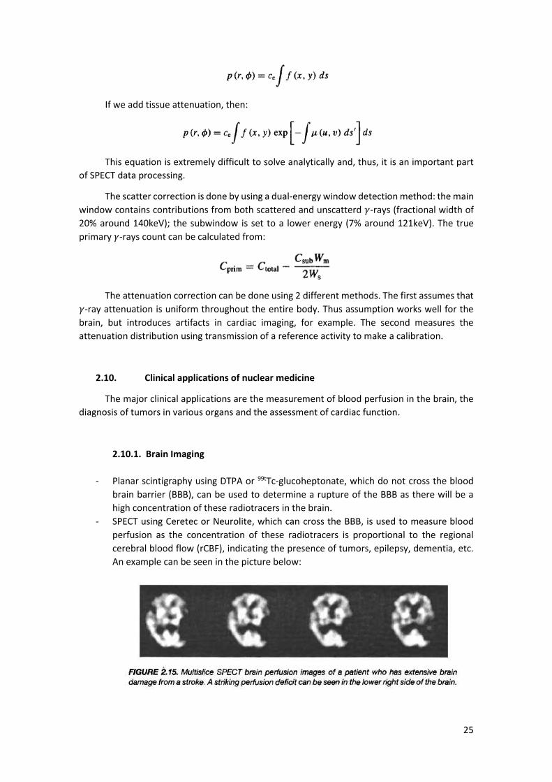
- SPECT using Ceretec or Neurolite, which can cross the BBB, is used to measure blood

perfusion as the concentration of these radiotracers is proportional to the regional

cerebral blood flow (rCBF), indicating the presence of tumors, epilepsy, dementia, etc.

An example can be seen in the picture below:

26

2.10.2. Cardiac Imaging

Cardiac SPECT scans are performed to measure blood flow pattern in the heart and to

detect coronary artery disease and myocardial infarcts. The most common test is the stress test,

used to measure myocardial perfusion and diagnose myocardial ischemia and infarct.

2.11. Positron Emission Tomography

PET, as SPECT, is also a tomographic technique used to measure physiology and function,

rather than gross anatomy. The fundamental difference is that now the radiotracer emits

positrons, which, after annihilation with an electron in the tissue, result in the formation of 2 𝛾-

rays. This fact makes it possible to produce images with much higher SNR and spatial resolution

as we will see.

PET is mainly used in oncology, cardiology and neurology. The main disadvantage is its

high cost and the need to have a cyclotron on-site to produce positron-emitting nuclides.

2.11.1. General principles

The radiotracers used in PET are structural analogs of a biologically active molecule, such

as glucose, in which one or more atoms have been replaced by a radioactive atom. An important

example is the FDG, which contains 18F and [11C]palmitate. Isotopes such as 18F undergo

radioactive decay by emitting a positron, that is, a positively charged electron, and a neutrino:

The positron then annihilates with an electron, resulting in 2 𝛾-rays, each with an energy

of 511 keV, which travel in opposite directions an angle of 180º to one another. Because 2

antiparallel 𝛾-rays are produced and both must be detected, a PET system consists of a complete

ring of scintillation crystals surrounding the patient. Since they are created simultaneously, both

are detected within a certain time window with the 2 crystals that detected them defining a line

along which the annihilation occurred. This process of line definition is called annihilation

coincidence detection (ACD). This difference in localization method is the major reason for the

much higher detection efficiency in PET than in SPECT (moreover, the fact that the 𝛾-ray energy

is much higher means less attenuation, increasing further the sensitivity). The spatial resolution

depends upon a number of factors including the number and size of the individual crystal

detectors (R~3-5 mm).

2.11.2. Radionuclides used for PET

All the radionuclides used in PET are produced by a cyclotron. The most common are 18F, 11C, 15O and 13N.

27

2.11.3. Instrumentation for PET

The major differences are the scintillation crystals needed to detect the 511 keV 𝛾-rays

efficiently and the additional circuitry needed for coincidence detection.

2.11.3.1. Scintillation crystals

They are in large number and are usually formed from bismuth germinate (BGO). The

crystals are coupled to a smaller number PMTs (for cost reasons). Typically, each “block” of

scintillation crystals consists of an 8X8 array cut from a single BGO crystal. Each block is coupled

to 4 PMTs. Four of these blocks are arranged to form a bucket. The full detector ring may have

up to 32 of such buckets. The ideal detector must have a high density and a large effective atomic

number in order to increase the 𝛾-rays detection efficiency by increasing Compton and

photoelectric interactions. The size of the crystal is also important as it affects spatial resolution

(however, crystals too small can cause scatter to adjacent crystals, which reduces resolution;

width for BGO ~1 cm).

2.11.3.2. Annihilation coincidence detection circuitry

The ACD circuitry is designed to maximize the ratio of true-to-false recorded coincidences.

Considered the example in left picture:

A positron is emitted and annihilates with an electron, producing 2 anti-parallel 𝛾-rays.

The first is detected by the crystal number 2 and produces a number of photons. These photons

are converted into an amplified electrical signal at the output of the PMT, which is fed into a

PHA. If the voltage is inside a predefined range, than the PHA generates a logic pulse, which is

sent to the coincidence detector. When the second 𝛾-ray is detected (by the crystal number 10)

28

and produces a voltage that is accepted by the associated PHA, a second logic pulse is sent to

the coincidence detector. This detector sums the 2 logic pulses and passes it through another

PHA, which has a threshold set just under the sum value. If the logic pulses overlap in time, then

the system accepts the 2 𝛾-rays as having evolved from one annihilation and record a line

integral between the 2 crystals.

2.11.4. Image Reconstruction

The process is basically the same as in SPECT, however, prior to reconstruction,

corrections to attenuation and accidental coincidences must be made.

2.11.4.1. Attenuation Correction

The 2 methods available are very similar to the ones described for SPECT.

2.11.4.2. Correction for accidental, multiple and scattered coincidences

The main sources of noise in PET are accidental and scattered coincidences:

The accidental coincidences term is usually much higher. An event of this type is shown

below:

29

The rate at which these accidental coincidences are recordeded is given by:

Where Ri and Rj are the single count rates in the individual detectors i and j.

To correct the accidental coincidences, we can either measure the Ri and Rj or use an

additional parallel timing circuitry.

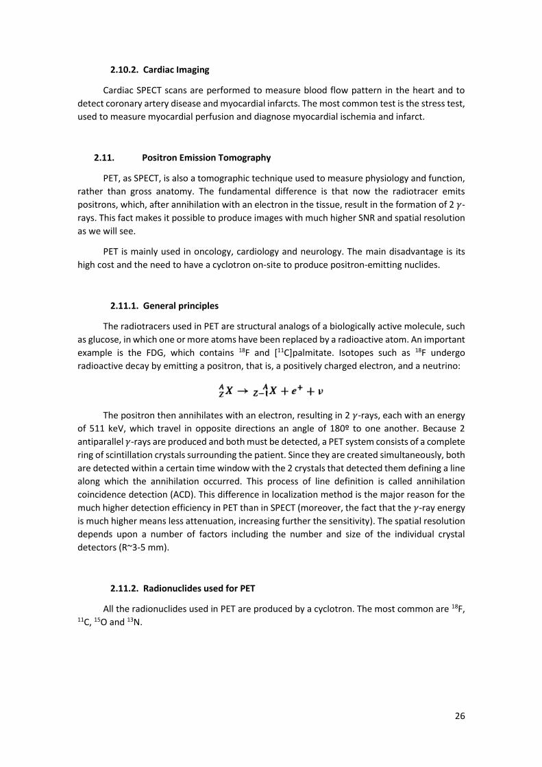
A multiple coincidence represents the combination of a true coincidence with one or more

unrelated events, such as the one in the following picture:

In this case, 2 events are recorded at the same time. Since it is not clear which one should

be accepted, both are discarded, which results in a significant loss of counts and in an effective

deatime for the PET system. The deadtime loss (DTL) is estimated by measuring the number of

triple coincidences and is corrected by the factor:

Scattered coincidences occur if one or both 𝛾-rays suffer scattering before reaching the

detectors. They can be corrected by measuring the amount of scatter in the image in areas

outside the patient, with these values being extrapolated mathematically to estimate the

amount of scatter inside the patient.

2.11.5. Image characteristics

The factors that affect the SNR and CNR are identical to the ones in SPECT (however, there

is no depth dependence on PET). Other factors that affect spatial resolution are:

30

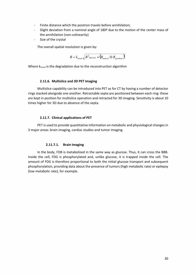
- Finite distance which the positron travels before annihilation;

- Slight deviation from a nominal angle of 180º due to the motion of the center mass of

the annihilation (non-colinearity)

- Size of the crystal

The overall spatial resolution is given by:

Where krecon is the degradation due to the reconstruction algorithm

2.11.6. Multislice and 3D PET Imaging

Multislice capability can be introduced into PET as for CT by having a number of detector

rings stacked alongside one another. Retractable septa are positioned between each ring: these

are kept in position for multislice operation and retracted for 3D imaging. Sensitivity is about 10

times higher for 3D due to absence of the septa.

2.11.7. Clinical applications of PET

PET is used to provide quantitative information on metabolic and physiological changes in

3 major areas: brain imaging, cardiac studies and tumor imaging.

2.11.7.1. Brain Imaging

In the body, FDB is metabolized in the same way as glucose. Thus, it can cross the BBB.

Inside the cell, FDG is phosphorylated and, unlike glucose, it is trapped inside the cell. The

amount of FDG is therefore proportional to both the initial glucose transport and subsequent

phosphorylation, providing data about the presence of tumors (high metabolic rate) or epilepsy

(low metabolic rate), for example.

31

3. Ultrasonic Imaging

3.1. General principles of ultrasonic imaging

Ultrasound imaging operates at frequencies between 1 and 10 MHz, producing images

based on backscattering of mechanical energy from boundaries between tissues and from small

structures within tissue. It can be used to obtain anatomical information (either at surface, using

higher frequencies, or deep in the body, using lower frequencies) or to measure blood flow (via

Doppler shift).

Advantages: Noninvasive, easily portable, inexpensive diagnostic modality, allowing real-

time imaging and high spatial resolution.

Disadvantages: relatively poor soft-tissue contrast and the fact that gas and bone impede

the passage of ultrasound waves.

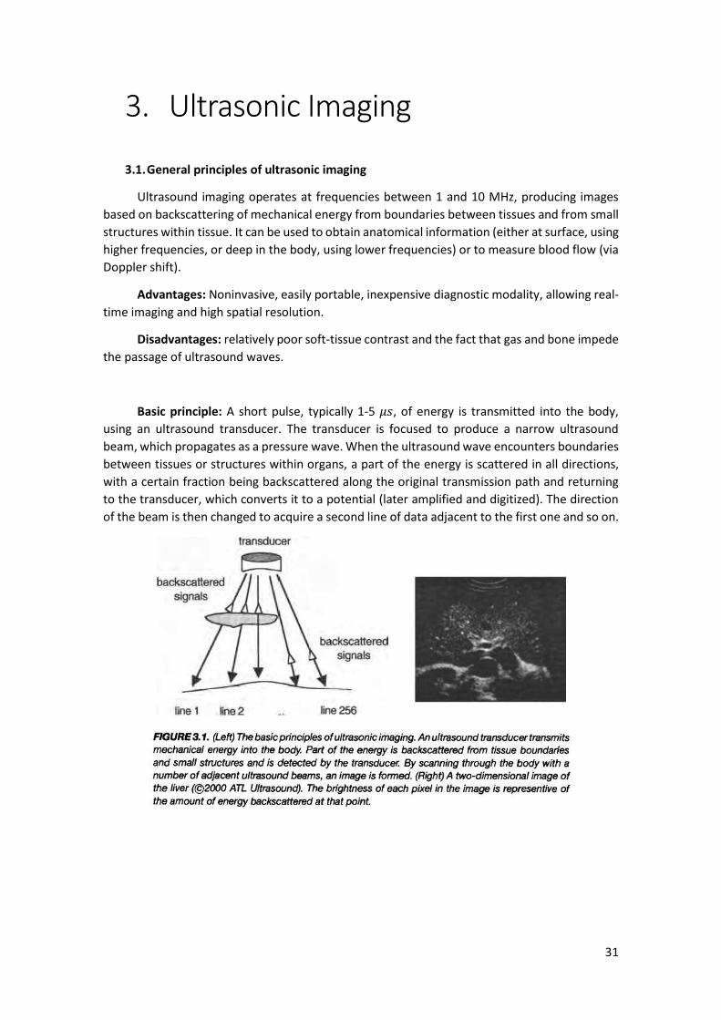
Basic principle: A short pulse, typically 1-5 𝜇𝑠, of energy is transmitted into the body,

using an ultrasound transducer. The transducer is focused to produce a narrow ultrasound

beam, which propagates as a pressure wave. When the ultrasound wave encounters boundaries

between tissues or structures within organs, a part of the energy is scattered in all directions,

with a certain fraction being backscattered along the original transmission path and returning

to the transducer, which converts it to a potential (later amplified and digitized). The direction

of the beam is then changed to acquire a second line of data adjacent to the first one and so on.

32

3.2. Wave propagation and characteristic acoustic impedance

A useful model of tissue is that of a lattice of small particles held together by elastic forces:

As the ultrasound energy passes through the tissue, the particles move very short

distances (W) about a fixed mean position, whereas the ultrasonic energy propagates over much

larger distances. The directions of particle vibration and wave propagation are the same

(longitudinal wave). Assuming a planar wavefront and no loss of energy, the particle

displacement W can be described as a function of the sound velocity by:

The value c depends on the tissue density 𝜌 and compressibility 𝜅:

The particle velocity (much slower than c) in the z direction, 𝑢𝑧, is given by

The pressure, p, of the wave is given by:

Because the transducer undergoes sinusoidal motion, 𝑝(𝑡) and 𝑢𝑧(𝑡) can be described as:

The mean intensity is given by

An important parameter in ultrasonic imaging is the characteristic acoustic impedance Z

of the tissue (analog to Ohm’s Law):

33

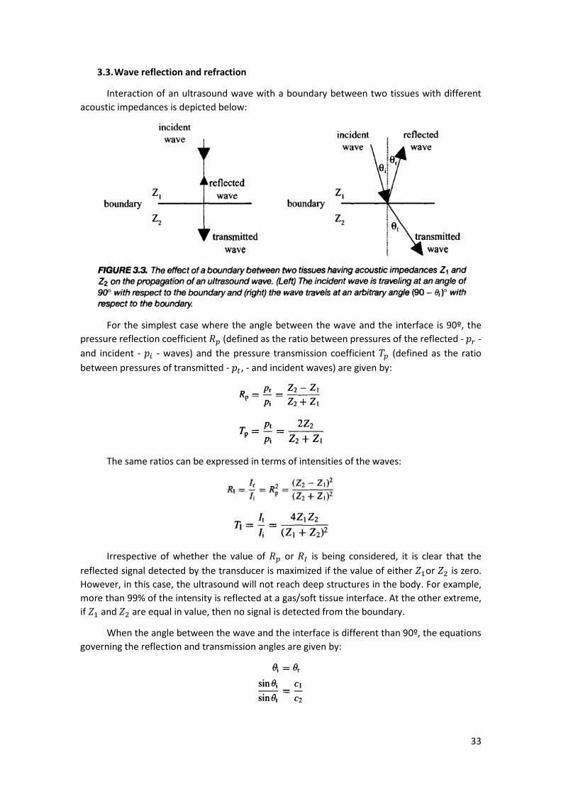
3.3. Wave reflection and refraction

Interaction of an ultrasound wave with a boundary between two tissues with different

acoustic impedances is depicted below:

For the simplest case where the angle between the wave and the interface is 90º, the

pressure reflection coefficient 𝑅𝑝 (defined as the ratio between pressures of the reflected - 𝑝𝑟 -

and incident - 𝑝𝑖 - waves) and the pressure transmission coefficient 𝑇𝑝 (defined as the ratio

between pressures of transmitted - 𝑝𝑡, - and incident waves) are given by:

The same ratios can be expressed in terms of intensities of the waves:

Irrespective of whether the value of 𝑅𝑝 or 𝑅𝐼 is being considered, it is clear that the

reflected signal detected by the transducer is maximized if the value of either 𝑍1or 𝑍2 is zero.

However, in this case, the ultrasound will not reach deep structures in the body. For example,

more than 99% of the intensity is reflected at a gas/soft tissue interface. At the other extreme,

if 𝑍1 and 𝑍2 are equal in value, then no signal is detected from the boundary.

When the angle between the wave and the interface is different than 90º, the equations

governing the reflection and transmission angles are given by:

34

If 𝑐1 ≠ 𝑐2, then the transmitted signal is refracted, which leads to misregistration artifacts.

The pressure and intensity coefficients are given by:

3.4. Energy loss mechanism in tissue

In addition to reflection, ultrasound waves can be attenuated by absorption and

scattering.

3.4.1. Absorption

Absorption refers to the conversion of mechanical energy into heat, which can occur

either by:

- Classical absorption: due to friction between particles as they are displaced by the

passage of the ultrasound wave. Proportional to the square of the wave frequency.

- Relaxation: due to the time 𝜏 taken for a molecule to return to its original position. If

the relaxation time of the tissue is of the same order of the wave period, then the

relaxation mechanism can act against the compression/rarefaction cycle, which leads to

loss of energy.

3.4.2. Scattering

Scattering occurs when the beam encounters tissue irregularities or particles that are the

same size or smaller than the ultrasound wavelength. If the size of the scattering body is small

compared to the wavelength, then scattering is relatively uniform in direction with slightly more

energy being scattered towards the transducer (Rayleigh scattering). It is characterized in terms

of scattering cross section 𝜎𝑠, which depends on the fourth power of wave frequency.

3.4.3. Attenuation

Attenuation is the sum of the scattering and absorption processes. It is characterized by

an exponential decrease in both pressure and intensity of the ultrasound as a function of

propagation distance z:

35

Where the intensity attenuation coefficient 𝜇 and the pressure attenuation coefficient 𝛼

depend linearly on the wave frequency.

3.5. Instrumentation

The instrumentation for ultrasounds consists of:

- Transducer (single-crystal or, more commonly, an array of crystals): converts oscillating

voltage into mechanical vibrations and vice-versa

- Detection electronics: modules for time-gain compensation and beam forming;

- Computer: data processing, image display and data storage

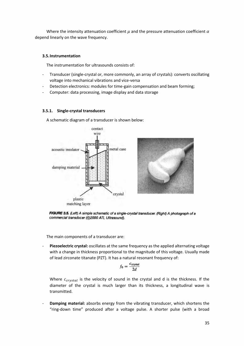
3.5.1. Single-crystal transducers

A schematic diagram of a transducer is shown below:

The main components of a transducer are:

- Piezoelectric crystal: oscillates at the same frequency as the applied alternating voltage

with a change in thickness proportional to the magnitude of this voltage. Usually made

of lead zirconate titanate (PZT). It has a natural resonant frequency of:

Where 𝑐𝑐𝑟𝑦𝑠𝑡𝑎𝑙 is the velocity of sound in the crystal and d is the thickness. If the

diameter of the crystal is much larger than its thickness, a longitudinal wave is

transmitted.

- Damping material: absorbs energy from the vibrating transducer, which shortens the

“ring-down time” produced after a voltage pulse. A shorter pulse (with a broad

36

bandwidth – BW – in the frequency domain) gives a better spatial resolution. It is often

specified the quality factor Q which, in a well damped material, is between 1 and 2.

Since the acoustic impedance of PZT is about 15 times that of skin, there is a huge amount

of energy reflected. Thus, a layer of material with an acoustic impedance 𝑍𝑀𝐿 is placed to

maximize energy transmission:

3.5.1.1. The beam geometry of a single transducer

Considering a plane-piston (flat face) transducer, made up of a large number of point

sources, the total pressure wave emitted is the superposition of the spherical waves emitted by

these point sources:

37

The near-field boundary (NFB) corresponds to the last maximum and separates the near-

field (where the wavefront if not well defined), or Fresnel zone, from the far-field, or Fraunhofer

zone (where the wavefront is well approximated as planar):

Where a is the diameter of the transducer and 𝜆 is the wavelength of the ultrasound.

Beyond this point, the beam diverges and its intensity decreases smoothly. In addition to

the main beam, side lobes may be present due to the transducer acting as a diffraction grating,

which is undesirable since they remove energy from the main beam and can introduce artifacts.

The greater the ratio wavelength/transducer diameter, the fewer the number of side lobes but

the closer the NFB lies to the face of the transducer.

3.5.1.2. Lateral resolution and depth of focus

In the far-field region, the lateral beamwidth can be well approximated by a Gaussian

function, which has a FWHM:

Where 𝜎 is the standard deviation.

Since the diameter of the single-crystal is typically between 1 and 5 cm, the lateral

resolution is usually very poor and a concave lens is used to focus the beam. Lowering the lens

curvature (R) lowers the focal distance F (distance from the face of the transducer at which the

lateral beam width is narrowest). The plane perpendicular to the beam axis at F distance is called

focal plane.

38

For a spherical focusing lens, the FWHM at the focal point is given by

Therefore, decreasing the lens curvature (R) and increasing the diameter of the crystal (a)

improves lateral resolution. The wavelength (𝜆) dependence arises from the appearance of side

lobes as discussed previously.

However, there is a tradeoff: the better the lateral resolution (small FWHM), the lower

the depth of focus as the beam diverges much more at locations away from the focal plane.

3.5.1.3. Axial resolution

Axial resolution is defined as the closest separation, in the direction of the propagating

wave, of two scatterers that result in two backscattered signals. This distance can be expressed

as:

Where PD is the pulse duration. Therefore, axial resolution can be improved by reducing

PD (either by using a higher frequency ultrasound – which also increases attenuation – or

improving the transducer damping).

39

3.5.2. Transducer arrays

There are several problems regarding single crystal transducers:

- Require manual or mechanical steering of the beam;

- Tradeoff between lateral resolution and DOF

- Large distance between the face of the transducer and the NFB

One way of avoiding these problems is to use an array of small piezoelectric crystals. There are

three types of arrays:

3.5.2.1. Linear sequential arrays

A linear sequential array consist of a large number (64-512) of rectangular piezoelectric

crystals, each having a width of the order of the ultrasound wavelength. The width of the

ultrasound is determined by the number of elements that are excited simultaneously. A planar

wavefront is produced by exciting a number of elements (3 for example), which corresponds to

the first line. The process is repeated for the adjacent set (2nd, 3rd and 4th elements), displacing

laterally the focus point, and so on. Additional lines can be acquired by performing again the

same process but with an even number of elements (4 for example).

It is particularly used when a large FOV is required close to the surface of the array.

3.5.2.2. Linear phased arrays

The layout of a linear phased array is very similar to that of a linear sequential array, but

operates in a different way. A much larger number of elements is excited for each line with the

voltage pulses exciting each one being delayed in time in order to produce a curved wavefront

similar to that produced by a focused single crystal transducer. The elements are smaller than

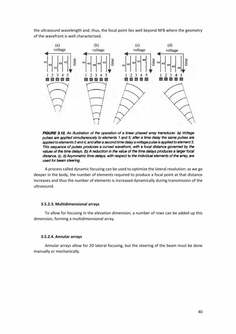
40

the ultrasound wavelength and, thus, the focal point lies well beyond NFB where the geometry

of the wavefront is well characterized.

A process called dynamic focusing can be used to optimize the lateral resolution: as we go

deeper in the body, the number of elements required to produce a focal point at that distance

increases and thus the number of elements is increased dynamically during transmission of the

ultrasound.

3.5.2.3. Multidimensional arrays

To allow for focusing in the elevation dimension, a number of rows can be added up this

dimension, forming a multidimensional array.

3.5.2.4. Annular arrays

Annular arrays allow for 2D lateral focusing, but the steering of the beam must be done

manually or mechanically.

41

3.5.3. Beam forming and time-gain compensation

Time-gate compensation (TGC): signal amplification is dependent on the time that the

signal takes to reach the transducer. Signals arising from structures close to the transducer

(faster to arrive) are amplified by a smaller factor than those from greater depths (which

suffered more attenuation). Various linear or nonlinear functions can be used and adjusted

online by the operator.

3.6. Diagnostic scanning modes

There are three basic modes of diagnostic anatomical imaging: A-mode, M-mode and B-

mode. Recent technical advances include the use of compound and 3D imaging.

3.6.1. A-mode, M-mode and B-mode scans

Amplitude (A)-mode: refers to the acquisition of a 1D scan, that is, a plot of the amplitude

of the backscattered echo versus the time after transmission of the ultrasound pulse. Used for

measuring distances for example in ophthalmology (assuming constant velocity of the sound).

Motion (M)-mode: consists of a series of A-mode scans to detect motion of a moving

structure. The brightness of the displayed signal is proportional to the amplitude of the

backscattered echo.

42

Brightness (B)-mode: produces a 2D image through a cross section of tissue. Each line in

the image consists of an A-mode scan, with the brightness of the signal being proportional to

the amplitude of the backscattered echo. Both stationary and moving structures can be scanned.

3.6.2. Three-dimensional imaging

In 3D imaging, ultrasound waves are sent at different angles and the returning echoes are

processed to reconstruct a 3D image. There are two main approaches:

- Using a 2D US probe for acquiring images by manually moving the probe in a direction

perpendicular to the plane of each B-mode scan;

- Using a dedicated 3D US probe: a 2D array acquires 3D volumes directly.

It allows, for example, better estimation of tumor or cardiac valves dimensions and

detection of fetal malformations.

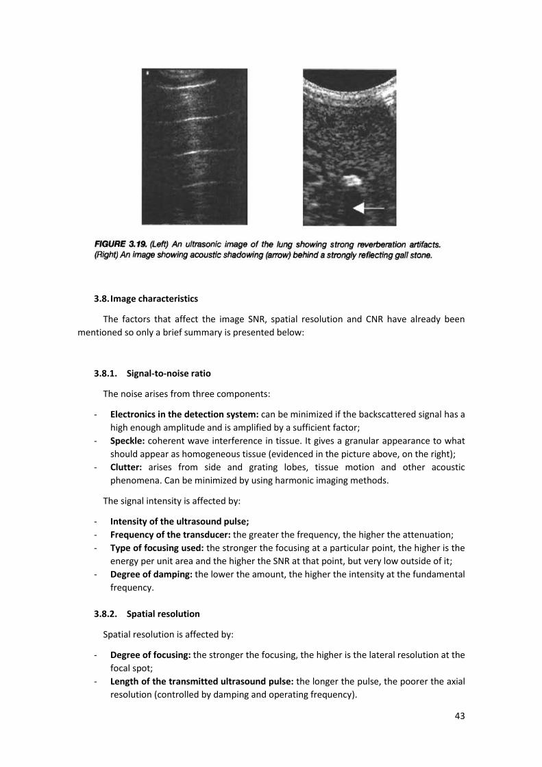
3.7. Artifacts in ultrasonic imaging

Artifacts can result from a number of different effects:

- Reverberations: occur if there is a very strong reflector (bone or air) close to the

transducer surface. Appear as a series of repeated lines;

- Acoustic shadowing: occur if either a very strong reflector (gas/tissue boundary) or

highly attenuating medium shadows a deeper-lying organ. Appears as a dark area or

“hole”;

- Acoustic enhancement: opposite effect of acoustic shadowing. Occurs if region of low

attenuation is present, making the areas appearing behind with higher than expected

intensity. Useful for differentiating fluid-filled cysts from solid masses;

- Refraction: occur when the signal is refracted between two tissues with different

characteristic acoustic impedances (these can result in 20º deviations).

43

3.8. Image characteristics

The factors that affect the image SNR, spatial resolution and CNR have already been

mentioned so only a brief summary is presented below:

3.8.1. Signal-to-noise ratio

The noise arises from three components:

- Electronics in the detection system: can be minimized if the backscattered signal has a

high enough amplitude and is amplified by a sufficient factor;

- Speckle: coherent wave interference in tissue. It gives a granular appearance to what

should appear as homogeneous tissue (evidenced in the picture above, on the right);

- Clutter: arises from side and grating lobes, tissue motion and other acoustic

phenomena. Can be minimized by using harmonic imaging methods.

The signal intensity is affected by:

- Intensity of the ultrasound pulse;

- Frequency of the transducer: the greater the frequency, the higher the attenuation;

- Type of focusing used: the stronger the focusing at a particular point, the higher is the

energy per unit area and the higher the SNR at that point, but very low outside of it;

- Degree of damping: the lower the amount, the higher the intensity at the fundamental

frequency.

3.8.2. Spatial resolution

Spatial resolution is affected by:

- Degree of focusing: the stronger the focusing, the higher is the lateral resolution at the

focal spot;

- Length of the transmitted ultrasound pulse: the longer the pulse, the poorer the axial

resolution (controlled by damping and operating frequency).

44

3.8.3. Contrast-to-noise ratio

Affected by the same factors as SNR. It can be greatly improved by using contrast agents

and pulse inversion techniques, discussed in the next sections.

3.9. Compound Imaging

Also called sonoCT, it consists in acquiring multiple coplanar B-mode scans and combining

them into a single image. Although it presents blurring due to movement across multiple

acquisitions, it has the following advantages:

- Improved SNR (especially in the center, where the lines overlap)

- Reduced speckle and clutter

- Reduced acoustic shadowing

3.10. Blood velocity measurements using ultrasound

Two techniques are used to estimate blood velocity:

- Doppler shift based techniques (used in either continuous – CW – , pulsed or duplex

modes);

- Time-domain signal correlation techniques.

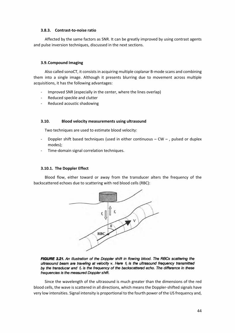
3.10.1. The Doppler Effect

Blood flow, either toward or away from the transducer alters the frequency of the

backscattered echoes due to scattering with red blood cells (RBC):

Since the wavelength of the ultrasound is much greater than the dimensions of the red

blood cells, the wave is scattered in all directions, which means the Doppler-shifted signals have

very low intensities. Signal intensity is proportional to the fourth power of the US frequency and,

45

thus, higher operating frequencies are used (however, maximum measuring depth decreases

with higher frequencies because of the beam attenuation).

The overall Doppler shift ∆𝑓 is given by:

3.10.2. Continuous wave Doppler measurements

CW Doppler uses a continuous pulse transmitted by one transducer and the backscattered

signal is detected by the second one, with the region of overlap of the sensitive regions of the

transducers defining the area in which blood flow is detected (it is often large and the existence

of more than one blood vessel can lead to misinterpretations). It is used when there is no need

to localize exactly the source of Doppler shifts. Its advantages are:

- No maximum depth limitation;

- No maximum measurable velocity limitation.

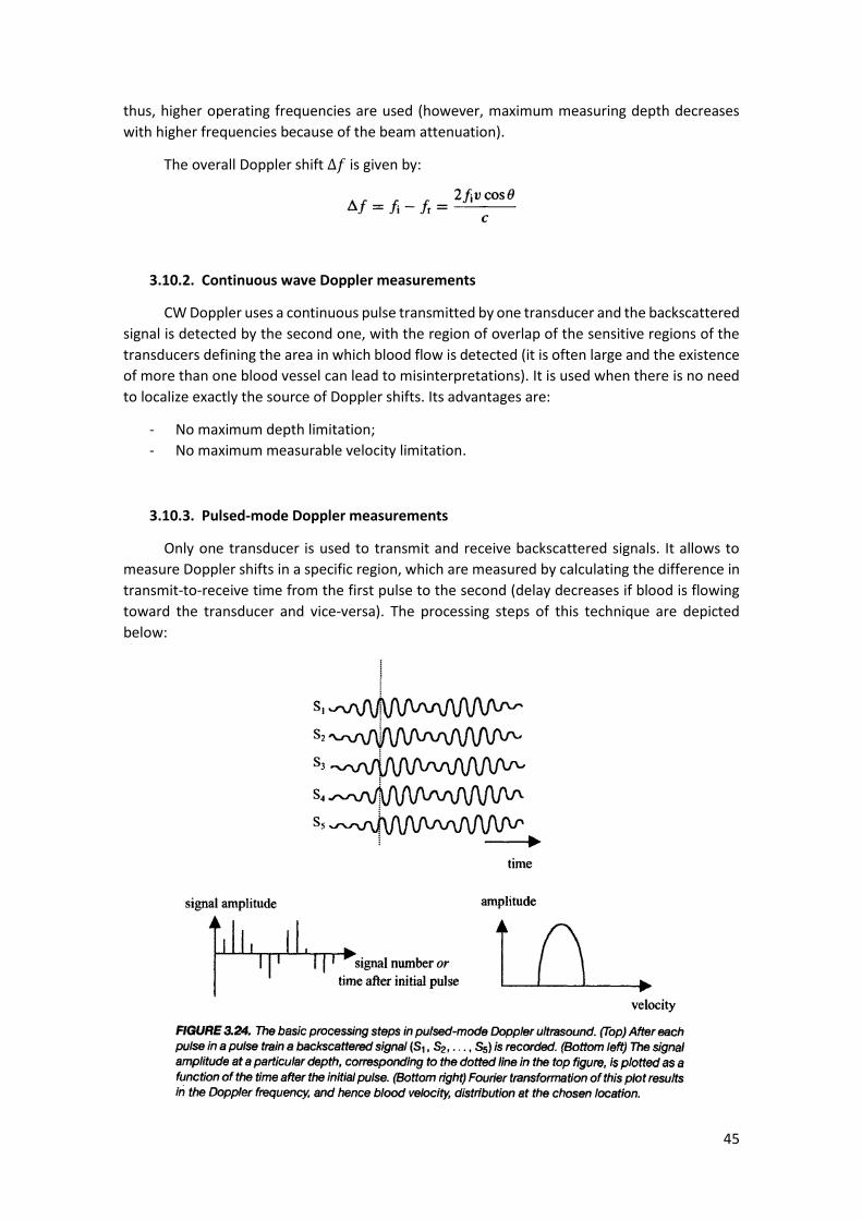
3.10.3. Pulsed-mode Doppler measurements

Only one transducer is used to transmit and receive backscattered signals. It allows to

measure Doppler shifts in a specific region, which are measured by calculating the difference in

transmit-to-receive time from the first pulse to the second (delay decreases if blood is flowing

toward the transducer and vice-versa). The processing steps of this technique are depicted

below:

46

Contrary to CW Doppler, there is a limit to the highest velocity 𝑣𝑚𝑎𝑥which can be

measured imposed by the Nyquist theorem (sampling frequency – in this case, the pulse

repetition rate PRR – must be at least twice the measured frequency). It is given by:

It is also limited to a maximum depth 𝑑𝑚𝑎𝑥:

𝑑𝑚𝑎𝑥 =𝑐

2𝑃𝑅𝑅

3.10.4. Color Doppler/B-mode Duplex Imaging

Duplex imaging consists in interlacing Doppler flow measurements with B-mode imaging

in order to impose the flow maps onto high-resolution anatomical images. Only the mean value

of the velocity and not the full velocity distribution is determined. The mean velocity, its sign

and its variance are represented by the hue, saturation and luminance respectively (red and blue

represents flow towards and away from the transducer, respectively).

When a vessel lies parallel to the face of the transducer array, directly below the center

of the transducer array there is a signal void, which can be solved by using power Doppler mode.

It consists in integrating the area under the frequency vs amplitude plot, allowing to:

- Remove angle dependence (power depends only on the number of RBC scatters);

- Reduce aliasing artifacts at high flow rates.

The main disadvantage of Doppler power is the loss of directional information.

3.11. Ultrasound contrast agents, harmonic imaging and pulse inversion techniques

Contrast agents are used to increase the intensity of backscattered signals and consist of

gas-filled microspheres or microbubbles injected into the bloodstream. They act by two

mechanisms:

- Large increase of the difference in acoustic properties (higher compressibility and lower

density) between gas-filled particles and the surroundings;

- Resonance: gas-filled microspheres expand and contract when the US travels through

them, acting as harmonic oscillators.

These mechanisms results in a much larger effective scattering cross section.

Harmonic Imaging: the backscattered signal consists of a fundamental frequency and its

harmonics. Although these harmonics have lower intensities, they can have higher SNR because

of the very low contributions from clutter and tissue motion. The most common implementation

uses the second harmonic using a pulse inversion technique, which combines two scans. In the

first scan, both the returning fundamental and its harmonic are stored. In the second scan, the

fundamental signal is inverted, but the harmonic has the same phase. Summation of both scans

thus results in the elimination of the fundamental component.

47

4. Magnetic Resonance Imaging

4.1. General principles of Magnetic Resonance Imaging

Magnetic Resonance Imaging (MRI) – nonionizing technique with full 3D capabilities,

excellent soft-tissue contrast and high spatial resolution (~1mm), although expensive and

subject to patient motion due to high scanning times (typically 3-10 mins).

Brief description of the technique – MRI signal arises from protons in the body (mainly

water), which act as small magnets. After the patient is placed inside the scanner, a strong

magnet causes the protons to precess either in a parallel or antiparallel configuration regarding

the direction of the static magnetic field. The frequency of precession is proportional to the

strength of the field. Application of a weak radiofrequency (RF) field causes protons to precess

coherently and the sum of their number is detected as an induced voltage in a tuned detector

coil. Spatial information is encoded into the image using magnetic field gradients (one in each

direction). These gradients cause variations in the magnetic field, which, in turn, causes the

precessional frequencies to vary depending on their spatial location. Frequency and phase is

measured by the RF coil and the signal is then digitized. Finally, an inverse 2D Fourier transform

is performed to convert the signal into the spatial domain.

4.2. Nuclear magnetism

MRI arises from the interaction between the magnetic field and the hydrogen nuclei,

which can be described from a quantum mechanical or classical approach.

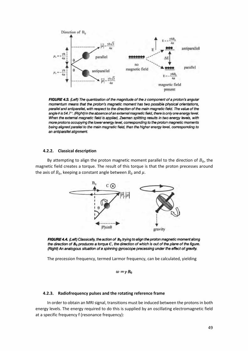
4.2.1. Quantum mechanical description

The spin of a proton can be viewed as a rotation around an internal axis, giving the proton

a certain angular momentum P. Since a proton is a charged particle, it gives the proton a

magnetic moment 𝜇, which, in turn, produces a magnetic field. In the absence of an external

magnetic field, the orientation of the individual magnetic moments is random.

48

The magnitude of P is quantized:

For protons, the spin quantum number l is equal to ½, and thus:

The magnetic momentum 𝜇 is related with P by the gyromagnetic ratio 𝛾:

In the presence of a strong magnetic field 𝐵0, the z component (along 𝐵0) of 𝜇 can only

have the values given by:

The nuclear magnetic quantum number 𝑚𝑙 takes values l, l-1,…,-l so, in the case of a

proton, 𝑚𝑙 takes +1/2 and -1/2, yielding:

𝜇𝑧 = ±𝛾ℎ/4𝜋

The magnetic field only interacts with the z component, thus:

The two possible interaction energies correspond to the parallel (negative E) and

antiparallel (positive E) configurations. The energy difference between the 2 levels is given by:

Using the Boltzmann distribution, we find the relative number of nuclei in each

configuration:

The magnitude of the MRI signal is proportional to the difference in populations between

the 2 energy levels:

Where 𝑁𝑠is the total number of protons in the body.

49

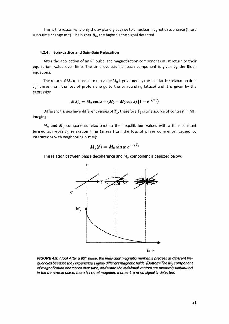
4.2.2. Classical description

By attempting to align the proton magnetic moment parallel to the direction of 𝐵0, the

magnetic field creates a torque. The result of this torque is that the proton precesses around

the axis of 𝐵0, keeping a constant angle between 𝐵0 and 𝜇.

The precession frequency, termed Larmor frequency, can be calculated, yielding

4.2.3. Radiofrequency pulses and the rotating reference frame

In order to obtain an MRI signal, transitions must be induced between the protons in both

energy levels. The energy required to do this is supplied by an oscillating electromagnetic field

at a specific frequency f (resonance frequency):

50

If we refer to the expression in the previous section, we notice that this resonance

frequency is the Larmor frequency.

The electromagnetic energy is provided as a single or series of radiofrequency (RF) pulses.

To analyse the effect of a given sequence of pulses, we will consider the net effect of all of the

protons in the body, thus we define the net magnetization as:

Since the distribution of magnetic momenta in the transverse plane is random, the net

magnetization in x and y directions is zero:

As we will see, a detectable signal can only be produced by 𝑀𝑥 and 𝑀𝑦, so it is necessary

to rotate the net magnetization from z to xy plane by applying a second magnetic field 𝐵1 aligned

along x at the Larmor frequency (much slower than the frequency of 𝐵0). The nuclei are now

said to be phase coherent as all the vectors are pointing in the same direction. The tip angle 𝛼

is defined as the angle through which the net magnetization is rotated. It depends on the

strength and time during which the RF is applied:

To simplify the visualization, we will use a rotating reference frame in which xy plane

rotates around z at the Larmor frequency:

The signal is detected by an RF coil in the form of a voltage E across the ends of the coil

loop, created by the change of the magnetic flux (Faraday’s law):

51

This is the reason why only the xy plane gives rise to a nuclear magnetic resonance (there

is no time change in z). The higher 𝐵0, the higher is the signal detected.

4.2.4. Spin-Lattice and Spin-Spin Relaxation

After the application of an RF pulse, the magnetization components must return to their

equilibrium value over time. The time evolution of each component is given by the Bloch

equations.

The return of 𝑀𝑧 to its equilibrium value 𝑀0 is governed by the spin-lattice relaxation time

𝑇1 (arises from the loss of proton energy to the surrounding lattice) and it is given by the

expression:

Different tissues have different values of 𝑇1, therefore 𝑇1 is one source of contrast in MRI

imaging.

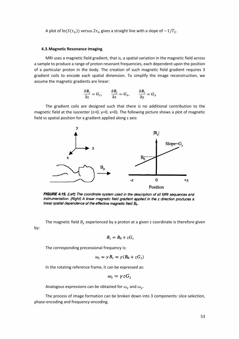
𝑀𝑥 and 𝑀𝑦 components relax back to their equilibrium values with a time constant

termed spin-spin 𝑇2 relaxation time (arises from the loss of phase coherence, caused by

interactions with neighboring nuclei):

The relation between phase decoherence and 𝑀𝑦 component is depicted below:

52

Aside from the nuclei-nuclei interaction, phase decoherence is also affected by spatial

variations of the magnetic field (due to non-uniformities in the magnet design or different

magnetic susceptibilities of different tissues). The overall relaxation of transverse magnetization

is given by 𝑇2∗, a combination of both effects:

Different tissues have different 𝑇2 and, thus, 𝑇2is used as a contrast source as well.

4.2.5. Measurements of 𝑻𝟏 and 𝑻𝟐: inversion recovery and spin-echo sequences

The value of 𝑇1 is measured using an inversion recovery sequence, which consists of a

180º pulse, a variable delay 𝜏 and a 90º pulse, followed immediately by data acquisition. This

sequence is repeated n times, each with a different 𝜏. The detected signal is given by:

A plot of ln (𝑆(𝜏𝑛)) versus 𝜏𝑛 gives a straight line with a slope of −𝑇1.

The measurement of 𝑇2 involves a spin-echo setup, where a 90º is applied, followed by a

variable delay 𝜏, a 180º pulse (in the xy plane), an identical 𝜏 and then the signal acquisition. To

see how the spin-echo sequence works, consider a single proton which, due to spatial

inhomogeneities in the magnetic field, resonates at a frequency Δ𝜔, less than the nominal

Larmor frequency. At 𝜏 after the 90º pulse, the precessing magnetization has accumulated a

phase 𝜙 = Δωτ. By applying the 180º pulse, we convert 𝑀𝑦to −𝑀𝑦 and +𝜙 to −𝜙. During the

second 𝜏 interval, the precessing magnetization accumulates a further phase +𝜙. Thus, at 2𝜏,

the precessing magnetization has 0 phase, which eliminates the 𝑇2+ contribution, yielding 𝑇2

∗ =

𝑇2:

53

A plot of ln (𝑆(𝜏𝑛)) versus 2𝜏𝑛 gives a straight line with a slope of −1/𝑇2.

4.3. Magnetic Resonance Imaging

MRI uses a magnetic field gradient, that is, a spatial variation in the magnetic field across

a sample to produce a range of proton resonant frequencies, each dependent upon the position

of a particular proton in the body. The creation of such magnetic field gradient requires 3

gradient coils to encode each spatial dimension. To simplify the image reconstruction, we

assume the magnetic gradients are linear:

The gradient coils are designed such that there is no additional contribution to the

magnetic field at the isocenter (z=0, y=0, x=0). The following picture shows a plot of magnetic

field vs spatial position for a gradient applied along z axis:

The magnetic field 𝐵𝑧 experienced by a proton at a given z coordinate is therefore given

by:

The corresponding precessional frequency is:

In the rotating reference frame, it can be expressed as:

Analogous expressions can be obtained for 𝜔𝑥 and 𝜔𝑦.

The process of image formation can be broken down into 3 components: slice selection,

phase-encoding and frequency-encoding.

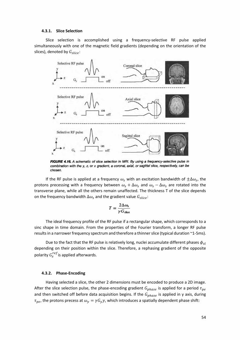
54

4.3.1. Slice Selection

Slice selection is accomplished using a frequency-selective RF pulse applied

simultaneously with one of the magnetic field gradients (depending on the orientation of the

slices), denoted by 𝐺𝑠𝑙𝑖𝑐𝑒:

If the RF pulse is applied at a frequency 𝜔𝑠 with an excitation bandwidth of ±Δ𝜔𝑠, the

protons precessing with a frequency between 𝜔𝑠 + Δ𝜔𝑠 and 𝜔𝑠 − Δ𝜔𝑠 are rotated into the

transverse plane, while all the others remain unaffected. The thickness T of the slice depends

on the frequency bandwidth ∆𝜔𝑠 and the gradient value 𝐺𝑠𝑙𝑖𝑐𝑒:

The ideal frequency profile of the RF pulse if a rectangular shape, which corresponds to a

sinc shape in time domain. From the properties of the Fourier transform, a longer RF pulse

results in a narrower frequency spectrum and therefore a thinner slice (typical duration ~1-5ms).

Due to the fact that the RF pulse is relatively long, nuclei accumulate different phases 𝜙𝑠𝑙

depending on their position within the slice. Therefore, a rephasing gradient of the opposite

polarity 𝐺𝑧𝑟𝑒𝑓

is applied afterwards.

4.3.2. Phase-Encoding

Having selected a slice, the other 2 dimensions must be encoded to produce a 2D image.

After the slice selection pulse, the phase-encoding gradient 𝐺𝑝ℎ𝑎𝑠𝑒 is applied for a period 𝜏𝑝𝑒

and then switched off before data acquisition begins. If the 𝐺𝑝ℎ𝑎𝑠𝑒 is applied in y axis, during

𝜏𝑝𝑒, the protons precess at 𝜔𝑦 = 𝛾𝐺𝑦𝑦, which introduces a spatially dependent phase shift:

55

4.3.3. Frequency-Encoding

The frequency-encoding is encoded by the nuclei precessing at different frequencies

under the influence of a gradient 𝐺𝑓𝑟𝑒𝑞 , which is applied during data acquisition. The time

between successive acquisitions is referred to as dwell time 𝑡𝑑𝑤, being the reciprocal of the

acquisition bandwidth.

A graphical representation of the slice, frequency and phase encoding processes is

depicted below:

4.3.4. The k-Space formalism

To understand how the acquired 𝑁𝑟 × 𝑁𝑝 data matrix is transformed into the final image,

we will look into the k-space formalism. First, we define two variables:

With x and y being the frequency and phase encoding directions respectively. The signal

can then be expressed as:

The 𝑁𝑟 × 𝑁𝑝 acquisition points can be visualized as a 2D data set in k-space. Consider the

𝑁𝑟 points collected when the minimum value of the phase encoding 𝐺𝑦 is applied. Referring to

56

the 𝑘𝑦 expression, all these 𝑁𝑟 have the minimum 𝑘𝑦 value. When the frequency-encoding

gradient is turned on, the first data point collected corresponds to a small positive value of 𝑘𝑥,

the second data point to a slightly more positive value of 𝑘𝑥 and so forth, and so these 𝑁𝑟 points

correspond to the first (bottom) line in k-space. The second line corresponds to the next value

of the phase encoding gradient and so on. The spacing between k-space points is dictated by the

required FOV of the image:

A 2D inverse Fourier transform of the k-space data 𝑆(𝑘𝑥 , 𝑘𝑦) gives an estimation of

𝜌(𝑥, 𝑦), that is, an image corresponding to the spatial variation in proton density. In the previous

example only the positive half of the 𝑘𝑥 was acquired. In full k-space coverage, the SNR and

spatial resolution (determined by the maximum values of 𝑘𝑥 and 𝑘𝑦) would be increased. This

can be achieved by a gradient-echo imaging sequence, which adds a negative gradient 𝐺𝑑𝑒𝑝ℎ𝑎𝑠𝑒

before data acquisition.

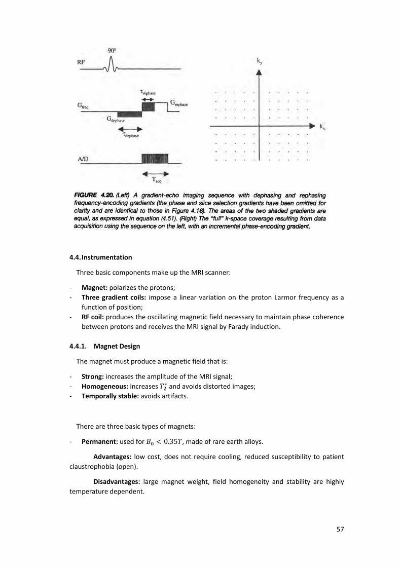
57

4.4. Instrumentation

Three basic components make up the MRI scanner:

- Magnet: polarizes the protons;

- Three gradient coils: impose a linear variation on the proton Larmor frequency as a

function of position;

- RF coil: produces the oscillating magnetic field necessary to maintain phase coherence

between protons and receives the MRI signal by Farady induction.

4.4.1. Magnet Design

The magnet must produce a magnetic field that is:

- Strong: increases the amplitude of the MRI signal;

- Homogeneous: increases 𝑇2∗ and avoids distorted images;

- Temporally stable: avoids artifacts.

There are three basic types of magnets:

- Permanent: used for 𝐵0 < 0.35𝑇, made of rare earth alloys.

Advantages: low cost, does not require cooling, reduced susceptibility to patient

claustrophobia (open).

Disadvantages: large magnet weight, field homogeneity and stability are highly

temperature dependent.

58

- Resistive: used for 𝐵0 < 0.35𝑇, magnetic field strength is proportional to a constant

current passing through a conductor such as copper. Power dissipated as heat is

proportional to the resistance of the conductor and the square of the current.

Disadvantages: requires cooling, maximum magnetic field strength is limited by the

maximum current, homogeneity and stability highly dependent on temperature.

- Superconducting: used for 𝐵0 > 0.35𝑇 (typically 1.5T or 3T). It minimizes the problem

of cooling by using superconductors which have 0 resistance at very low temperatures

and allows stronger magnetic fields to be used. The superconductor is housed in a can

containing liquid helium at 4.2K, surrounded by radiation shields, vacuum vessels and a

liquid nitrogen chamber. Because heat losses are not avoidable, liquid nitrogen and

helium must be replenished on a regular basis. Additional correction and shim coils are

added to correct uniformity of the magnetic field.

4.4.2. Magnetic field gradient coils

Gradient coils have three basic requirements:

- Production of linear gradients over the imaged region: their geometry is optimized to

produce a linear gradient, rather than a uniform field. Since the value of the gradient is

relatively small, chilled water cooling is sufficient. The z coil consists of a “Maxwell pair”

(two separate loops, with current flowing in opposed directions). The x and y coils have

a “saddle coil” arrangement (four arcs each). The gradient strength is proportional to

the number of turns.

- Production of high gradient strengths per unit current: achieved by minimizing

resistance;

- Fast switching times: achieved by minimizing inductance; important to reduce the time

which must be allowed for gradients to stabilize in imaging techniques.

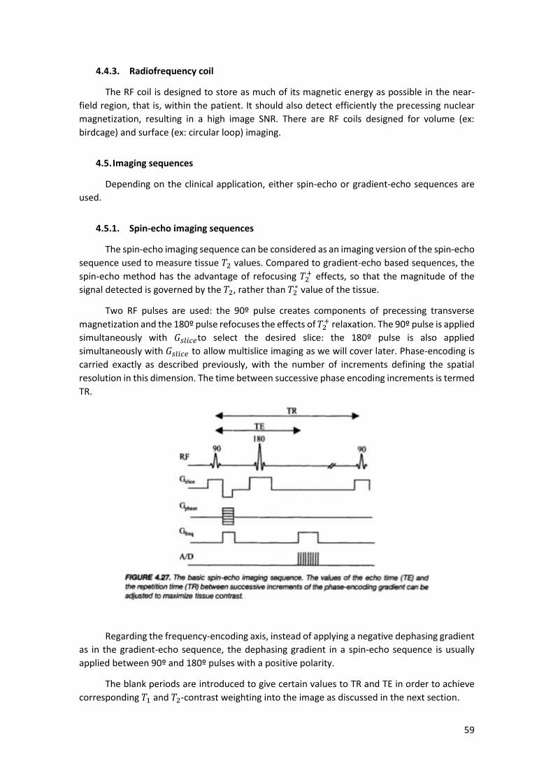
59

4.4.3. Radiofrequency coil

The RF coil is designed to store as much of its magnetic energy as possible in the near-

field region, that is, within the patient. It should also detect efficiently the precessing nuclear

magnetization, resulting in a high image SNR. There are RF coils designed for volume (ex:

birdcage) and surface (ex: circular loop) imaging.

4.5. Imaging sequences

Depending on the clinical application, either spin-echo or gradient-echo sequences are

used.

4.5.1. Spin-echo imaging sequences

The spin-echo imaging sequence can be considered as an imaging version of the spin-echo

sequence used to measure tissue 𝑇2 values. Compared to gradient-echo based sequences, the

spin-echo method has the advantage of refocusing 𝑇2+ effects, so that the magnitude of the

signal detected is governed by the 𝑇2, rather than 𝑇2∗ value of the tissue.

Two RF pulses are used: the 90º pulse creates components of precessing transverse

magnetization and the 180º pulse refocuses the effects of 𝑇2+ relaxation. The 90º pulse is applied

simultaneously with 𝐺𝑠𝑙𝑖𝑐𝑒to select the desired slice: the 180º pulse is also applied

simultaneously with 𝐺𝑠𝑙𝑖𝑐𝑒 to allow multislice imaging as we will cover later. Phase-encoding is

carried exactly as described previously, with the number of increments defining the spatial

resolution in this dimension. The time between successive phase encoding increments is termed

TR.

Regarding the frequency-encoding axis, instead of applying a negative dephasing gradient

as in the gradient-echo sequence, the dephasing gradient in a spin-echo sequence is usually

applied between 90º and 180º pulses with a positive polarity.

The blank periods are introduced to give certain values to TR and TE in order to achieve

corresponding 𝑇1 and 𝑇2-contrast weighting into the image as discussed in the next section.

60

4.5.2. 𝑻𝟏 and 𝑻𝟐-weighted imaging sequences

The intensity of an axial image acquired using a spin-echo sequence is given by:

The term 1 − 𝑒−𝑇𝑅/𝑇1 determines the 𝑇1 weighting of the sequence. If the TR value (which

can be set by the operator) is set to a value much greater than 𝑇1, then the image has no 𝑇1-

weighting as the term 1 − 𝑒−𝑇𝑅/𝑇1 is very similar for all tissues. If the TR value is set closer to

the tissue 𝑇1 then the image becomes more 𝑇1-weighted. As the TR values becomes smaller, the

SNR decreases, although the total imaging time (𝑁𝑝 × 𝑇𝑅) also decreases (the goal is to decrease

imaging time while maintaining sufficient SNR for accurate diagnosis).

The same considerations apply to the term 𝑒−𝑇𝐸/𝑇2, which determines the degree of 𝑇2-

weighting: if the value of TE is set much shorter than the tissue 𝑇2, then no 𝑇2 contrast is present;

if the value of TE is too long, then the contrast is high, but the SNR is low (the goal is to have the

highest CNR).

4.5.2.1. Which physical properties influence 𝑻𝟏 and 𝑻𝟐?

The mechanism of 𝑇1 relaxation involves the protons losing their excess energy via

interactions with oscillating magnetic fields, produced by nuclei in surrounding molecules as

they execute random Brownian motion. When these randomly fluctuating magnetic fields have

a component at the Larmor frequency, they can stimulate transitions between the antiparallel

and parallel states, and thereby cause the 𝑀𝑧 component to return to 𝑀0. Thus, slowly moving

molecules (low frequency) in a viscous media have higher contributions to 𝑇1 at low magnetic

field strengths, while rapidly moving molecules (high frequency) in mobile liquids produce

fluctuating magnetic fields over a wide frequency range. The spectral density 𝐽(𝜔) is a measure

of the number of nuclei capable of producing magnetic fields at the Larmor frequency, thus the

greater 𝐽(𝜔), the shorter is 𝑇1:

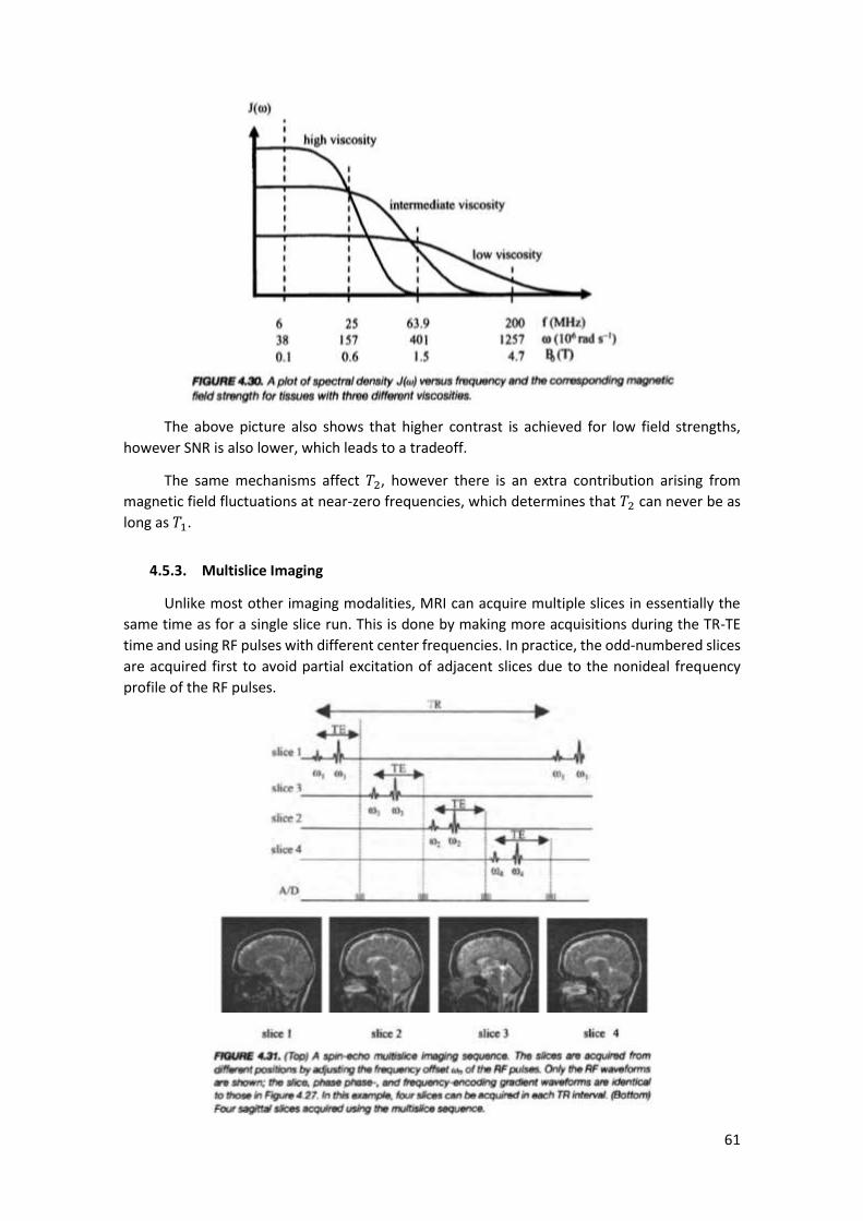
61

The above picture also shows that higher contrast is achieved for low field strengths,

however SNR is also lower, which leads to a tradeoff.

The same mechanisms affect 𝑇2, however there is an extra contribution arising from

magnetic field fluctuations at near-zero frequencies, which determines that 𝑇2 can never be as

long as 𝑇1.

4.5.3. Multislice Imaging

Unlike most other imaging modalities, MRI can acquire multiple slices in essentially the

same time as for a single slice run. This is done by making more acquisitions during the TR-TE

time and using RF pulses with different center frequencies. In practice, the odd-numbered slices

are acquired first to avoid partial excitation of adjacent slices due to the nonideal frequency

profile of the RF pulses.

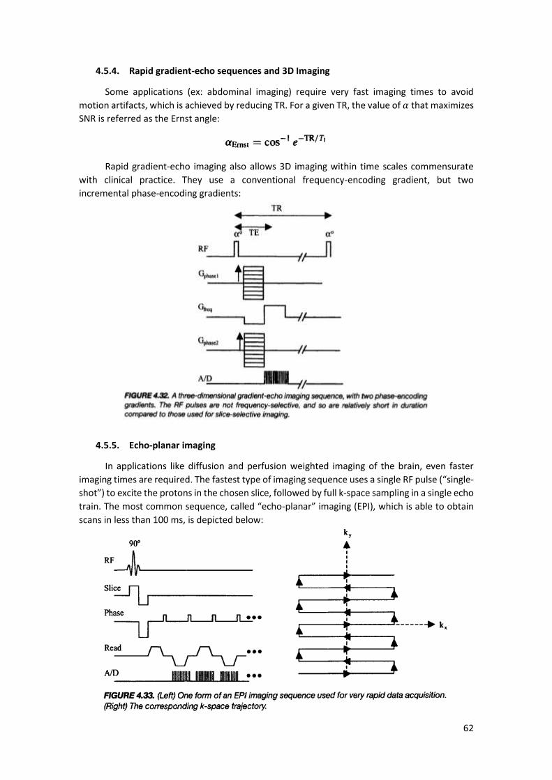
62

4.5.4. Rapid gradient-echo sequences and 3D Imaging

Some applications (ex: abdominal imaging) require very fast imaging times to avoid

motion artifacts, which is achieved by reducing TR. For a given TR, the value of 𝛼 that maximizes

SNR is referred as the Ernst angle:

Rapid gradient-echo imaging also allows 3D imaging within time scales commensurate

with clinical practice. They use a conventional frequency-encoding gradient, but two

incremental phase-encoding gradients:

4.5.5. Echo-planar imaging

In applications like diffusion and perfusion weighted imaging of the brain, even faster

imaging times are required. The fastest type of imaging sequence uses a single RF pulse (“single-

shot”) to excite the protons in the chosen slice, followed by full k-space sampling in a single echo

train. The most common sequence, called “echo-planar” imaging (EPI), which is able to obtain

scans in less than 100 ms, is depicted below:

63

This sequence can introduce an unacceptable level of image blurring due to the broad

PSF, which arises from 𝑇2∗ relaxation during the sequence. To overcome this, a segmented mode

can be used, where, for instance, only every fourth data point is acquired and the process is

repeated 4 times.

4.5.6. Spiral imaging

Instead of a rectangular k-space trajectory, “spiral imaging” uses a spiral trajectory, which

presents two basic advantages:

- Low spatial frequencies are sampled more densely, because the spiral is tightest close

to the origin of the k-space axis. This results in higher SNR and compensation for patient

motion;

- The gradient “slew rate” (rate at which strength is changed) is slower.

Prior to the 2D inverse Fourier transform, an interpolation onto a rectangular grid must

be performed. A segmented mode is also commonly used.

4.6. Image characteristics

The tradeoffs and factors that affect SNR, spatial resolution and CNR are discussed below.

4.6.1. Signal-to-noise ratio

The main factors affecting SNR are:

- Magnetic field 𝐵0 strength: improves nuclear polarization and voltage measured by

Faraday induction (↑)

- RF coil sensitivity: defined as the 𝐵1 field produced per unit current (↑)

- Noise contributions from the RF coil and the sample: random voltage fluctuations (↓)

- Number of phase encoding steps 𝑁𝑝(↓)

- Number of frequency encoding steps 𝑁𝑟(↓)

- Slice thickness (↑)

64

4.6.2. Spatial resolution

The image PSF is different in each spatial dimension. In the slice-select direction, the PSF

is simply related to the RF pulse frequency profile (slice thickness). In the frequency and phase

encoding directions, three factors affect the PSF:

- Digital resolution: defined as FOV/Number of data points acquired.

- Data truncation: because only a finite number of frequency and phase encoding data

points are taken, the data are effectively truncated and the corresponding PSF is a sinc

function. The width of the sinc function in each dimension is inversely proportional to

the number of data points acquired;

- 𝑻𝟐∗ relaxation time: the exponential decay corresponds to a Lorentzian PSF, which

FWHM decreases when 𝑇2∗ increases:

4.6.3. Contrast-to-noise ratio

CNR is essentially dependent on the difference between the relaxation times and proton

density and the values of TR and TE. There is also a dependence on the strength of 𝐵0 since 𝑇1-

weighted contrast is higher for lower 𝐵0. Since CNR between two tissues depends on the

respective SNRs, CNR is also affected by the factors listed for SNR.

4.7. MRI contrast agents

In certain situations such as the detection of very small lesions, where the signal from the

lesion is effectively averaged with that of healthy tissue, the CNR can be very low. In this case,

one of two basic types of MRI contrast agents can be used:

- Paramagnetic agents: shorten 𝑇1; tissues on which it accumulate appear bright;

- Superparamagnetic (or ferromagnetic): shorten 𝑇2 and 𝑇2∗, accumulate primarily in

healthy tissues.

4.7.1. Paramagnetic agents

Paramagnetic agents are based on metal ions such as gadolinium that have a large number

of unpaired electrons (with high magnetic moments). The interactions between the unpaired

electrons and the water molecules cause the proton 𝑇1 to be shortened, with the effect being

quantified by the relaxivity of the agent:

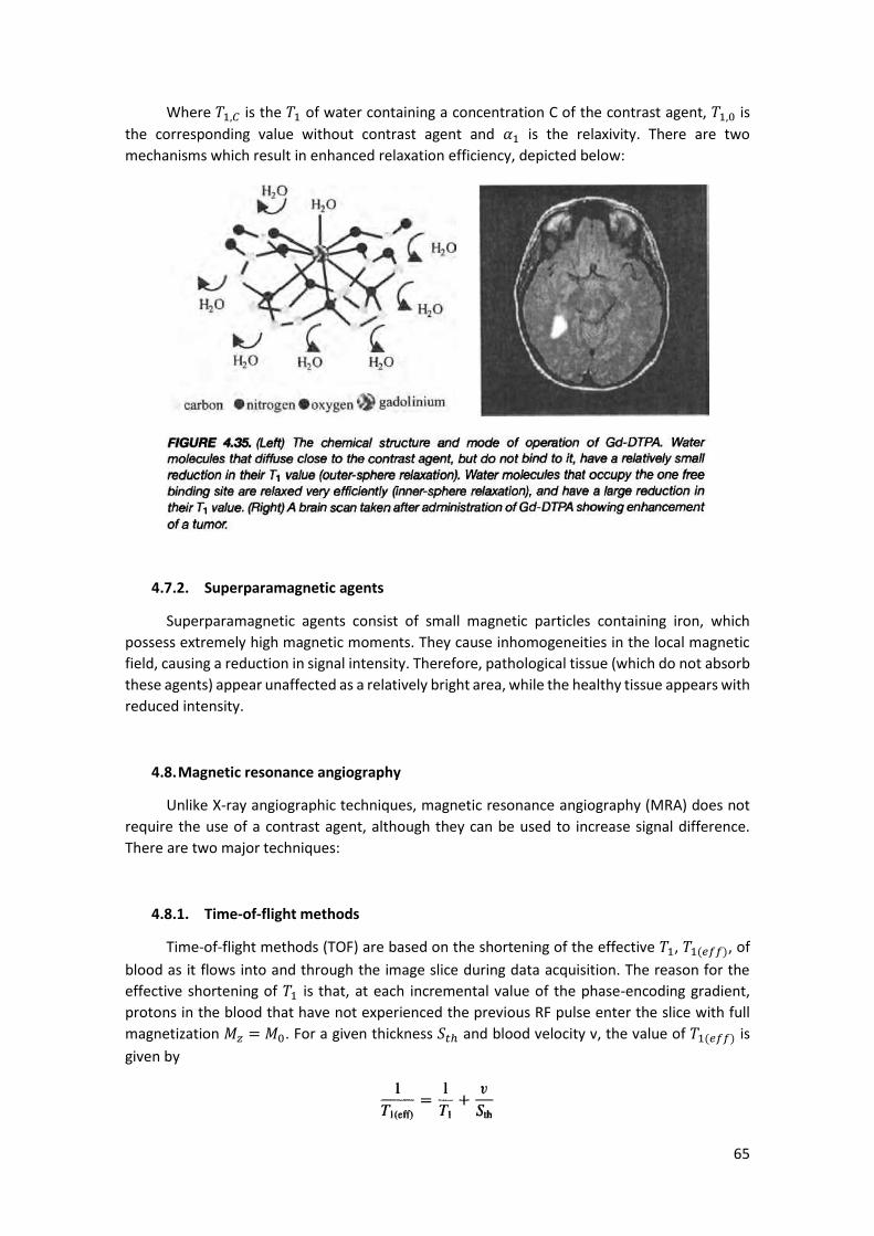
65

Where 𝑇1,𝐶 is the 𝑇1 of water containing a concentration C of the contrast agent, 𝑇1,0 is

the corresponding value without contrast agent and 𝛼1 is the relaxivity. There are two

mechanisms which result in enhanced relaxation efficiency, depicted below:

4.7.2. Superparamagnetic agents

Superparamagnetic agents consist of small magnetic particles containing iron, which

possess extremely high magnetic moments. They cause inhomogeneities in the local magnetic

field, causing a reduction in signal intensity. Therefore, pathological tissue (which do not absorb

these agents) appear unaffected as a relatively bright area, while the healthy tissue appears with

reduced intensity.

4.8. Magnetic resonance angiography

Unlike X-ray angiographic techniques, magnetic resonance angiography (MRA) does not

require the use of a contrast agent, although they can be used to increase signal difference.

There are two major techniques:

4.8.1. Time-of-flight methods

Time-of-flight methods (TOF) are based on the shortening of the effective 𝑇1, 𝑇1(𝑒𝑓𝑓), of

blood as it flows into and through the image slice during data acquisition. The reason for the

effective shortening of 𝑇1 is that, at each incremental value of the phase-encoding gradient,

protons in the blood that have not experienced the previous RF pulse enter the slice with full

magnetization 𝑀𝑧 = 𝑀0. For a given thickness 𝑆𝑡ℎ and blood velocity v, the value of 𝑇1(𝑒𝑓𝑓) is

given by

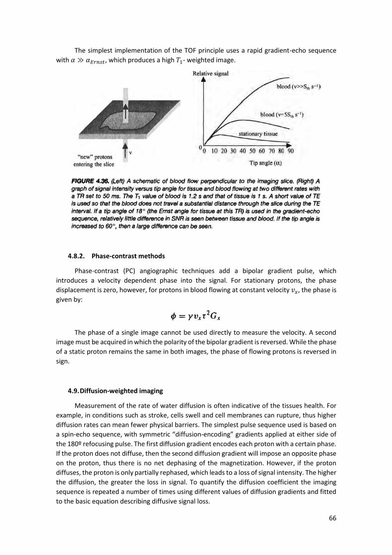
66

The simplest implementation of the TOF principle uses a rapid gradient-echo sequence

with 𝛼 ≫ 𝛼𝐸𝑟𝑛𝑠𝑡, which produces a high 𝑇1- weighted image.

4.8.2. Phase-contrast methods

Phase-contrast (PC) angiographic techniques add a bipolar gradient pulse, which

introduces a velocity dependent phase into the signal. For stationary protons, the phase

displacement is zero, however, for protons in blood flowing at constant velocity 𝑣𝑥, the phase is

given by:

The phase of a single image cannot be used directly to measure the velocity. A second

image must be acquired in which the polarity of the bipolar gradient is reversed. While the phase

of a static proton remains the same in both images, the phase of flowing protons is reversed in

sign.

4.9. Diffusion-weighted imaging

Measurement of the rate of water diffusion is often indicative of the tissues health. For

example, in conditions such as stroke, cells swell and cell membranes can rupture, thus higher

diffusion rates can mean fewer physical barriers. The simplest pulse sequence used is based on

a spin-echo sequence, with symmetric “diffusion-encoding” gradients applied at either side of

the 180º refocusing pulse. The first diffusion gradient encodes each proton with a certain phase.

If the proton does not diffuse, then the second diffusion gradient will impose an opposite phase

on the proton, thus there is no net dephasing of the magnetization. However, if the proton

diffuses, the proton is only partially rephased, which leads to a loss of signal intensity. The higher

the diffusion, the greater the loss in signal. To quantify the diffusion coefficient the imaging

sequence is repeated a number of times using different values of diffusion gradients and fitted

to the basic equation describing diffusive signal loss.

67

4.10. Functional MRI

fMRI makes use of the sensitivity of the MRI signal intensity to the level of oxygen in the

blood in the brain (oxygen-level-dependent – BOLD – effect) to determine which areas of the

brain are involved in specific cognitive tasks. In gray matter in the brain, a modest increase in

the cerebral metabolic rate of oxygen (MCRO2) and of glucose occurs in areas involved in neural

activation, which leads to the release of vasodilatory compounds and increase of blood flow in

the capillary bed. The rate of delivery of oxygen increases, but to a much lesser extent than the

increase in blood flow, which leads to an oxygenation of blood. This, in turn, increases the level

of oxyhemoglobin and decreases the level of deoxyhemoglobin. The decrease in

deoxyhemoglobin reduces the local magnetic field gradients between the blood in the capillary

bed and tissue, which leads to an increase of 𝑇2 and 𝑇2∗ in areas of the brain associated with

neural activation.

The most common sequence used is the multislice EPI because it is fast enough to obtain

whole brain coverage in a few seconds. The changes in image intensity in activated areas are

very small, thus the experiments are repeated a number of times and the data is subjected to

statistical analysis and filtering.

The changing in MRI signal intensity at sites associated with neuronal activation has three

components:

- Small signal decrease immediately after the onset of the stimulation, which corresponds

to the total deoxyhemoglobin increasing for the first 3 s due to an initial increase in

oxygen extraction before the increase in blood flow;

- Increase in signal intensity, which reaches a maximum at about 7 s after the onset of the

stimulus (hemodynamic response time);

- Signal undershoot which can last up to 1 min and corresponds to the blood volume in

the venules.

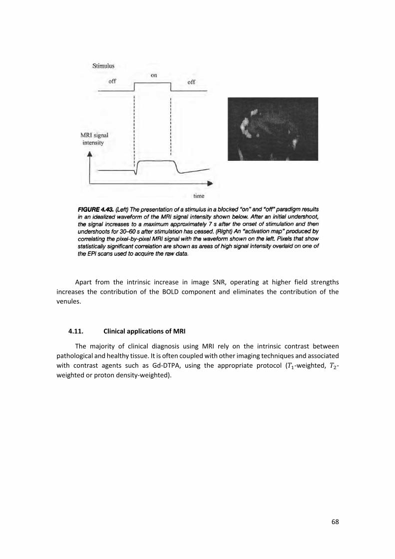
68

Apart from the intrinsic increase in image SNR, operating at higher field strengths

increases the contribution of the BOLD component and eliminates the contribution of the

venules.

4.11. Clinical applications of MRI

The majority of clinical diagnosis using MRI rely on the intrinsic contrast between

pathological and healthy tissue. It is often coupled with other imaging techniques and associated

with contrast agents such as Gd-DTPA, using the appropriate protocol (𝑇1-weighted, 𝑇2-

weighted or proton density-weighted).