Multiphysics Model of Metal Solidification on the Continuum Level

Seid Korica, Lance C. Hibbelerb, Rui Liub, Brian G. Thomasb

a National Center for Supercomputing Applications, University of Illinois, Urbana, IL, 61801

b Department of Mechanical Science and Engineering, University of Illinois, Urbana, IL, 61801

Abstract

Separate three-dimensional (3-D) models of thermo-mechanical behavior of the solidifying shell,

turbulent fluid flow in the liquid pool, and thermal distortion of the mold are combined to create an

accurate multiphysics model of metal solidification at the continuum level. The new system is applied to

simulate continuous casting of steel in a commercial beam-blank caster with complex geometry. A

transient coupled elastic-viscoplastic model (Koric and Thomas, 2006) computes temperature and stress

in a transverse slice through the mushy and solid regions of the solidifying metal. This Lagrangian model

features an efficient numerical procedure to integrate the constitutive equations of the delta-ferrite and

austenite phases of solidifying steel shell using a fixed-grid finite-element approach. The Navier-Stokes

equations are solved in the liquid pool using the standard K-ε turbulent flow model with standard wall

laws at the mushy zone edges that define the domain boundaries. The superheat delivered to the shell is

incorporated into the thermal-mechanical model of the shell using the enhanced latent heat method

(Koric et al., 2010). Temperature and thermal distortion modeling of the complete complex-shaped mold

includes the tapered copper plates, water cooling slots, backing plates, and nonlinear contact between the

different components. Heat transfer across the interfacial gaps between the shell and the mold is fully

coupled with the stress model to include the effect of shell shrinkage and gap formation on lowering the

heat flux. The model is validated by comparison with analytical solutions of benchmark problems of

conduction with phase change (Dantzig and Tucker, 2001), and thermal stress in an unconstrained

solidifying plate (Weiner and Boley, 1963). Finally, results from the complete system compare favorably

with plant measurements of shell thickness.

Keywords: Solidification, Mutiphysics, Thermal-Stress, Fluid Flow, Superheat, Viscoplastic, Turbulence,

Continuous Casting

1. Introduction and Previous Work

Many manufacturing processes, such as foundry casting, continuous casting, and welding, are governed

by multiple coupled phenomena which include turbulent fluid flow, heat transfer, solidification,

distortion, and stress generation. The difficulty of plant experiments under harsh operating conditions

makes computational modeling an important tool in the design and optimization of these processes.

Increased computing power and better numerical methods have enabled researchers to develop better

models of many different aspects of these processes. Coupling together the different models of the

different phenomena to make accurate predictions of the entire real processes remains a challenge.

In early work (Weiner and Boley, 1963) a semi-analytical solution was derived for the thermal stresses

arising during the solidification of a semi-infinite plate. Although that work oversimplifies the complex

physical phenomena of solidification, it has become a useful benchmark problem for the verification of

numerical models. The constitutive models used in previous models of thermal stresses during continuous

casting first adopted simple elastic-plastic laws (Weiner and Boley 1963, Grill et al., 1976) and simple

creep laws (Rammerstrofer et al., 1979, Kristiansson, 1984). With improving computer hardware, more

computationally challenging elastic-viscoplastic models have been used (Zhu 1993, Boehmer et al., 1998,

Li and Thomas, 2004, Risso et al., 2006, Koric and Thomas, 2006). While the Lagrangian description of

this process with a fixed mesh is widely adopted due to its easy implementation, an alternative

mechanical model based on an arbitrary Eulerian-Lagrangian description has been implemented as well

(Risso et al., 2006). To enable fast convergence of the highly-nonlinear constitutive equations that

accompany solidification and high-temperature deformation, a robust local viscoplastic integration

scheme (Zhu, 1993, Li and Thomas 2004) has been implemented (Koric and Thomas, 2006) into the

commercial finite element package ABAQUS (Dassault Corp., 2009) via its user defined material

subroutine UMAT, including special treatment of liquid/mushy zone. This enables realistic

computational modeling of complex solidification processes with ABAQUS (Koric et al., 2009, Hibbeler

et al., 2009).

As the demand for better computer simulations of solidification processes increases, there is a growing

need to include the effects of fluid flow into thermo-mechanical analyses. The multiphysics approach of

simulating all three macroscale phenomena (i.e. fluid flow, solidification heat transfer, and mechanical

distortion) simultaneously has been demonstrated in several previous works,(ref cross, others??) but is

very computationally demanding for realistic problems. Major difficulties stem from the inherently

different coordinate descriptions and numerical techniques used in the separate models for these three

fields. Fluid flow typically is performed on structured Eulerian domains using steady-state control-

volume methods with iterative solution algorithms. Stress analysis typically is performed on unstructured

Lagrangian domains using transient finite-element methods with direct solvers. Many different methods

are used to treat heat transfer with moving solidification front(s).(Voller review??) Further difficulties

arise from the complex geometries, which require large computational meshes.

Lee and coworkers (Lee et al., 2000) showcased multiphysics modeling by coupling a 3-D finite-

difference model of fluid flow with a 2-D transient thermal-stress model to predict solidification, gap

formation, stress, and crack formation in a beam-blank caster. Teskeredzic et al. (Teskeredzic et al.,

2002) used a 2D multiphysics finite-volume method for simultaneous prediction of physical phenomena

during a solid/liquid phase change. Neither prediction was validated with plant measurements. Some

researchers attempted to decouple the thermal-fluid simulation from the stress analysis (Shamsi et al.,

2008, Pokorny et al., 2008) but this neglects the important effects of shrinkage and deformation on heat

transfer, such as that caused by increased pressure or gap formation between the casting and the mold (Ho

and Pehlke, 1985).

Alternatively, the fluid flow simulation can be reasonably decoupled from the thermal-stress analysis if

the liquid pool shape can be estimated a-priori and the mechanical influence of fluid on the solid shell is

modeled with hydrostatic pressure boundary conditions. Doing so is relatively easy for many processes

involving a stable interface shape, such as ledge formation in cryolite electrolysis or the continuous

casting of steel. Such simulations can readily output the “superheat flux” that delivers heat to the

solidification front, such as characterized by the liquidus temperature. Recently Koric et al. (Koric et al.,

2010) has demonstrated that “superheat flux” can be incorporated into a transient simulation of heat

transfer phenomena in the mushy and solid regions by enhancing the latent heat in the mushy zone

without an explicit need to track the solidification front. The procedure has been added into the

commercial package ABAQUS (Dassault Corp., 2009) with a user-defined subroutine UMATHT. In the

present work, this approach is applied to perform a realistic simulation of turbulent fluid flow, heat

transfer, solidification, stress, and mold distortion of a commercial beam-blank caster.

The continuous casting process used here to exemplify multiphysics modeling is used to produce nearly

all of the steel in the world. The process empties ladles of molten steel through a vessel called a tundish,

which stores steel between changes and also helps to clean the metal. The tundish drains into a

bottomless, water-cooled copper mold, which extracts heat from the molten steel and solidifies a shell.

The shell is withdrawn at a rate called the casting speed into a region of water sprays, which complete the

solidification. Slabs are then cut to the desired length and sent for downstream processing, such as

rolling. The molds produce thick or thin slabs, square billets, blooms, rounds, and also near-net-shape

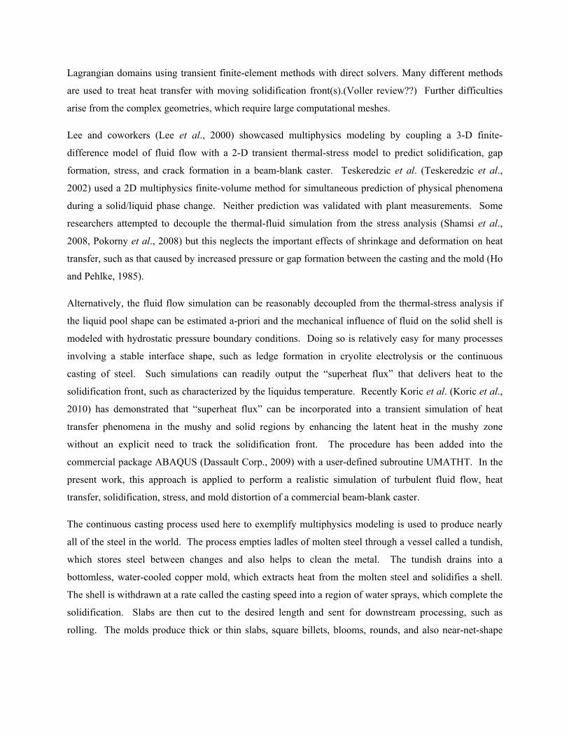
“beam blank” or “dogbone” cross-sections. Fig. 5 shows a cross section of a typical beam blank caster.

The computational models developed in this paper exploit the two-fold symmetry of the mold.

Figure 5: Schematic of beam blank caster (top view)

2. Governing Equations

The conservation of mass, momentum, and energy (Dantzig and Tucker, 2001) are satisfied in the molten

metal, solidifying shell, and solid mold using three different models and three different computational

domains. Mass conservation for a material with constant density can be expressed mathematically as:

( ) 0ρ ∇ ⋅ =v (1)

where ρ is the mass density and v is velocity. Momentum conservation is satisfied by solving a version of

the following static mechanical equilibrium equation without body forces in each model:

( )t

ρ ∂ + ⋅ ∇ = ∇ ⋅ ∂

v v v σ (2)

where σ is the Cauchy stress tensor. Boundary conditions are either fixed displacement/velocity, or

surface tractions applied in the form of normal pressure and tangential shear stresses. Each model also

solves the following energy conservation equation, for a system without viscous dissipation and internal

heat sources:

436mm

Mold wide face(inside radius)

Mold wide face(outside radius)

576mm

Flange corner

Flange tip

WebMold narrow

face

y

Annular cooling-water slot

Pour funnel

x Shoulder93mm

( )ρ ∂ + ⋅∇ = ∇ ⋅ ⋅∇ ∂ v kH

H Tt

(3)

where H is temperature-dependent specific enthalpy that includes the latent heat of solidification, T is

temperature, k is the temperature-dependent thermal conductivity tensor, simplified in all domains to k I

by assuming isotropy. Boundary conditions are either prescribed temperatures or heat flux, the latter

often in the form of a convection condition.

3. Solidifying Shell Model

The solidifying steel shell is modeled as a transverse Lagrangian slice that moves down through the mold

at the casting speed. Because the domain and material velocities are identical, the Lagrangian

formulation removes the advection terms from the governing equations. This is a slight

oversimplification because the mushy zone does not move at exactly the casting speed. Eq. 1 is satisfied

by use of the Lagrangian formulation, and the effect of the temperature-dependence of the mass density is

manifested as thermal strain. Gravity is negligible relative to the thermal loading, so there is no body

force term in Eq. 2. The deformation rates in the solid shell are small, so the inertia terms may be safely

neglected. Eq. 2 then simply demands that the stress tensor be divergence-free. The constitutive

relationship for solid metals is expressed by the rate form of Hooke’s law:

( ):= − −σ ε ε ε th ie (4)

where is the fourth-order tensor of elastic constants assumed here to be isotropic, εth is the thermal

strain rate tensor calculated from temperatures resulting from the solution of Eq. 3, εie is the inelastic

strain rate tensor, and ε is the total linearized strain rate tensor, calculated from:

( )( )1

2Td

dt = ∇ + ∇

ε u u (5)

where u is the displacement vector. Note that this formulation does not include the effect of the

temperature dependence of the elastic constants on the stress rate. This small-strain mechanical model is

reasonable for casting processes.

The governing equations are incrementally solved using the finite-element method in ABAQUS using a

fully implicit stepwise-coupled algorithm for the time integration of the governing equations (Dassault

Corp., 2009). The highly-nonlinear constitutive laws are integrated by solving a system of ordinary

differential equations defined at each material point using the backward-Euler method with a bounded

Newton-Raphson method (Koric and Thomas, 2006) in the user subroutine UMAT. In each time step the

thermal problem is first solved, and then the resulting thermal strains are used to drive the mechanical

problem. Global Newton-Raphson iterations continue until tolerances for both equation systems are

satisfied before proceeding to the next time step.

Temperature- and phase-dependent enthalpy, thermal conductivity, thermal expansion, and elastic

modulus (Hibbeler et al., 2009) were calculated for 0.071 % wt. C plain carbon steel with solT = 1471.9

ºC and liqT = 1518.7 ºC. The volume fractions of the liquid, delta, and austenite phases are calculated

according to a linearized phase diagram [ref Won??]. Other simulation conditions are listed in Table II.

The inelastic strain includes both strain-rate independent plasticity and time-dependent creep. Creep is

significant at the high temperatures of the solidification processes and is indistinguishable from plastic

strain. The following unified constitutive equation (Kozlowski et al., 1992) defines inelastic strain in the

solid austenite phase:

( ) 32

-3

1

-3

2

-3

3

111

where :

44, 465

130.5-5.128 10 [K]

-0.6289 1.114 10 [K]

8.132 -1.54 10 [K]

46,550 71,400 (% )

[sec ] [MPa] | | exp[ ]

C

ffie C ie ie

Q

f T

f T

f T

f C

Qf f

T Kε σ ε ε −−

=

= ×

= + ×

= ×

= + +

= − −

2 12,000 (% )C

(6)

where Q is an activation energy, and 1 2 3, , , Cf f f f are empirical temperature- and composition-

dependant constants. The modified power-law model developed by Zhu (Zhu, 1993) is used to simulate

the delta-ferrite phase, which exhibits significantly higher creep rates and lower strength than the

austenite phase. The delta-ferrite constitutive model is used whenever the volume fraction of ferrite is

greater than 10%. To enforce negligible liquid strength in mushy and liquid zones before solidification

takes place, an isotropic elastic-perfectly-plastic rate-independent constitutive model is used when the

temperature is above the solidus temperature. The yield stress 0.01MPaYσ = is chosen small enough to

effectively eliminate stresses in the liquid-mushy zones, but also large enough to avoid computational

difficulties.

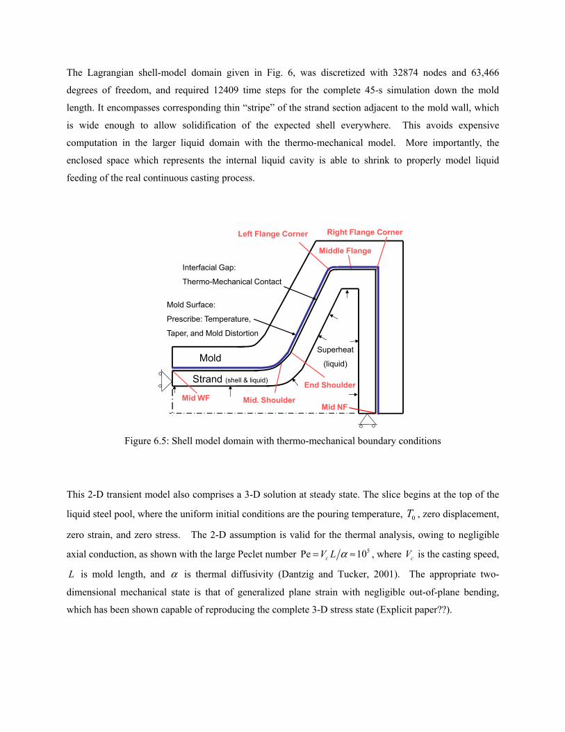
The Lagrangian shell-model domain given in Fig. 6, was discretized with 32874 nodes and 63,466

degrees of freedom, and required 12409 time steps for the complete 45-s simulation down the mold

length. It encompasses corresponding thin “stripe” of the strand section adjacent to the mold wall, which

is wide enough to allow solidification of the expected shell everywhere. This avoids expensive

computation in the larger liquid domain with the thermo-mechanical model. More importantly, the

enclosed space which represents the internal liquid cavity is able to shrink to properly model liquid

feeding of the real continuous casting process.

Figure 6.5: Shell model domain with thermo-mechanical boundary conditions

This 2-D transient model also comprises a 3-D solution at steady state. The slice begins at the top of the

liquid steel pool, where the uniform initial conditions are the pouring temperature, 0T , zero displacement,

zero strain, and zero stress. The 2-D assumption is valid for the thermal analysis, owing to negligible

axial conduction, as shown with the large Peclet number 5Pe 10cV L α= ≈ , where cV is the casting speed,

L is mold length, and α is thermal diffusivity (Dantzig and Tucker, 2001). The appropriate two-

dimensional mechanical state is that of generalized plane strain with negligible out-of-plane bending,

which has been shown capable of reproducing the complete 3-D stress state (Explicit paper??).

Mold Surface:

Prescribe: Temperature,

Taper, and Mold Distortion

Strand (shell & liquid)

Mold

Mid WF Mid. Shoulder

Left Flange Corner Right Flange Corner

Middle Flange

Mid NF

End Shoulder

Superheat

(liquid)

Interfacial Gap:

Thermo-Mechanical Contact

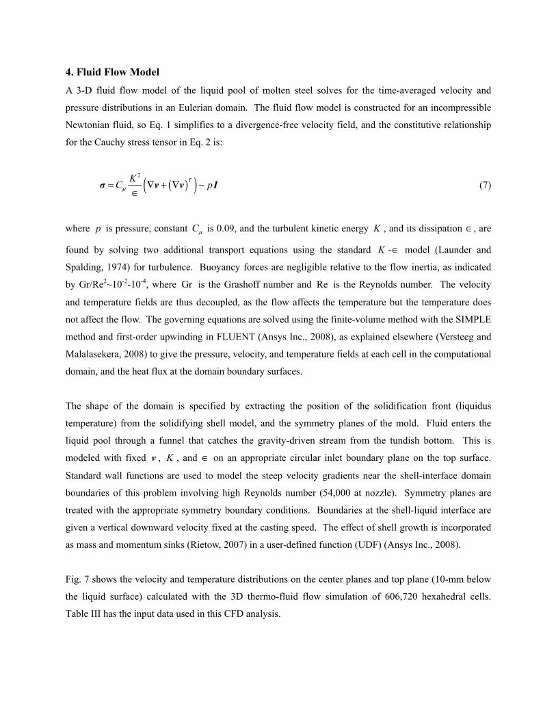
4. Fluid Flow Model

A 3-D fluid flow model of the liquid pool of molten steel solves for the time-averaged velocity and

pressure distributions in an Eulerian domain. The fluid flow model is constructed for an incompressible

Newtonian fluid, so Eq. 1 simplifies to a divergence-free velocity field, and the constitutive relationship

for the Cauchy stress tensor in Eq. 2 is:

( )( )2

TKC pμ= ∇ + ∇ −

∈σ v v I (7)

where p is pressure, constant μC is 0.09, and the turbulent kinetic energy K , and its dissipation ∈, are

found by solving two additional transport equations using the standard K -∈ model (Launder and

Spalding, 1974) for turbulence. Buoyancy forces are negligible relative to the flow inertia, as indicated

by Gr/Re2~10-2-10-4, where Gr is the Grashoff number and Re is the Reynolds number. The velocity

and temperature fields are thus decoupled, as the flow affects the temperature but the temperature does

not affect the flow. The governing equations are solved using the finite-volume method with the SIMPLE

method and first-order upwinding in FLUENT (Ansys Inc., 2008), as explained elsewhere (Versteeg and

Malalasekera, 2008) to give the pressure, velocity, and temperature fields at each cell in the computational

domain, and the heat flux at the domain boundary surfaces.

The shape of the domain is specified by extracting the position of the solidification front (liquidus

temperature) from the solidifying shell model, and the symmetry planes of the mold. Fluid enters the

liquid pool through a funnel that catches the gravity-driven stream from the tundish bottom. This is

modeled with fixed v , K , and ∈ on an appropriate circular inlet boundary plane on the top surface.

Standard wall functions are used to model the steep velocity gradients near the shell-interface domain

boundaries of this problem involving high Reynolds number (54,000 at nozzle). Symmetry planes are

treated with the appropriate symmetry boundary conditions. Boundaries at the shell-liquid interface are

given a vertical downward velocity fixed at the casting speed. The effect of shell growth is incorporated

as mass and momentum sinks (Rietow, 2007) in a user-defined function (UDF) (Ansys Inc., 2008).

Fig. 7 shows the velocity and temperature distributions on the center planes and top plane (10-mm below

the liquid surface) calculated with the 3D thermo-fluid flow simulation of 606,720 hexahedral cells.

Table III has the input data used in this CFD analysis.

Figure 7: Velocity and Temperature Distributions in the Liquid Pool

5. Mold Model

In addition to supporting the shell to determine its shape, the copper mold in the continuous casting

process extracts heat from the molten steel by means of cooling water flowing through circular channels

and rectangular slots. The mold assembly consists of two wide faces, two narrow faces, and their

respective water boxes. The steel water boxes serve to circulate the water in the mold and also increase

the rigidity of the assembly to reduce the effect of the thermal distortion of the mold when it heats up to

operating temperatures. In this work, a three-dimensional finite-element model of one symmetric fourth

of the mold assembly was constructed to capture the effects of mold distortion and variable mold surface

temperature on the solidifying steel shell. The model mold and water box geometries include the

curvature and applied taper of the hot faces, water channels, and bolt holes. The taper is applied to the

mold pieces to accommodate the solidification shrinkage of the solid steel.

X (m)0 0.1 0.2 0.3

Y(m)0

0.10.2

Z(m

)

0

0.1

0.2

0.3

0.4

0.5

0.6

0.5 m/s

0

12963

15

27242118

SuperheatTemperature (C)

The mesh consisted of 263,879 nodes and 1,077,166 tetrahedron, wedge, and hexahedron elements. The

steady-state conservations of energy and momentum in Eqs. 2 and 3 were solved in this model using

ABAQUS (Dassault Corp., 2009). The same constitutive relationship as the shell model was used for the

mold, but the inelastic strain is neglected, owing to the minor role of creep in the copper towards mold

distortion [ref.? G. Li copper paper Met Trans A 2001?]. Contact between the two mold pieces and two

backing plates was enforced manually by iteratively applying constraint equations on contacting nodes.

The mold bolts and tie rods were simulated using linear truss elements and were appropriately pre-

stressed. The heat flux applied to the hot faces of the mold was extracted from the shell-mold surface in

the shell model.

The calculated temperature and distortion results are presented in Figure 6. In addition to providing

insight into thermo-mechanical behavior of the mold, this model provides temperature and displacement

boundary conditions to the shell model. More detail of this model can be found elsewhere (Hibbeler et al.,

2009).

Figure 6. Temperature and distorted shape of mold (20x magnified distortion)

6. Fluid / Shell Interface Treatment

Results from the fluid flow model of the liquid domain affect the solidifying shell model by the heat flux

crossing the boundary, which represents the solidification front, or liquidus temperature. This “superheat

flux” superq can be incorporated into a fixed-grid simulation of heat transfer phenomena in the mushy and

solid regions by enhancing the latent heat (Koric et al., 2010) in Eq. 1. This enables accurate uncoupling

of complex heat-transfer phenomena into separate simulations of the fluid flow region and the mushy-

solid region. Starting with the Stefan interface condition (Dantzig and Tucker, 2001), the additional

latent heat Δ fH to account for superheat flux delivered from the liquid pool can be calculated from:

superf

solid interface

qH

vρΔ = (8)

The latent heat enhancement is added to the original latent heat and enthalpy in Eq. 3 via a UMATHT user

subroutine in ABAQUS (Dassault Corp., 2009). In the transient shell model, the interface speed interfacev

can be estimated from the local cooling rate and temperature gradient at every time and material point

near the solidification front.

1interface

T Tv

T t T

Δ= =∇ Δ ∇

(9)

This method sometimes produces excessive and fluctuating latent heat values when temperature

increments TΔ are driven to be very small by the global NR iterative solution procedures, particularly at

early simulation times and when superheat flux is high. When the maximum latent heat enhancement

reaches 30 to 40 times the initial value of the latent heat, the interfacev estimate switches to an analytical

solution (Koric et al., 2010) based on the classical 1-D solid-control solidification solution (Dantzig and

Tucker, 2001) with the addition of superheat:

( ) ( ) sup2exp erf( )1

φ φ φ πρ α φ

− = +

erp s liq surf f

s

qc T T H

t

(11)

The above equation is solved for φ for every time increment and velocity is calculated as:

( ) φ α=interface sv t t (12)

This method gives an accurate and smooth estimate of the interface velocity, and was shown to perform

well in both one- and two-dimensional solidification problems (Koric et al., 2010).

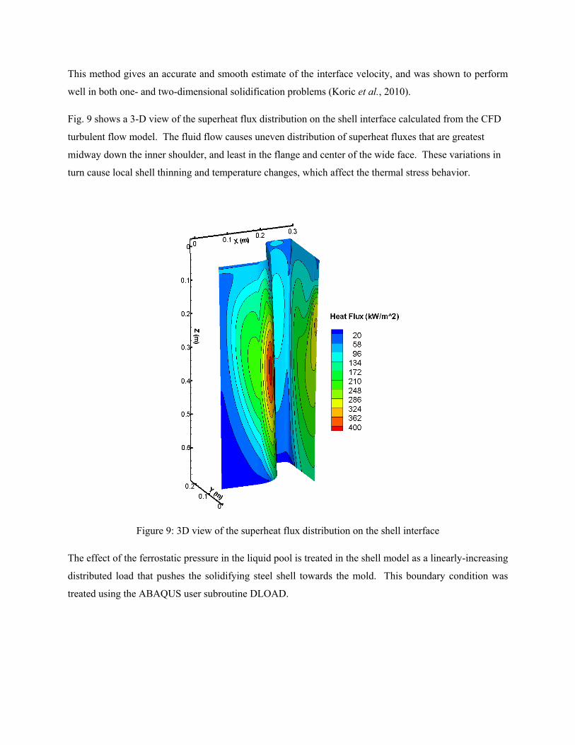
Fig. 9 shows a 3-D view of the superheat flux distribution on the shell interface calculated from the CFD

turbulent flow model. The fluid flow causes uneven distribution of superheat fluxes that are greatest

midway down the inner shoulder, and least in the flange and center of the wide face. These variations in

turn cause local shell thinning and temperature changes, which affect the thermal stress behavior.

Figure 9: 3D view of the superheat flux distribution on the shell interface

The effect of the ferrostatic pressure in the liquid pool is treated in the shell model as a linearly-increasing

distributed load that pushes the solidifying steel shell towards the mold. This boundary condition was

treated using the ABAQUS user subroutine DLOAD.

7. Shell / Mold Interface Treatment

Two-way thermo-mechanical coupling between the shell and mold is needed because the stress analysis

depends on temperature via thermal strains and material properties, and the heat conducted between the

mold and steel strand depends strongly on distance between the separated surfaces calculated from the

mechanical solution. Heat transfer across the interfacial gap between the shell and the mold wall surfaces

is defined with a resistor model that depends on the thickness of gap calculated by the stress model. The

total heat transfer gapq occurs along two parallel paths, due to radiation, radh , and conduction, condh , as

follows:

( )( )/gap rad cond shell moldq k T n h h T T= − ∂ ∂ = − + − (13)

where n is in the direction normal to the surface. The radiation heat transfer coefficient is calculated

across the transparent liquid portion of the mold slag layer:

( )( )2 2

1 11

σ

ε ε

= + ++ −

SBrad shell mold shell mold

shell mold

h T T T T (14)

where 8 2 45.6704 10 Wm Kσ − − −= ⋅SB is the Stefan-Boltzmann constant, 0.8ε ε= =shell mold are the

emissivities of the shell and mold surface, and shellT and moldT are their current temperatures, respectively.

The conduction heat transfer coefficient depends on four resistances connected in series:

( )1 1 1gap slag slag

cond mold air slag shell

d d d

h h k k h

−= + + + (15)

The first resistance, 1 moldh , is the contact resistance between mold wall surface and the solidified mold

slag film. The contact heat transfer coefficient moldh is chosen to be 2500 W/m2 (Park et al., 2002). The

second resistance is associated with conduction across the air gap assuming airk = 0.06 W/m·K. The

thickness of the air gap is determined from the results of the mechanical contact analysis. An artificial

constant slag film thickness, slagd = 0.1 mm, is adopted in this work to prevent non-physical behavior

associated with very small gaps (Park et al., 2002). The third resistance is due to conduction through the

slag film assuming slagk = 1 W/m·K. The final term is the contact resistance between the slag film and

the strand, where the shell contact heat transfer coefficient shellh depends greatly on temperature. This

shell-slag contact coefficient decreases greatly as the shell surface temperature drops below the

solidification temperature of the mold slag (Han et al., 1999). These equations were implemented into

ABAQUS using the user-defined subroutine GAPCON (Dassault Corp., 2009).

The size of the gap is determined through the “softened” exponential contact algorithm built into

ABAQUS/Standard (Dassault Corp., 2009), knowing the position of the mold wall and shell surfaces

xmold and xshell :

( ) ( ) ( ) ( ) ( ), ,gap shell mold shell mold cd t t t t z V= − = −x x p x x p (16)

The first iteration of the shell model used the nominal shape of the mold. For the second iteration of the

shell model, the mold model was post-processed to create a database of surface position, moldx , for points

on the transverse perimeter of the hot face p and time below the meniscus = ct z V . A time-varying

displacement was applied to each point on the hot face to re-create the distorted shape of the mold that the

Lagrangian shell domain would encounter as it moves through the mold, using the ABAQUS user

subroutine DISP.

8. Validation of the Numerical Models

The thermo-mechanical solidification model used in this work was validated by comparison with the

semi-analytical solution of thermal stresses in an unconstrained solidifying plate (Weiner and Boley,

1963). A one-dimensional model of this test casting can produce the complete 3-D stress and strain state

if the condition of generalized plane strain is imposed in both the width (y) and length (z) directions (Li

and Thomas, 2004).

The domain adopted for this problem moves with the strand in a Lagrangian frame of reference as shown

in Fig. 1. The domain consists of a thin slice through the plate thickness using 2-D 4-node generalized

plane strain elements (in the axial z direction) implemented in ABAQUS. The second generalized plane

strain condition was imposed in the y-direction (parallel to the surface) by coupling the displacements of

all nodes along the bottom edge of the slice domain. A fixed temperature is imposed at the left boundary,

with other boundaries insulated.

Figure 1: Solidifying Slice

The material in this problem has elastic-perfectly plastic constitutive behavior. The yield stress drops

linearly with temperature from 20 MPa at 1000 ºC to zero at the solidus temperature 1494.4 ºC, which

was approximated by Yσ =0.03 Mpa at the solidus temperature. A very narrow mushy region, 0.1 ºC, is

used to approximate the single melting temperature assumed in the analytical solution.

Figures 2 and 3 show the temperature and the stress distribution across the solidifying shell at two

different solidification times. More details about this model validation can be found elsewhere (Koric and

Thomas, 2006) including comparisons with other less-efficient integration methods and a convergence

study.

Figure 2: Temperature distribution along the solidifying slice

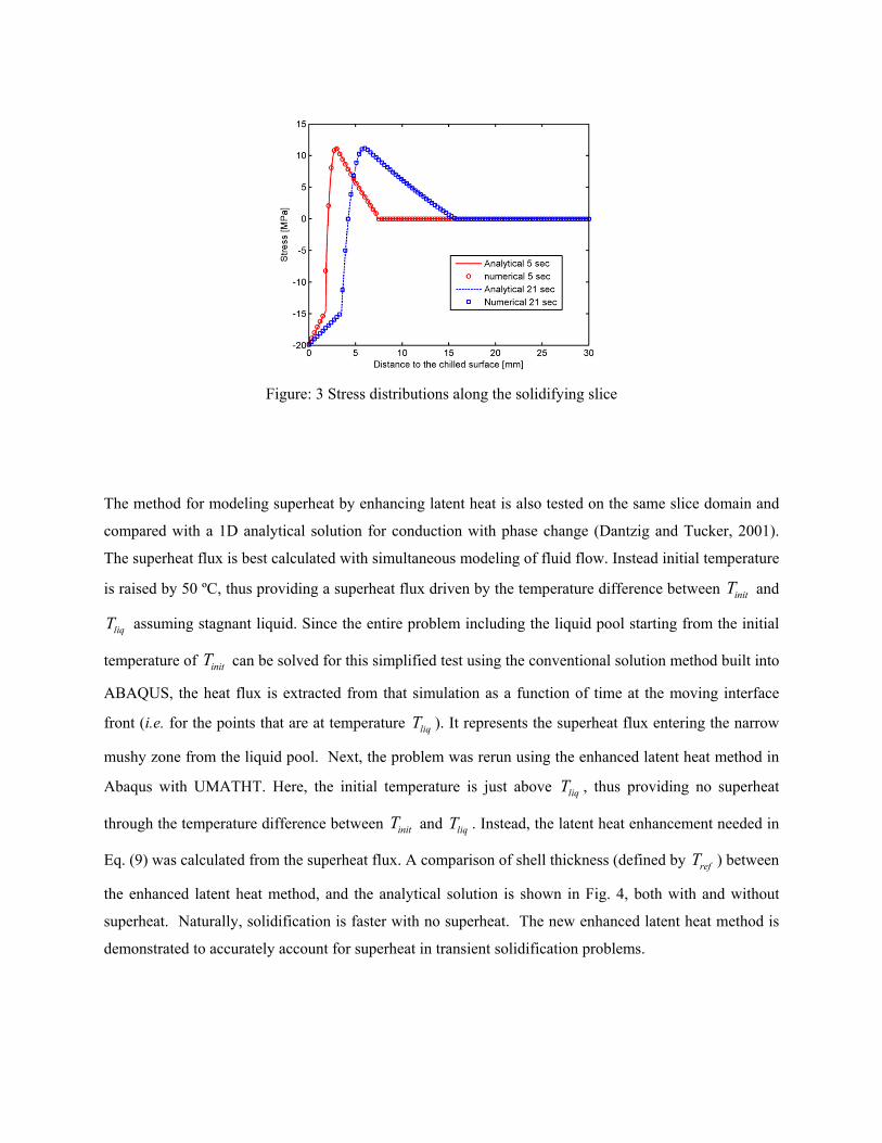
Figure: 3 Stress distributions along the solidifying slice

The method for modeling superheat by enhancing latent heat is also tested on the same slice domain and

compared with a 1D analytical solution for conduction with phase change (Dantzig and Tucker, 2001).

The superheat flux is best calculated with simultaneous modeling of fluid flow. Instead initial temperature

is raised by 50 ºC, thus providing a superheat flux driven by the temperature difference between initT and

liqT assuming stagnant liquid. Since the entire problem including the liquid pool starting from the initial

temperature of initT can be solved for this simplified test using the conventional solution method built into

ABAQUS, the heat flux is extracted from that simulation as a function of time at the moving interface

front (i.e. for the points that are at temperature liqT ). It represents the superheat flux entering the narrow

mushy zone from the liquid pool. Next, the problem was rerun using the enhanced latent heat method in

Abaqus with UMATHT. Here, the initial temperature is just above liqT , thus providing no superheat

through the temperature difference between initT and liqT . Instead, the latent heat enhancement needed in

Eq. (9) was calculated from the superheat flux. A comparison of shell thickness (defined by refT ) between

the enhanced latent heat method, and the analytical solution is shown in Fig. 4, both with and without

superheat. Naturally, solidification is faster with no superheat. The new enhanced latent heat method is

demonstrated to accurately account for superheat in transient solidification problems.

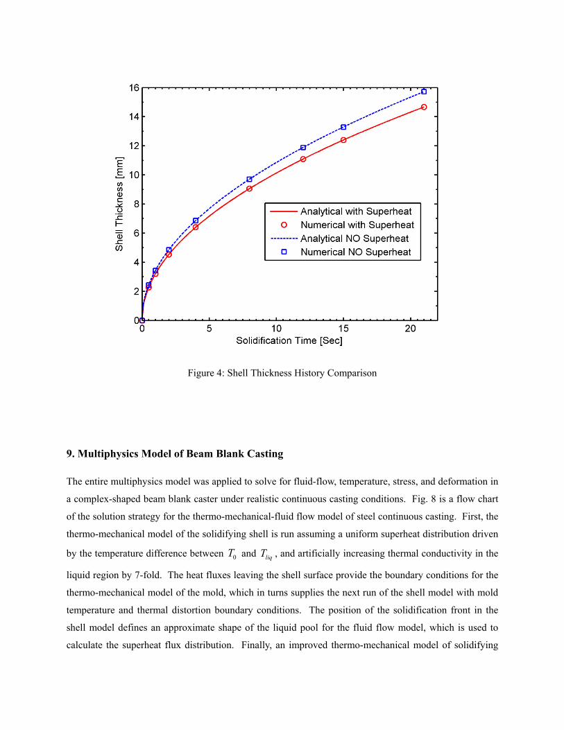
Figure 4: Shell Thickness History Comparison

9. Multiphysics Model of Beam Blank Casting

The entire multiphysics model was applied to solve for fluid-flow, temperature, stress, and deformation in

a complex-shaped beam blank caster under realistic continuous casting conditions. Fig. 8 is a flow chart

of the solution strategy for the thermo-mechanical-fluid flow model of steel continuous casting. First, the

thermo-mechanical model of the solidifying shell is run assuming a uniform superheat distribution driven

by the temperature difference between 0T and liqT , and artificially increasing thermal conductivity in the

liquid region by 7-fold. The heat fluxes leaving the shell surface provide the boundary conditions for the

thermo-mechanical model of the mold, which in turns supplies the next run of the shell model with mold

temperature and thermal distortion boundary conditions. The position of the solidification front in the

shell model defines an approximate shape of the liquid pool for the fluid flow model, which is used to

calculate the superheat flux distribution. Finally, an improved thermo-mechanical model of solidifying

shell is re-run which includes the effects of the superheat distribution and mold distortion, and completes

the first iteration of the multiphysics model. Because the shell profile from the improved thermo-

mechanical model has little effect on superheat results in the liquid pool, a single multiphysics iteration is

sufficient to produce an accurate shell growth prediction.

Figure 8: Flow Chart for Multiphysics Solution Strategy

The shoulder region of the beam-blank mold has a convex shape which converges heat flow and increases

local temperature, opposite to behavior at the corners. Furthermore, a gap in the middle shoulder is caused

by outward bending of the shell due to contact pressure from the mold onto the middle of the flange.

Heat extraction from the shoulder is therefore retarded as shown in Fig. 10, yielding a thinner shell with

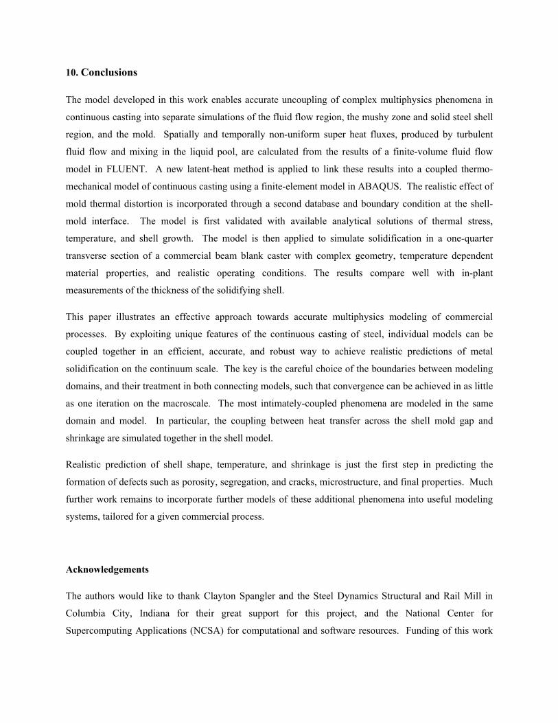
higher temperature. The maximum and minimum principal stress contours at 457 mm (Hibbeler et al.,

2009) are given in Fig. 11. They reveal expected compressive shell behavior at the “cold” surface and

tensile stress in the hot interior near the solidification front, similar to the model validation from Fig. 3.

Maximum stress and strain is found in the shoulder area which is not a surprise since the thinner shell in

Thermo-Mechanical Model ofSolidifying Shell

GAPCON(interfacial BC)

DISP(mold temperature, taper, and distortion )

UMAT(constitutive models

integration)

DLOAD(Ferrostatic Pressure)

Shell Thickness Data to Provide Liquid Pool Shape

UDF(Mass and

Momentum Sink)

CFD Turbulent Model of Liquid Pool

Superheat Flux Data at Liquid/Shell Interface

UMATHT(Converts Superheat into Enhanced Latent Heat)

Heat Flux Data at Mold/Shell Interface

Thermo-Mechanical Model ofMold

Temperature and Distortion Data at Mold Surface

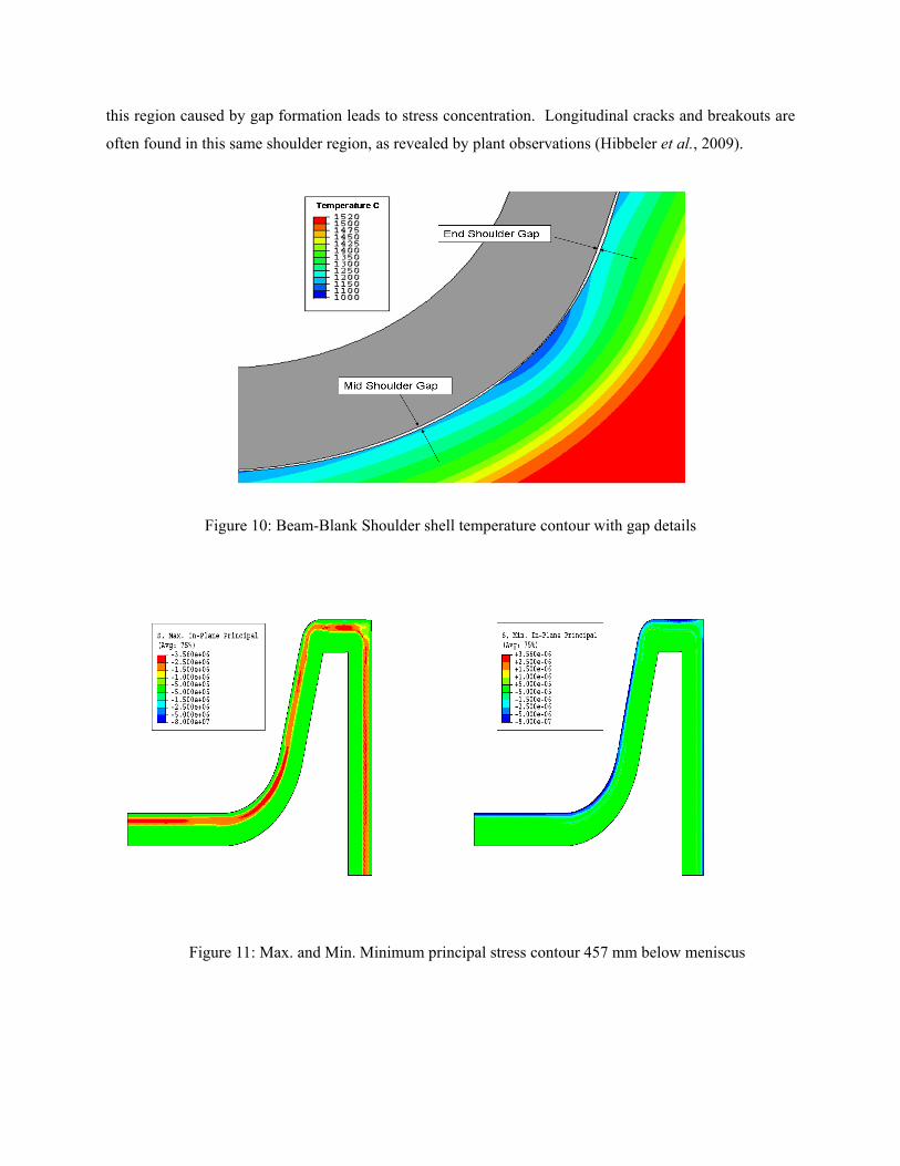
this region caused by gap formation leads to stress concentration. Longitudinal cracks and breakouts are

often found in this same shoulder region, as revealed by plant observations (Hibbeler et al., 2009).

Figure 10: Beam-Blank Shoulder shell temperature contour with gap details

Figure 11: Max. and Min. Minimum principal stress contour 457 mm below meniscus

Finally, the shell thickness at 90% liquid predicted by both models is compared with measurements

around the perimeter of a breakout shell obtained from a commercial caster (Hibbeler et al., 2009) in

Figure 12. The initial thermo-mechanical model assuming a uniform superheat distribution can only

roughly match the shell thickness variations. Shell thickness variations at the corners and shoulder due to

air gap formations were captured owing to the interfacial heat transfer model. However, the middle

portion of the wide face is 4 mm thicker in the measurement. This is evidently caused by the uneven

superheat distribution due to the flow pattern in the liquid pool, as this location is farthest away from the

pouring funnels and has the least amount of superheat as shown in Fig 9. In contrast, the shoulder region

receives the highest amount of superheat, so the measured shell thickness there is more than 2 mm thinner

than the initial thermo-mechanical model prediction. The improved multi-physics model that includes the

fluid flow effects matches the shell thickness measurement around the entire perimeter much more

accurately. This finding illustrates the improved accuracy that is possible by including the effects of fluid

flow into a thermal stress analysis of solidifying shell.

Figure 10: Shell Thickness Comparisons

10. Conclusions

The model developed in this work enables accurate uncoupling of complex multiphysics phenomena in

continuous casting into separate simulations of the fluid flow region, the mushy zone and solid steel shell

region, and the mold. Spatially and temporally non-uniform super heat fluxes, produced by turbulent

fluid flow and mixing in the liquid pool, are calculated from the results of a finite-volume fluid flow

model in FLUENT. A new latent-heat method is applied to link these results into a coupled thermo-

mechanical model of continuous casting using a finite-element model in ABAQUS. The realistic effect of

mold thermal distortion is incorporated through a second database and boundary condition at the shell-

mold interface. The model is first validated with available analytical solutions of thermal stress,

temperature, and shell growth. The model is then applied to simulate solidification in a one-quarter

transverse section of a commercial beam blank caster with complex geometry, temperature dependent

material properties, and realistic operating conditions. The results compare well with in-plant

measurements of the thickness of the solidifying shell.

This paper illustrates an effective approach towards accurate multiphysics modeling of commercial

processes. By exploiting unique features of the continuous casting of steel, individual models can be

coupled together in an efficient, accurate, and robust way to achieve realistic predictions of metal

solidification on the continuum scale. The key is the careful choice of the boundaries between modeling

domains, and their treatment in both connecting models, such that convergence can be achieved in as little

as one iteration on the macroscale. The most intimately-coupled phenomena are modeled in the same

domain and model. In particular, the coupling between heat transfer across the shell mold gap and

shrinkage are simulated together in the shell model.

Realistic prediction of shell shape, temperature, and shrinkage is just the first step in predicting the

formation of defects such as porosity, segregation, and cracks, microstructure, and final properties. Much

further work remains to incorporate further models of these additional phenomena into useful modeling

systems, tailored for a given commercial process.

Acknowledgements

The authors would like to thank Clayton Spangler and the Steel Dynamics Structural and Rail Mill in

Columbia City, Indiana for their great support for this project, and the National Center for

Supercomputing Applications (NCSA) for computational and software resources. Funding of this work

by the Continuous Casting Consortium at the University of Illinois and the National Science Foundation

Grant # CMMI 07-27620 is gratefully acknowledged.

References

Weiner, J. H., Boley, B. A., 1963. Elasto-plastic thermal stresses in a solidifying body. J. Mech. Phys.

Solids. 11,145-154.

Koric, S., Thomas, B. G., Voller, V. R., 2010. Enhanced Latent Heat Method to Incorporate Superheat

Effects into Fixed-grid Multiphysics Simulations. Numerical Heat Transfer Part B, In Press

Koric, S., Thomas, B. G., 2006. Efficient Thermo-Mechanical Model for Solidification Processes.

International Journal for Num. Methods in Eng., 66, 1955-1989.

Dantzig, J. A., Tucker III, C. L, 2001. Modeling in Materials Processing, First ed. Cambridge University

Press, Cambridge, UK.

Zhu, H., 1993. Coupled thermal-mechanical finite-element model with application to initial solidification.

Ph.D Thesis University of Illinois.

Li, C., Thomas B.G., 2004. Thermo-Mechanical Finite-Element Model of Shell Behavior in Continuous

Casting of Steel. Metal. & Material Trans. B., 35B(6), 1151-172.

Grill, A., Brimacombe, J. K, Weinberg, F., 1976. Mathematical analysis of stress in continuous casting of

steel. Ironmaking Steelmaking, 3, 38-47.

Rammerstrofer, F. G.,Jaquemar, C., Fischer, D. F, Wiesinger, H., 1979. Temperature fields, solidification

progress and stress development in the strand during a continuous casting process of steel. Numerical

Methods in Thermal Problems, Pineridge Press, 712-722.

Kristiansson, J. O., 1984. Thermomechanical behavior of the solidifying shell within continuous casting

billet molds- a numerical approach. Journal of Thermal Stresses, 7, 209-226.

Boehmer, J. R., Funk, G., Jordan, M., Fett, F. N., 1998. Strategies for coupled analysis of thermal strain

history during continuous solidification processes. Advances in Engineering Software, 29 (7-9), 679-

97.

Risso, J.M., Huespe, A. E., Cardona, A., 2005. Thermal stress evaluation in the steel continuous casting

process. International Journal of Numerical Methods in Engineering, 65(9), 1355-1377.

Koric, S., Hibbeler, C., L.,Thomas, B., G., 2009. Explicit coupled thermo-mechanical finite element

model of steel solidification, International Journal of Numerical Methods in Engineering ,78, 1-31.

Hibbeler, C., L., Koric, S., Xu, K.,Spangler, C.,Thomas, B., G., 2009. Thermomechanical Modeling of

Beam Blank Casting. Iron and Steel Technology,6(7),60-73.

Lee, J., Yeo, T.,,Kyu, OH, K., H., J. Yoon, J., Yoon, U., 2000. Prediction of Cracks in Continuously Cast

Steel Beam Blank through Fully Coupled Analysis of Fluid Flow, Heat Transfer, and Deformation

Behavior of a Solidifying Shell. Metal. and Materials Transactions A, 31A, 225-237.

Teskeredzic, A.,Demirdzic, I.,Muzaferija, S., 2002. Numerical method for heat transfer, fluid flow, and

stress analysis in phase-change problems. Numerical Heat Transfer B, 42(5), 437-459.

Shamsi, M. R., Ajmani, S. K, 2008. Three Dimensional Turbulent Fluid Flow and Heat Transfer

Mathematical Model for the Analysis of a Continuous Slab Caster. ISIJ International, 47(3), 433-442.

Pokorny, M., Monroe, C., Beckermann, C., Bichler, L., Ravindran, C., 2008. Prediction of Hot Tear

Formation in Magnesium Alloy Permanent Mold Casting,. Int. J. Metalcasting, 2(4), 41-53.

Ho, K., Pehlke, R., D., 1985. Metal-Mold interfacial heat transfer. Metallurgical Transactions B, 16(3),

585-594.

ABAQUS User Manuals v. 6.9, 2009. Dassault Systems Simulia Corp., Providence, RI.

Kozlowski, P., F., Thomas, B., G., Azzi, J. A., Wang, H. 1992. Simple constitutive equations for steel at

high temperature. Metallurgical Transactions, 23A, 903-918.

Voller, V., R., Prakash, C., 1987. A Fixed-Grid Numerical Modeling Methodology for Convection-

Diffusion Mushy Region Phase-Change Problems. Int. J. Heat Mass Transfer, 30, 1709-1720.

Versteeg, H. K., Malalasekera, W., 2008. An Introduction to Computational Fluid Dynamics, Second Ed.,

Pearson Prentice Hall, New York, NY.

Fluent User Manuals v6.3, 2008. Ansys Inc.,Canonsburg, PA.

Rietow, B., 2007. Fluid Velocity Simulations and Measurements in Thin Slab Casting. MS Thesis,

University of Illinois.

Launder, B. E., Spalding, D., B., 1974. The Numerical Computation of Turbulent Flows. Comput.

Methods Appl. Mech. Eng., 3, 269-289.

Park, J., K., Thomas, B., G., Samarasekera, I., 2002. Analysis of Thermo-Mechanical Behavior in Billet

Casting with Different Mold Corner Radii. Ironmaking and Steelmaking, 29(5), 359-375.

Han, H. N., Lee, J. E., Yeo, T. J., Won, Y. M., Kim, K., Oh, K., H., Yoon, J. K. 1999. A Finite Element

Model for 2-Dimensional Slice of Cast Strand. ISIJ International,39(5),445-455.

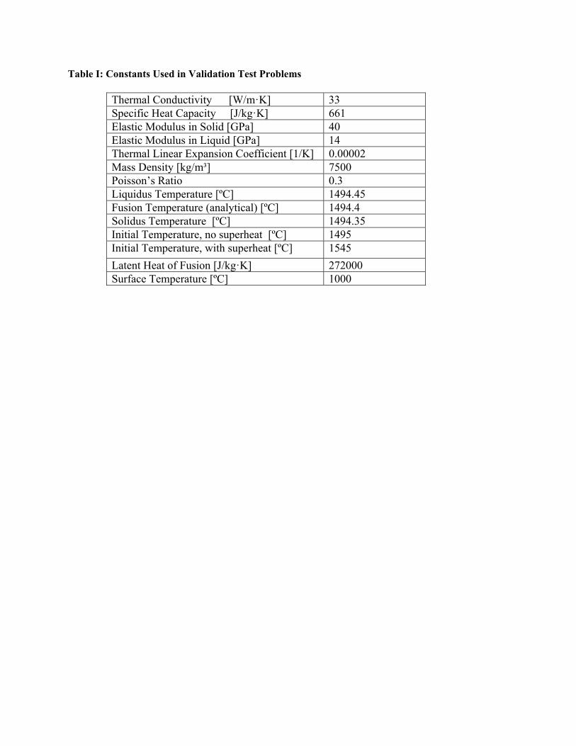
Table I: Constants Used in Validation Test Problems

Thermal Conductivity [W/m·K] 33 Specific Heat Capacity [J/kg·K] 661 Elastic Modulus in Solid [GPa] 40 Elastic Modulus in Liquid [GPa] 14 Thermal Linear Expansion Coefficient [1/K] 0.00002 Mass Density [kg/m³] 7500 Poisson’s Ratio 0.3 Liquidus Temperature [ºC] 1494.45 Fusion Temperature (analytical) [ºC] 1494.4 Solidus Temperature [ºC] 1494.35 Initial Temperature, no superheat [ºC] 1495 Initial Temperature, with superheat [ºC] 1545

Latent Heat of Fusion [J/kg·K] 272000 Surface Temperature [ºC] 1000

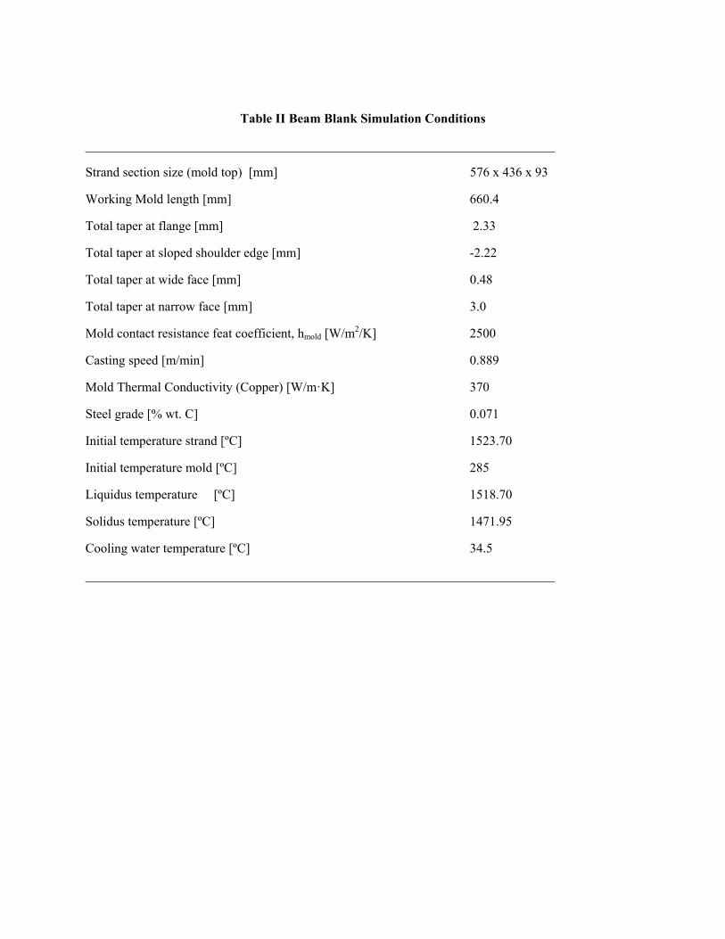
Table II Beam Blank Simulation Conditions

________________________________________________________________________

Strand section size (mold top) [mm] 576 x 436 x 93

Working Mold length [mm] 660.4

Total taper at flange [mm] 2.33

Total taper at sloped shoulder edge [mm] -2.22

Total taper at wide face [mm] 0.48

Total taper at narrow face [mm] 3.0

Mold contact resistance feat coefficient, hmold [W/m2/K] 2500

Casting speed [m/min] 0.889

Mold Thermal Conductivity (Copper) [W/m·K] 370

Steel grade [% wt. C] 0.071

Initial temperature strand [ºC] 1523.70

Initial temperature mold [ºC] 285

Liquidus temperature [ºC] 1518.70

Solidus temperature [ºC] 1471.95

Cooling water temperature [ºC] 34.5

________________________________________________________________________

Table III Fluid Flow Input Data

Density (kg/m3) ρ 6800

Kinetic Viscosity (m2/s) ν 0.006

Inlet Velocity (m/s) vin 1.854

Inlet Diameter (m) d 0.0255

Turbulence intensity at inlet (%) I 200

Inlet kinetic energy (kg*m2/s2) K 0.464

Inlet dissipation rate (m2/s3) ε 2.077

Area of inlet flow (m2) Ain 2.56×10-4

Area of outflow (m2) Al 0.0215

Area of top surface (m2) Am 0.032

Casting Speed (m/s) vC 0.0148