1

Middle East Technical University Mechanical Engineering Department

ME 485 CFD with Finite Volume Method Fall 2019 (Dr. Sert)

ANSYS Fluent Tutorial 4 – Flow over the Ahmed Body Vehicle Model1

Problem Definition

Ahmed Body is a ground vehicle model, frequently used as a benchmark case in experimental and numerical

studies. It was first introduced in a paper by Ahmed et al. in 1984 [1], in which wind tunnel experiments were

performed.

This is a CAD drawing of the Ahmed Body. It

has a curved front, with all other surfaces

being planar. The model is attached to the

ground with four cylinders called stilts. As

seen below, the back part of the top surface

is inclined. Ahmed’s original study [1] has

paid special attention on this inclination

angle called the slant angle by changing it

between 0 and 40 degrees to see its effect on the flow characteristics and the drag force. Reynolds number of

4.29 million was studied in the original paper, corresponding to the free stream air speed of 60 m/s, model

length of 1.044 m and the kinematic viscosity of 1.46×10-5 m2/s.

After the original paper, several researchers performed experimental and numerical studies using this simple

vehicle model. A common modification used in these studies is the reduction of the Reynolds number to 2.86

million, corresponding to the free stream speed of 40 m/s [2]. This is the configuration we are going to simulate

in this tutorial. We will first solve this problem as 2D, using the domain shown in the next page (dimensions are

in meters). The body profile used in this 2D domain is the mid-plane of the 3D model. The slant angle is set to

25o, which is the most commonly studied configuration in the literature. No stilts are used in the 2D model as

they would completely block the flow between the vehicle and the road. Boundary conditions are as follows.

Inlet: 𝑈𝑖𝑛 = 40 m/s, Inlet turbulence intensity = 5 % , Inlet turbulence viscosity ratio = 10

Outlet: 𝑝𝑜𝑢𝑡𝑙𝑒𝑡 = 0

Vehicle surface: No-slip wall

Bottom boundary: No-slip wall

Top boundary: Wall with zero shear (to minimize the wall effects)

Note: Turbulence details given at the inlet are the default values of Fluent, not the ones measured in the

experiments.

1 ANSYS Student 2019 R2 is used to prepare this tutorial.

This document is prepared by Dr. Sert and shared on the website of ME 485 course. You are not allowed to upload it anywhere else.

Reference list is at the end of the tutorial.

If you are an instructor, please ask for permission before using this document in your course.

2

Using the properties of air as used in reference 2 (density is 1.225 kg/m3 and viscosity is 1.787×10-5 m2/s),

Reynolds number based on the model length becomes

𝑅𝑒 =𝜌𝑈𝑖𝑛𝐿

𝜇=

(1.225)(40)(1.044)

1.787 × 10−5= 2.86 million

Reynolds number is sometimes reported in the literature based on the height of the model (0.288 m). In that

case the value becomes 768000.

This tutorial has 2 parts.

• Part 1: 2D Simulation

• Part 2: 3D Simulation

5.044 m

1.044 m 1.4 m

0.288 m

25o 0.1 m

0.1 m

1.0 m

𝑥

𝑦

3.0 m

0.05 m

3

Part 1. 2D Simulation

Step 1a:

Start ANSYS Workbench.

Drag and drop Fluid Flow (Fluent) onto the Project Schematic window.

Change the name of the analysis to Tutorial 4.

Click on the Geometry cell and set its Analysis Type property to 2D.

Right click the Geometry cell, select Import Geometry –> Browse and select the Ahmed Body.scdoc file that you

downloaded from the course web site. The geometry file is already prepared for you.

Step 1b:

Double click the Geometry cell to investigate the imported file in SpaceClaim.

You will see the following drawing. The domain is divided into 4 parts (with the blue lines) to control the mesh

generation process.

Exit SpaceClaim and go back to the Workbench.

Save the project.

4

Step 2a:

Start the Meshing application.

Right click Mesh in the Outline tab and select Insert -> Sizing.

Select the face shown below in purple color and press Apply.

Set the Element Size to 0,005 m. This will control the element size close to the vehicle.

Press the Apply button here.

Select this face

5

Step 2b:

Right click Mesh in the Outline tab and select Insert -> Method.

Select all 4 faces forming the problem domain and press Apply.

Set Method to Triangles.

Press the Apply button here. Select all 4 faces

6

Step 2c:

Create inflation layers over the edges forming the vehicle.

Right click Mesh in the Outline tab and select Insert -> Inflation.

For the Geometry, select the purple face shown below. Press the Apply button.

For the Boundary, select the red edges shown below, i.e. all 7 edges forming the vehicle. Press the Apply button.

Change the Inflation Option to First Layer Thickness.

Set the First Layer Height to 0,0001 m.

Set the Maximum Layers to 20.

Note: To select the 7 edges forming the body, you may first need to press the Edge button in the Toolbar.

Using the Ctrl key, select all these red

edges (7 edges intotal) forming the vehicle

as the Boundary.

Select this face as the Geometry

Press the Apply

buttons here.

7

Step 2d:

Set the number divisions on all the edges forming the vehicle. We need to do this one by one for each face by

right clicking Mesh in the Outline tab and select Insert -> Sizing. Numbers given in the following figure are the

number of divisions for each face.

Note: The body is composed of 7 edges, but in the above screenshot there are 5 edge sizing entries. It is because

two of them are used to set the sizing details of two edges each (the edges with 30 divisions and 200 divisions).

30

30

20

200

200

60

50

These are the number of divisions used

for each edge forming the vehicle.

8

Step 2e:

Put a final edge sizing at the bottom boundary. We’ll specify no-slip condition at the bottom boundary, and it is

possible to put inflation layer there. But we’ll not do that here. Instead we’ll specify the mesh details at the first

part of the bottom boundary as follows.

Select the first edge forming the bottom boundary.

Set Type to Element Size.

Set the Element Size to 0,005 m.

This will allow the boundary layer at the bottom wall to develop more accurately before going under the vehicle.

Select this edge

9

Step 2f:

Generate the mesh.

A mesh of about 100 thousand cells will be generated. Cells outside the inflation layer are triangles.

Following figure shows the inflation mesh details around the curved front part of the body.

10

And this one shows the mesh over the slant surface.

11

Step 2g:

Create the following named selections.

Inlet and outlet are composed of 2 edges each. Use the Ctrl key to select multiple edges.

Bottom is composed of 3 edges. It’s the bottom boundary, i.e. the road.

Top is the upper boundary of the outer rectangular box.

BodyFront is the front part of the vehicle, composed of 3 edges (1 straight and 2 curved edges)

BodyTop is the straight top part of the vehicle.

BodySlant is the 25o inclined part of the vehicle.

BodyBack is the straight back part of the vehicle.

BodyBottom is the straight bottom part of the vehicle.

Save the project.

Exit the Meshing application.

In the Workspace right click the Mesh cell and click Update.

These starting with the word

“body” are the edges of the

vehicle. bodyfront has 3 edges.

12

Step 3a:

Start ANSYS Fluent.

In Fluent’s Launcher window select the Double Precision option.

Also select the Parallel option and set the number of processes to a number that is suitable to your computer.

You can set it to twice the number of cores your computer has. For example, if your computer has a quad core

(4 cores) processor than you can set it as high as 8. In that case all your computer’s computational power will be

used by Fluent. My computer has two cores, and to utilize all the available computational power I set the

Processes value to 4.

Click the OK button.

Note: GPGPU stands for General Purpose Graphics Processing Unit. It is the graphics card of your computer. If

your computer has a powerful graphics card, typically found on gaming machines, Fluent can also utilize that to

perform even faster calculations.

13

Step 3b:

Inside Fluent, under Setup -> General, press the Display button under the mesh options.

Check the Partitions options.

Press the Colors… button and set the color of “surface” type to black.

Press the Display button.

Following partitions will be shown. The mesh is divided into 4 partitions, which is equal to the number of

processes that we selected while launching Fluent. Calculations for each partition will be handled by a separate

computation thread during the parallel solution. The mesh is partitioned such that there are approximately the

same number of cells in each partition to make sure that each process will be kept equally busy during the

calculations.

To Do: Close Fluent and launch it again using different number of processes, such as 2, 3, etc. and display the

partitions created.

14

Step 3c:

We’ll perform a steady, incompressible solution using the pressure based solver. These are already the default

settings.

Under Setup -> Models -> Viscous, set the viscous model to k-omega SST as follows.

15

Step 3d:

The default fluid in Fluent is air. We do not need to change it.

But to be consistent with the reference study, change the viscosity of air to 1.787e-5 kg/(m s) by double clicking

air under Setup -> Materials -> Fluid.

16

Step 3e:

Check the types of the boundary conditions automatically set by Fluent. They should be as follows

• Type of inlet boundary is inlet.

• Type of outlet boundary is pressure-outlet.

• Type of all other boundaries is wall.

At the inlet boundary, set the inlet velocity to 40 m/s.

Leave turbulence details at the inlet as default.

17

Leave the boundary type of the boundary named top as Wall but change its Shear Condition to Specified Shear

and provide zero shear in both directions. This way no boundary layer will develop on the outer top boundary

of the problem domain and this will have minimal effect on the flow field.

Note: If we want to simulate the conditions of a wind tunnel experiment, we could have created the problem

domain in the exact size of the wind tunnel test section and assign slip wall BC at the top boundary. But that is

not the aim here.

At the outlet boundary, keep the default value of zero gauge pressure.

All other boundaries (bottom, bodyfront, bodyback, bodyslant, bodybottom, bodytop) should be of wall type

with no-slip condition specified.

18

Step 3f:

Set the Reference Values as follows. These are important because they will be used to calculate the drag

coefficient. Reference area is the frontal projected area of the vehicle. Assuming unity depth in the 𝑧 direction,

the area is equal to the height of the model, which is 0.288 m.

19

Step 3g:

Under Solution -> Methods, change the last two settings related to the transport equations of turbulence

modeling to second order upwind.

Note: Under the Gradient setting, there are three options. These are the

available gradient reconstruction techniques. They are used to calculate the

gradient ∇𝜙 at the cell centers and cell faces. They are a very important part

of the FVM calculations on unstructured meshes. Least Squares Cell Based is

the default option and we use it in this tutorial.

Note: Under the Momentum setting, there are four options. These are the

available schemes used to calculate the convection term of the linear

momentum conservation equation. Power Law is a hybrid scheme combining

central discretization and some sort of upwinding depending on the cell Peclet

number. MUSCL (Monotone Upstream-Centered Schemes for Conservation

Laws) is another popular scheme and it is a blend of second order upwind and

central schemes. Second Order Upwind is the default option and we use it in

this tutorial. But make sure that it is not exactly the same as the SOU scheme we studied in our lectures. It is

more like a TVD scheme.

You can read about all these schemes in 28.3.1 Spatial Discretization section of Fluent’s Theory Guide.

20

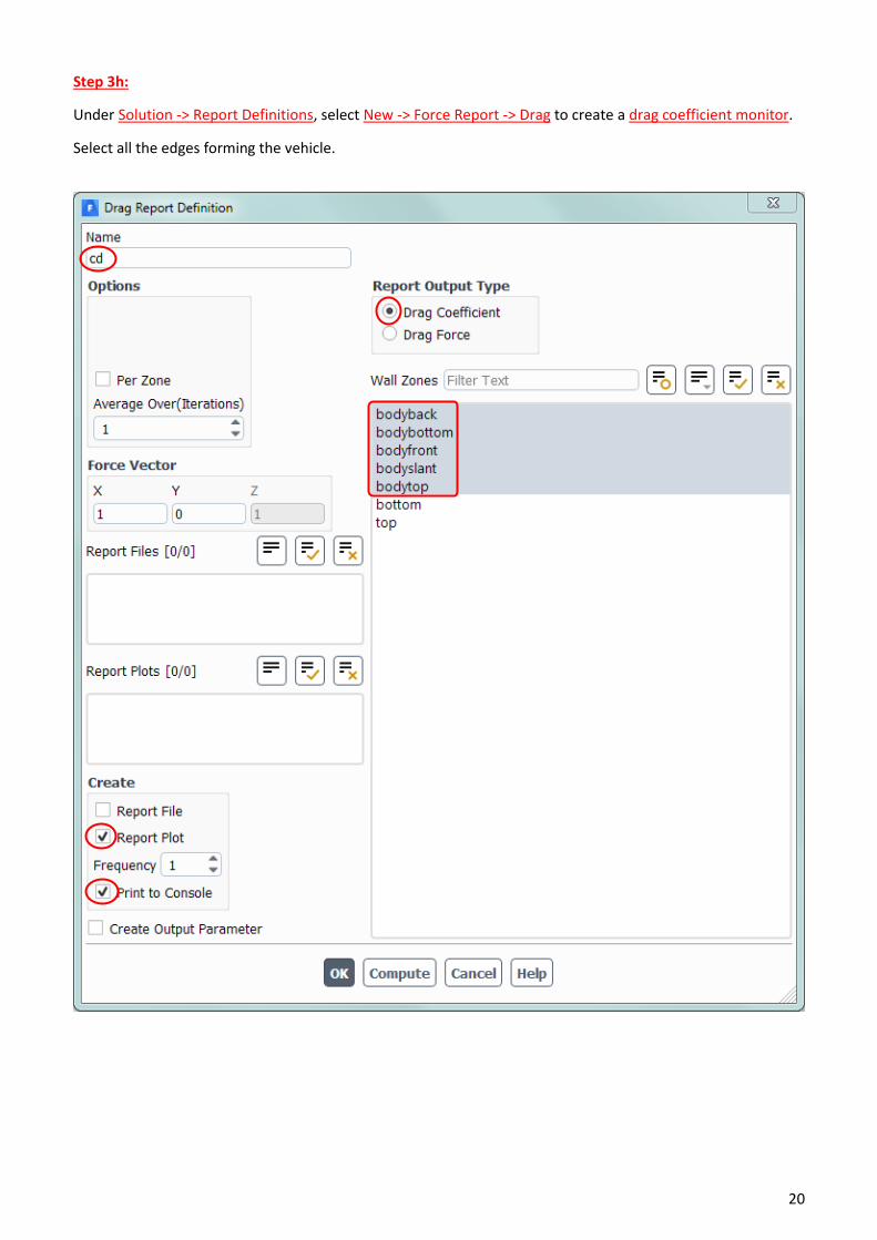
Step 3h:

Under Solution -> Report Definitions, select New -> Force Report -> Drag to create a drag coefficient monitor.

Select all the edges forming the vehicle.

21

Step 3h:

Initialize the solution with Hybrid Initialization.

Set the number of iterations to 1000 and Calculate the solution.

Convergence will be achieved in about 100 iterations.

Cd monitor plot is as follows. It converged to a value around 0.54.

𝐶𝑑 converged to 0.54

22

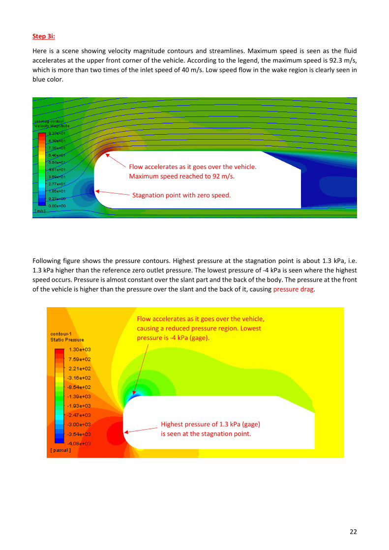
Step 3i:

Here is a scene showing velocity magnitude contours and streamlines. Maximum speed is seen as the fluid

accelerates at the upper front corner of the vehicle. According to the legend, the maximum speed is 92.3 m/s,

which is more than two times of the inlet speed of 40 m/s. Low speed flow in the wake region is clearly seen in

blue color.

Following figure shows the pressure contours. Highest pressure at the stagnation point is about 1.3 kPa, i.e.

1.3 kPa higher than the reference zero outlet pressure. The lowest pressure of -4 kPa is seen where the highest

speed occurs. Pressure is almost constant over the slant part and the back of the body. The pressure at the front

of the vehicle is higher than the pressure over the slant and the back of it, causing pressure drag.

Flow accelerates as it goes over the vehicle,

causing a reduced pressure region. Lowest

pressure is -4 kPa (gage).

Highest pressure of 1.3 kPa (gage)

is seen at the stagnation point.

Flow accelerates as it goes over the vehicle.

Maximum speed reached to 92 m/s.

Stagnation point with zero speed.

23

Step 3j:

Below, we see the boundary layer velocity profiles at the upper front part of the vehicle. These are drawn using

Results -> Graphics -> Vectors, by setting the Style to arrow and Scale to 0.15.

Velocity vectors over the start part is seen in the following zoomed in figure. Flow separates almost at the

beginning of the slant surface and backflow is seen over the whole slant.

Backflow

20 layers of inflation mesh covers this part. The structured

inflation layer mesh is recognized easily by the organized vectors.

Boundar layer thickness is roughly

about this much at this location.

24

Step 3k:

Following figure shows the variation of wall y-plus on the bottom, top and slant parts of the vehicle. It is created

using Results -> Plots -> XY Plots. On the top and bottom walls, y-plus varies between 3 and 8, which means we

are not resolving the viscous sublayer, which is between 0 < 𝑦+ < 5, properly. The values are smaller over the

slant part due to the lower speeds in the backflow, i.e. lower shear stress. Remember that we used a first layer

thickness of 0.1 mm to create the inflation layer mesh. A smaller value is necessary to resolve the viscous

sublayer over the top and bottom walls. But the important question is whether it is necessary or not and how

will the solution, such as the 𝐶𝑑 value, change when we do that?

Note: As discussed in the previous tutorial, Fluent tries to automate the near wall treatment using what it calls

y+ insensitive wall treatment for the k-omega RANS model. It uses no wall functions when the mesh is fine

enough and wall y-plus values are low enough, and it makes use of the universal law of the wall otherwise. Also

note that in section 12.2.1.11. Grid Resolution for RANS Models of Fluent’s User’s Guide it says

“Generally speaking, it is more important to ensure that the boundary layer is covered with sufficient

cells, then to achieve a certain y-plus criterion”.

And in the same section “the sufficient number of layers” is mentioned as at least 10. There are more than 10

layers inside the boundary layers of our mesh.

Top of the vehicle

Slant of the vehicle

Bottom of the vehicle

25

Step 3l:

Under Results -> Reports -> Forces, select all the surfaces forming the vehicle and calculate the forces acting on

them.

The result is as follows

As seen, the pressure drag accounts for 93% of the total drag force. Viscous drag contribution is only 7%.

Pressure drag on the back and slant surfaces are seen as positive values. Gage pressure there is negative and

the gage pressure force does not act into the vehicle, but acts away from the vehicle, causing positive pressure

drag. Similarly, in the above table the pressure drag on the front part of the vehicle is negative. The average

gage pressure on the front of the vehicle is again negative (yes, this is the case), again resulting in pressure drag

force acting away from the front surface. And this causes a negative drag force.

Pressure

drag Viscous

drag

Total

drag

26

To check the results given in the above table, we can use Results -> Reports -> Surface Integrals. For example,

we can calculate the area and the average pressure on the back surface of the vehicle as follows.

Multiplying the calculated area and the pressure we get the following pressure force

𝐹𝑝𝑏𝑎𝑐𝑘= (0.194)(−541.6073) = −105.0718 N

which is exactly the value of the pressure drag force acting on the back part of the vehicle reported in the table

of the previous page. Minus sign means that the force is acting not into the surface but away from the surface,

i.e. in 𝑥 direction, causing positive drag force.

To Do: Calculate the area and the average pressure of the slant surface of the vehicle and combining them with

the 25o slant angle, calculate the pressure drag force acting on it. Compare the value with 60.16 N reported in

the table of the previous page.

27

Step 3m:

In the original Ahmed Body paper [1], variation of the drag coefficient

𝐶𝑑 with the slant angle 𝜃 is given as shown on the right. Starting from

0.25 at zero slant angle, it first decreases making a minimum at around

10o. It then increases up to 0.38 at 30o, which is a critical angle above

which the flow characteristic in the wake of the vehicle changes

considerably, resulting in a sudden drop of 𝐶𝑑. For the 25o angle case

studied in this tutorial, reference [1] reports a 𝐶𝑑 value of about 0.285.

The value we obtained, 0.54, is too high compared to this value.

Following table is taken from the CFD study of Guilmineau et al. [2], where the problem is solved using four

different turbulence models (𝑘 − 𝜔 SST and EARSM are RANS type models and DES and IDDES are hybrid RANS-

LES solutions) and the obtained 𝐶𝑑 values are compared with 3 different experiments (Reference 4 in the

following table is the original paper of Ahmed et al.). As seen, there is considerable deviation between the

results. Even the experimental values differ up to 30%. But still all them are much lower than the one we

calculated.

0.38

0.26 0.25

0.23

0.1

0.3

0.2

0 0 10 20 30 40

𝜃 [°]

𝐶𝑑

0.4

28

Step 3n:

Following figure is Fig. 17 of reference [2] and it shows the streamlines in the wake region behind the vehicle

obtained using different turbulence models. Wake region is important because the dominant drag component

is the pressure drag, which depends a lot to the flow pattern inside the wake region. Note that all the results

shown below are coming from 3D simulations and what we see are the streamlines at the mid-plane of the body.

The top two plots are for the RANS models and they predict larger circulation regions than those predicted by

the hybrid DES techniques and the experiment. As you see, flow field in the wake of the vehicle is predicted

quite different by different models.

Note: In reference [2] both 25o and 35o slant angles are studied. Be careful in using that reference.

This result shows reattachment

on the slant surface. And the

wake region is much smaller.

Our result, shown on the next

page, looks similar to this one.

DES and IDDES results look

the most similar to this

measurement.

29

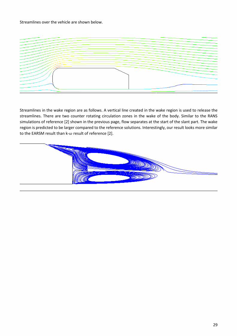
Streamlines over the vehicle are shown below.

Streamlines in the wake region are as follows. A vertical line created in the wake region is used to release the

streamlines. There are two counter rotating circulation zones in the wake of the body. Similar to the RANS

simulations of reference [2] shown in the previous page, flow separates at the start of the slant part. The wake

region is predicted to be larger compared to the reference solutions. Interestingly, our result looks more similar

to the EARSM result than k-𝜔 result of reference [2].

30

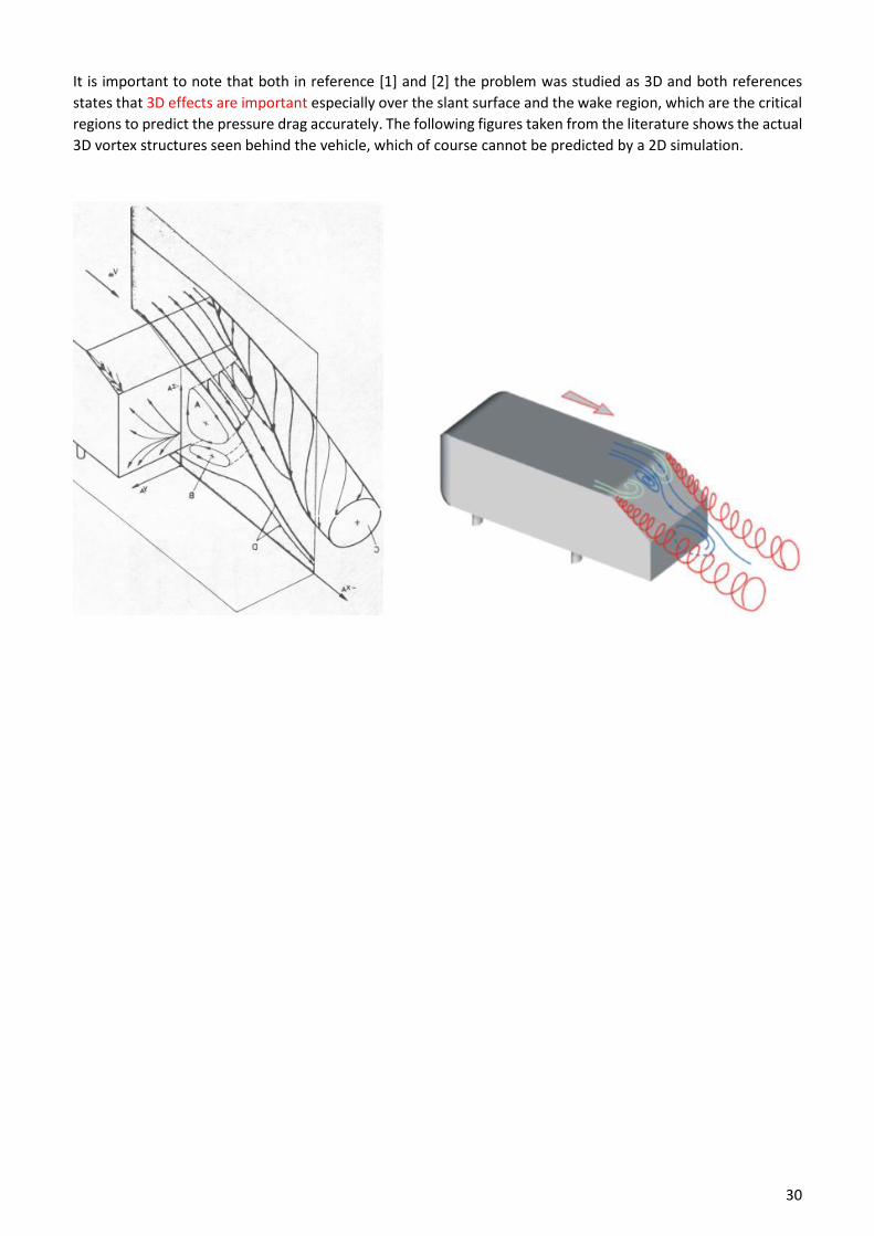
It is important to note that both in reference [1] and [2] the problem was studied as 3D and both references

states that 3D effects are important especially over the slant surface and the wake region, which are the critical

regions to predict the pressure drag accurately. The following figures taken from the literature shows the actual

3D vortex structures seen behind the vehicle, which of course cannot be predicted by a 2D simulation.

31

Part 2. 3D Simulation

The 2D simulation we performed resulted in a drag coefficient that is much larger than those reported in the

literature. Let’s now perform a 3D simulation. Here the main problem is that the student version of ANSYS Fluent

does not allow using meshes with more than 512000 cells. To compare, three different meshes with 7, 12 and

23 million cells were used in the 3D simulations performed in reference [2]. Therefore, we should not expect

much from a 3D simulation with only 512000 cells, but let’s try and see if we can capture the 3D vortical

structures in the wake region or not and if we can get a lower 𝐶𝑑 value.

To limit the number of cells in our mesh as much as possible, we will use only half of the 3D Ahmed Body, as

shown below with symmetry boundary condition on 𝑧 = 0 plane. This is a valid simplification considering that

the flow in both halves are expected to be the same. The blue region of the figure shows the fluid region, i.e.

the vehicle is taken out from the rectangular outer box. Origin is at the bottom rear corner of the vehicle. The

size of the outer box and the positioning of the body in it are similar to those used in the 2D model. But now

there is the depth in the third dimension, which is taken as 0.9 m. The half width of the vehicle in the 𝑧 direction

is 0.1945 m.

Different than the 2D model, this 3D model

has two stilts, i.e. small circular supports that

are used in the original experiment to attach

the body to the bottom wall. Actually, there

are 4 stilts in the original model as seen in

the first page of this tutorial, but our half

model has only 2 of them.

0.1945 m

Circular stilts (supports) join the

bottom surface of the vehicle to the

bottom of the problem domain.

Symmetry

plane

32

Step 4:

Start a new Workbench session and insert a Fluent analysis into it.

Step 5:

Right click the Geometry cell in the Workbench, select Import Geometry –> Browse and select the downloaded

AhmedBody3D.scdoc file.

If you want, you can examine the imported geometry in SpaceClaim.

To control mesh sizing, the problem domain is divided into 7 parts and the one shown below in orange color is

named as Refinement Box.

Note: The problem domain is divided into not 6 but 7 parts. One of the parts is not seen in the above view

because it is at the back of the orange part.

0.1945 m

(half width of

the vehicle)

This orange part is named as the

“Refinement Box”. Finer mesh

will be generated in this region.

33

Step 6a:

Start the Meshing application.

Add the following sizing controls.

Face Sizing: Insert -> Sizing. Select the 11 faces forming the vehicle including the stilts. Set

element size to 0.01 m.

Body Sizing: Insert -> Sizing. Select the Refinement Box (volume). Set element size to 0.025 m.

Body Sizing 2: Insert -> Sizing. Select all the bodies (volumes) other than the Refinement Box

(totally select 6 bodies). Set element size to 0.2 m.

Patch Conforming Method: Insert -> Method. Select all 7 bodies (volumes) forming the problem domain. Set

method to Tetrahedrons.

Generate the mesh. Following mesh of about 480000 cells will be generated.

34

Here is a zoomed in view of the mesh around the vehicle.

Note: No inflation layer is generated due to the element number limitation of the student version of ANSYS.

35

Step 6b:

Create the following named selections.

Inlet: Composed of 2 faces.

Outlet: Composed of 2 faces.

Symmetry: Composed of 6 faces.

Top: Composed of 3 faces.

Side: Compose of 6 faces. This is the side wall (opposite of the symmetry plane) of the problem domain.

Bottom: Composed of 4 faces.

Vehicle: Composed of 11 faces (including the side wall of the vehicle and the circular stilts).

Warning: Be careful in creating these named selections. They have to be correct.

36

Step 7a:

Save the project.

Close the meshing application.

In the Workbench, update the Mesh cell.

Start Fluent (activate double precision and parallelization).

Set viscous model to k-omega SST.

Set air viscosity to 1.787x10-5 m2/s.

Set the inlet speed to 40 m/s. Inlet BC is specified at 2 faces.

Set the boundary type of the top boundary to wall with zero shear. There are 2 faces at the top boundary.

Set the boundary type of the side boundary to wall with zero shear. There are 3 faces at the side boundary.

Important: Fluent assigns certain BCs to all boundary faces by looking at the names we used in “named

selections”. For example, if we name a face as “symmetry” Fluent assigns symmetry BC there. But if we misspell

the name, e.g. call it “symyetry”, then the default BC type of wall may be assigned there. So be careful and check

all BC types.

Inlet

Outlet

Symmetry

Zero shear wall

Zero shear wall

37

Under Setup -> Reference Values, set the reference area to 0.056 m2 and the reference speed to 40 m/s.

Note: The frontal projected area of the half 3D model is 0.288 x 0.1945 = 0.056 m2.

Create a force report for Cd. Select vehicle as the surface.

Initialize and Calculate the solution by setting the Number of Iterations to 1000.

Unfortunately, convergence cannot be achieved. Residual plot after about 500 iterations is as follows. The

continuity residual stalls at about 10−2 and does not fall below the default tolerance of 10−3.

The drag coefficient monitor is given below. Oscillations seen are a sign of convergence problems. 𝐶𝑑 oscillates

around 0.35, which is a value much closer to the experimental value.

Important: What is the reason of the convergence difficulty? There may be unsteadiness due to vortex shedding

at the wake of the vehicle. There can be quality problems in the mesh. Or the mesh may not be fine enough in

required regions.

Continuity equation is not converging

𝐶𝑑 oscillates around 0.33

38

Step 7b:

This is a good chance for us to experiment with discretization schemes and see how they affect convergence.

Save the project and close Fluent.

In the Workbench right click “Fluid Flow (Fluent)” cell and select Duplicate.

Double click the Setup cell of the second analysis to start Fluent.

Duplicate

39

Step 7c:

Under Solution -> Methods, change Momentum discretization scheme to First Order Upwind.

Note: Momentum discretization scheme refers to the way the convective term in the conservation of linear

momentum is discretized. By default, it was Second Order Upwind and we are changing it here. But the

convective terms of the transport equations of Turbulent Kinetic Energy (𝑘) and Specific Dissipation Rate (𝜔)

were already First Order Upwind and we haven’t changed them.

Note: The Second Order Upwind used in Fluent is not exactly the SOU we studied in class. It is more like a TVD

scheme.

40

Step 7d:

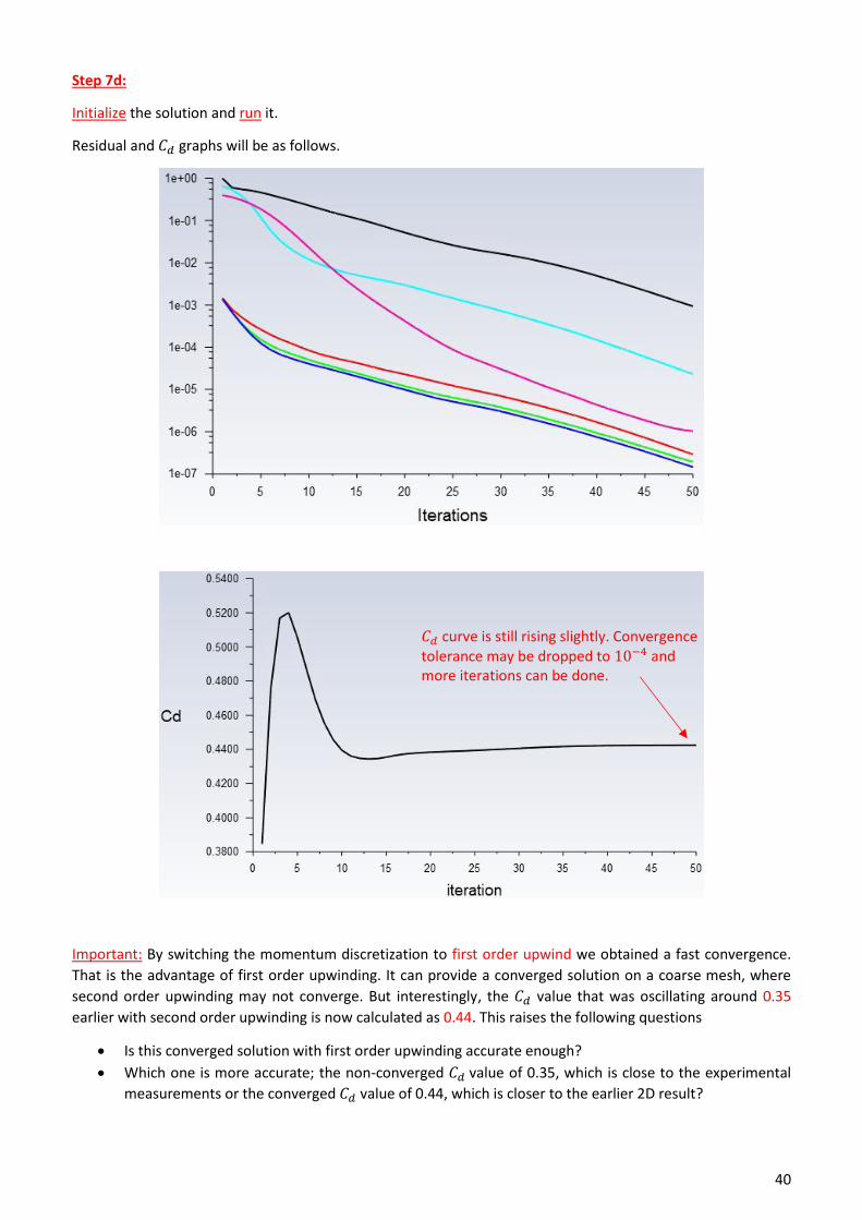
Initialize the solution and run it.

Residual and 𝐶𝑑 graphs will be as follows.

Important: By switching the momentum discretization to first order upwind we obtained a fast convergence.

That is the advantage of first order upwinding. It can provide a converged solution on a coarse mesh, where

second order upwinding may not converge. But interestingly, the 𝐶𝑑 value that was oscillating around 0.35

earlier with second order upwinding is now calculated as 0.44. This raises the following questions

• Is this converged solution with first order upwinding accurate enough?

• Which one is more accurate; the non-converged 𝐶𝑑 value of 0.35, which is close to the experimental

measurements or the converged 𝐶𝑑 value of 0.44, which is closer to the earlier 2D result?

𝐶𝑑 curve is still rising slightly. Convergence tolerance may be dropped to 10−4 and more iterations can be done.

41

Following tables are for the 3D solutions with SOU and FOU discretizations for momentum. They show pressure

and viscous components of drag force and are obtained in Fluent using Results -> Reports -> Forces.

Momentum with SOU:

Momentum with FOU:

Both the pressure and the viscous components of the drag force are higher for FOU. Pressure drag is 1.38 times

higher and viscous drag is 1.11 times higher. Therefore, the main difference in 𝐶𝑑 seemed to be caused by the

pressure drag.

42

Step 8a:

Let’s compare the two 3D solutions side by side in CFD-Post.

Save the project and close Fluent.

In the Workbench rename the second Fluent analysis Tutorial 4 3D FOU.

Find Results in the Toolbox under Component Systems and drop it on the Project Schematics.

Join the Solutions cells of the two Fluent analysis to the new Results cells.

Double click the new Results cell to open CFD-Post.

Form these links.

First rename this.

43

Step 8b:

Both 3D results will be shown side by side.

Click this Synchronize camera in displayed views button for easier comparison.

Select Contour from the Insert menu.

Set Locations to vehicle.

Set Variable to pressure.

Press the Apply button.

As seen, the pressure contours over the vehicle are very similar.

44

Let’s plot the contours of the two solutions separately to see the individual min and max pressure values.

First change the Domains settings of Contour 1 to All Tutorial 4 3D Domains.

Change Range to Local.

Press the Apply button.

The minimum and maximum gage pressures are -2714 Pa and 1016 Pa.

Now change the Domains settings of Contour 1 to All Tutorial 4 3D FOU Domains.

Press the Apply button.

The minimum and maximum gage pressures are -2421 Pa and 1025 Pa.

Although pressure contours seem to be very similar, there are differences in the values and this apparently

creates a 1.38 times difference in pressure drag as reported previously in page 41.

To Do: How these quite similar pressure contours result in this 1.38 times difference needs a more careful

investigation.

45

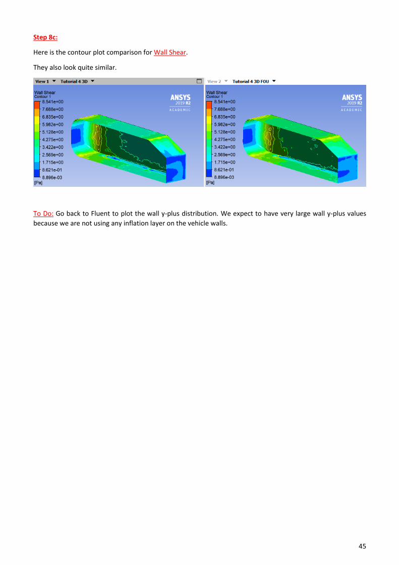
Step 8c:

Here is the contour plot comparison for Wall Shear.

They also look quite similar.

To Do: Go back to Fluent to plot the wall y-plus distribution. We expect to have very large wall y-plus values

because we are not using any inflation layer on the vehicle walls.

46

Step 8d:

To see the streamlines in the wake region, let’s first create a line there.

Select Insert -> Location -> Line from the menu and enter the coordinates as follows. This will create a line at

the symmetry plane.

To draw streamlines, select Insert -> Streamlines from the menu.

Set Surfaces to symmetry component 1 refinement box.

Change Max Points to 250.

Set Locations to the line created above called Line 1 and set Direction to Forward and Backward.

47

Pressing Apply will create the following figure. To see this, make sure that the Streamline 1 entry in the Outline

tab is checked.

Streamline patterns are also very similar.

Zoomed in view of the first plot at the back of the vehicle are as follows

Important: Similar to the 2D solution, there are two counter rotating circulation zones in the wake region. But

they are much smaller than the 2D ones. The flow over the slant part is not separated but attached. These

streamlines are similar to the experimental ones shown at page 28. But interestingly, they are not similar to the

3D k-omega SST result of the reference study given in the same page. Remember that the mesh used here is

much coarser than the one used in the reference.

Unlike the 2D case, flow

over the slant is attached.

Circulation zone is much

smaller than the 2D case.

48

Step 8e:

To visualize the rotating flow structures behind the body use Insert -> Location -> Isosurface.

Set Variable to Velocity.CurlX, (you can select it from the list of all available variables by clicking the “…” button

next to the Variable box).

Set Value to 150 s-1, which is a number selected after a few trials.

Pressing the Apply button will show the following rotating vortical structure originating from the corner of the

slant and filling the wake region of the body. The pattern seen below is similar to the one sketched in page 30.

What we see is the iso-surface where the 𝑥 component of the curl of the velocity vector has a value of 150.

Although the vortical structure can be seen, it is hard to claim that it is captured accurately due to the coarse

mesh we have in the wake of the body.

Note that another rotating structure also originates from the bottom front corner of the vehicle and it elongates

all the way to the wake region to get combined with the one originating from the rear upper corner.

Also note that we are modeling half of the width of the vehicle and no such vortices originate from the corners

of the symmetry plane because they are not really corners.

Vortical structure originating

from the corner of the slant

Another vortical structure

originating from the bottom

front corner of the vehicle

49

Step 8f:

Let’s plot contours of 𝑢 velocity component on the vertical planes at the back of the vehicle and compare them

with those given in reference 2.

First insert a plane using Insert -> Location -> Plane.

Set Method to YZ plane.

Set X to zero.

This will create a vertical plane passing through the back surface of the vehicle. Note that the origin of the 3D

model is at the back bottom of the of the car.

Insert a new contour plot.

Set Locations to Plane 1, the vertical plane we just created.

Set Variable to Velocity u.

Set Range to User Specified and change the Min and Max values to -10 and 40, to be consistent with the figure

given in the reference paper.

Press the Apply button to get the following plot.

Compare this with the following one obtained from reference 2. This one shows the whole vehicle width, not

half of it. As you see, our coarse mesh solution cannot capture the details seen in the reference solution.

Back of

the car

k-𝜔 SST solution

of reference 2

50

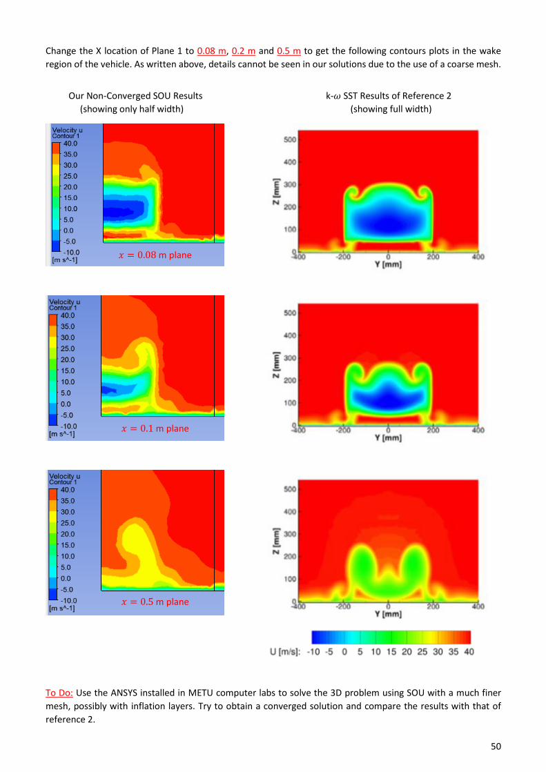
Change the X location of Plane 1 to 0.08 m, 0.2 m and 0.5 m to get the following contours plots in the wake

region of the vehicle. As written above, details cannot be seen in our solutions due to the use of a coarse mesh.

Our Non-Converged SOU Results k-𝜔 SST Results of Reference 2

(showing only half width) (showing full width)

To Do: Use the ANSYS installed in METU computer labs to solve the 3D problem using SOU with a much finer

mesh, possibly with inflation layers. Try to obtain a converged solution and compare the results with that of

reference 2.

𝑥 = 0.08 m plane

𝑥 = 0.1 m plane

𝑥 = 0.5 m plane

51

References:

[1] S. R. Ahmed, G. Ramm, G. Faltin, “Some Salient Features of the Time-Averaged Ground Vehicle Wake”, SAE

Technical Paper 840300, 1984.

[2] E. Guilmineau et al., “Assessment of Hybrid RANS-LES Formulations for Flow Simulation around the Ahmed

Body”, Computers and Fluids, Vol. 176, pp. 302-319, 2018.