Express Introductory Training in ANSYS Fluent be exported from ANSYS Meshing; the "Mesh" cell B2 to...

© 2013 SimTec Ltd. September 23, 2013 1 Release 14.5.7

PRACE Autumn School 2013 – Industry Oriented HPC Simulations, September 21–27,

University of Ljubljana, Faculty of Mechanical Engineering, Ljubljana, Slovenia

Express Introductory Training in ANSYS Fluent

HPC Workshop

HPC with ANSYS Fluent

Dimitrios Sofialidis

Technical Manager, SimTec Ltd.

Mechanical Engineer, PhD


14.5 Release

HPC WorkshopHPC with ANSYS Fluent


Workshop Description:

This workshop deals with external aerodynamic around a generic SUV car travelling at 180 [km/h]. This type of simulations require large meshes and considerable computing power, in order to provide accurate results in a reasonable time.

Learning Aims:

This workshop aims to teach basic procedures in running parallel jobs in ANSYS Fluent. A relatively coarse and a finer mesh will be employed and a comparison will be made on computer performance on both meshes. Various issues will be discussed, connected with computing performance (mesh size, transient vs steady–state run, y+ value at walls connected to the turbulence model used, etc.) and a few tricks to accelerate solution and save CPU time will be mentioned.

Learning Objectives:

To learn how to perform parallel runs in ANSYS Fluent.

Introduction


Start a WB Session and load a Project

• Start ANSYS Workbench (AWB), by issuing command "runwb2" in a Terminal. First,you need to issue command "module load ansys" and then command "node" (tohave a full node at your disposal).

• "File>Restore Archive…" browse to the sub–dir "3.HPC_WORKSHOP" and selectarchived AWB project "car_ext_aero_UNSOLVED.wbpz" and click button "Open".

• AWB will request a working directory to extract the archive and a project name.Select the original dir ("3.HPC_WORKSHOP") and select the default name"car_ext_aero_UNSOLVED.wbpj" for the AWB project that will be restored.

• The following view should

appear, including only a "Mesh"

component.


Processed Geometry (Design Modeler)

A brief tour in finished "Geometry" cell will be made by the lecturer.

Please pause your workshop work to watch,


Mesh the Model with the Existing Settings

• Mesh the model by selecting "Generate Mesh" button. A mesh of approximately9.5M cells is created.

A brief discussion in pre–set "Mesh"cell will be made by the lecturer.


Examine the Produced Mesh

• Examine the inflation layers around all walls. Use "Section Planes" for convenience.

• Review the Mesh Statistics (Skewness, Aspect Ratio, etc.).

• Review the "Named Selections" (boundary and cell conditions in Fluent).


Close Meshing – Export the Mesh File

• Exit ANSYS Meshing by "File>Close Meshing".

• In the AWB project schematic the "Mesh" cell is now complete (checked).

• Drag–and–drop a "Fluent" Component System onto the "Mesh" cell. Before youdrop it you will see what will happen when you do ("Transfer A3", i.e. the mesh filewill be exported from ANSYS Meshing; the "Mesh" cell B2 to ANSYS Fluent; the"Setup" cell A3).

• Now, cell B2 "Mesh" requires an "Update", in order for the mesh file *.msh to becreated. Update cell "Mesh" by RMB and "Update".

• Save the AWB project as

"car_ext_aero_MESHED.wbpz".


Start Fluent Standalone

• Using "Terminal" go to the working dirand launch ANSYS Fluent standaloneby issuing the command "fluent" inthe. Use the settings shown (all therest settings keep as default).


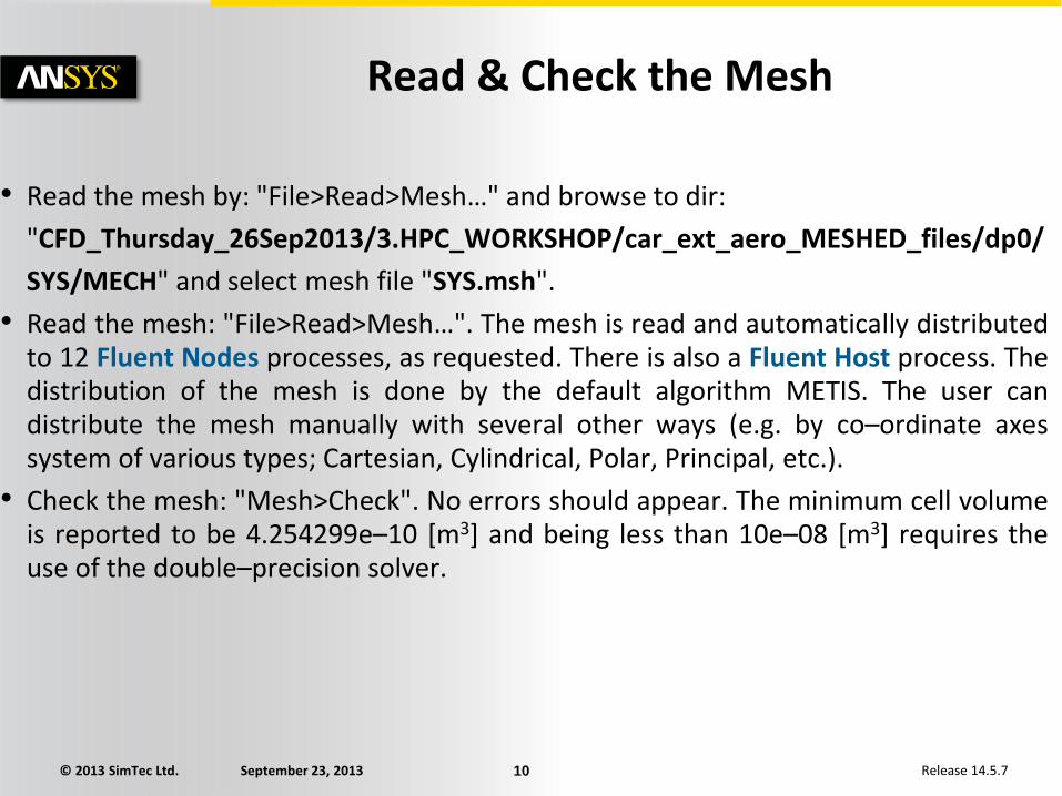
Read & Check the Mesh

• Read the mesh by: "File>Read>Mesh…" and browse to dir:

"CFD_Thursday_26Sep2013/3.HPC_WORKSHOP/car_ext_aero_MESHED_files/dp0/

SYS/MECH" and select mesh file "SYS.msh".

• Read the mesh: "File>Read>Mesh…". The mesh is read and automatically distributedto 12 Fluent Nodes processes, as requested. There is also a Fluent Host process. Thedistribution of the mesh is done by the default algorithm METIS. The user candistribute the mesh manually with several other ways (e.g. by co–ordinate axessystem of various types; Cartesian, Cylindrical, Polar, Principal, etc.).

• Check the mesh: "Mesh>Check". No errors should appear. The minimum cell volumeis reported to be 4.254299e–10 [m3] and being less than 10e–08 [m3] requires theuse of the double–precision solver.


• Activate turbulence modeling. In "Models" branch of the model tree at the left,select "Viscous – Laminar" and click button "Edit…". From the list select the k–om/SST 2–equation eddy–viscosity model, with the settings, as shown.

Turbulence Modeling


• Although the car is moving into stagnant air, it’s convenient from a computationalpoint of view to change the system of reference and assume a stationary car andflowing air.

• inlet: The air enters with a uniform profile of 50 [m/s] (=180 [km/h]), with mildturbulence level, as shown in the BC panel. We use the "Velocity Inlet" type of BC.

Boundary Conditions (BCs) – 1


• top & side: although there are other alternative BCs for the top boundary(symmetry), we will use the same settings as with "inlet" boundary. This is a goodapproximation, which also helps faster convergence, provided these boundaries arelocated remotely enough from the car (because essentially we are forcing the airflow to have a certain direction and velocity, whereas in reality this happens atinfinity from the body that deflects the flow away from it).

• In order to copy the "inlet" BC, we need first

to make them of the same type. Select "side" and

then "top" zones and in the "Type" list selecyt

"velocity–inlet".

• Now press button "Copy…" and then "inlet" from the list "From

Boundary Zone" and finally select "side" and

"top" from the list "To Boundary Zones".



• outlet: The air is expanding to atmospheric conditions away downstream the car.This is accomplished by a "Pressure Outlet" type of BC, as shown below. We areusing a zero gauge pressure, i.e. atmospheric pressure (see later for setting theoperating pressure). The "Backflow" settings for turbulence will only take effect ifbackflow will occur (the flow may not exit but may enter the domain from part ofthe boundary).



• walls & symmetry: All walls are stationary (remember the car is not moving; the airdoes), except the wheels which are rotating (see below) and need no specialtreatment. The default settings (stationary with no–slip condition is the right one).Also, symmetry plane needs no change.

• wheels: The two walls, corresponding to the two wheels (front & rear) should berotating with reference to the local wheel axis. The rotation speed is calculated bytranslating the linear velocity of the car to a rotating speed of the wheel with itsexternal diameter (85 [cm]).



• Operating Pressure: Press button "Operating Conditions…" (shown when the"Boundary Conditions" branch is selected) and set the "Operating Pressure" to101325 [Pa], which corresponds to the standard atmospheric conditions. So, thegauge pressure input and output is the difference from the atmospheric pressure of101325 [Pa].

Operating Conditions


• Select "Solution Methods" branch in the model tree and set the discretizationmethod as shown on the left.

• Then Select "Solution Controls" and set the Under–Relaxation Factors (URFs) asshown on the right.

Solution Settings & Controls


• Set convenient monitors to track convergence.

Cd for the car body.

Area–weighted turbulent kinetic energy at the "outlet" (wake of the body).

Volume–average pressure over the whole domain.

• Iterate.

Monitors & Iteration

Express Introductory Training in ANSYS Fluent be exported from ANSYS Meshing; the "Mesh" cell B2 to...

Documents

Transcript of Express Introductory Training in ANSYS Fluent be exported from ANSYS Meshing; the "Mesh" cell B2 to...