CFD basics & Use of ANSY FLUENT in Engineering Application: A Brief

Introduction Prepared by:MD SHUJAN ALI GTA for Aero-3Graduate Student Aerospace Engineering Auburn University Auburn, Alabama, USA

Fluid Dynamics• Fluid Dynamics is both interesting & challenging

field for study and research. In real world almost everywhere fluid is present. So, we need fluid dynamics to describe or model these fluid flows.

• In brief any fluid flow can be solved/Described by three basic physical law, or by three equations.(1)Continuity equation- Mass is conserved.(2)Momentum equation (Widely knows as Navier-Stokes equation)- Newton’s Second Law.(3)Energy equation- Energy is conserved.

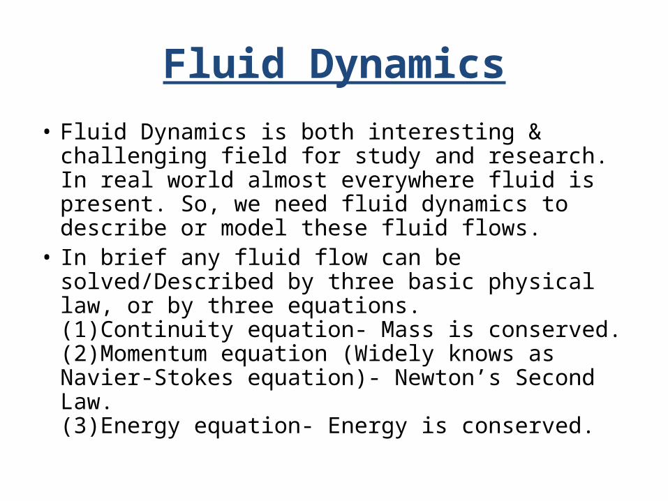
Three ways of solving problems Any problem/phenomena can be analyzed by three ways •Analytical/Theoretical approach- using laws/theories and associated equations, such as using Newton’s law of viscosity to solve a fluid flow problem, these solutions are exact.•Experimental approach- do experiments and try to understand the phenomena and relation between various variables, such as wind tunnel experiments which helps to design and optimize external shape of airplanes, ships, automobiles etc.•Numerical approach-Solve a fluid flow problem using numerical techniques. These solutions are approximate, not exact.

What is CFD

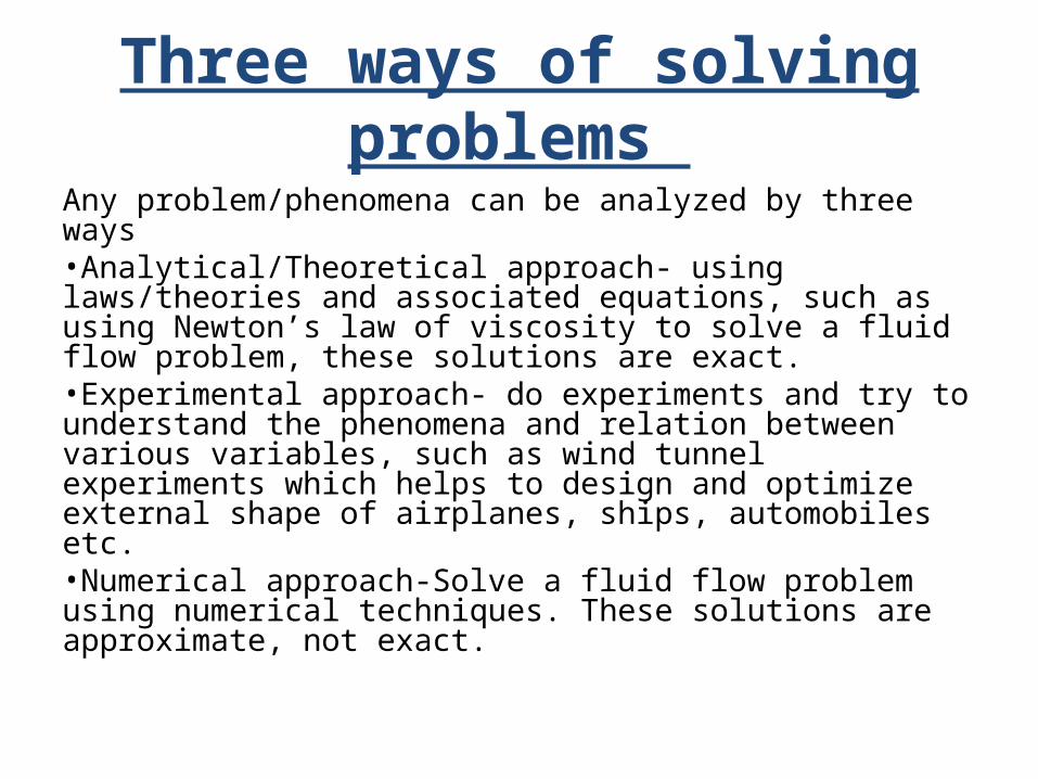
• Computational Fluid Dynamics (CFD) is a set of numerical methods applied to obtain approximate solutions of problems of fluid dynamics and heat transfer.

• So, CFD is not a science by itself, it is a way to apply the methods of one discipline (numerical analysis) to another (fluid flow/mass transfer and heat transfer).

Why CFD

• CFD solutions are not exact, then why not use Analytical approach???

• Experimental approach is more reliable, such as wind tunnel experiments, why not use experimental approach instead of CFD???

CFD is used because there are many engineering problems that can’t be solved by analytical or Experimental approach, or it is difficult to use analytical or experimental approach.

Difficulties in other approaches• Theoretical approach: This approach gives exact

solution which is a great advantage. But analytical solutions are only possible for a limited number of problems, usually formulated in an artificial, idealized way.

• Experimental approach: These approaches are reliable, and depict real world situations. For example, in aerospace industries Wind Tunnel experiments are very reliable. But some times these are very expensive, and some times these also have some technical difficulties (Sometimes it takes several years before an experiment is set up and all technical problems are resolved).

Application of CFDCFD is a very powerful technique and spans a wide a wide range of industrial and non-industrial applications. Some examples are –•Aerodynamics of aircrafts and vehicles: Drag & Lift •Power plant: Combustion in internal combustion engines & Gas turbines.•Hydrodynamics of ships •Biomedical engineering: Blood flow through arteries and veins •Environmental engineering: distribution of pollutants In a nutshell, CFD is applied in almost every disciplines of Engineering. From the 1960s onwards Aerospace industries has integrated CFD techniques in the design, R&D, and manufacturing of Aircrafts and Jet engines.

Own Coding vs Commercial CFD codes

CFD is solving basic equations of fluid flow and heat transfer by applying Numerical techniques. There are two different approach-(1)Write your own CFD code to solve a specific problem, or a type of problem. For example, you can write your own MATLAB program to solve a incompressible pipe flow. (2)There are some commercial CFD software package. Some of them are very puseful & popular. Example: ANSYS FLUENT, STAR-CD, CFX, OpenFOAM, and COMSOL.

Problem solving using commercial CFD packages

CFD codes are structured around the numerical algorithms that can tackle fluid flow problems. In order to provide easy access to their solving power all commercial CFD packages include sophisticated user interfaces to input problem parameters and to examine the results. Hence all codes contain three main elements: (i) a pre-processor, (ii) a solver and (iii) a post processor.Pre-processor: This step includes creating Geometry and Mesh. Solver: This part is to numerically solve the fluid flow equations in the computational domain.Post-Processor: In this steps, result of simulation is analyzed, or represented in useful form. In ANSYS WORKBENCH, Design Modeler & Meshing works as pre-processor, FLUENT is the Solver, and CFD-post is the post-processor.

Three methods of CFD

There are three basic methods to solve problem in CFD.(1)Finite difference method (2)Finite element method(3) Spectral methods Finite Volume Method is a special case of Finite difference method. It is a very popular method.

ANSY FLUENT ANSYS, Inc. is an engineering simulation software (computer-aided engineering, or CAE) developer headquartered south of Pittsburgh in the Southpointe business park in Cecil Township, Pennsylvania, United States. One of its most significant products is Ansys CFD, a proprietary computational fluid dynamics (CFD) program (Source-Wikipedia). ANSYS FLUENT is one of the most popular commercial CFD software packages. We will use ANSYS FLUENT in this course to solve Engineering problems.

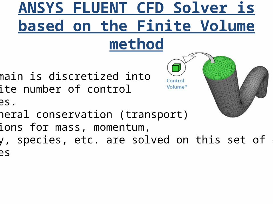
ANSYS FLUENT CFD Solver is based on the Finite Volume method

***Domain is discretized intoa finite number of control volumes.***General conservation (transport) equations for mass, momentum, energy, species, etc. are solved on this set of control volumes

Steps solving problem by ANSYS FLUENT

To solve Engineering problems using ANSYS FLUENT the necessary steps are-(1)Pre-analysis(2)Geometry(3)Mesh(4)Physical Setup(5)Numerical Solution(6)Verification & Validation

ANSYS WORKBENCH

ANSYS WORKBENCH is a Graphical User Interface(GUI) that allows the user to use all the required tools/software from a single place. You can access pre-processor, solver and post-processor tools from ANSYS WORKBENCH. You will control your workflow between various tools through Workbench.

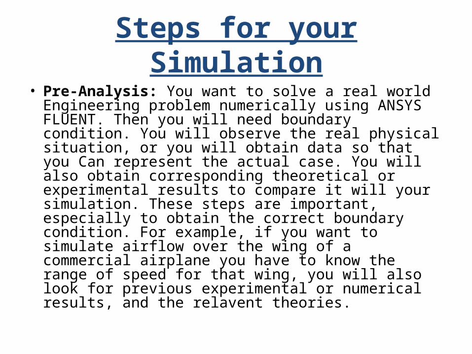
Steps for your Simulation• Pre-Analysis: You want to solve a real world Engineering

problem numerically using ANSYS FLUENT. Then you will need boundary condition. You will observe the real physical situation, or you will obtain data so that you Can represent the actual case. You will also obtain corresponding theoretical or experimental results to compare it will your simulation. These steps are important, especially to obtain the correct boundary condition. For example, if you want to simulate airflow over the wing of a commercial airplane you have to know the range of speed for that wing, you will also look for previous experimental or numerical results, and the relavent theories.

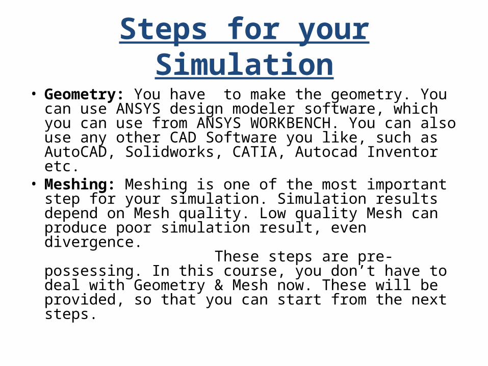
Steps for your Simulation• Geometry: You have to make the geometry. You can

use ANSYS design modeler software, which you can use from ANSYS WORKBENCH. You can also use any other CAD Software you like, such as AutoCAD, Solidworks, CATIA, Autocad Inventor etc.

• Meshing: Meshing is one of the most important step for your simulation. Simulation results depend on Mesh quality. Low quality Mesh can produce poor simulation result, even divergence. These steps are pre-possessing. In this course, you don’t have to deal with Geometry & Mesh now. These will be provided, so that you can start from the next steps.

Steps for your Simulation

• Physical Setup: It is done in the solver ANSYS. Your concentration will be to understand and perform physical setup, numerical result, and Verification & Validation. In physical setup step, you give inputs for solution accuracy, boundary condition, physics involved, material involved, properties of involved etc. In a nutshell, here you numerically depict the real situation you want to simulate.

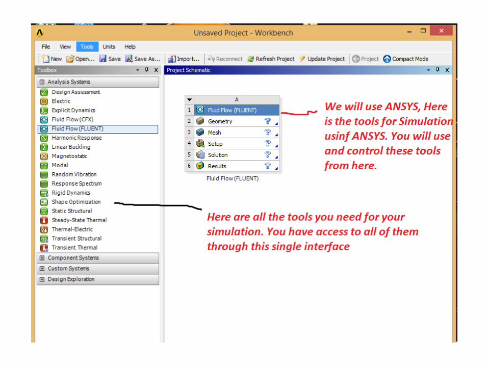
Starting ANSYS• ANSYS WORKBENCH >>> Analysis systems >>> Fluid

Flow(FLUENT) you will state FLUENT solver using this path. FLUENT tree will appear which looks like

This tree showing the all the steps you have to complete for a successfulsimulation. Now you can skip Geometry & Meshing. You will start from Setup tab which is physical setup.

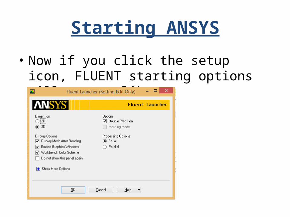
Starting ANSYS

• Now if you click the setup icon, FLUENT starting options will appear like

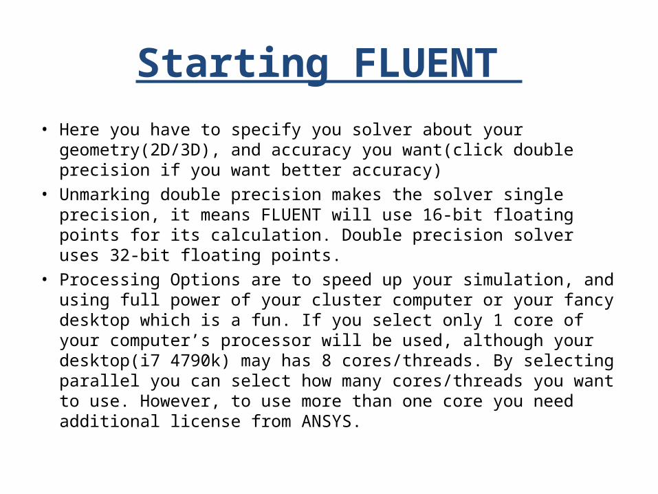
Starting FLUENT • Here you have to specify you solver about your geometry(2D/3D),

and accuracy you want(click double precision if you want better accuracy)

• Unmarking double precision makes the solver single precision, it means FLUENT will use 16-bit floating points for its calculation. Double precision solver uses 32-bit floating points.

• Processing Options are to speed up your simulation, and using full power of your cluster computer or your fancy desktop which is a fun. If you select only 1 core of your computer’s processor will be used, although your desktop(i7 4790k) may has 8 cores/threads. By selecting parallel you can select how many cores/threads you want to use. However, to use more than one core you need additional license from ANSYS.

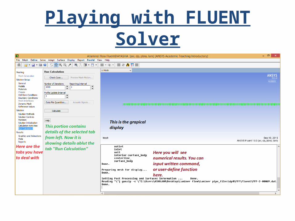
Playing with FLUENT Solver

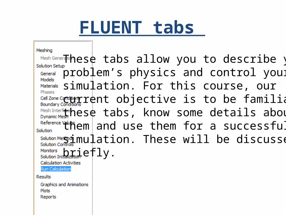
FLUENT tabs

These tabs allow you to describe yourproblem’s physics and control your simulation. For this course, our current objective is to be familiar with these tabs, know some details about them and use them for a successful simulation. These will be discussedbriefly.

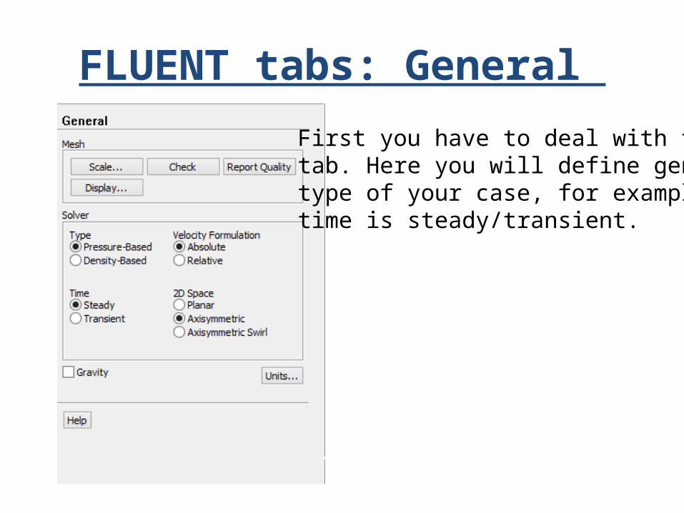
FLUENT tabs: General First you have to deal with this tab. Here you will define generaltype of your case, for exampletime is steady/transient.

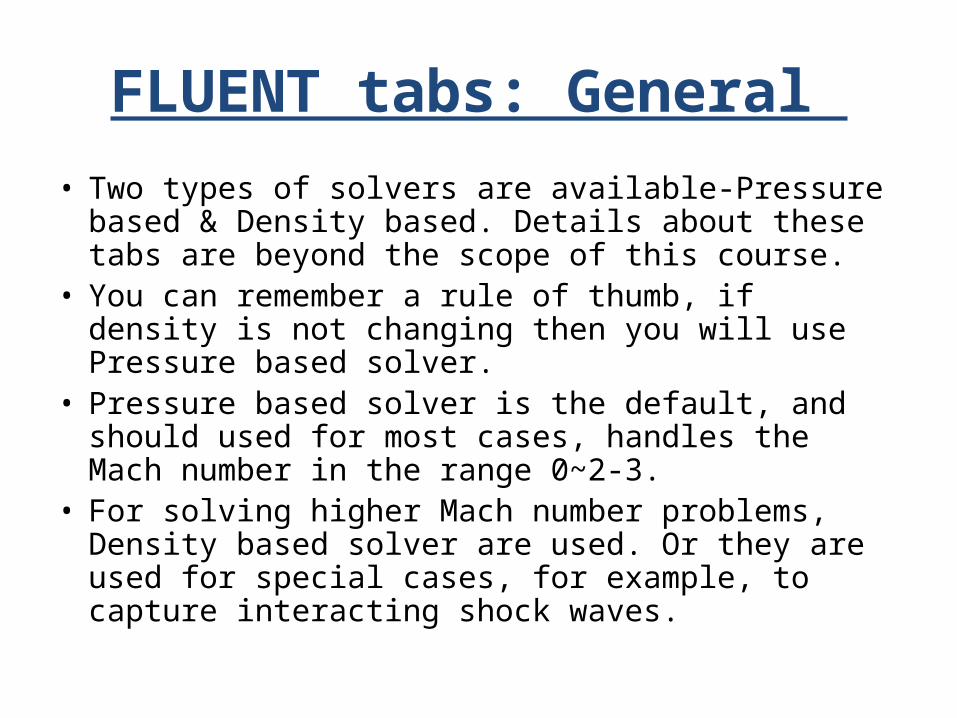
FLUENT tabs: General • Two types of solvers are available-Pressure based &

Density based. Details about these tabs are beyond the scope of this course.

• You can remember a rule of thumb, if density is not changing then you will use Pressure based solver.

• Pressure based solver is the default, and should used for most cases, handles the Mach number in the range 0~2-3.

• For solving higher Mach number problems, Density based solver are used. Or they are used for special cases, for example, to capture interacting shock waves.

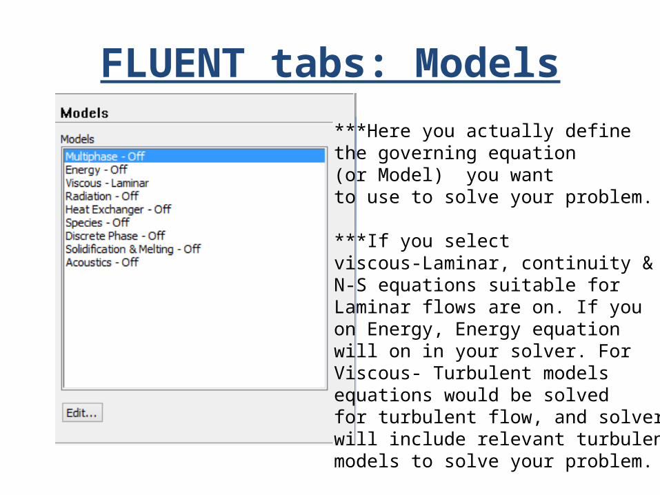
FLUENT tabs: Models***Here you actually define the governing equation (or Model) you want to use to solve your problem.

***If you select viscous-Laminar, continuity & N-S equations suitable for Laminar flows are on. If youon Energy, Energy equationwill on in your solver. For Viscous- Turbulent models equations would be solved for turbulent flow, and solver will include relevant turbulentmodels to solve your problem.

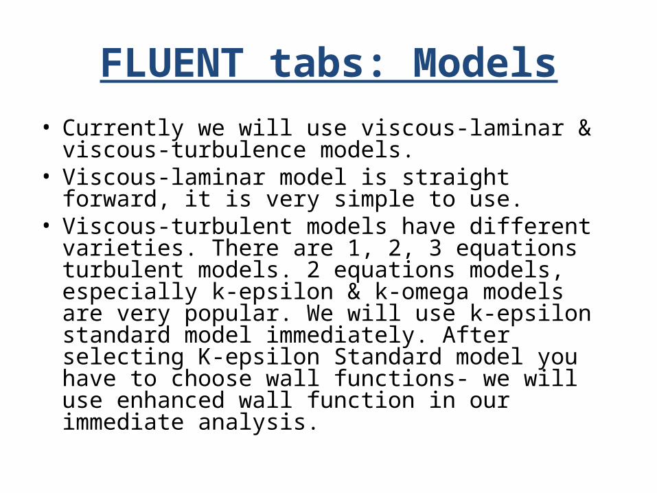
FLUENT tabs: Models• Currently we will use viscous-laminar & viscous-

turbulence models.• Viscous-laminar model is straight forward, it is very

simple to use. • Viscous-turbulent models have different varieties.

There are 1, 2, 3 equations turbulent models. 2 equations models, especially k-epsilon & k-omega models are very popular. We will use k-epsilon standard model immediately. After selecting K-epsilon Standard model you have to choose wall functions- we will use enhanced wall function in our immediate analysis.

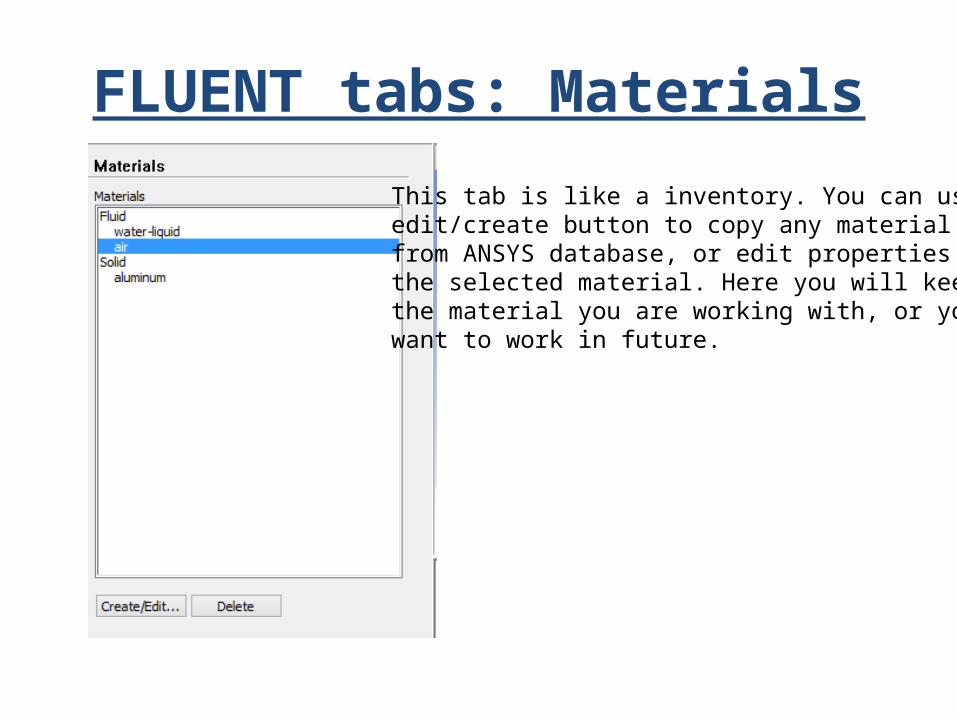
FLUENT tabs: MaterialsThis tab is like a inventory. You can use the edit/create button to copy any material from ANSYS database, or edit properties of the selected material. Here you will keep all the material you are working with, or you want to work in future.

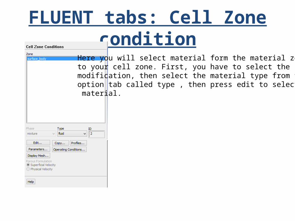
FLUENT tabs: Cell Zone conditionHere you will select material form the material zone,to your cell zone. First, you have to select the zone for modification, then select the material type from the option tab called type , then press edit to select the material.

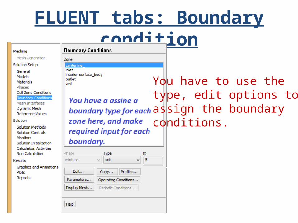
FLUENT tabs: Boundary condition

You have to use the type, edit options to assign the boundary conditions.

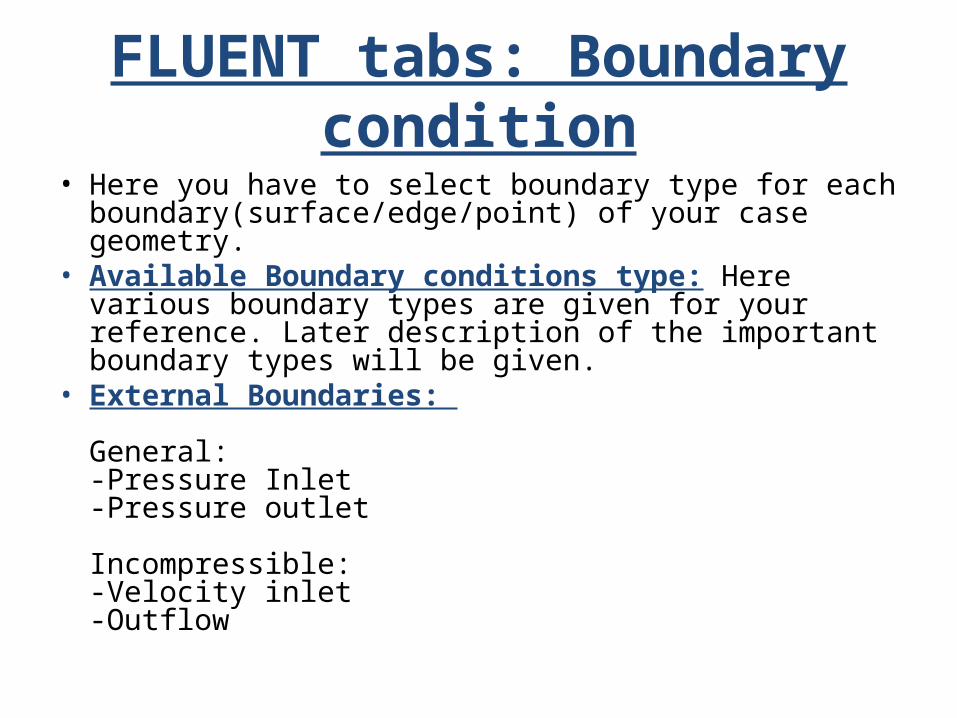
FLUENT tabs: Boundary condition• Here you have to select boundary type for each

boundary(surface/edge/point) of your case geometry. • Available Boundary conditions type: Here various

boundary types are given for your reference. Later description of the important boundary types will be given.

• External Boundaries:

General: -Pressure Inlet -Pressure outlet

Incompressible:-Velocity inlet-Outflow

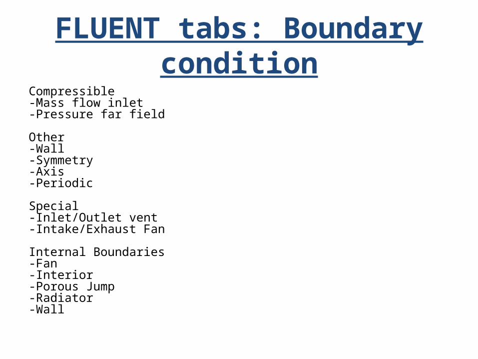
FLUENT tabs: Boundary conditionCompressible-Mass flow inlet -Pressure far field

Other -Wall-Symmetry -Axis-Periodic

Special-Inlet/Outlet vent -Intake/Exhaust Fan

Internal Boundaries-Fan -Interior -Porous Jump -Radiator -Wall

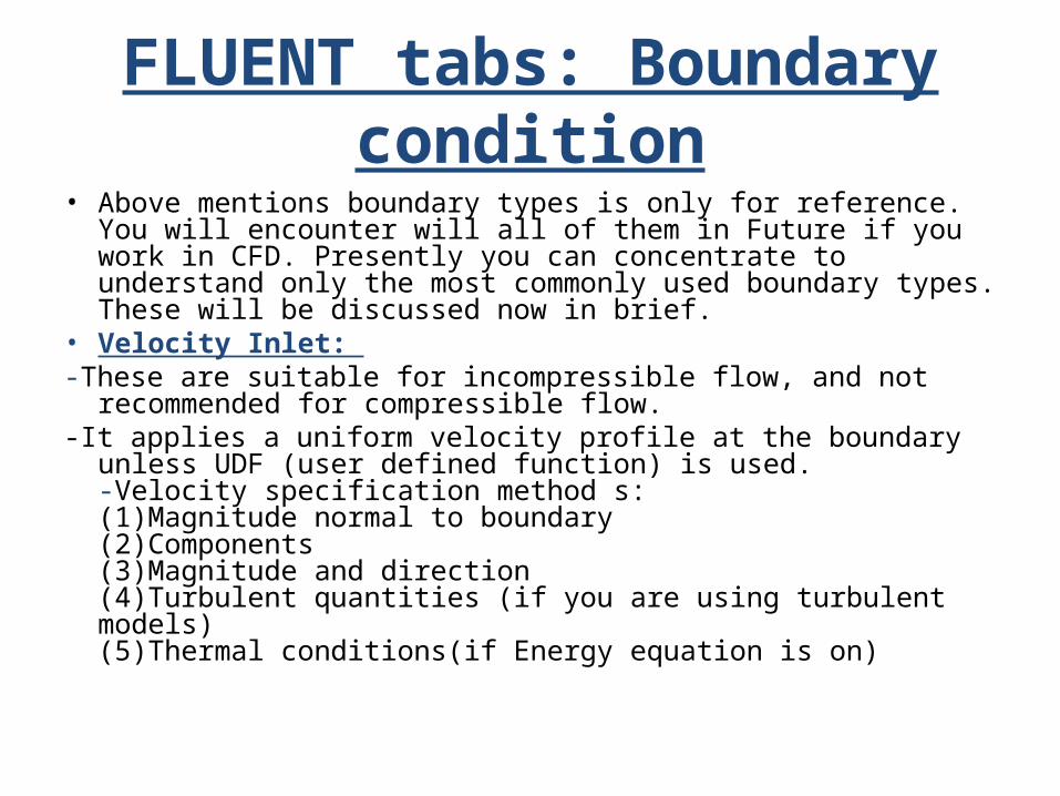
FLUENT tabs: Boundary condition• Above mentions boundary types is only for reference. You will

encounter will all of them in Future if you work in CFD. Presently you can concentrate to understand only the most commonly used boundary types. These will be discussed now in brief.

• Velocity Inlet: -These are suitable for incompressible flow, and not recommended for

compressible flow.-It applies a uniform velocity profile at the boundary unless UDF (user

defined function) is used.-Velocity specification method s:(1)Magnitude normal to boundary (2)Components (3)Magnitude and direction(4)Turbulent quantities (if you are using turbulent models) (5)Thermal conditions(if Energy equation is on)

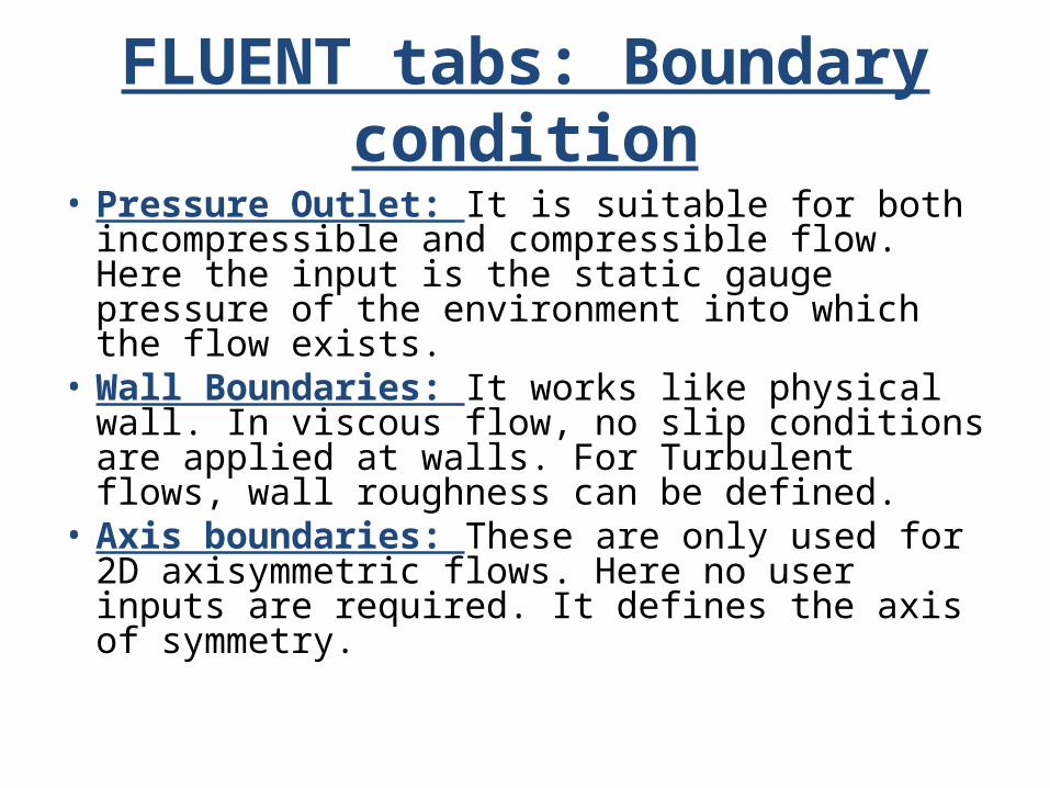
FLUENT tabs: Boundary condition• Pressure Outlet: It is suitable for both

incompressible and compressible flow. Here the input is the static gauge pressure of the environment into which the flow exists.

• Wall Boundaries: It works like physical wall. In viscous flow, no slip conditions are applied at walls. For Turbulent flows, wall roughness can be defined.

• Axis boundaries: These are only used for 2D axisymmetric flows. Here no user inputs are required. It defines the axis of symmetry.

FLUENT tabs: Dynamic Mesh

• You can ship this step now. It is used only for simulating moving objects, such as for simulation a moving turbine blade.

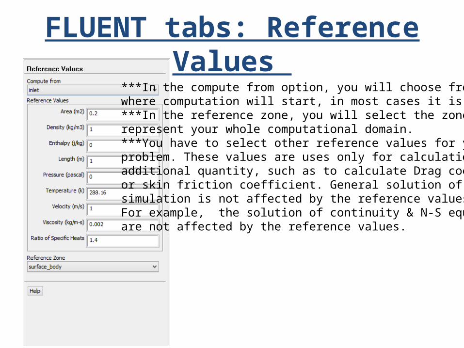
FLUENT tabs: Reference Values ***In the compute from option, you will choose from where computation will start, in most cases it is the inlet.***In the reference zone, you will select the zone that represent your whole computational domain. ***You have to select other reference values for your problem. These values are uses only for calculation someadditional quantity, such as to calculate Drag coefficient, or skin friction coefficient. General solution of the simulation is not affected by the reference values. For example, the solution of continuity & N-S equations are not affected by the reference values.

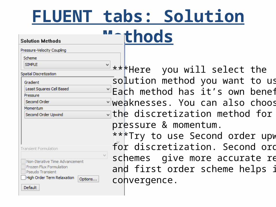
FLUENT tabs: Solution Methods

***Here you will select the solution method you want to use. Each method has it’s own benefit & weaknesses. You can also choose the discretization method forpressure & momentum. ***Try to use Second order upwind for discretization. Second order schemes give more accurate result,and first order scheme helps in convergence.

FLUENT tabs: Solution Methods

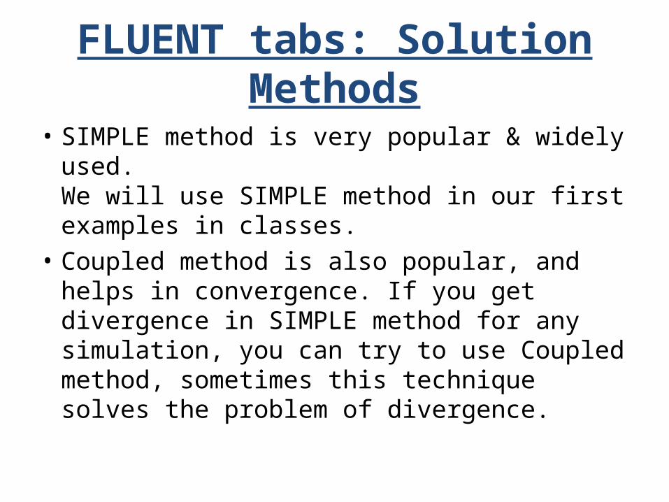
• SIMPLE method is very popular & widely used. We will use SIMPLE method in our first examples in classes.

• Coupled method is also popular, and helps in convergence. If you get divergence in SIMPLE method for any simulation, you can try to use Coupled method, sometimes this technique solves the problem of divergence.

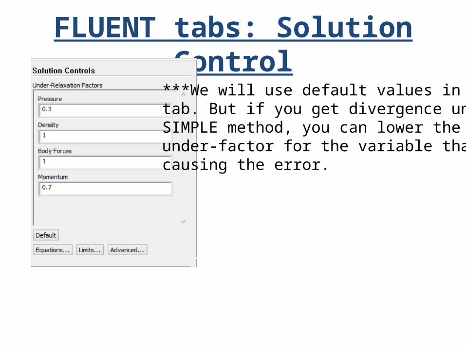
FLUENT tabs: Solution Control***We will use default values in this tab. But if you get divergence under SIMPLE method, you can lower the under-factor for the variable that causing the error.

FLUENT tabs: Solution Monitors

FLUENT tabs: Solution Control

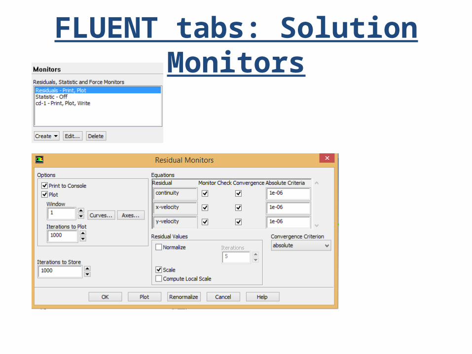
• Here you can monitor your simulation. In the residual monitor you can select the level of floating point accuracy you want. You can add additional monitors for additional properties. For example, you can add additional monitors to plot drag coefficient, lift coefficient, momentum coefficient. We will demonstrate these in classes.

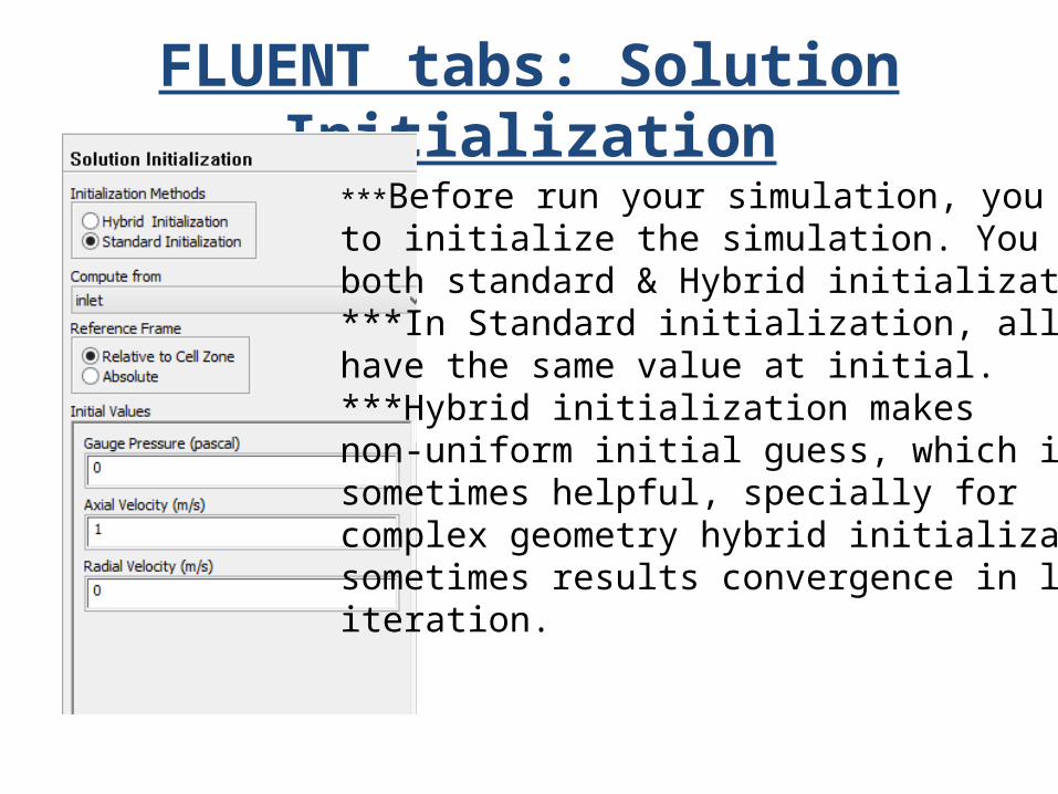
FLUENT tabs: Solution Initialization***Before run your simulation, you haveto initialize the simulation. You can both standard & Hybrid initialization. ***In Standard initialization, all cells have the same value at initial.***Hybrid initialization makes non-uniform initial guess, which is sometimes helpful, specially for complex geometry hybrid initialization sometimes results convergence in less iteration.

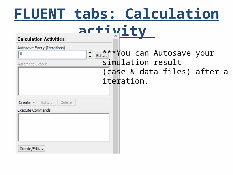
FLUENT tabs: Calculation activity

***You can Autosave your simulation result (case & data files) after a fixed iteration.

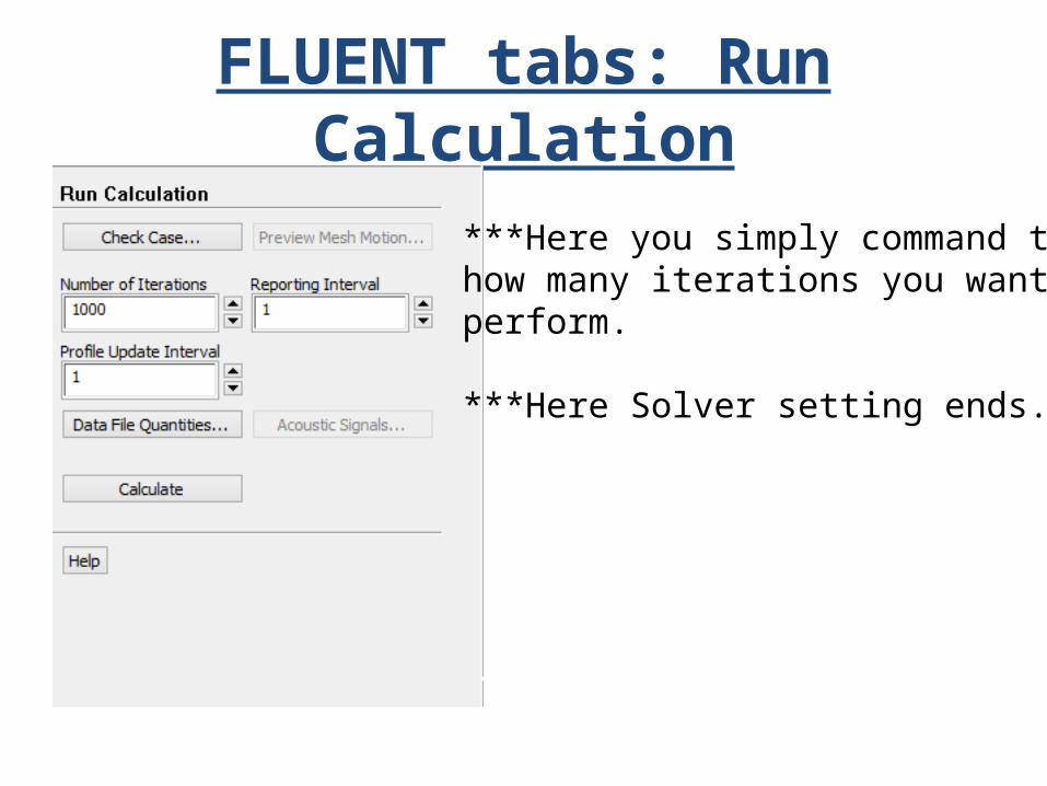
FLUENT tabs: Run Calculation

***Here you simply command that how many iterations you want to perform.

***Here Solver setting ends.

Next Steps • The steps are post processing, i.e., analyzing your

simulation results and data, and verification.• We will use CFD-post for post processing. We can

also use FLUENT solver for post-processing, but CFD-post is easier & convenient.

• We want to verify whether or not our simulation is correct? For verification, we can check whether basic physical laws are maintained or not, using FLUENT. For example, we can check that, does our solution satisfy continuity equation? We will see details about it in class.

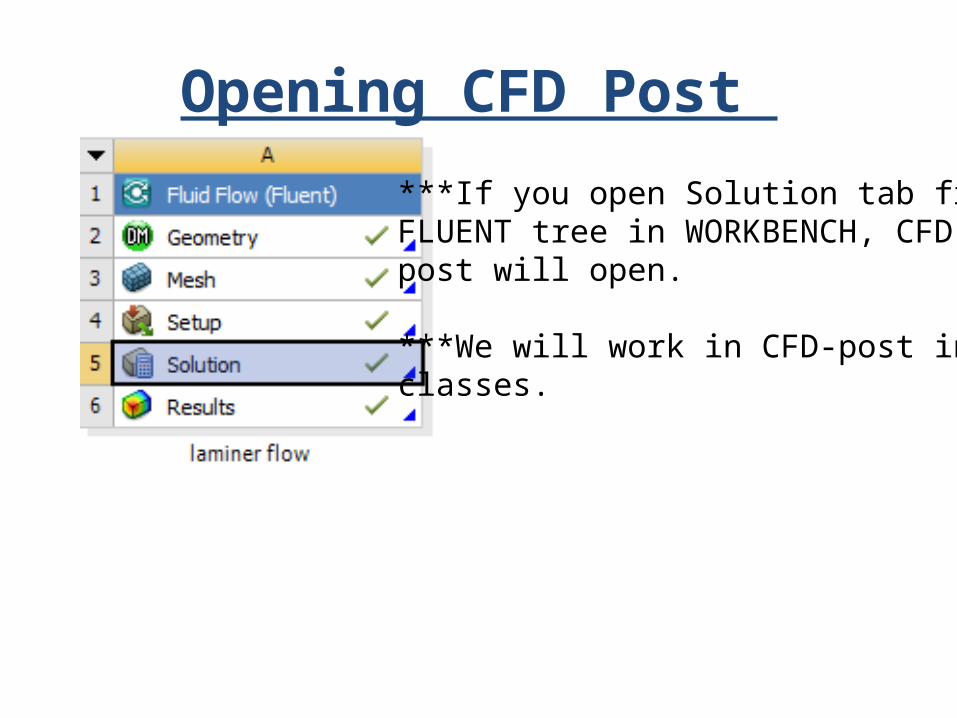
Opening CFD Post ***If you open Solution tab from FLUENT tree in WORKBENCH, CFD post will open.

***We will work in CFD-post in classes.

Notes • I try to make this slide as a quick & easy tutorial. You

will be familiar with CFD & ANSYS FLUENT by using this slide. If you try to run ANSYS FLUENT by yourself, you will be able to understand most of the things.

• We will do complete simulation step by step in class, then you will get the full picture.

• Next you can contact me if you have confusion, or want to know more. You can contact me in my office at Room-323 in my office time : Tuesday & Thursday- 11:30am-1:30pmWednesday-10:30pm-1:30pm

References• FLUENT Help, User’s guide, Theory Guide.• http://www.ansys.com/Products/

Simulation+Technology/Fluid+Dynamics/Fluid+Dynamics+Products/ANSYS+Fluent

• https://www.youtube.com/channel/UCdymxOTZSP8RzRgFT8kpYpA

• http://www.ansys.com/Industries/Academic/Student+Product/Product+Information

• An Introduction to Computational Fluid Dynamics-THE FINITE VOLUME METHOD, Second Edition, H K Versteeg and W Malalasekera

References

• ESSENTIAL COMPUTATIONAL FLUID DYNAMICS, OLEZ ZIKANOV