Meta-Gradient Reinforcement Learning

Zhongwen XuDeepMind

zhongwen@google.com

Hado van HasseltDeepMind

hado@google.com

David SilverDeepMind

davidsilver@google.com

Abstract

The goal of reinforcement learning algorithms is to estimate and/or optimisethe value function. However, unlike supervised learning, no teacher or oracle isavailable to provide the true value function. Instead, the majority of reinforcementlearning algorithms estimate and/or optimise a proxy for the value function. Thisproxy is typically based on a sampled and bootstrapped approximation to the truevalue function, known as a return. The particular choice of return is one of thechief components determining the nature of the algorithm: the rate at which futurerewards are discounted; when and how values should be bootstrapped; or even thenature of the rewards themselves. It is well-known that these decisions are crucialto the overall success of RL algorithms. We discuss a gradient-based meta-learningalgorithm that is able to adapt the nature of the return, online, whilst interactingand learning from the environment. When applied to 57 games on the Atari 2600environment over 200 million frames, our algorithm achieved a new state-of-the-artperformance.

The central goal of reinforcement learning (RL) is to optimise the agent’s return (cumulative reward);this is typically achieved by a combination of prediction and control. The prediction subtask is toestimate the value function – the expected return from any given state. Ideally, this would be achievedby updating an approximate value function towards the true value function. The control subtask is tooptimise the agent’s policy for selecting actions, so as to maximise the value function. Ideally, thepolicy would simply be updated in the direction that increases the true value function. However, thetrue value function is unknown and therefore, for both prediction and control, a sampled return isinstead used as a proxy. A large family of RL algorithms [Sutton, 1988, Rummery and Niranjan,1994, van Seijen et al., 2009, Sutton and Barto, 2018], including several state-of-the-art deep RLalgorithms [Mnih et al., 2015, van Hasselt et al., 2016, Harutyunyan et al., 2016, Hessel et al., 2018,Espeholt et al., 2018], are characterised by different choices of the return.

The discount factor γ determines the time-scale of the return. A discount factor close to γ = 1provides a long-sighted goal that accumulates rewards far into the future, while a discount factorclose to γ = 0 provides a short-sighted goal that prioritises short-term rewards. Even in problemswhere long-sightedness is clearly desired, it is frequently observed that discounts γ < 1 achievebetter results [Prokhorov and Wunsch, 1997], especially during early learning. It is known that manyalgorithms converge faster with lower discounts [Bertsekas and Tsitsiklis, 1996], but of course toolow a discount can lead to highly sub-optimal policies that are too myopic. In practice it can be betterto first optimise for a myopic horizon, e.g., with γ = 0 at first, and then to repeatedly increase thediscount only after learning is somewhat successful [Prokhorov and Wunsch, 1997].

The return may also be bootstrapped at different time horizons. An n-step return accumulates rewardsover n time-steps and then adds the value function at the nth time-step. The λ-return [Sutton, 1988,Sutton and Barto, 2018] is a geometrically weighted combination of n-step returns. In either case,the meta-parameter n or λ can be important to the performance of the algorithm, trading off bias andvariance. Many researchers have sought to automate the selection of these parameters [Kearns andSingh, 2000, Downey and Sanner, 2010, Konidaris et al., 2011, White and White, 2016].

32nd Conference on Neural Information Processing Systems (NeurIPS 2018), Montréal, Canada.

There are potentially many other design choices that may be represented in the return, includingoff-policy corrections [Espeholt et al., 2018, Munos et al., 2016], target networks [Mnih et al., 2015],emphasis on certain states [Sutton et al., 2016], reward clipping [Mnih et al., 2013], or even the natureof the rewards themselves [Randløv and Alstrøm, 1998, Singh et al., 2005, Zheng et al., 2018].

In this work, we are interested in one of the fundamental problems in reinforcement learning: whatwould be the best form of return for the agent to maximise? Specifically, we propose to learn thereturn function by treating it as a parametric function with tunable meta-parameters η, for instanceincluding the discount factor γ, or the bootstrapping parameter λ [Sutton, 1988]. The meta-parametersη are adjusted online during the agent’s interaction with the environment, allowing the return toboth adapt to the specific problem, and also to dynamically adapt over time to the changing contextof learning. We derive a practical gradient-based meta-learning algorithm and show that this cansignificantly improve performance on large-scale deep reinforcement learning applications.

1 Meta-Gradient Reinforcement Learning Algorithms

In deep reinforcement learning, the value function and policy are approximated by a neural networkwith parameters θ, denoted by vθ(S) and πθ(A|S) respectively. At the core of the algorithm is anupdate function,

θ′ = θ + f(τ, θ, η) , (1)

that adjusts parameters from a sequence of experience τt = {St, At, Rt+1, . . .} consisting of statesS, actions A and rewards R. The nature of the function is determined by meta-parameters η.

Our meta-gradient RL approach is based on the principle of online cross-validation [Sutton, 1992],using successive samples of experience. The underlying RL algorithm is applied to the first sample(or samples), and its performance is measured in a subsequent sample. Specifically, the algorithmstarts with parameters θ, and applies the update function to the first sample(s), resulting in newparameters θ′. The gradient dθ′/dη of these updates indicates how the meta-parameters affectedthese new parameters.

The algorithm then measures the performance of the new parameters θ′ on a second sample τ ′. Forinstance, when learning online τ ′ could be the next time-step immediately following τ . Performanceis measured by a differentiable meta-objective J̄(τ ′, θ′, η̄) that uses a fixed meta-parameter η̄.

The gradient of the meta-objective with respect to the meta-parameters η is obtained by applying thechain rule:

∂J̄(τ ′, θ′, η̄)

∂η=∂J̄(τ ′, θ′, η̄)

∂θ′dθ′

dη. (2)

To compute the gradient of the updates, dθ′/dη, we note that the parameters form an additive sequence,and the gradient can therefore be accumulated online [Williams and Zipser, 1989],

dθ′

dη=

dθdη

+∂f(τ, θ, η)

∂η+∂f(τ, θ, η)

∂θ

dθdη

=

(I +

∂f(τ, θ, η)

∂θ

)dθdη

+∂f(τ, θ, η)

∂η(3)

This update has the form

z′ = Az +∂f(τ, θ, η)

∂η,

where z = dθ/dη and z′ = dθ′/dη.

The exact gradient is given by A = I + ∂f(τ, θ, η)/∂θ. In practice, the gradient ∂f(τ, θ, η)/∂θ islarge and challenging to compute — it is a n× n matrix, where n is the number of parameters in θ.In practice, we approximate the gradient, z ≈ dθ/dη. One possibility is to use an alternate updateA = I + ∂̂f(τ, θ, η)/∂̂θ using a cheap approximate derivative ∂̂f(τ, θ, η)/∂̂θ ≈ ∂f(τ, θ, η)/∂θ,for instance using a diagonal approximation [Sutton, 1992, Schraudolph, 1999]. Furthermore, thegradient accumulation defined above assumes that the meta-parameters η are held fixed throughouttraining. In practice, we are updating η and therefore it may be desirable to decay the trace into thepast [Schraudolph, 1999], A = µ(I + ∂f(τ, θ, η)/∂θ), using decay rate µ ∈ [0, 1]. The simplestapproximation is to use A = 0 (or equivalently µ = 0), which means that we only consider the effectof the meta-parameters η on a single update; this approximation is especially cheap to compute.

2

Finally, the meta-parameters η are updated to optimise the meta-objective, for example by applyingstochastic gradient descent (SGD) to update η in the direction of the meta-gradient,

∆η = −β ∂J̄(τ ′, θ′, η̄)

∂θ′z′, (4)

where β is the learning rate for updating meta parameter η. The pseudo-code for the meta-gradientreinforcement learning algorithm is provided in Appendix A.

In the following sections we instantiate this idea more specifically to RL algorithms based onpredicting or controlling returns. We begin with a pedagogical example of using meta-gradients forprediction using a temporal-difference update. We then consider meta-gradients for control, using acanonical actor-critic update function and a policy gradient meta-objective. Many other instantiationsof meta-gradient RL would be possible, since the majority of deep reinforcement learning updates aredifferentiable functions of the return, including, for instance, value-based methods like SARSA(λ)[Rummery and Niranjan, 1994, Sutton and Barto, 2018] and DQN [Mnih et al., 2015], policy-gradient methods [Williams, 1992], or actor-critic algorithms like A3C [Mnih et al., 2016] andIMPALA [Espeholt et al., 2018].

1.1 Applying Meta-Gradients to Returns

We define the return gη(τt) to be a function of an episode or a truncated n-step sequence of experienceτt = {St, At, Rt+1, . . . , St+n}. The nature of the return is determined by the meta-parameters η.

The n-step return [Sutton and Barto, 2018] accumulates rewards over the sequence and then bootstrapsfrom the value function,

gη(τt) = Rt+1 + γRt+2 + γ2Rt+3 + . . . ,+γn−1Rt+n + γnvθ(St+n) (5)

where η = {γ}.The λ-return is a geometric mixture of n-step returns, [Sutton, 1988]

gη(τt) = Rt+1 + γ(1− λ)vθ(St+1) + γλgη(τt+1) (6)

where η = {γ, λ}. The λ-return has the advantage of being fully differentiable with respect to themeta-parameters. The meta-parameters η may be viewed as gates that cause the return to terminate(γ = 0) or bootstrap (λ = 0), or to continue onto the next step (γ = 1 and λ = 1). The n-stepor λ-return can be augmented with off-policy corrections [Precup et al., 2000, Sutton et al., 2014,Espeholt et al., 2018] if it is necessary to correct for the distribution used to generate the data.

A typical RL algorithm would hand-select the meta-parameters, such as the discount factor γ andbootstrapping parameter λ, and these would be held fixed throughout training. Instead, we view thereturn g as a function parameterised by meta-parameters η, which may be differentiated to understandits dependence on η. This in turn allows us to compute the gradient ∂f/∂η of the update functionwith respect to the meta-parameters η, and hence the meta-gradient ∂J̄(τ ′, θ′, η̄)/∂η. In essence,our agent asks itself the question, “which return results in the best performance?", and adjusts itsmeta-parameters accordingly.

1.2 Meta-Gradient Prediction

We begin with a simple instantiation of the idea, based on the canonical TD(λ) algorithm for prediction.The objective of the TD(λ) algorithm (according to the forward view [Sutton and Barto, 2018]) is tominimise the squared error between the value function approximator vθ(S) and the λ-return gη(τ),

J(τ, θ, η) = (gη(τ)− vθ(S))2 ∂J(τ, θ, η)

∂θ= −2(gη(τ)− vθ(S))

∂vθ(S)

∂θ(7)

where τ is a sampled trajectory starting with state S, and ∂J(τ, θ, η)/∂θ is a semi-gradient [Suttonand Barto, 2018], i.e. the λ-return is treated as constant with respect to θ.

The TD(λ) update function f(·) applies SGD to update the agent’s parameters θ to descend thegradient of the objective with respect to the parameters,

f(τ, θ, η) = −α2

∂J(τ, θ, η)

∂θ= α(gη(τ)− vθ(S))

∂vθ(S)

∂θ(8)

3

where α is the learning rate for updating agent θ. We note that this update is itself a differentiablefunction of the meta-parameters η,

∂f(τ, θ, η)

∂η= −α

2

∂2J(τ, θ, η)

∂θ ∂η= α

∂gη(τ)

∂η

∂vθ(S)

∂θ(9)

The key idea of the meta-gradient prediction algorithm is to adjust meta-parameters η in the directionthat achieves the best predictive accuracy. This is measured by cross-validating the new parameters θ′on a second trajectory τ ′ that starts from state S′, using a mean squared error (MSE) meta-objectiveand taking its semi-gradient,

J̄(τ ′, θ′, η̄) = (gη̄(τ ′)− vθ′(S′))2 ∂J̄(τ ′, θ′, η̄)

∂θ′= −2(gη̄(τ ′)− vθ′(S′))

∂vθ′(S′)

∂θ′(10)

The meta-objective in this case could make use of an unbiased and long-sighted return1, for exampleusing η̄ = {γ̄, λ̄} where γ̄ = 1 and λ̄ = 1.

1.3 Meta-Gradient Control

We now provide a practical example of meta-gradients applied to control. We focus on the A2Calgorithm – an actor-critic update function that combines both prediction and control into a singleupdate. This update function is widely used in several state-of-the-art agents [Mnih et al., 2016, Jader-berg et al., 2017b, Espeholt et al., 2018]. The semi-gradient of the A2C objective, ∂J(τ ; θ, η)/∂θ, isdefined as follows,

−∂J(τ, θ, η)

∂θ= (gη(τ)−vθ(S))

∂log πθ(A|S)

∂θ+b(gη(τ)−vθ(S))

∂vθ(S)

∂θ+c

∂H(πθ(·|S))

∂θ. (11)

The first term represents a control objective, encouraging the policy πθ to select actions that maximisethe return. The second term represents a prediction objective, encouraging the value functionapproximator vθ to more accurately estimate the return gη(τ). The third term regularises the policyaccording to its entropy H(πθ), and b, c are scalar coefficients that weight the different componentsin the objective function.

The A2C update function f(·) applies SGD to update the agent’s parameters θ. This update functionis a differentiable function of the meta-parameters η,

f(τ, θ, η) = −α∂J(τ, θ, η)

∂θ

∂f(τ, θ, η)

∂η= α

∂gη(τ)

∂η

[∂log πθ(A|S)

∂θ+ b

∂vθ(S)

∂θ

](12)

Now we come to the choice of meta-objective J̄ to use for control. Our goal is to identify the returnfunction that maximises overall performance in our agents. This may be directly measured by ameta-objective focused exclusively on optimising returns – in other words a policy gradient objective,

∂J̄(τ ′, θ′, η̄)

∂θ′= (gη̄(τ ′)− vθ′(S′))

∂log πθ′(A′|S′)

∂θ′. (13)

This equation evaluates how good the updated policy θ′ is in terms of returns computed under η̄, whenmeasured on “held-out” experiences τ ′, e.g. the subsequent n-step trajectory. When cross-validatingperformance using this meta-objective, we use fixed meta-parameters η̄, ideally representing a goodproxy to the true objective of the agent. In practice this typically means selecting reasonable values ofη̄; the agent is free to adapt its meta-parameters η and choose values that perform better in practice.

We now put the meta-gradient control algorithm together. First, the parameters θ are updated ona sample of experience τ using the A2C update function (Equation (11)), and the gradient of theupdate (Equation (12)) is accumulated into trace z. Second, the performance is cross-validated on asubsequent sample of experience τ ′ using the policy gradient meta-objective (Equation (13)). Finally,the meta-parameters η are updated according to the gradient of the meta-objective (Equation (4)).

1The meta-objective could even use a discount factor that is longer-sighted than the original problem, perhapsspanning over many episodes.

4

1.4 Conditioned Value and Policy Functions

One complication of the approach outlined above is that the return function gη(τ) is non-stationary,adapting along with the meta-parameters throughout the training process. As a result, there is adanger that the value function vθ becomes inaccurate, since it may be approximating old returns.For example, the value function may initially form a good approximation of a short-sighted returnwith γ = 0, but if γ subsequently adapts to γ = 1 then the value function may suddenly find itsapproximation is rather poor. The same principle applies for the policy π, which again may havespecialised to old returns.

To deal with non-stationarity in the value function and policy, we utilise an idea similar to universalvalue function approximation (UVFA) [Schaul et al., 2015]. The key idea is to provide the meta-parameters η as an additional input to condition the value function and policy, as follows:

vηθ (S) = vθ([S; eη]), πηθ (S) = πθ([S; eη]),

where eη is the embedding of η, [s; eη] denotes concatenation of vectors s and eη, the embeddingnetwork eη is updated by backpropagation during training but the gradient is not flowing through η.

In this way, the agent explicitly learns value functions and policies that are appropriate for various η.The approximation problem becomes a little harder, but the payoff is that the algorithm can freelyshift the meta-parameters without needing to wait for the approximator to “catch up".

1.5 Meta-Gradient Reinforcement Learning in Practice

To scale up the meta-gradient approach, several additional steps were taken. For efficiency, the A2Cobjective and meta-objective were accumulated over all time-steps within an n-step trajectory ofexperience. The A2C objective was optimised by RMSProp [Tieleman and Hinton, 2012] withoutmomentum [Mnih et al., 2015, 2016, Espeholt et al., 2018]. This is a differentiable function ofthe meta-parameters, and can therefore be substituted similarly to SGD (see Equation (12)); thisprocess may be simplified by automatic differentiation (Appendix C.2). As in IMPALA, an off-policycorrection was used, based on a V-trace return (see Appendix C.1). For efficient implementation,mini-batches of trajectories were computed in parallel; trajectories were reused twice for both theupdate function and for cross-validation (see Appendix C.3).

2 Illustrative Examples

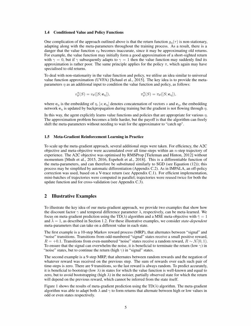
To illustrate the key idea of our meta-gradient approach, we provide two examples that show howthe discount factor γ and temporal difference parameter λ, respectively, can be meta-learned. Wefocus on meta-gradient prediction using the TD(λ) algorithm and a MSE meta-objective with γ̄ = 1and λ̄ = 1, as described in Section 1.2. For these illustrative examples, we consider state-dependentmeta-parameters that can take on a different value in each state.

The first example is a 10-step Markov reward process (MRP), that alternates between “signal” and“noise” transitions. Transitions from odd-numbered “signal” states receive a small positive reward,R = +0.1. Transitions from even-numbered “noise” states receive a random reward, R ∼ N (0, 1).To ensure that the signal can overwhelm the noise, it is beneficial to terminate the return (low γ) in“noise” states, but to continue the return (high γ) in “signal” states.

The second example is a 9-step MRP, that alternates between random rewards and the negation ofwhatever reward was received on the previous step. The sum of rewards over each such pair oftime-steps is zero. There are 9 transitions, so the last reward is always random. To predict accurately,it is beneficial to bootstrap (low λ) in states for which the value function is well-known and equal tozero, but to avoid bootstrapping (high λ) in the noisier, partially observed state for which the returnwill depend on the previous reward, which cannot be inferred from the state itself.

Figure 1 shows the results of meta-gradient prediction using the TD(λ) algorithm. The meta-gradientalgorithm was able to adapt both λ and γ to form returns that alternate between high or low values inodd or even states respectively.

5

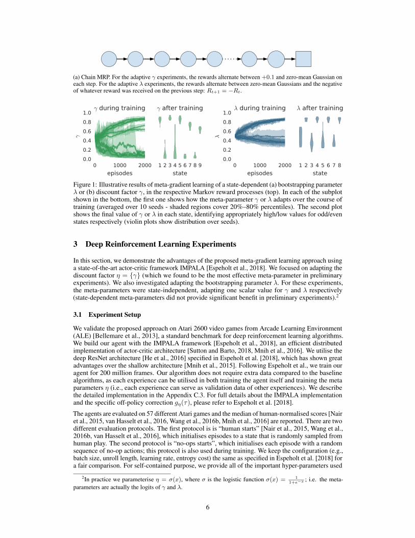
(a) Chain MRP. For the adaptive γ experiments, the rewards alternate between +0.1 and zero-mean Gaussian oneach step. For the adaptive λ experiments, the rewards alternate between zero-mean Gaussians and the negativeof whatever reward was received on the previous step: Rt+1 = −Rt.

0 1000 2000

episodes

0.0

0.2

0.4

0.6

0.8

1.0

γ

γ during training

1 2 3 4 5 6 7 8 9

state

γ after training

0 1000 2000

episodes

0.0

0.2

0.4

0.6

0.8

1.0

λ

λ during training

1 2 3 4 5 6 7 8

state

λ after training

Figure 1: Illustrative results of meta-gradient learning of a state-dependent (a) bootstrapping parameterλ or (b) discount factor γ, in the respective Markov reward processes (top). In each of the subplotshown in the bottom, the first one shows how the meta-parameter γ or λ adapts over the course oftraining (averaged over 10 seeds - shaded regions cover 20%–80% percentiles). The second plotshows the final value of γ or λ in each state, identifying appropriately high/low values for odd/evenstates respectively (violin plots show distribution over seeds).

3 Deep Reinforcement Learning Experiments

In this section, we demonstrate the advantages of the proposed meta-gradient learning approach usinga state-of-the-art actor-critic framework IMPALA [Espeholt et al., 2018]. We focused on adapting thediscount factor η = {γ} (which we found to be the most effective meta-parameter in preliminaryexperiments). We also investigated adapting the bootstrapping parameter λ. For these experiments,the meta-parameters were state-independent, adapting one scalar value for γ and λ respectively(state-dependent meta-parameters did not provide significant benefit in preliminary experiments).2

3.1 Experiment Setup

We validate the proposed approach on Atari 2600 video games from Arcade Learning Environment(ALE) [Bellemare et al., 2013], a standard benchmark for deep reinforcement learning algorithms.We build our agent with the IMPALA framework [Espeholt et al., 2018], an efficient distributedimplementation of actor-critic architecture [Sutton and Barto, 2018, Mnih et al., 2016]. We utilise thedeep ResNet architecture [He et al., 2016] specified in Espeholt et al. [2018], which has shown greatadvantages over the shallow architecture [Mnih et al., 2015]. Following Espeholt et al., we train ouragent for 200 million frames. Our algorithm does not require extra data compared to the baselinealgorithms, as each experience can be utilised in both training the agent itself and training the metaparameters η (i.e., each experience can serve as validation data of other experiences). We describethe detailed implementation in the Appendix C.3. For full details about the IMPALA implementationand the specific off-policy correction gη(τ), please refer to Espeholt et al. [2018].

The agents are evaluated on 57 different Atari games and the median of human-normalised scores [Nairet al., 2015, van Hasselt et al., 2016, Wang et al., 2016b, Mnih et al., 2016] are reported. There are twodifferent evaluation protocols. The first protocol is is “human starts” [Nair et al., 2015, Wang et al.,2016b, van Hasselt et al., 2016], which initialises episodes to a state that is randomly sampled fromhuman play. The second protocol is “no-ops starts”, which initialises each episode with a randomsequence of no-op actions; this protocol is also used during training. We keep the configuration (e.g.,batch size, unroll length, learning rate, entropy cost) the same as specified in Espeholt et al. [2018] fora fair comparison. For self-contained purpose, we provide all of the important hyper-parameters used

2In practice we parameterise η = σ(x), where σ is the logistic function σ(x) = 11+e−x ; i.e. the meta-

parameters are actually the logits of γ and λ.

6

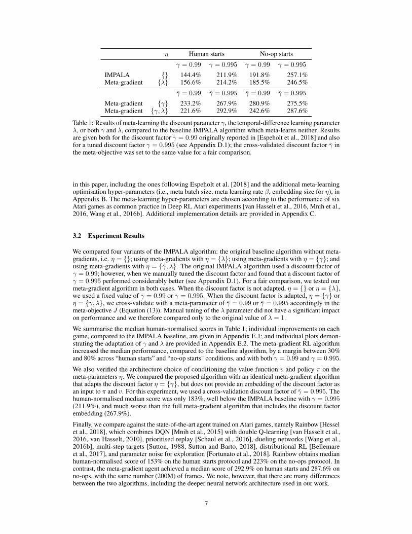
η Human starts No-op starts

γ = 0.99 γ = 0.995 γ = 0.99 γ = 0.995

IMPALA {} 144.4% 211.9% 191.8% 257.1%Meta-gradient {λ} 156.6% 214.2% 185.5% 246.5%

γ̄ = 0.99 γ̄ = 0.995 γ̄ = 0.99 γ̄ = 0.995

Meta-gradient {γ} 233.2% 267.9% 280.9% 275.5%Meta-gradient {γ, λ} 221.6% 292.9% 242.6% 287.6%

Table 1: Results of meta-learning the discount parameter γ, the temporal-difference learning parameterλ, or both γ and λ, compared to the baseline IMPALA algorithm which meta-learns neither. Resultsare given both for the discount factor γ = 0.99 originally reported in [Espeholt et al., 2018] and alsofor a tuned discount factor γ = 0.995 (see Appendix D.1); the cross-validated discount factor γ̄ inthe meta-objective was set to the same value for a fair comparison.

in this paper, including the ones following Espeholt et al. [2018] and the additional meta-learningoptimisation hyper-parameters (i.e., meta batch size, meta learning rate β, embedding size for η), inAppendix B. The meta-learning hyper-parameters are chosen according to the performance of sixAtari games as common practice in Deep RL Atari experiments [van Hasselt et al., 2016, Mnih et al.,2016, Wang et al., 2016b]. Additional implementation details are provided in Appendix C.

3.2 Experiment Results

We compared four variants of the IMPALA algorithm: the original baseline algorithm without meta-gradients, i.e. η = {}; using meta-gradients with η = {λ}; using meta-gradients with η = {γ}; andusing meta-gradients with η = {γ, λ}. The original IMPALA algorithm used a discount factor ofγ = 0.99; however, when we manually tuned the discount factor and found that a discount factor ofγ = 0.995 performed considerably better (see Appendix D.1). For a fair comparison, we tested ourmeta-gradient algorithm in both cases. When the discount factor is not adapted, η = {} or η = {λ},we used a fixed value of γ = 0.99 or γ = 0.995. When the discount factor is adapted, η = {γ} orη = {γ, λ}, we cross-validate with a meta-parameter of γ̄ = 0.99 or γ̄ = 0.995 accordingly in themeta-objective J̄ (Equation (13)). Manual tuning of the λ parameter did not have a significant impacton performance and we therefore compared only to the original value of λ = 1.

We summarise the median human-normalised scores in Table 1; individual improvements on eachgame, compared to the IMPALA baseline, are given in Appendix E.1; and individual plots demon-strating the adaptation of γ and λ are provided in Appendix E.2. The meta-gradient RL algorithmincreased the median performance, compared to the baseline algorithm, by a margin between 30%and 80% across “human starts” and “no-op starts" conditions, and with both γ = 0.99 and γ = 0.995.

We also verified the architecture choice of conditioning the value function v and policy π on themeta-parameters η. We compared the proposed algorithm with an identical meta-gradient algorithmthat adapts the discount factor η = {γ}, but does not provide an embedding of the discount factor asan input to π and v. For this experiment, we used a cross-validation discount factor of γ̄ = 0.995. Thehuman-normalised median score was only 183%, well below the IMPALA baseline with γ = 0.995(211.9%), and much worse than the full meta-gradient algorithm that includes the discount factorembedding (267.9%).

Finally, we compare against the state-of-the-art agent trained on Atari games, namely Rainbow [Hesselet al., 2018], which combines DQN [Mnih et al., 2015] with double Q-learning [van Hasselt et al.,2016, van Hasselt, 2010], prioritised replay [Schaul et al., 2016], dueling networks [Wang et al.,2016b], multi-step targets [Sutton, 1988, Sutton and Barto, 2018], distributional RL [Bellemareet al., 2017], and parameter noise for exploration [Fortunato et al., 2018]. Rainbow obtains medianhuman-normalised score of 153% on the human starts protocol and 223% on the no-ops protocol. Incontrast, the meta-gradient agent achieved a median score of 292.9% on human starts and 287.6% onno-ops, with the same number (200M) of frames. We note, however, that there are many differencesbetween the two algorithms, including the deeper neural network architecture used in our work.

7

4 Related Work

Among the earliest studies on meta learning (or learning to learn [Thrun and Pratt, 1998]), Schmid-huber [1987] applied genetic programming to itself to evolve better genetic programming algo-rithms. Hochreiter et al. [2001] used recurrent neural networks like Long Short-Term Memory(LSTM) [Hochreiter and Schmidhuber, 1997] as meta-learners. A recent direction of research hasbeen to meta-learn an optimiser using a recurrent parameterisation [Andrychowicz et al., 2016,Wichrowska et al., 2017]. Duan et al. [2016] and Wang et al. [2016a] proposed to learn a recurrentmeta-policy that itself learns to solve the reinforcement learning problem, so that the recurrentpolicy can generalise into new tasks faster than learning the policy from scratch. Model-AgnosticMeta-Learning (MAML) [Finn et al., 2017a, Finn and Levine, 2018, Finn et al., 2017b, Grant et al.,2018, Al-Shedivat et al., 2018] learns a good initialisation of the model that can adapt quickly toother tasks within a few gradient update steps. These works focus on a multi-task setting in whichmeta-learning takes place on a distribution of training tasks, to facilitate fast adaptation on an unseentest task. In contrast, our work emphasises the (arguably) more fundamental problem of meta-learningwithin a single task. In other words we return to the standard formulation of RL as maximisingrewards during a single lifetime of interactions with an environment.

Contemporaneously with our own work, Zheng et al. [2018] also propose a similar algorithm to learnmeta-parameters of the return: in their case an auxiliary reward function that is added to the externalrewards. They do not condition their value function or policy, and reuse the same samples for boththe update function and the cross-validation step – which may be problematic in stochastic domainswhen the noise these updates becomes highly correlated.

There are many works focusing on adapting learning rate through gradient-based methods [Sutton,1992, Schraudolph, 1999, Maclaurin et al., 2015, Pedregosa, 2016, Franceschi et al., 2017], Bayesianoptimisation methods [Snoek et al., 2012], or evolution based hyper-parameter tuning [Jaderberget al., 2017a, Elfwing et al., 2017]. In particular, Sutton [1992], introduced the idea of online cross-validation; however, this method was limited in scope to adapting the learning rate for linear updatesin supervised learning (later extended to non-linear updates by Schraudolph [1999]); whereas wefocus on the fundamental problem of reinforcement learning, i.e., adapting the return function tomaximise the proxy returns we can achieve from the environment.

There has also been significant prior work on automatically adapting the bootstrapping parameterλ. Singh and Dayan [1998] empirically analyse the effect of λ in terms of bias, variance and MSE.Kearns and Singh [2000] derive upper bounds on the error of temporal-difference algorithms, and usethese bounds to derive schedules for λ. Downey and Sanner [2010] introduced a Bayesian modelaveraging approach to scheduling λ. Konidaris et al. [2011] derive a maximum-likelihood estimator,TD(γ), that weights the n-step returns according to the discount factor, leading to a parameter-freealgorithm for temporal-difference learning with linear function approximation. White and White[2016] introduce an algorithm that explicitly estimates the bias and variance, and greedily adapts λ tolocally minimise the MSE of the λ-return. Unlike our meta-gradient approach, these prior approachesexploit i.i.d. assumptions on the trajectory of experience that are not realistic in many applications.

5 Conclusion

In this work, we discussed how to learn the meta-parameters of a return function. Our meta-learningalgorithm runs online, while interacting with a single environment, and successfully adapts the returnto produce better performance. We demonstrated, by adjusting the meta-parameters of a state-of-the-art deep learning algorithm, that we could achieve much higher performance than previouslyobserved on 57 Atari 2600 games from the Arcade Learning Environment.

Our proposed method is more general, and can be applied not just to the discount factor or bootstrap-ping parameter, but also to other components of the return, and even more generally to the learningupdate itself. Hyper-parameter tuning has been a thorn in the side of reinforcement learning researchfor several decades. Our hope is that this approach will allow agents to automatically tune their ownhyper-parameters, by exposing them as meta-parameters of the learning update. This may also resultin better performance because the parameters can change over time and adapt to novel environments.

8

Acknowledgements

The authors would like to thank Matteo Hessel, Lasse Espeholt, Hubert Soyer, Dan Horgan, AedanPope and Tim Harley for their kind engineering support; and Joseph Modayil, Andre Barreto for theirsuggestions and comments on an early version of the paper. The authors would also like to thankanonymous reviewers for their constructive suggestions on improving the paper.

9

ReferencesM. Abadi, P. Barham, J. Chen, Z. Chen, A. Davis, J. Dean, M. Devin, S. Ghemawat, G. Irving,

M. Isard, et al. TensorFlow: A system for large-scale machine learning. In OSDI, volume 16,pages 265–283, 2016.

M. Al-Shedivat, T. Bansal, Y. Burda, I. Sutskever, I. Mordatch, and P. Abbeel. Continuous adaptationvia meta-learning in nonstationary and competitive environments. In ICLR, 2018.

M. Andrychowicz, M. Denil, S. Gomez, M. W. Hoffman, D. Pfau, T. Schaul, and N. de Freitas.Learning to learn by gradient descent by gradient descent. In NIPS, pages 3981–3989, 2016.

M. G. Bellemare, Y. Naddaf, J. Veness, and M. Bowling. The arcade learning environment: Anevaluation platform for general agents. J. Artif. Intell. Res.(JAIR), 47:253–279, 2013.

M. G. Bellemare, W. Dabney, and R. Munos. A distributional perspective on reinforcement learning.In ICML, 2017.

D. P. Bertsekas and J. N. Tsitsiklis. Neuro-Dynamic Programming. Athena Scientific, 1996.

C. Downey and S. Sanner. Temporal difference bayesian model averaging: A bayesian perspectiveon adapting lambda. In ICML, pages 311–318. Citeseer, 2010.

Y. Duan, J. Schulman, X. Chen, P. L. Bartlett, I. Sutskever, and P. Abbeel. RL2: Fast reinforcementlearning via slow reinforcement learning. arXiv preprint arXiv:1611.02779, 2016.

S. Elfwing, E. Uchibe, and K. Doya. Online meta-learning by parallel algorithm competition. CoRR,abs/1702.07490, 2017.

L. Espeholt, H. Soyer, R. Munos, K. Simonyan, V. Mnih, T. Ward, Y. Doron, V. Firoiu, T. Harley,I. Dunning, et al. IMPALA: Scalable distributed Deep-RL with importance weighted actor-learnerarchitectures. ICML, 2018.

C. Finn and S. Levine. Meta-learning and universality: Deep representations and gradient descentcan approximate any learning algorithm. ICLR, 2018.

C. Finn, P. Abbeel, and S. Levine. Model-agnostic meta-learning for fast adaptation of deep networks.In ICML, 2017a.

C. Finn, T. Yu, T. Zhang, P. Abbeel, and S. Levine. One-shot visual imitation learning via meta-learning. In CoRL, 2017b.

M. Fortunato, M. G. Azar, B. Piot, J. Menick, I. Osband, A. Graves, V. Mnih, R. Munos, D. Hassabis,O. Pietquin, et al. Noisy networks for exploration. In ICLR, 2018.

L. Franceschi, M. Donini, P. Frasconi, and M. Pontil. Forward and reverse gradient-based hyperpa-rameter optimization. In ICML, 2017.

E. Grant, C. Finn, S. Levine, T. Darrell, and T. Griffiths. Recasting gradient-based meta-learning ashierarchical Bayes. ICLR, 2018.

A. Harutyunyan, M. G. Bellemare, T. Stepleton, and R. Munos. Q(λ) with off-policy corrections. InALT, pages 305–320. Springer, 2016.

K. He, X. Zhang, S. Ren, and J. Sun. Deep residual learning for image recognition. In CVPR, pages770–778, 2016.

M. Hessel, J. Modayil, H. Van Hasselt, T. Schaul, G. Ostrovski, W. Dabney, D. Horgan, B. Piot,M. Azar, and D. Silver. Rainbow: Combining improvements in deep reinforcement learning. InAAAI, 2018.

S. Hochreiter and J. Schmidhuber. Long short-term memory. Neural computation, 9(8):1735–1780,1997.

S. Hochreiter, A. S. Younger, and P. R. Conwell. Learning to learn using gradient descent. In ICANN,pages 87–94. Springer, 2001.

10

M. Jaderberg, V. Dalibard, S. Osindero, W. M. Czarnecki, J. Donahue, A. Razavi, O. Vinyals,T. Green, I. Dunning, K. Simonyan, et al. Population based training of neural networks. arXivpreprint arXiv:1711.09846, 2017a.

M. Jaderberg, V. Mnih, W. M. Czarnecki, T. Schaul, J. Z. Leibo, D. Silver, and K. Kavukcuoglu.Reinforcement learning with unsupervised auxiliary tasks. In ICLR, 2017b.

M. J. Kearns and S. P. Singh. Bias-variance error bounds for temporal difference updates. In COLT,pages 142–147, 2000.

D. P. Kingma and J. Ba. ADAM: A method for stochastic optimization. ICLR, 2015.

G. Konidaris, S. Niekum, and P. S. Thomas. TDγ : Re-evaluating complex backups in temporaldifference learning. In NIPS, pages 2402–2410, 2011.

D. Maclaurin, D. Duvenaud, and R. Adams. Gradient-based hyperparameter optimization throughreversible learning. In ICML, pages 2113–2122, 2015.

A. Mahmood. Incremental Off-policy Reinforcement Learning Algorithms. PhD thesis, University ofAlberta, 2017.

V. Mnih, K. Kavukcuoglu, D. Silver, A. Graves, I. Antonoglou, D. Wierstra, and M. Riedmiller.Playing atari with deep reinforcement learning. NIPS workshop, 2013.

V. Mnih, K. Kavukcuoglu, D. Silver, A. A. Rusu, J. Veness, M. G. Bellemare, A. Graves, M. Ried-miller, A. K. Fidjeland, G. Ostrovski, et al. Human-level control through deep reinforcementlearning. Nature, 518(7540):529, 2015.

V. Mnih, A. P. Badia, M. Mirza, A. Graves, T. Lillicrap, T. Harley, D. Silver, and K. Kavukcuoglu.Asynchronous methods for deep reinforcement learning. In ICML, pages 1928–1937, 2016.

R. Munos, T. Stepleton, A. Harutyunyan, and M. Bellemare. Safe and efficient off-policy reinforce-ment learning. In NIPS, pages 1054–1062, 2016.

A. Nair, P. Srinivasan, S. Blackwell, C. Alcicek, R. Fearon, A. De Maria, V. Panneershelvam,M. Suleyman, C. Beattie, S. Petersen, et al. Massively parallel methods for deep reinforcementlearning. arXiv preprint arXiv:1507.04296, 2015.

F. Pedregosa. Hyperparameter optimization with approximate gradient. In ICML, pages 737–746,2016.

D. Precup, R. S. Sutton, and S. P. Singh. Eligibility traces for off-policy policy evaluation. In ICML,pages 759–766, 2000.

D. V. Prokhorov and D. C. Wunsch. Adaptive critic designs. TNN, 8(5):997–1007, 1997.

J. Randløv and P. Alstrøm. Learning to drive a bicycle using reinforcement learning and shaping. InICML, volume 98, pages 463–471, 1998.

G. A. Rummery and M. Niranjan. On-line Q-learning using connectionist sytems. Technical ReportCUED/F-INFENG-TR 166, Cambridge University, UK, 1994.

T. Schaul, D. Horgan, K. Gregor, and D. Silver. Universal value function approximators. In ICML,pages 1312–1320, 2015.

T. Schaul, J. Quan, I. Antonoglou, and D. Silver. Prioritized experience replay. In ICLR, 2016.

J. Schmidhuber. Evolutionary principles in self-referential learning, or on learning how to learn: themeta-meta-... hook. PhD thesis, Technische Universität München, 1987.

N. N. Schraudolph. Local gain adaptation in stochastic gradient descent. In ICANN. IET, 1999.

S. Singh and P. Dayan. Analytical mean squared error curves for temporal difference learning.Machine Learning, 32(1):5–40, 1998.

11

S. P. Singh, A. G. Barto, and N. Chentanez. Intrinsically motivated reinforcement learning. In NIPS,pages 1281–1288, 2005.

J. Snoek, H. Larochelle, and R. P. Adams. Practical Bayesian optimization of machine learningalgorithms. In NIPS, pages 2951–2959, 2012.

R. S. Sutton. Learning to predict by the methods of temporal differences. Machine learning, 3(1):9–44, 1988.

R. S. Sutton. Adapting bias by gradient descent: An incremental version of delta-bar-delta. In AAAI,pages 171–176, 1992.

R. S. Sutton and A. G. Barto. Reinforcement learning: An introduction. MIT press Cambridge, 2018.

R. S. Sutton, A. R. Mahmood, D. Precup, and H. van Hasselt. A new Q(λ) with interim forward viewand Monte Carlo equivalence. In ICML, pages 568–576, 2014.

R. S. Sutton, A. R. Mahmood, and M. White. An emphatic approach to the problem of off-policytemporal-difference learning. JMLR, 17(1):2603–2631, 2016.

S. Thrun and L. Pratt. Learning to learn. Springer Science & Business Media, 1998.

T. Tieleman and G. Hinton. Lecture 6.5-RMSProp: Divide the gradient by a running average of itsrecent magnitude. COURSERA: Neural networks for machine learning, 4(2):26–31, 2012.

H. van Hasselt. Double Q-learning. In NIPS, pages 2613–2621, 2010.

H. van Hasselt, A. Guez, and D. Silver. Deep reinforcement learning with double Q-learning. InAAAI, volume 16, pages 2094–2100, 2016.

H. H. van Seijen, H. P. van Hasselt, S. Whiteson, and M. A. Wiering. A theoretical and empiricalanalysis of Expected Sarsa. In ADPRL, pages 177–184, 2009.

J. X. Wang, Z. Kurth-Nelson, D. Tirumala, H. Soyer, J. Z. Leibo, R. Munos, C. Blundell, D. Kumaran,and M. Botvinick. Learning to reinforcement learn. arXiv preprint arXiv:1611.05763, 2016a.

Z. Wang, T. Schaul, M. Hessel, H. Van Hasselt, M. Lanctot, and N. De Freitas. Dueling networkarchitectures for deep reinforcement learning. ICML, 2016b.

M. White and A. White. A greedy approach to adapting the trace parameter for temporal differencelearning. In AAMAS, pages 557–565, 2016.

O. Wichrowska, N. Maheswaranathan, M. W. Hoffman, S. G. Colmenarejo, M. Denil, N. de Freitas,and J. Sohl-Dickstein. Learned optimizers that scale and generalize. In ICML, 2017.

R. J. Williams. Simple statistical gradient-following algorithms for connectionist reinforcementlearning. Machine Learning, 8(3-4):229–256, May 1992.

R. J. Williams and D. Zipser. A learning algorithm for continually running fully recurrent neuralnetworks. Neural computation, 1(2):270–280, 1989.

Z. Zheng, J. Oh, and S. Singh. On learning intrinsic rewards for policy gradient methods. In NeurIPS,2018.

12