Deep Reinforcement Learning with Double Q-learning

Hado van Hasselt and Arthur Guez and David SilverGoogle DeepMind

Abstract

The popular Q-learning algorithm is known to overestimateaction values under certain conditions. It was not previouslyknown whether, in practice, such overestimations are com-mon, whether they harm performance, and whether they cangenerally be prevented. In this paper, we answer all thesequestions affirmatively. In particular, we first show that therecent DQN algorithm, which combines Q-learning with adeep neural network, suffers from substantial overestimationsin some games in the Atari 2600 domain. We then show thatthe idea behind the Double Q-learning algorithm, which wasintroduced in a tabular setting, can be generalized to workwith large-scale function approximation. We propose a spe-cific adaptation to the DQN algorithm and show that the re-sulting algorithm not only reduces the observed overestima-tions, as hypothesized, but that this also leads to much betterperformance on several games.

The goal of reinforcement learning (Sutton and Barto, 1998)is to learn good policies for sequential decision problems,by optimizing a cumulative future reward signal. Q-learning(Watkins, 1989) is one of the most popular reinforcementlearning algorithms, but it is known to sometimes learn un-realistically high action values because it includes a maxi-mization step over estimated action values, which tends toprefer overestimated to underestimated values.

In previous work, overestimations have been attributedto insufficiently flexible function approximation (Thrun andSchwartz, 1993) and noise (van Hasselt, 2010, 2011). Inthis paper, we unify these views and show overestimationscan occur when the action values are inaccurate, irrespectiveof the source of approximation error. Of course, imprecisevalue estimates are the norm during learning, which indi-cates that overestimations may be much more common thanpreviously appreciated.

It is an open question whether, if the overestimationsdo occur, this negatively affects performance in practice.Overoptimistic value estimates are not necessarily a prob-lem in and of themselves. If all values would be uniformlyhigher then the relative action preferences are preserved andwe would not expect the resulting policy to be any worse.Furthermore, it is known that sometimes it is good to be op-timistic: optimism in the face of uncertainty is a well-known

Copyright c© 2016, Association for the Advancement of ArtificialIntelligence (www.aaai.org). All rights reserved.

exploration technique (Kaelbling et al., 1996). If, however,the overestimations are not uniform and not concentrated atstates about which we wish to learn more, then they mightnegatively affect the quality of the resulting policy. Thrunand Schwartz (1993) give specific examples in which thisleads to suboptimal policies, even asymptotically.

To test whether overestimations occur in practice and atscale, we investigate the performance of the recent DQN al-gorithm (Mnih et al., 2015). DQN combines Q-learning witha flexible deep neural network and was tested on a variedand large set of deterministic Atari 2600 games, reachinghuman-level performance on many games. In some ways,this setting is a best-case scenario for Q-learning, becausethe deep neural network provides flexible function approx-imation with the potential for a low asymptotic approxima-tion error, and the determinism of the environments preventsthe harmful effects of noise. Perhaps surprisingly, we showthat even in this comparatively favorable setting DQN some-times substantially overestimates the values of the actions.

We show that the idea behind the Double Q-learning algo-rithm (van Hasselt, 2010), which was first proposed in a tab-ular setting, can be generalized to work with arbitrary func-tion approximation, including deep neural networks. We usethis to construct a new algorithm we call Double DQN. Wethen show that this algorithm not only yields more accuratevalue estimates, but leads to much higher scores on severalgames. This demonstrates that the overestimations of DQNwere indeed leading to poorer policies and that it is benefi-cial to reduce them. In addition, by improving upon DQNwe obtain state-of-the-art results on the Atari domain.

BackgroundTo solve sequential decision problems we can learn esti-mates for the optimal value of each action, defined as theexpected sum of future rewards when taking that action andfollowing the optimal policy thereafter. Under a given policyπ, the true value of an action a in a state s is

Qπ(s, a) ≡ E [R1 + γR2 + . . . | S0 = s,A0 = a, π] ,

where γ ∈ [0, 1] is a discount factor that trades off the impor-tance of immediate and later rewards. The optimal value isthen Q∗(s, a) = maxπ Qπ(s, a). An optimal policy is eas-ily derived from the optimal values by selecting the highest-valued action in each state.

arX

iv:1

509.

0646

1v3

[cs

.LG

] 8

Dec

201

5

Estimates for the optimal action values can be learnedusing Q-learning (Watkins, 1989), a form of temporal dif-ference learning (Sutton, 1988). Most interesting problemsare too large to learn all action values in all states sepa-rately. Instead, we can learn a parameterized value functionQ(s, a;θt). The standard Q-learning update for the param-eters after taking action At in state St and observing theimmediate reward Rt+1 and resulting state St+1 is then

θt+1 = θt+α(YQt −Q(St, At;θt))∇θt

Q(St, At;θt) . (1)

where α is a scalar step size and the target Y Qt is defined as

Y Qt ≡ Rt+1 + γmax

aQ(St+1, a;θt) . (2)

This update resembles stochastic gradient descent, updatingthe current value Q(St, At;θt) towards a target value Y Q

t .

Deep Q NetworksA deep Q network (DQN) is a multi-layered neural networkthat for a given state s outputs a vector of action valuesQ(s, · ;θ), where θ are the parameters of the network. Foran n-dimensional state space and an action space contain-ing m actions, the neural network is a function from Rn toRm. Two important ingredients of the DQN algorithm asproposed by Mnih et al. (2015) are the use of a target net-work, and the use of experience replay. The target network,with parameters θ−, is the same as the online network ex-cept that its parameters are copied every τ steps from theonline network, so that then θ−t = θt, and kept fixed on allother steps. The target used by DQN is then

Y DQNt ≡ Rt+1 + γmax

aQ(St+1, a;θ

−t ) . (3)

For the experience replay (Lin, 1992), observed transitionsare stored for some time and sampled uniformly from thismemory bank to update the network. Both the target networkand the experience replay dramatically improve the perfor-mance of the algorithm (Mnih et al., 2015).

Double Q-learningThe max operator in standard Q-learning and DQN, in (2)and (3), uses the same values both to select and to evalu-ate an action. This makes it more likely to select overesti-mated values, resulting in overoptimistic value estimates. Toprevent this, we can decouple the selection from the evalua-tion. This is the idea behind Double Q-learning (van Hasselt,2010).

In the original Double Q-learning algorithm, two valuefunctions are learned by assigning each experience ran-domly to update one of the two value functions, such thatthere are two sets of weights, θ and θ′. For each update, oneset of weights is used to determine the greedy policy and theother to determine its value. For a clear comparison, we canfirst untangle the selection and evaluation in Q-learning andrewrite its target (2) as

Y Qt = Rt+1 + γQ(St+1, argmax

aQ(St+1, a;θt);θt) .

The Double Q-learning error can then be written as

Y DoubleQt ≡ Rt+1 + γQ(St+1, argmax

aQ(St+1, a;θt);θ

′t) .

(4)Notice that the selection of the action, in the argmax, isstill due to the online weights θt. This means that, as in Q-learning, we are still estimating the value of the greedy pol-icy according to the current values, as defined by θt. How-ever, we use the second set of weights θ′t to fairly evaluatethe value of this policy. This second set of weights can beupdated symmetrically by switching the roles of θ and θ′.

Overoptimism due to estimation errorsQ-learning’s overestimations were first investigated byThrun and Schwartz (1993), who showed that if the actionvalues contain random errors uniformly distributed in an in-terval [−ε, ε] then each target is overestimated up to γεm−1m+1 ,where m is the number of actions. In addition, Thrun andSchwartz give a concrete example in which these overes-timations even asymptotically lead to sub-optimal policies,and show the overestimations manifest themselves in a smalltoy problem when using function approximation. Later vanHasselt (2010) argued that noise in the environment can leadto overestimations even when using tabular representation,and proposed Double Q-learning as a solution.

In this section we demonstrate more generally that esti-mation errors of any kind can induce an upward bias, re-gardless of whether these errors are due to environmentalnoise, function approximation, non-stationarity, or any othersource. This is important, because in practice any methodwill incur some inaccuracies during learning, simply due tothe fact that the true values are initially unknown.

The result by Thrun and Schwartz (1993) cited abovegives an upper bound to the overestimation for a specificsetup, but it is also possible, and potentially more interest-ing, to derive a lower bound.Theorem 1. Consider a state s in which all the true optimalaction values are equal atQ∗(s, a) = V∗(s) for some V∗(s).LetQt be arbitrary value estimates that are on the whole un-biased in the sense that

∑a(Qt(s, a)−V∗(s)) = 0, but that

are not all correct, such that 1m

∑a(Qt(s, a)−V∗(s))2 = C

for some C > 0, where m ≥ 2 is the number of actions in s.

Under these conditions, maxaQt(s, a) ≥ V∗(s) +√

Cm−1 .

This lower bound is tight. Under the same conditions, thelower bound on the absolute error of the Double Q-learningestimate is zero. (Proof in appendix.)

Note that we did not need to assume that estimation errorsfor different actions are independent. This theorem showsthat even if the value estimates are on average correct, esti-mation errors of any source can drive the estimates up andaway from the true optimal values.

The lower bound in Theorem 1 decreases with the num-ber of actions. This is an artifact of considering the lowerbound, which requires very specific values to be attained.More typically, the overoptimism increases with the num-ber of actions as shown in Figure 1. Q-learning’s overesti-mations there indeed increase with the number of actions,

2 4 8 16 32 64 1282565121024

number of actions

0.0

0.5

1.0

1.5er

ror

maxaQ(s, a)− V∗(s)Q′(s, argmaxaQ(s, a))− V∗(s)

Figure 1: The orange bars show the bias in a single Q-learning update when the action values are Q(s, a) =V∗(s) + εa and the errors {εa}ma=1 are independent standardnormal random variables. The second set of action valuesQ′, used for the blue bars, was generated identically and in-dependently. All bars are the average of 100 repetitions.

while Double Q-learning is unbiased. As another example,if for all actions Q∗(s, a) = V∗(s) and the estimation errorsQt(s, a) − V∗(s) are uniformly random in [−1, 1], then theoveroptimism is m−1

m+1 . (Proof in appendix.)We now turn to function approximation and consider a

real-valued continuous state space with 10 discrete actionsin each state. For simplicity, the true optimal action valuesin this example depend only on state so that in each stateall actions have the same true value. These true values areshown in the left column of plots in Figure 2 (purple lines)and are defined as either Q∗(s, a) = sin(s) (top row) orQ∗(s, a) = 2 exp(−s2) (middle and bottom rows). The leftplots also show an approximation for a single action (greenlines) as a function of state as well as the samples the es-timate is based on (green dots). The estimate is a d-degreepolynomial that is fit to the true values at sampled states,where d = 6 (top and middle rows) or d = 9 (bottomrow). The samples match the true function exactly: there isno noise and we assume we have ground truth for the actionvalue on these sampled states. The approximation is inex-act even on the sampled states for the top two rows becausethe function approximation is insufficiently flexible. In thebottom row, the function is flexible enough to fit the greendots, but this reduces the accuracy in unsampled states. No-tice that the sampled states are spaced further apart near theleft side of the left plots, resulting in larger estimation errors.In many ways this is a typical learning setting, where at eachpoint in time we only have limited data.

The middle column of plots in Figure 2 shows estimatedaction value functions for all 10 actions (green lines), asfunctions of state, along with the maximum action value ineach state (black dashed line). Although the true value func-tion is the same for all actions, the approximations differbecause we have supplied different sets of sampled states.1The maximum is often higher than the ground truth shownin purple on the left. This is confirmed in the right plots,which shows the difference between the black and purplecurves in orange. The orange line is almost always positive,

1Each action-value function is fit with a different subset of in-teger states. States −6 and 6 are always included to avoid extrap-olations, and for each action two adjacent integers are missing: foraction a1 states −5 and −4 are not sampled, for a2 states −4 and−3 are not sampled, and so on. This causes the estimated values todiffer.

indicating an upward bias. The right plots also show the es-timates from Double Q-learning in blue2, which are on aver-age much closer to zero. This demonstrates that Double Q-learning indeed can successfully reduce the overoptimism ofQ-learning.

The different rows in Figure 2 show variations of the sameexperiment. The difference between the top and middle rowsis the true value function, demonstrating that overestima-tions are not an artifact of a specific true value function.The difference between the middle and bottom rows is theflexibility of the function approximation. In the left-middleplot, the estimates are even incorrect for some of the sam-pled states because the function is insufficiently flexible.The function in the bottom-left plot is more flexible but thiscauses higher estimation errors for unseen states, resultingin higher overestimations. This is important because flexi-ble parametric function approximators are often employedin reinforcement learning (see, e.g., Tesauro 1995; Sallansand Hinton 2004; Riedmiller 2005; Mnih et al. 2015).

In contrast to van Hasselt (2010) we did not use a sta-tistical argument to find overestimations, the process to ob-tain Figure 2 is fully deterministic. In contrast to Thrun andSchwartz (1993), we did not rely on inflexible function ap-proximation with irreducible asymptotic errors; the bottomrow shows that a function that is flexible enough to cover allsamples leads to high overestimations. This indicates thatthe overestimations can occur quite generally.

In the examples above, overestimations occur even whenassuming we have samples of the true action value at cer-tain states. The value estimates can further deteriorate if webootstrap off of action values that are already overoptimistic,since this causes overestimations to propagate throughoutour estimates. Although uniformly overestimating valuesmight not hurt the resulting policy, in practice overestima-tion errors will differ for different states and actions. Over-estimation combined with bootstrapping then has the perni-cious effect of propagating the wrong relative informationabout which states are more valuable than others, directlyaffecting the quality of the learned policies.

The overestimations should not be confused with opti-mism in the face of uncertainty (Sutton, 1990; Agrawal,1995; Kaelbling et al., 1996; Auer et al., 2002; Brafman andTennenholtz, 2003; Szita and Lorincz, 2008; Strehl et al.,2009), where an exploration bonus is given to states oractions with uncertain values. Conversely, the overestima-tions discussed here occur only after updating, resulting inoveroptimism in the face of apparent certainty. This was al-ready observed by Thrun and Schwartz (1993), who notedthat, in contrast to optimism in the face of uncertainty, theseoverestimations actually can impede learning an optimalpolicy. We will see this negative effect on policy quality con-firmed later in the experiments as well: when we reduce theoverestimations using Double Q-learning, the policies im-prove.

2We arbitrarily used the samples of action ai+5 (for i ≤ 5)or ai−5 (for i > 5) as the second set of samples for the doubleestimator of action ai.

−2

0

2

Qt(s, a)

Q∗(s, a)

True value and an estimate

−2

0

2maxaQt(s, a)

All estimates and max

−1

0

1maxaQt(s, a)−maxaQ∗(s, a)

Double-Q estimate

+0.61

−0.02

Average errorBias as function of state

0

2

Qt(s, a)

Q∗(s, a)

0

2 maxaQt(s, a)

−1

0

1maxaQt(s, a)−maxaQ∗(s, a)

Double-Q estimate

+0.47

+0.02

−6 −4 −2 0 2 4 6

state

0

2

4Qt(s, a)

Q∗(s, a)

−6 −4 −2 0 2 4 6

state

0

2

4maxaQt(s, a)

−6 −4 −2 0 2 4 6

state

0

2

4 maxaQt(s, a)−maxaQ∗(s, a)

Double-Q estimate

+3.35

−0.02

Figure 2: Illustration of overestimations during learning. In each state (x-axis), there are 10 actions. The left column shows the true valuesV∗(s) (purple line). All true action values are defined by Q∗(s, a) = V∗(s). The green line shows estimated values Q(s, a) for one actionas a function of state, fitted to the true value at several sampled states (green dots). The middle column plots show all the estimated values(green), and the maximum of these values (dashed black). The maximum is higher than the true value (purple, left plot) almost everywhere.The right column plots shows the difference in orange. The blue line in the right plots is the estimate used by Double Q-learning with asecond set of samples for each state. The blue line is much closer to zero, indicating less bias. The three rows correspond to different truefunctions (left, purple) or capacities of the fitted function (left, green). (Details in the text)

Double DQNThe idea of Double Q-learning is to reduce overestimationsby decomposing the max operation in the target into actionselection and action evaluation. Although not fully decou-pled, the target network in the DQN architecture providesa natural candidate for the second value function, withouthaving to introduce additional networks. We therefore pro-pose to evaluate the greedy policy according to the onlinenetwork, but using the target network to estimate its value.In reference to both Double Q-learning and DQN, we referto the resulting algorithm as Double DQN. Its update is thesame as for DQN, but replacing the target Y DQN

t with

Y DoubleDQNt ≡ Rt+1+γQ(St+1, argmax

aQ(St+1, a;θt),θ

−t ) .

In comparison to Double Q-learning (4), the weights of thesecond network θ′t are replaced with the weights of the tar-get network θ−t for the evaluation of the current greedy pol-icy. The update to the target network stays unchanged fromDQN, and remains a periodic copy of the online network.

This version of Double DQN is perhaps the minimal pos-sible change to DQN towards Double Q-learning. The goalis to get most of the benefit of Double Q-learning, whilekeeping the rest of the DQN algorithm intact for a fair com-parison, and with minimal computational overhead.

Empirical resultsIn this section, we analyze the overestimations of DQN andshow that Double DQN improves over DQN both in terms ofvalue accuracy and in terms of policy quality. To further testthe robustness of the approach we additionally evaluate thealgorithms with random starts generated from expert humantrajectories, as proposed by Nair et al. (2015).

Our testbed consists of Atari 2600 games, using the Ar-cade Learning Environment (Bellemare et al., 2013). The

goal is for a single algorithm, with a fixed set of hyperpa-rameters, to learn to play each of the games separately frominteraction given only the screen pixels as input. This is a de-manding testbed: not only are the inputs high-dimensional,the game visuals and game mechanics vary substantially be-tween games. Good solutions must therefore rely heavilyon the learning algorithm — it is not practically feasible tooverfit the domain by relying only on tuning.

We closely follow the experimental setting and net-work architecture outlined by Mnih et al. (2015). Briefly,the network architecture is a convolutional neural network(Fukushima, 1988; LeCun et al., 1998) with 3 convolutionlayers and a fully-connected hidden layer (approximately1.5M parameters in total). The network takes the last fourframes as input and outputs the action value of each action.On each game, the network is trained on a single GPU for200M frames, or approximately 1 week.

Results on overoptimism

Figure 3 shows examples of DQN’s overestimations in sixAtari games. DQN and Double DQN were both trained un-der the exact conditions described by Mnih et al. (2015).DQN is consistently and sometimes vastly overoptimisticabout the value of the current greedy policy, as can be seenby comparing the orange learning curves in the top row ofplots to the straight orange lines, which represent the ac-tual discounted value of the best learned policy. More pre-cisely, the (averaged) value estimates are computed regu-larly during training with full evaluation phases of lengthT = 125, 000 steps as

1

T

T∑t=1

argmaxa

Q(St, a;θ) .

0 50 100 150 200

10

15

20

Valu

eest

imate

s

Alien

0 50 100 150 200

4

6

8

Space Invaders

0 50 100 150 200

1.0

1.5

2.0

2.5

Time Pilot

0 50 100 150 200

Training steps (in millions)

0

2

4

6

8 DQN estimate

Double DQN estimate

DQN true valueDouble DQN true value

Zaxxon

0 50 100 150 200

1

10

100

Valu

eest

imate

s(l

og

scale

)

DQN

Double DQN

Wizard of Wor

0 50 100 150 200

5

10

20

40

80

DQN

Double DQN

Asterix

0 50 100 150 200

Training steps (in millions)

0

1000

2000

3000

4000

Sco

re

DQN

Double DQN

Wizard of Wor

0 50 100 150 200

Training steps (in millions)

0

2000

4000

6000

DQN

Double DQN

Asterix

Figure 3: The top and middle rows show value estimates by DQN (orange) and Double DQN (blue) on six Atari games. The results areobtained by running DQN and Double DQN with 6 different random seeds with the hyper-parameters employed by Mnih et al. (2015). Thedarker line shows the median over seeds and we average the two extreme values to obtain the shaded area (i.e., 10% and 90% quantiles withlinear interpolation). The straight horizontal orange (for DQN) and blue (for Double DQN) lines in the top row are computed by running thecorresponding agents after learning concluded, and averaging the actual discounted return obtained from each visited state. These straightlines would match the learning curves at the right side of the plots if there is no bias. The middle row shows the value estimates (in log scale)for two games in which DQN’s overoptimism is quite extreme. The bottom row shows the detrimental effect of this on the score achieved bythe agent as it is evaluated during training: the scores drop when the overestimations begin. Learning with Double DQN is much more stable.

The ground truth averaged values are obtained by runningthe best learned policies for several episodes and computingthe actual cumulative rewards. Without overestimations wewould expect these quantities to match up (i.e., the curve tomatch the straight line at the right of each plot). Instead, thelearning curves of DQN consistently end up much higherthan the true values. The learning curves for Double DQN,shown in blue, are much closer to the blue straight line rep-resenting the true value of the final policy. Note that the bluestraight line is often higher than the orange straight line. Thisindicates that Double DQN does not just produce more ac-curate value estimates but also better policies.

More extreme overestimations are shown in the middletwo plots, where DQN is highly unstable on the games As-terix and Wizard of Wor. Notice the log scale for the valueson the y-axis. The bottom two plots shows the correspond-ing scores for these two games. Notice that the increases invalue estimates for DQN in the middle plots coincide withdecreasing scores in bottom plots. Again, this indicates thatthe overestimations are harming the quality of the resultingpolicies. If seen in isolation, one might perhaps be temptedto think the observed instability is related to inherent insta-bility problems of off-policy learning with function approx-imation (Baird, 1995; Tsitsiklis and Van Roy, 1997; Suttonet al., 2008; Maei, 2011; Sutton et al., 2015). However, wesee that learning is much more stable with Double DQN,

DQN Double DQNMedian 93.5% 114.7%Mean 241.1% 330.3%

Table 1: Summary of normalized performance up to 5 minutes ofplay on 49 games. Results for DQN are from Mnih et al. (2015)

suggesting that the cause for these instabilities is in fact Q-learning’s overoptimism. Figure 3 only shows a few exam-ples, but overestimations were observed for DQN in all 49tested Atari games, albeit in varying amounts.

Quality of the learned policiesOveroptimism does not always adversely affect the qualityof the learned policy. For example, DQN achieves optimalbehavior in Pong despite slightly overestimating the policyvalue. Nevertheless, reducing overestimations can signifi-cantly benefit the stability of learning; we see clear examplesof this in Figure 3. We now assess more generally how muchDouble DQN helps in terms of policy quality by evaluatingon all 49 games that DQN was tested on.

As described by Mnih et al. (2015) each evaluationepisode starts by executing a special no-op action that doesnot affect the environment up to 30 times, to provide differ-ent starting points for the agent. Some exploration duringevaluation provides additional randomization. For DoubleDQN we used the exact same hyper-parameters as for DQN,

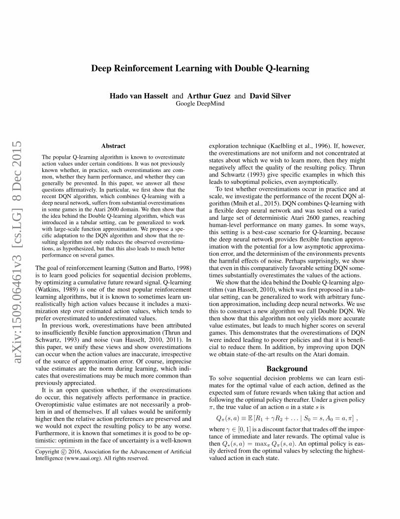
DQN Double DQN Double DQN (tuned)Median 47.5% 88.4% 116.7%Mean 122.0% 273.1% 475.2%

Table 2: Summary of normalized performance up to 30 minutesof play on 49 games with human starts. Results for DQN are fromNair et al. (2015).

to allow for a controlled experiment focused just on re-ducing overestimations. The learned policies are evaluatedfor 5 mins of emulator time (18,000 frames) with an ε-greedy policy where ε = 0.05. The scores are averaged over100 episodes. The only difference between Double DQNand DQN is the target, using Y DoubleDQN

t rather than Y DQN.This evaluation is somewhat adversarial, as the used hyper-parameters were tuned for DQN but not for Double DQN.

To obtain summary statistics across games, we normalizethe score for each game as follows:

scorenormalized =scoreagent − scorerandom

scorehuman − scorerandom. (5)

The ‘random’ and ‘human’ scores are the same as used byMnih et al. (2015), and are given in the appendix.

Table 1, under no ops, shows that on the whole DoubleDQN clearly improves over DQN. A detailed comparison(in appendix) shows that there are several games in whichDouble DQN greatly improves upon DQN. Noteworthy ex-amples include Road Runner (from 233% to 617%), Asterix(from 70% to 180%), Zaxxon (from 54% to 111%), andDouble Dunk (from 17% to 397%).

The Gorila algorithm (Nair et al., 2015), which is a mas-sively distributed version of DQN, is not included in the ta-ble because the architecture and infrastructure is sufficientlydifferent to make a direct comparison unclear. For complete-ness, we note that Gorila obtained median and mean normal-ized scores of 96% and 495%, respectively.

Robustness to Human startsOne concern with the previous evaluation is that in deter-ministic games with a unique starting point the learner couldpotentially learn to remember sequences of actions with-out much need to generalize. While successful, the solutionwould not be particularly robust. By testing the agents fromvarious starting points, we can test whether the found so-lutions generalize well, and as such provide a challengingtestbed for the learned polices (Nair et al., 2015).

We obtained 100 starting points sampled for each gamefrom a human expert’s trajectory, as proposed by Nair et al.(2015). We start an evaluation episode from each of thesestarting points and run the emulator for up to 108,000 frames(30 mins at 60Hz including the trajectory before the startingpoint). Each agent is only evaluated on the rewards accumu-lated after the starting point.

For this evaluation we include a tuned version of DoubleDQN. Some tuning is appropriate because the hyperparame-ters were tuned for DQN, which is a different algorithm. Forthe tuned version of Double DQN, we increased the num-ber of frames between each two copies of the target networkfrom 10,000 to 30,000, to reduce overestimations further be-cause immediately after each switch DQN and Double DQN

0% 100%

200%

300%

400%

500%1000%1500%2000%2500%5000%7500%

Normalized score

Hu

man

∗∗Solaris∗∗Private Eye

GravitarVenture

Montezuma’s RevengeAsteroids

∗∗Pitfall∗∗Ms. Pacman

Amidar∗∗Yars Revenge∗∗

AlienCentipede

Bowling∗∗Skiing∗∗

FrostbiteChopper Command

Seaquest∗∗Berzerk∗∗

H.E.R.O.TutankhamIce Hockey

Battle ZoneRiver Raid

∗∗Surround∗∗Q*BertTennis

Fishing DerbyZaxxon

PongFreeway

Beam RiderBank HeistTime Pilot

Name This GameWizard of WorKung-Fu Master

EnduroJames Bond

Space InvadersUp and Down∗∗Phoenix∗∗∗∗Defender∗∗

AsterixKangaroo

Crazy ClimberKrull

Road RunnerStar Gunner

BoxingGopher

RobotankDouble Dunk

AssaultBreakout

Demon AttackAtlantis

Video Pinball

Double DQN (tuned)

Double DQN

DQN

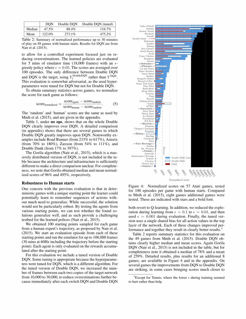
Figure 4: Normalized scores on 57 Atari games, testedfor 100 episodes per game with human starts. Comparedto Mnih et al. (2015), eight games additional games weretested. These are indicated with stars and a bold font.

both revert to Q-learning. In addition, we reduced the explo-ration during learning from ε = 0.1 to ε = 0.01, and thenused ε = 0.001 during evaluation. Finally, the tuned ver-sion uses a single shared bias for all action values in the toplayer of the network. Each of these changes improved per-formance and together they result in clearly better results.3

Table 2 reports summary statistics for this evaluation onthe 49 games from Mnih et al. (2015). Double DQN ob-tains clearly higher median and mean scores. Again GorilaDQN (Nair et al., 2015) is not included in the table, but forcompleteness note it obtained a median of 78% and a meanof 259%. Detailed results, plus results for an additional 8games, are available in Figure 4 and in the appendix. Onseveral games the improvements from DQN to Double DQNare striking, in some cases bringing scores much closer to

3Except for Tennis, where the lower ε during training seemedto hurt rather than help.

human, or even surpassing these.Double DQN appears more robust to this more challeng-

ing evaluation, suggesting that appropriate generalizationsoccur and that the found solutions do not exploit the deter-minism of the environments. This is appealing, as it indi-cates progress towards finding general solutions rather thana deterministic sequence of steps that would be less robust.

DiscussionThis paper has five contributions. First, we have shown whyQ-learning can be overoptimistic in large-scale problems,even if these are deterministic, due to the inherent estima-tion errors of learning. Second, by analyzing the value es-timates on Atari games we have shown that these overesti-mations are more common and severe in practice than pre-viously acknowledged. Third, we have shown that DoubleQ-learning can be used at scale to successfully reduce thisoveroptimism, resulting in more stable and reliable learning.Fourth, we have proposed a specific implementation calledDouble DQN, that uses the existing architecture and deepneural network of the DQN algorithm without requiring ad-ditional networks or parameters. Finally, we have shown thatDouble DQN finds better policies, obtaining new state-of-the-art results on the Atari 2600 domain.

AcknowledgmentsWe would like to thank Tom Schaul, Volodymyr Mnih, MarcBellemare, Thomas Degris, Georg Ostrovski, and RichardSutton for helpful comments, and everyone at Google Deep-Mind for a constructive research environment.

ReferencesR. Agrawal. Sample mean based index policies with O(log n) re-

gret for the multi-armed bandit problem. Advances in AppliedProbability, pages 1054–1078, 1995.

P. Auer, N. Cesa-Bianchi, and P. Fischer. Finite-time analysis of themultiarmed bandit problem. Machine learning, 47(2-3):235–256, 2002.

L. Baird. Residual algorithms: Reinforcement learning with func-tion approximation. In Machine Learning: Proceedings of theTwelfth International Conference, pages 30–37, 1995.

M. G. Bellemare, Y. Naddaf, J. Veness, and M. Bowling. The ar-cade learning environment: An evaluation platform for generalagents. J. Artif. Intell. Res. (JAIR), 47:253–279, 2013.

R. I. Brafman and M. Tennenholtz. R-max-a general polynomialtime algorithm for near-optimal reinforcement learning. TheJournal of Machine Learning Research, 3:213–231, 2003.

K. Fukushima. Neocognitron: A hierarchical neural network ca-pable of visual pattern recognition. Neural networks, 1(2):119–130, 1988.

L. P. Kaelbling, M. L. Littman, and A. W. Moore. Reinforcementlearning: A survey. Journal of Artificial Intelligence Research,4:237–285, 1996.

Y. LeCun, L. Bottou, Y. Bengio, and P. Haffner. Gradient-basedlearning applied to document recognition. Proceedings of theIEEE, 86(11):2278–2324, 1998.

L. Lin. Self-improving reactive agents based on reinforcementlearning, planning and teaching. Machine learning, 8(3):293–321, 1992.

H. R. Maei. Gradient temporal-difference learning algorithms.PhD thesis, University of Alberta, 2011.

V. Mnih, K. Kavukcuoglu, D. Silver, A. A. Rusu, J. Veness, M. G.Bellemare, A. Graves, M. Riedmiller, A. K. Fidjeland, G. Ostro-vski, S. Petersen, C. Beattie, A. Sadik, I. Antonoglou, H. King,D. Kumaran, D. Wierstra, S. Legg, and D. Hassabis. Human-level control through deep reinforcement learning. Nature, 518(7540):529–533, 2015.

A. Nair, P. Srinivasan, S. Blackwell, C. Alcicek, R. Fearon, A. D.Maria, V. Panneershelvam, M. Suleyman, C. Beattie, S. Pe-tersen, S. Legg, V. Mnih, K. Kavukcuoglu, and D. Silver. Mas-sively parallel methods for deep reinforcement learning. In DeepLearning Workshop, ICML, 2015.

M. Riedmiller. Neural fitted Q iteration - first experiences with adata efficient neural reinforcement learning method. In J. Gama,R. Camacho, P. Brazdil, A. Jorge, and L. Torgo, editors, Pro-ceedings of the 16th European Conference on Machine Learning(ECML’05), pages 317–328. Springer, 2005.

B. Sallans and G. E. Hinton. Reinforcement learning with factoredstates and actions. The Journal of Machine Learning Research,5:1063–1088, 2004.

A. L. Strehl, L. Li, and M. L. Littman. Reinforcement learning infinite MDPs: PAC analysis. The Journal of Machine LearningResearch, 10:2413–2444, 2009.

R. S. Sutton. Learning to predict by the methods of temporal dif-ferences. Machine learning, 3(1):9–44, 1988.

R. S. Sutton. Integrated architectures for learning, planning, andreacting based on approximating dynamic programming. InProceedings of the seventh international conference on machinelearning, pages 216–224, 1990.

R. S. Sutton and A. G. Barto. Introduction to reinforcement learn-ing. MIT Press, 1998.

R. S. Sutton, C. Szepesvari, and H. R. Maei. A convergent O(n)algorithm for off-policy temporal-difference learning with lin-ear function approximation. Advances in Neural InformationProcessing Systems 21 (NIPS-08), 21:1609–1616, 2008.

R. S. Sutton, A. R. Mahmood, and M. White. An emphatic ap-proach to the problem of off-policy temporal-difference learn-ing. arXiv preprint arXiv:1503.04269, 2015.

I. Szita and A. Lorincz. The many faces of optimism: a unifyingapproach. In Proceedings of the 25th international conferenceon Machine learning, pages 1048–1055. ACM, 2008.

G. Tesauro. Temporal difference learning and td-gammon. Com-munications of the ACM, 38(3):58–68, 1995.

S. Thrun and A. Schwartz. Issues in using function approxima-tion for reinforcement learning. In M. Mozer, P. Smolensky,D. Touretzky, J. Elman, and A. Weigend, editors, Proceedingsof the 1993 Connectionist Models Summer School, Hillsdale, NJ,1993. Lawrence Erlbaum.

J. N. Tsitsiklis and B. Van Roy. An analysis of temporal-differencelearning with function approximation. IEEE Transactions onAutomatic Control, 42(5):674–690, 1997.

H. van Hasselt. Double Q-learning. Advances in Neural Informa-tion Processing Systems, 23:2613–2621, 2010.

H. van Hasselt. Insights in Reinforcement Learning. PhD thesis,Utrecht University, 2011.

C. J. C. H. Watkins. Learning from delayed rewards. PhD thesis,University of Cambridge England, 1989.

AppendixTheorem 1. Consider a state s in which all the true optimal ac-tion values are equal at Q∗(s, a) = V∗(s) for some V∗(s). LetQt be arbitrary value estimates that are on the whole unbiased inthe sense that

∑a(Qt(s, a) − V∗(s)) = 0, but that are not all

zero, such that 1m

∑a(Qt(s, a) − V∗(s))2 = C for some C > 0,

wherem ≥ 2 is the number of actions in s. Under these conditions,

maxaQt(s, a) ≥ V∗(s) +√

Cm−1

. This lower bound is tight. Un-der the same conditions, the lower bound on the absolute error ofthe Double Q-learning estimate is zero.

Proof of Theorem 1. Define the errors for each action a as εa =Qt(s, a)− V∗(s). Suppose that there exists a setting of {εa} such

that maxa εa <√

Cm−1

. Let {ε+i } be the set of positive ε of size

n, and {ε−j } the set of strictly negative ε of size m − n (suchthat {ε} = {ε+i } ∪ {ε−j }). If n = m, then

∑a εa = 0 =⇒

εa = 0 ∀a, which contradicts∑

a ε2a = mC. Hence, it must be

that n ≤ m − 1. Then,∑n

i=1 ε+i ≤ nmaxi ε

+i < n

√C

m−1,

and therefore (using the constraint∑

a εa = 0) we also have that∑m−nj=1 |ε−j | < n

√C

m−1. This implies maxj |ε−j | < n

√C

m−1. By

Holder’s inequality, then

m−n∑j=1

(ε−j )2 ≤

m−n∑j=1

|ε−j | ·maxj|ε−j |

< n

√C

m− 1n

√C

m− 1.

We can now combine these relations to compute an upper-boundon the sum of squares for all εa:

m∑a=1

(εa)2 =

n∑i=1

(ε+i )2 +

m−n∑j=1

(ε−j )2

< nC

m− 1+ n

√C

m− 1n

√C

m− 1

= Cn(n+ 1)

m− 1

≤ mC.

This contradicts the assumption that∑m

a=1 ε2a < mC, and there-

fore maxa εa ≥√

Cm−1

for all settings of ε that satisfy the con-straints. We can check that the lower-bound is tight by setting

εa =√

Cm−1

for a = 1, . . . ,m − 1 and εm = −√

(m− 1)C.

This verifies∑

a ε2a = mC and

∑a εa = 0.

The only tight lower bound on the absolute error for Double Q-learning |Q′t(s, argmaxaQt(s, a)) − V∗(s)| is zero. This can beseen by because we can have

Qt(s, a1) = V∗(s) +

√Cm− 1

m,

and

Qt(s, ai) = V∗(s)−√C

1

m(m− 1), for i > 1.

Then the conditions of the theorem hold. If then, furthermore, wehave Q′t(s, a1) = V∗(s) then the error is zero. The remaining ac-tion values Q′t(s, ai), for i > 1, are arbitrary.

Theorem 2. Consider a state s in which all the true optimal actionvalues are equal at Q∗(s, a) = V∗(s). Suppose that the estimationerrorsQt(s, a)−Q∗(s, a) are independently distributed uniformlyrandomly in [−1, 1]. Then,

E[max

aQt(s, a)− V∗(s)

]=m− 1

m+ 1

Proof. Define εa = Qt(s, a) − Q∗(s, a); this is a uniform ran-dom variable in [−1, 1]. The probability that maxaQt(s, a) ≤ xfor some x is equal to the probability that εa ≤ x for all a simul-taneously. Because the estimation errors are independent, we canderive

P (maxa

εa ≤ x) = P (X1 ≤ x ∧X2 ≤ x ∧ . . . ∧Xm ≤ x)

=

m∏a=1

P (εa ≤ x) .

The function P (εa ≤ x) is the cumulative distribution function(CDF) of εa, which here is simply defined as

P (εa ≤ x) =

0 if x ≤ −11+x2

if x ∈ (−1, 1)1 if x ≥ 1

This implies that

P (maxa

εa ≤ x) =m∏

a=1

P (εa ≤ x)

=

0 if x ≤ −1(1+x2

)m if x ∈ (−1, 1)1 if x ≥ 1

This gives us the CDF of the random variable maxa εa. Its expec-tation can be written as an integral

E[max

aεa]=

∫ 1

−1

xfmax(x) dx ,

where fmax is the probability density function of this variable, de-fined as the derivative of the CDF: fmax(x) = d

dxP (maxa εa ≤x), so that for x ∈ [−1, 1] we have fmax(x) = m

2

(1+x2

)m−1.Evaluating the integral yields

E[max

aεa]=

∫ 1

−1

xfmax(x) dx

=

[(x+ 1

2

)mmx− 1

m+ 1

]1−1

=m− 1

m+ 1.

Experimental Details for the Atari 2600Domain

We selected the 49 games to match the list used by Mnih et al.(2015), see Tables below for the full list. Each agent step is com-posed of four frames (the last selected action is repeated duringthese frames) and reward values (obtained from the Arcade Learn-ing Environment (Bellemare et al., 2013)) are clipped between -1and 1.

Network ArchitectureThe convolution network used in the experiment is exactly the oneproposed by proposed by Mnih et al. (2015), we only provide de-tails here for completeness. The input to the network is a 84x84x4tensor containing a rescaled, and gray-scale, version of the last fourframes. The first convolution layer convolves the input with 32 fil-ters of size 8 (stride 4), the second layer has 64 layers of size 4(stride 2), the final convolution layer has 64 filters of size 3 (stride1). This is followed by a fully-connected hidden layer of 512 units.All these layers are separated by Rectifier Linear Units (ReLu). Fi-nally, a fully-connected linear layer projects to the output of thenetwork, i.e., the Q-values. The optimization employed to train thenetwork is RMSProp (with momentum parameter 0.95).

Hyper-parametersIn all experiments, the discount was set to γ = 0.99, and the learn-ing rate to α = 0.00025. The number of steps between target net-work updates was τ = 10, 000. Training is done over 50M steps(i.e., 200M frames). The agent is evaluated every 1M steps, andthe best policy across these evaluations is kept as the output of thelearning process. The size of the experience replay memory is 1Mtuples. The memory gets sampled to update the network every 4steps with minibatches of size 32. The simple exploration policyused is an ε-greedy policy with the ε decreasing linearly from 1 to0.1 over 1M steps.

Supplementary Results in the Atari 2600Domain

The Tables below provide further detailed results for our experi-ments in the Atari domain.

Game Random Human DQN Double DQNAlien 227.80 6875.40 3069.33 2907.30Amidar 5.80 1675.80 739.50 702.10Assault 222.40 1496.40 3358.63 5022.90Asterix 210.00 8503.30 6011.67 15150.00Asteroids 719.10 13156.70 1629.33 930.60Atlantis 12850.00 29028.10 85950.00 64758.00Bank Heist 14.20 734.40 429.67 728.30Battle Zone 2360.00 37800.00 26300.00 25730.00Beam Rider 363.90 5774.70 6845.93 7654.00Bowling 23.10 154.80 42.40 70.50Boxing 0.10 4.30 71.83 81.70Breakout 1.70 31.80 401.20 375.00Centipede 2090.90 11963.20 8309.40 4139.40Chopper Command 811.00 9881.80 6686.67 4653.00Crazy Climber 10780.50 35410.50 114103.33 101874.00Demon Attack 152.10 3401.30 9711.17 9711.90Double Dunk -18.60 -15.50 -18.07 -6.30Enduro 0.00 309.60 301.77 319.50Fishing Derby -91.70 5.50 -0.80 20.30Freeway 0.00 29.60 30.30 31.80Frostbite 65.20 4334.70 328.33 241.50Gopher 257.60 2321.00 8520.00 8215.40Gravitar 173.00 2672.00 306.67 170.50H.E.R.O. 1027.00 25762.50 19950.33 20357.00Ice Hockey -11.20 0.90 -1.60 -2.40James Bond 29.00 406.70 576.67 438.00Kangaroo 52.00 3035.00 6740.00 13651.00Krull 1598.00 2394.60 3804.67 4396.70Kung-Fu Master 258.50 22736.20 23270.00 29486.00Montezuma’s Revenge 0.00 4366.70 0.00 0.00Ms. Pacman 307.30 15693.40 2311.00 3210.00Name This Game 2292.30 4076.20 7256.67 6997.10Pong -20.70 9.30 18.90 21.00Private Eye 24.90 69571.30 1787.57 670.10Q*Bert 163.90 13455.00 10595.83 14875.00River Raid 1338.50 13513.30 8315.67 12015.30Road Runner 11.50 7845.00 18256.67 48377.00Robotank 2.20 11.90 51.57 46.70Seaquest 68.40 20181.80 5286.00 7995.00Space Invaders 148.00 1652.30 1975.50 3154.60Star Gunner 664.00 10250.00 57996.67 65188.00Tennis -23.80 -8.90 -2.47 1.70Time Pilot 3568.00 5925.00 5946.67 7964.00Tutankham 11.40 167.60 186.70 190.60Up and Down 533.40 9082.00 8456.33 16769.90Venture 0.00 1187.50 380.00 93.00Video Pinball 16256.90 17297.60 42684.07 70009.00Wizard of Wor 563.50 4756.50 3393.33 5204.00Zaxxon 32.50 9173.30 4976.67 10182.00

Table 3: Raw scores for the no-op evaluation condition (5 minutes emulator time). DQN as given by Mnih et al. (2015).

Game DQN Double DQNAlien 42.75 % 40.31 %Amidar 43.93 % 41.69 %Assault 246.17 % 376.81 %Asterix 69.96 % 180.15 %Asteroids 7.32 % 1.70 %Atlantis 451.85 % 320.85 %Bank Heist 57.69 % 99.15 %Battle Zone 67.55 % 65.94 %Beam Rider 119.80 % 134.73 %Bowling 14.65 % 35.99 %Boxing 1707.86 % 1942.86 %Breakout 1327.24 % 1240.20 %Centipede 62.99 % 20.75 %Chopper Command 64.78 % 42.36 %Crazy Climber 419.50 % 369.85 %Demon Attack 294.20 % 294.22 %Double Dunk 17.10 % 396.77 %Enduro 97.47 % 103.20 %Fishing Derby 93.52 % 115.23 %Freeway 102.36 % 107.43 %Frostbite 6.16 % 4.13 %Gopher 400.43 % 385.66 %Gravitar 5.35 % -0.10 %H.E.R.O. 76.50 % 78.15 %Ice Hockey 79.34 % 72.73 %James Bond 145.00 % 108.29 %Kangaroo 224.20 % 455.88 %Krull 277.01 % 351.33 %Kung-Fu Master 102.37 % 130.03 %Montezuma’s Revenge 0.00 % 0.00 %Ms. Pacman 13.02 % 18.87 %Name This Game 278.29 % 263.74 %Pong 132.00 % 139.00 %Private Eye 2.53 % 0.93 %Q*Bert 78.49 % 110.68 %River Raid 57.31 % 87.70 %Road Runner 232.91 % 617.42 %Robotank 508.97 % 458.76 %Seaquest 25.94 % 39.41 %Space Invaders 121.49 % 199.87 %Star Gunner 598.09 % 673.11 %Tennis 143.15 % 171.14 %Time Pilot 100.92 % 186.51 %Tutankham 112.23 % 114.72 %Up and Down 92.68 % 189.93 %Venture 32.00 % 7.83 %Video Pinball 2539.36 % 5164.99 %Wizard of Wor 67.49 % 110.67 %Zaxxon 54.09 % 111.04 %

Table 4: Normalized results for no-op evaluation condition (5 minutes emulator time).

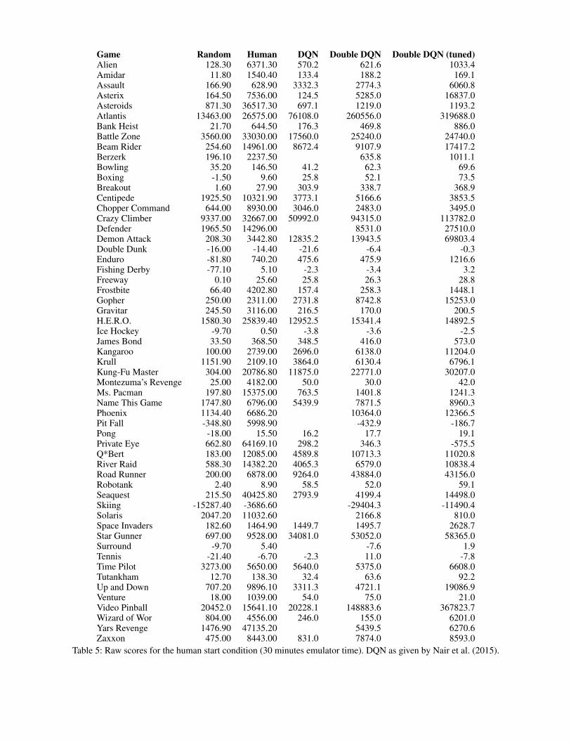
Game Random Human DQN Double DQN Double DQN (tuned)Alien 128.30 6371.30 570.2 621.6 1033.4Amidar 11.80 1540.40 133.4 188.2 169.1Assault 166.90 628.90 3332.3 2774.3 6060.8Asterix 164.50 7536.00 124.5 5285.0 16837.0Asteroids 871.30 36517.30 697.1 1219.0 1193.2Atlantis 13463.00 26575.00 76108.0 260556.0 319688.0Bank Heist 21.70 644.50 176.3 469.8 886.0Battle Zone 3560.00 33030.00 17560.0 25240.0 24740.0Beam Rider 254.60 14961.00 8672.4 9107.9 17417.2Berzerk 196.10 2237.50 635.8 1011.1Bowling 35.20 146.50 41.2 62.3 69.6Boxing -1.50 9.60 25.8 52.1 73.5Breakout 1.60 27.90 303.9 338.7 368.9Centipede 1925.50 10321.90 3773.1 5166.6 3853.5Chopper Command 644.00 8930.00 3046.0 2483.0 3495.0Crazy Climber 9337.00 32667.00 50992.0 94315.0 113782.0Defender 1965.50 14296.00 8531.0 27510.0Demon Attack 208.30 3442.80 12835.2 13943.5 69803.4Double Dunk -16.00 -14.40 -21.6 -6.4 -0.3Enduro -81.80 740.20 475.6 475.9 1216.6Fishing Derby -77.10 5.10 -2.3 -3.4 3.2Freeway 0.10 25.60 25.8 26.3 28.8Frostbite 66.40 4202.80 157.4 258.3 1448.1Gopher 250.00 2311.00 2731.8 8742.8 15253.0Gravitar 245.50 3116.00 216.5 170.0 200.5H.E.R.O. 1580.30 25839.40 12952.5 15341.4 14892.5Ice Hockey -9.70 0.50 -3.8 -3.6 -2.5James Bond 33.50 368.50 348.5 416.0 573.0Kangaroo 100.00 2739.00 2696.0 6138.0 11204.0Krull 1151.90 2109.10 3864.0 6130.4 6796.1Kung-Fu Master 304.00 20786.80 11875.0 22771.0 30207.0Montezuma’s Revenge 25.00 4182.00 50.0 30.0 42.0Ms. Pacman 197.80 15375.00 763.5 1401.8 1241.3Name This Game 1747.80 6796.00 5439.9 7871.5 8960.3Phoenix 1134.40 6686.20 10364.0 12366.5Pit Fall -348.80 5998.90 -432.9 -186.7Pong -18.00 15.50 16.2 17.7 19.1Private Eye 662.80 64169.10 298.2 346.3 -575.5Q*Bert 183.00 12085.00 4589.8 10713.3 11020.8River Raid 588.30 14382.20 4065.3 6579.0 10838.4Road Runner 200.00 6878.00 9264.0 43884.0 43156.0Robotank 2.40 8.90 58.5 52.0 59.1Seaquest 215.50 40425.80 2793.9 4199.4 14498.0Skiing -15287.40 -3686.60 -29404.3 -11490.4Solaris 2047.20 11032.60 2166.8 810.0Space Invaders 182.60 1464.90 1449.7 1495.7 2628.7Star Gunner 697.00 9528.00 34081.0 53052.0 58365.0Surround -9.70 5.40 -7.6 1.9Tennis -21.40 -6.70 -2.3 11.0 -7.8Time Pilot 3273.00 5650.00 5640.0 5375.0 6608.0Tutankham 12.70 138.30 32.4 63.6 92.2Up and Down 707.20 9896.10 3311.3 4721.1 19086.9Venture 18.00 1039.00 54.0 75.0 21.0Video Pinball 20452.0 15641.10 20228.1 148883.6 367823.7Wizard of Wor 804.00 4556.00 246.0 155.0 6201.0Yars Revenge 1476.90 47135.20 5439.5 6270.6Zaxxon 475.00 8443.00 831.0 7874.0 8593.0

Table 5: Raw scores for the human start condition (30 minutes emulator time). DQN as given by Nair et al. (2015).

Game DQN Double DQN Double DQN (tuned)Alien 7.08% 7.90% 14.50%Amidar 7.95% 11.54% 10.29%Assault 685.15% 564.37% 1275.74%Asterix -0.54% 69.46% 226.18%Asteroids -0.49% 0.98% 0.90%Atlantis 477.77% 1884.48% 2335.46%Bank Heist 24.82% 71.95% 138.78%Battle Zone 47.51% 73.57% 71.87%Beam Rider 57.24% 60.20% 116.70%Berzerk 21.54% 39.92%Bowling 5.39% 24.35% 30.91%Boxing 245.95% 482.88% 675.68%Breakout 1149.43% 1281.75% 1396.58%Centipede 22.00% 38.60% 22.96%Chopper Command 28.99% 22.19% 34.41%Crazy Climber 178.55% 364.24% 447.69%Defender 53.25% 207.17%Demon Attack 390.38% 424.65% 2151.65%Double Dunk -350.00% 600.00% 981.25%Enduro 67.81% 67.85% 157.96%Fishing Derby 91.00% 89.66% 97.69%Freeway 100.78% 102.75% 112.55%Frostbite 2.20% 4.64% 33.40%Gopher 120.42% 412.07% 727.95%Gravitar -1.01% -2.63% -1.57%H.E.R.O. 46.88% 56.73% 54.88%Ice Hockey 57.84% 59.80% 70.59%James Bond 94.03% 114.18% 161.04%Kangaroo 98.37% 228.80% 420.77%Krull 283.34% 520.11% 589.66%Kung-Fu Master 56.49% 109.69% 145.99%Montezuma’s Revenge 0.60% 0.12% 0.41%Ms. Pacman 3.73% 7.93% 6.88%Name This Game 73.14% 121.30% 142.87%Phoenix 166.25% 202.31%Pit Fall -1.32% 2.55%Pong 102.09% 106.57% 110.75%Private Eye -0.57% -0.50% -1.95%Q*Bert 37.03% 88.48% 91.06%River Raid 25.21% 43.43% 74.31%Road Runner 135.73% 654.15% 643.25%Robotank 863.08% 763.08% 872.31%Seaquest 6.41% 9.91% 35.52%Skiing -121.69% 32.73%Solaris 1.33% -13.77%Space Invaders 98.81% 102.40% 190.76%Star Gunner 378.03% 592.85% 653.02%Surround 13.91% 76.82%Tennis 129.93% 220.41% 92.52%Time Pilot 99.58% 88.43% 140.30%Tutankham 15.68% 40.53% 63.30%Up and Down 28.34% 43.68% 200.02%Venture 3.53% 5.58% 0.29%Video Pinball -4.65% 2669.60% 7220.51%Wizard of Wor -14.87% -17.30% 143.84%Yars Revenge 8.68% 10.50%Zaxxon 4.47% 92.86% 101.88%

Table 6: Normalized scores for the human start condition (30 minutes emulator time).