Mesh generation for SCHISM with SMS:with focus on compound flooding

VIMS and DWR teams

1

The good news and bad news• Bad news

• UG grid generation is often a laborious and iterative process

• Steepest part of the learning curve for UG models (and each model has its own secret recipe)

• This is especially true for very large grids: a common source of frustration with SMS – build confidence gradually

• Good news

• SCHISM is not picky about grid quality (for triangles); won’t blow up easily

• Once you master the M.G., the rest of the model setup is more straightforward

• A few ways to blow up the model

• Bad quality quads: split them to get pair of triangles (there is a FORTRAN util script for this)

• Violation of inverse CFL criterion (CFL>0.4)

• Dry open boundary: newer versions allow this, but still do not allow the entire segment to become dry if you impose velocity/discharge there

• Momentum dissipation too low

2

Tools

• Recommend SMS, using “conceptual maps”– Good advantage of terrain– Patch/pave comparison– Bugs, high level of manual work (so save along the way)

• Triangle is a good free product– Driven mostly by exterior (2D shore)

• Janet: expensive, orthogonality not needed• DistMesh: Beautiful introduction to density functions, curvature. Not all the good stuff is

in the software.• STOMEL (Holleman et al 2013): Flow-aligned mesh and numerical diffusion, but

orthogonal• GMESH, JIGSAW…• Fully automatic, DEM-driven tools: oceanmesh2D, geomesh

3

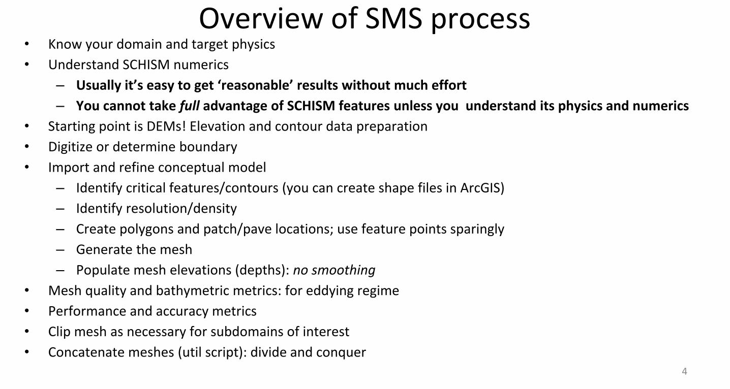
Overview of SMS process• Know your domain and target physics

• Understand SCHISM numerics

– Usually it’s easy to get ‘reasonable’ results without much effort

– You cannot take full advantage of SCHISM features unless you understand its physics and numerics

• Starting point is DEMs! Elevation and contour data preparation

• Digitize or determine boundary

• Import and refine conceptual model

– Identify critical features/contours (you can create shape files in ArcGIS)

– Identify resolution/density

– Create polygons and patch/pave locations; use feature points sparingly

– Generate the mesh

– Populate mesh elevations (depths): no smoothing

• Mesh quality and bathymetric metrics: for eddying regime

• Performance and accuracy metrics

• Clip mesh as necessary for subdomains of interest

• Concatenate meshes (util script): divide and conquer4

Next step

• Generate mesh in SMS

– Need to specify meshing types (patch, paving) in polygons

– Generate mesh

– Remember to ‘Select disjoint’ (under Nodes menu) and remove disjoint nodes

– ‘Renumber’ (under Nodes) as an added safety measure

– Can use lon/lat as long as the tolerance is set properly

– Proceed to other model setup (pre-processor) steps: SCHISM’s pre-processor is very good at catching meshing errors

SCHISM Bay-Delta and Bay Subdomain

Bay SCHISM

Bay-Delta SCHISM:~180,000 nodes~360,000 elements

6

7

South Delta Temporary Barriers

Clifton Court

ForebayUnion Island

Roberts

IslandJones

Tract

Fabian Tract

Head of Old RiverMiddle RiverGrant Line Canal

Old River at Tracy

Stockton●

Delta

• Channelized, levees• Levees and “islands”• 3D challenges beyond estuary processes• Extensive tidal influence

8

Estuary Transport (3D)

9

SMS Resources

• SMS/Aquaveo website

• Todd Wood Masters Thesis:

– Can be viewed from wiki (www.schism.wiki)

– Very good step-by-step

– Honest account of debugging such as “bisection” to find bad spots

10

General rules• Unlike explicit models, you’ll find M.G. for SCHISM is more ‘intuitive’ and

‘freer’– Implicit model allows you to focus on physics instead of numerics

– You are freer to resolve important features without worrying about cost/instability

– SCHISM is not picky about mesh quality (except for quads); however, mesh quality pays off for accuracy especially in some critical regions

– M.G. for complex applications requires more effort; often an iterative process: establishing a good workflow is essential so you can redo

– Remember the starting point is DEMs!

– Mesh for 3D model needs to be relatively smooth in eddying and transitional regimes, in order to not distort eddy kinetics (Wang and Danilov 2016): this is an important issue when we get to 3D model

11

SMS Conceptual Model

12• Nodes, vertices, arcs and polygons

DEM preparation: pre-filtering bathymetry

• Unresolved subgrid features may be eliminated– eliminates lunar landscape undulations on mudflats

– level set or active contour methods (e.g. Malladi and Sethian): contours conservatively straighten

– California DWR has python code smooth_contour.py for small regions

– This is mainly to assist in the arc creation, less for actual interpolation of depths

13

Liberty Island Smoothing:

Malladi and Sethian Min-max curvature flow 14

Wetting and Drying in the Frontal Direction can create “waterfalls”

• Undulating channel creating waterfalls• Can either improve the resolution or keep this in mind when interpreting the results

15

..on the other hand, lateral inundation is smoother

Generating Contour Shapefiles

• ArcGIS allows graphical cleaning• GDAL (gdal_contour) is free and good for quick manipulation

on-the-fly• SMS sister product WMS has some contour tools• All use bilinear interpolation• Note that SMS < 11.1 has a georeferencing mistake for

contours (cell- vs vertex-centered) • Python shapefile library very useful for exporting arcs based

on calculations in (x,y)

16

Visualizing Contours

• SMS has very limited memory

• You can use a coarse tin or DEM for conceptual visualization or on small domains

• clip_dem.py allows tailored geographical information

17

Cleaning

• Snapping vertices

• Intersecting arcs

• Dangling arcs

• Mixed feelings about them all: if you change default, you may be at risk of unexplained crashes

18

Magic Contours

• Foot/top of slope, thalweg

• High-gradient zone in DEM for ‘features’

• Shoreline and probable “real” water levels (to initialize wet/dry)

• Flooding and mudflats: throw in extra resolution helps if you can afford it

• Key features (jetty, breakwater…): be game!

• TVD (h_tvd) and other algorithm switches

• Depths used in friction and other user threshold choices

• No need to be 100% conformant; key is to capture features

19

h_tvd = 5m,Water elev ~ 0.5m so -4.0 NAVD contour mostly non-TVD

ChannelShoal

Tidal range

Skew elements

20

Choose Connected Contours

Changing from -2 to -3m increases connectivityNo need to be religious about following contours exactly

Well resolved without help

21

Choose Smoother Deep Contours

22

Stick with the center

Ignores inner

channel

Follows inner channel

without helpInner channel

delineated

23• Accounting for interpolation errors, you can err on each side of wet vs dry

• For choke points of channel, you may want to ensure the “wet” portion is captured by placing the arcs slightly inside the channel line

Grid Density• Need guidance from inverse CFL>0.4

– Start from a smallest expected Δt (e.g., 100s)– Use CFL>0.4 to back calculate the coarsest Δx at a given depth

• Deeper regions generally coarser than shallows but not always (compare this with explicit models which are constrained by CFL)– Often channel needs to be resolved for accurate tracer transport (high

gradients)

• Curvature should be resolved for accurate tidal propagation– 2D: bend in shorelines– 3D: changes in slope (vertical grid plays a role)

• Width of features (sills, beaches, channels)– Skeletonization algorithms (see Per-Olof Persson dissertation)

24

Δt=100s (expected minimum*)

* Remember to recheck CFL if for some reason you have to reduce Δt* Small patches of violation is fine especially near shoreline; avoid large areas in open area

Grid resolution Guide

Control Grid Density In SMS

• Density-based paving• Shore resolution propagates in• Refinement nodes (node in map tool) can enforce local

resolution (but may produce skew elements or even disjoint nodes)

26

Wetting and Drying• Element-based designation

– Based on node elevations

– All 3|4 wet => wet element

– No partial wet/dry

• Velocities calculated on edges of wet elements

27

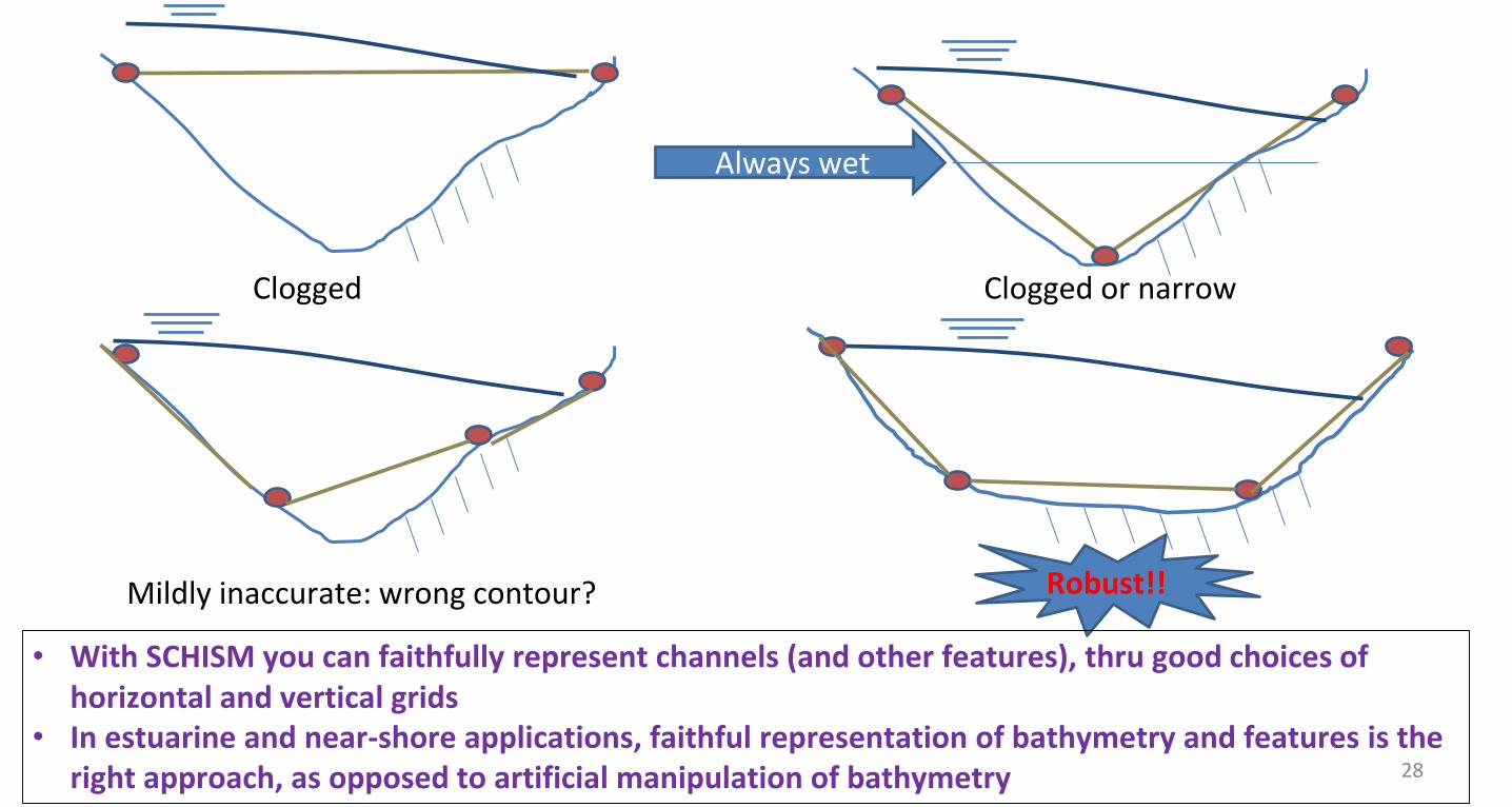
Always wet

Clogged Clogged or narrow

Mildly inaccurate: wrong contour? Robust!!

• With SCHISM you can faithfully represent channels (and other features), thru good choices of horizontal and vertical grids

• In estuarine and near-shore applications, faithful representation of bathymetry and features is the right approach, as opposed to artificial manipulation of bathymetry 28

Patching and Paving

Patch

Pave

29

Mesh Types (Patch vs Paving)

30

• Older versions of SMS used to be a pain for keeping track of patches; newer versions are better

• Bias easier to “undo” here• Make sure there are only 4 corner nodes (merge some if necessary)

31

Patch vs PavePave:- Recommended for quality grids on large, well-resolved water bodies- Works well when polygon is big and wide compared to arc nodes- Most robust of all methods- Resolution harder to control in the interior

32

33

(Adaptive) Coon’s Patch• Quasi-structured grid block

• Force mesh to be n-elements wide (good idea to try to match on opposite boundaries)

• Arbitrary anisotropy (3:1 or 4:1 common)

• Follow the channel!!! Don’t round corners

• Easier to control cross-channel resolutionPatch (Adaptive Coon’s Patch)

Pave (advancing front)

34

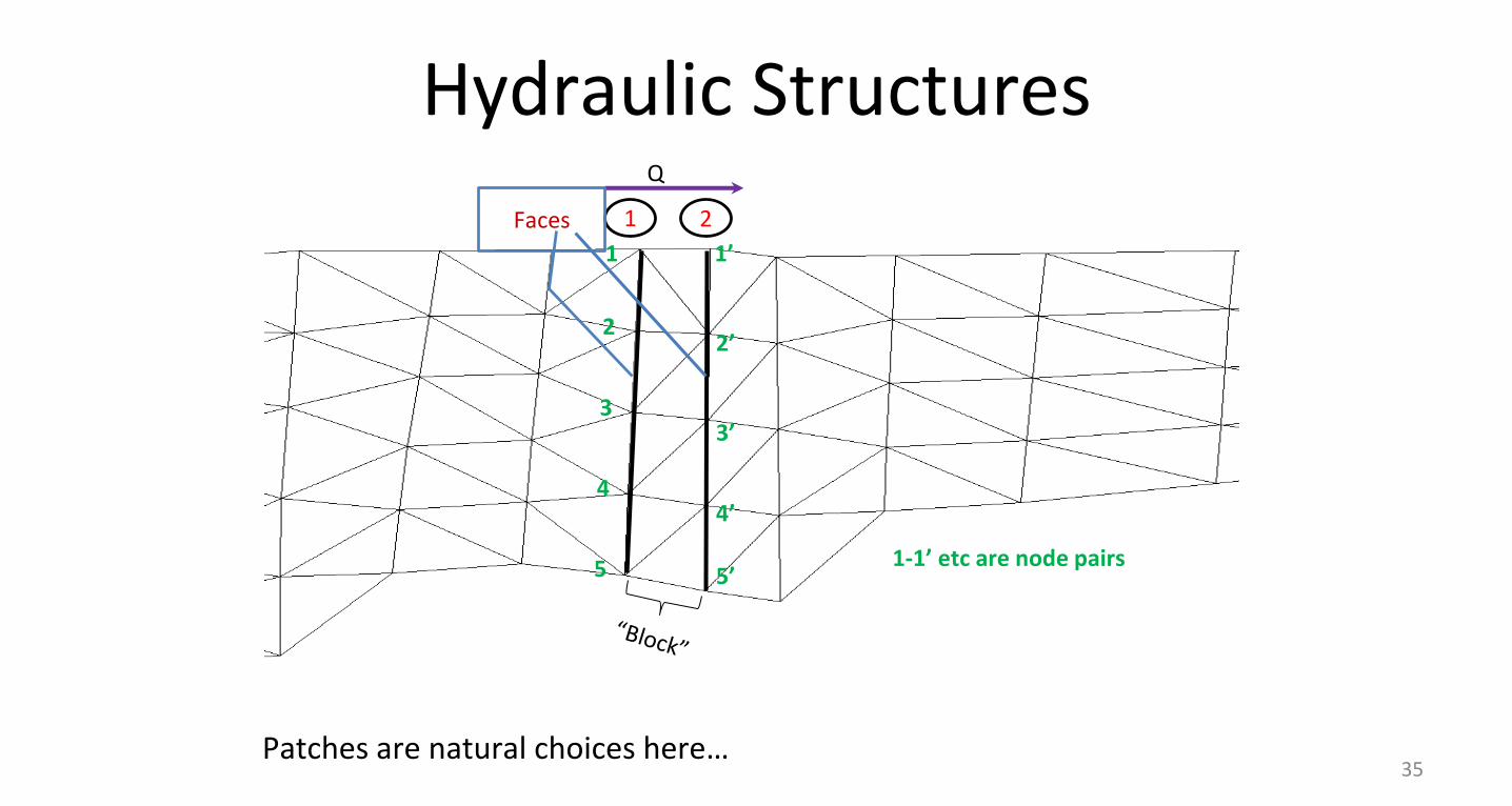
Hydraulic Structures

1 2

Q

Faces

1

2

3

4

5 5’

4’

3’

2’

1’

1-1’ etc are node pairs

35Patches are natural choices here…

Dovetailing Patch and Pave*

*These ideas not unique to patch/pave

36*Note the change in effective resolution…

Populating Elevations• Big problem again … SMS doesn’t hold the data gracefully

• Have heard of people doing it in stages

• Can use stacked_dem_fill.py, which:– Populates with correct georeference

– Matches contours

– Uses prioritized DEMs

– Gives some warnings

• We also have FORTRAN scripts for loading very large TIN (UG) or raster DEMs

• We always use linear interpolation (consistent with SCHISM’s shape function), without any smoothing– You should always visualize the bathymetry immediately after M.G.; correct mistakes

(e.g. blocked channels) immediately37

Metrics• Volumetric error (actually, average height)

– Patterns can be systematic (DWR has tools)

• Face/edge aperture or area

• Storage area

• Skew: SCHISM very tolerant, but good to look for “collapsed” elements (if you use xmgredit5, try skewness of 14)

• Need to use quality quads (use util to automatically split bad quads for you)

• Area change: SCHISM very tolerant

• Slope: PGE issue usually not a problem with parameter choices; vgrid plays a role also

• Local error: Richardson extrapolation

– Painful without tools

• TVD2 and sub-cycling measures (subcycling.out; dtbe outputs): efficiency consideration; can use ielm_transport to mitigate

• Eddying regime requires more uniform and higher-quality grid to avoid distortion of eddy dynamics

• CFL (>0.4)

– Use xmgredit5 to check CFL

– Dimensionless wave number may also need to be looked at38

Automatic regrid/subgrid

39

…it’s generally easier (and quicker) to regrid the whole grid

Common Ad Hoc Fixup Steps

• Deepening of boundary depths to prevent open boundary drying

• No longer necessary in newer versions

40

In gredit, create a region and e.g., depth=max(depth,3)

Conclusions• SMS is an adequate tool for non-orthogonal grids• Good mesh generation resolves flow/bathy features faithfully

– Some finer scales ignored if not resolved– Implicit FE model provides you with more freedom for resolution

• Shape functions and wet-dry rules; understand the physics and numerics • You can’t work on this stuff unless you can fix-test-fix-test

– So front-end on node-based inputs (see BayDeltaSCHISM)

• IMPORTANT: always start from an estimate of smallest Δt you anticipate for the application and use CFL>0.4 to back-calculate the coarsest resolution at each depth– If you somehow decide to reduce Δt later, you may have to refine the grid– As a rough guide, Δt=100-450s for b-tropic, 100-200s for b-clinic applications

(however, smaller Δt might be needed for some extreme cases)

41

42

Compound flooding

Steps in preparing ‘maps’ for SMS mesh generation

1. Generate coastlines and land boundary2. Resolve major river channels3. Resolve levees (and other important

features)4. Add NWM segments into map

NOAA_CRM (3 arc-s, 90m)https://maps.ngdc.noaa.gov/viewers/bathymetry/?layers=dem

• Load DEMs from NOAA CRM, ~90m resolution. There are 5 pieces of CRM files available covering east coast and GOMx regions: (https://maps.ngdc.noaa.gov/viewers/bathymetry/?layers=dem)

• Extract 0m contour as coastline (which will be revised later) and 10m contour as land boundary

1. Generate coastlines and land boundaries

• Use GIS tools to simplify or clean the contours to remove unresolved small features

• Copy some cleaned lines from the existing shape files and work on them as a new layer– Use "Select Feature" button in QGIS to select the feature arc, and then copy and paste it in a

new layer.

1. Generate coastlines and land boundaries

• Load the coastline and land boundary into SMS

• In open ocean, go easy on grid resolution transition (which is important for 3D applications): please refer to Chapter 5.7.1 in the user manual

• Convert the shape file into “feature arcs” and reset the resolution to desired value using “redistribute arcs” option– Land boundary: ~300m– Shoreline: 200m-1km without

estuaries; variable inside estuaries (finer upstream)

1. Generate coastlines and land boundaries

• Download relevant higher resolution DEMs to extract contour lines in a region

USGS_CoNED (1m, nav1983, navd 88)https://topotools.cr.usgs.gov/topobathy_viewer/

2. Resolve river channels and major creeks

• Contour values extracted should be dictated by the specific river channel depths and side slopes

• For estuaries in coastal zones, contours from 5-30m below water are usually used to detect the highest bathymetric gradients

• For river channels and creeks in watershed, contours from 1-5 m below water or sometimes 0m-10m above water may be extracted to help detect the thalwegs– Imageries are helpful also

• Quads (patches) are useful to ensure adequate cross-channel resolution– This entails some manual work

2. Resolve river channels and major creeks

• For coastal estuaries, extract contours of 5m-30m depths below water (-30m ~ -5m from DEMs) to help identify river channels

• Resample using “Simplify Line” to reset the resolution of contour to 10m, to reduce the size of the shape files in GIS

• Use these contours as guidance to resolve river channels in SMS

2. Resolve river channels and major creeks

• If desired, for watershed rivers/creeks, extract 1m to 10m above MSL to help identify thalwegs of creeks• Set along-channel resolution to be 50-300m (finer upstream)• Cross-channel resolution varies from upstream to downstream and also depends on 2D/3D config

– Generally, use at least 5 cross-channel segments in regions with important 3D processes (e.g. stratification)– Otherwise, 1-2 rows of elements are sufficient

2. Resolve river channels and major creeks

• Levee shape files can be found by following website:– https://levees.sec.usace.army.mil/#/

3. Resolve levees and other features

• Extract 1-8m above MSL contour lines from DEMs to help identify bottom and top of levee

• Select the most relevant contour lines and save as new shape file in QGIS

3. Resolve levees and other features

• Take levees in lower Mississippi River as an example, use 4-5m isotopo to trace the top of levees, and use 2m isotopo as the bottom of levees.

• For lower Mississippi, levees in some southern parts of river are lower than 2m, not all connected, and hard to tell from the imagery. So this part is not included at the moment

• For northern parts, elevation is higher, use 9m or 8m contour as the bottom of levees, and use 10m contour to trace the top of levees.

• Before loading the contours into SMS, simplify contours by selecting clean contours in GIS tools, reset the line resolution (~10m) to reduce size, and save them as new shape files

3. Resolving levees and other features

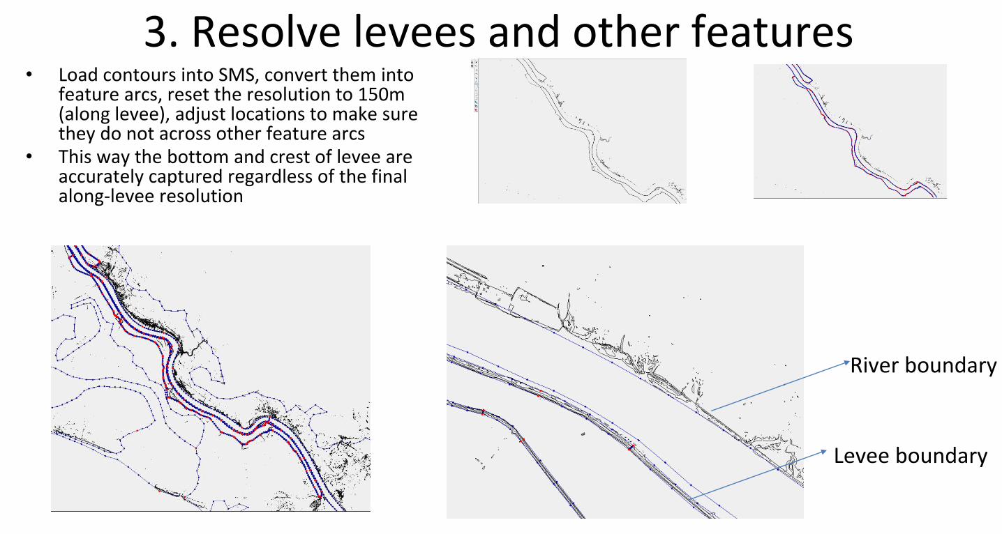
• Load contours into SMS, convert them into feature arcs, reset the resolution to 150m (along levee), adjust locations to make sure they do not across other feature arcs

• This way the bottom and crest of levee are accurately captured regardless of the final along-levee resolution

3. Resolve levees and other features

River boundary

Levee boundary

• Use satellite imagery to edit levee arcs when there is mismatch between DEMs and imagery

3. Resolve levees and other features

Levees

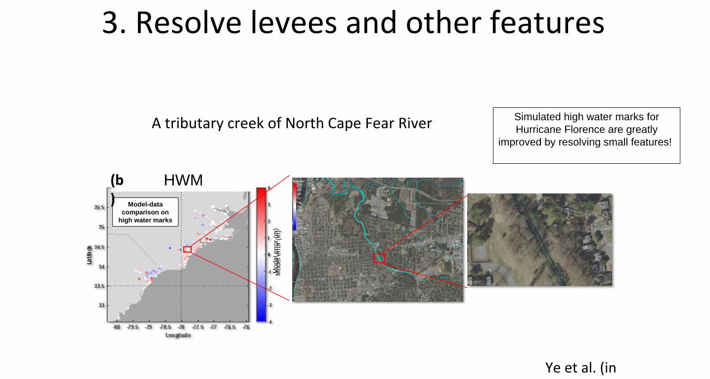
A tributary creek of North Cape Fear River

3. Resolve levees and other features

Simulated high water marks for

Hurricane Florence are greatly

improved by resolving small features!

Model err

or

(m)

Glider deployment:

model-data comparison

on hurricane mixing

HWM

Model-data

comparison on

high water marks

Model err

or

(m)

(b)

Ye et al. (in review)

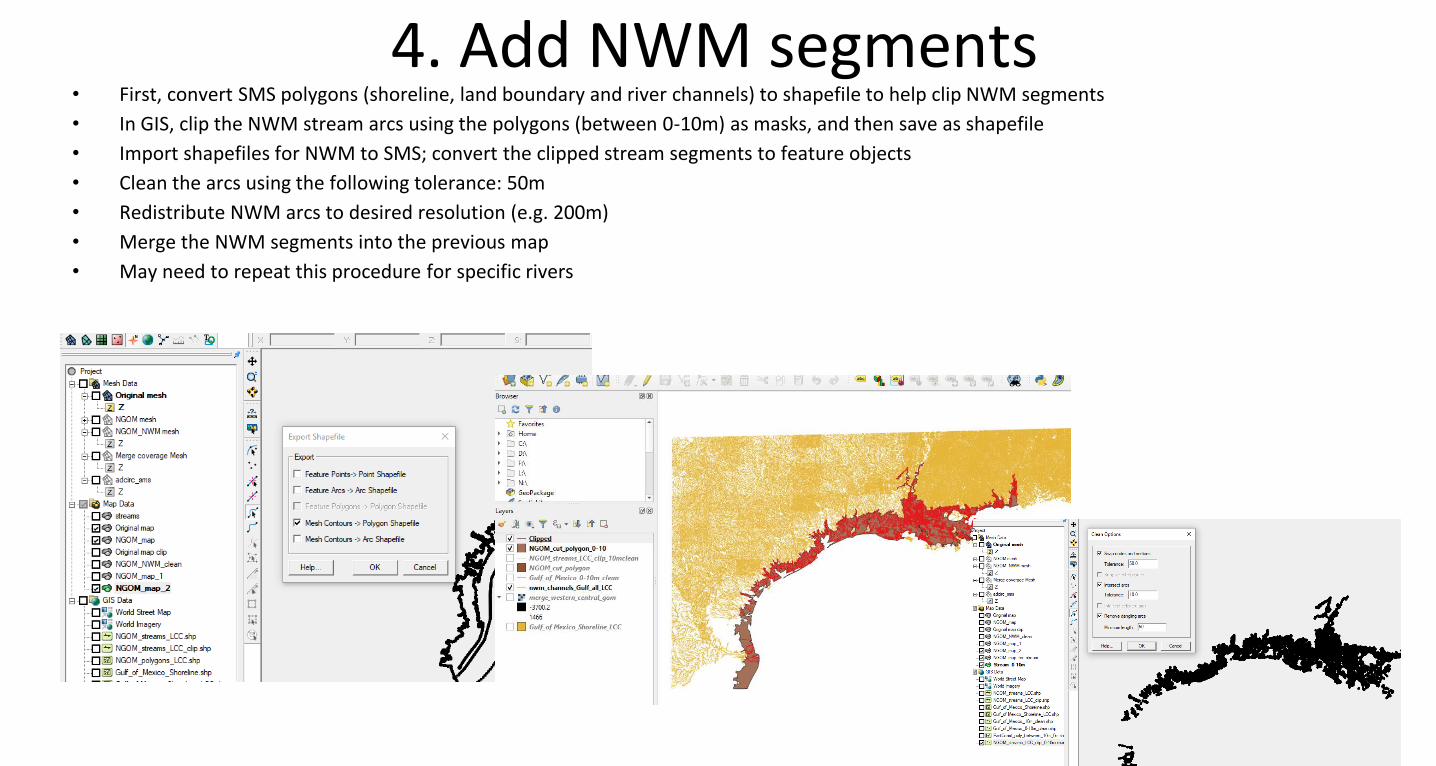
• First, convert SMS polygons (shoreline, land boundary and river channels) to shapefile to help clip NWM segments

• In GIS, clip the NWM stream arcs using the polygons (between 0-10m) as masks, and then save as shapefile

• Import shapefiles for NWM to SMS; convert the clipped stream segments to feature objects

• Clean the arcs using the following tolerance: 50m

• Redistribute NWM arcs to desired resolution (e.g. 200m)

• Merge the NWM segments into the previous map

• May need to repeat this procedure for specific rivers

4. Add NWM segments

• Open the two shape files: channels.shp and watershed_SC.shp in ArcMap software• Use the “buffer” tool to define a zone so that the interested area and the channels do not overlap

4. Some tips on merging NWM arcs

• Use “erase” tool to erase the NWM arcs inside our river polygons (where we have manually aligned channels)

• Obtain the watershed_SC_Erase in which the NWM arcs in the channels_Buffer have been excluded

4. Some tips on merging NWM arcs

• Load the watershed_SC_arcmap.shp into SMS

• Convert it to a feature object by creating a separate new map coverage called watershed_SC_Erase

4. Some tips on merging NWM arcs

• Merge the channels and the watershed_SC_Erase into one map file• Then you will have a newly merged map as shown below, which is the semi-final map

that has everything in it

4. Some tips on merging NWM arcs

• In GIS, clean the small hanging arcs (i.e. not attached to major streams) if desired• Extract the intersections using "Line intersections" tool• Select the arcs using "Select by locations" so that hanging arcs will be excluded• Then invert the selection, copy the selection, and paste it to a new layer: Green color

(hanging arcs) will be excluded

4. Some tips on merging NWM arcs