1

Using SCHISM

Joseph Zhang

2Primer

Online manual and wiki resource: www.schism.wikio There are beta_notes, sample files etc in each source code bundle

It helps if you know a few programming/scripting languages: python, matlab, FORTRAN etc for pre- and post-processing needs

‘Bare minimum’: mandatory inputs Generate a hgrid.gr3 with simplest possible b.c. (e.g., no open bnd) Run SCHISM in 2D config: manning.gr3, param.nml, bctides.in, vgrid.in (2

levels) Pre-processing with ipre=1 first (with 1 CPU) to catch grid and other issues Then proceed to more complex set-ups Establish a good work flow and be willing to revise the grid

3Sample run directory

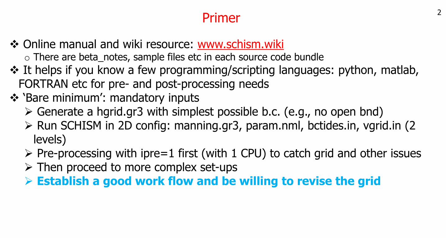
• /sciclone/home10/yinglong/vims20/schism_verification_tests/Test_CORIE/TMP% ls -L *.gr3 *.ll *.icalbedo.gr3 diffmax.gr3 drag.gr3 hgrid.gr3 SAL_nudge.gr3 TEM_nudge.gr3 windrot_geo2proj.gr3centers.gr3 diffmin.gr3 estuary.gr3 hgrid.ll sidecenters.gr3 watertype.gr3

• /sciclone/home10/yinglong/vims20/schism_verification_tests/Test_CORIE/TMP% ls -L *.in *.nmlbctides.in param.nml vgrid.in

• /sciclone/home10/yinglong/vims20/schism_verification_tests/Test_CORIE/TMP% ls -L *.th*flux.th TEM_1.th <- ASCII

• /sciclone/home10/yinglong/vims20/schism_verification_tests/Test_CORIE/TMP% ls -L *.nchotstart.nc SAL_nu.nc TEM_nu.nc

• /sciclone/home10/yinglong/vims20/schism_verification_tests/Test_CORIE/TMP% ls -Lalbedo.gr3 CORIE_TMP.o3660379 drag.gr3 fort.11 hotstart.nc postpros.pl run_bora show_schism_nc.m tmp.xyuv watertype.gr3bctides.in coriolis.out err2.out fort.17 mirror.out pschism_WHIRLWIND_Intel_VL run_whirlwind_openmpi sidecenters.gr3 total.dat windrot_geo2proj.gr3 bnd.xy date.in estuary.gr3 fort.33 SAL_nudge.gr3 TEM_1.th total_TR.datcenters.gr3 diffmax.gr3 flux.dat hgrid.gr3 outputs/ read.in SAL_nu.nc TEM_nudge.gr3 tvd.propCORIE_TMP.e3660379 diffmin.gr3 flux.th hgrid.ll param.nml README sflux/ TEM_nu.nc vgrid.in

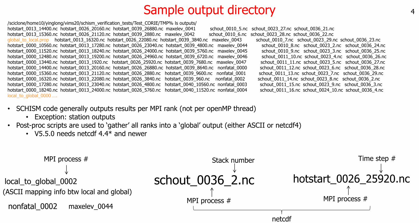
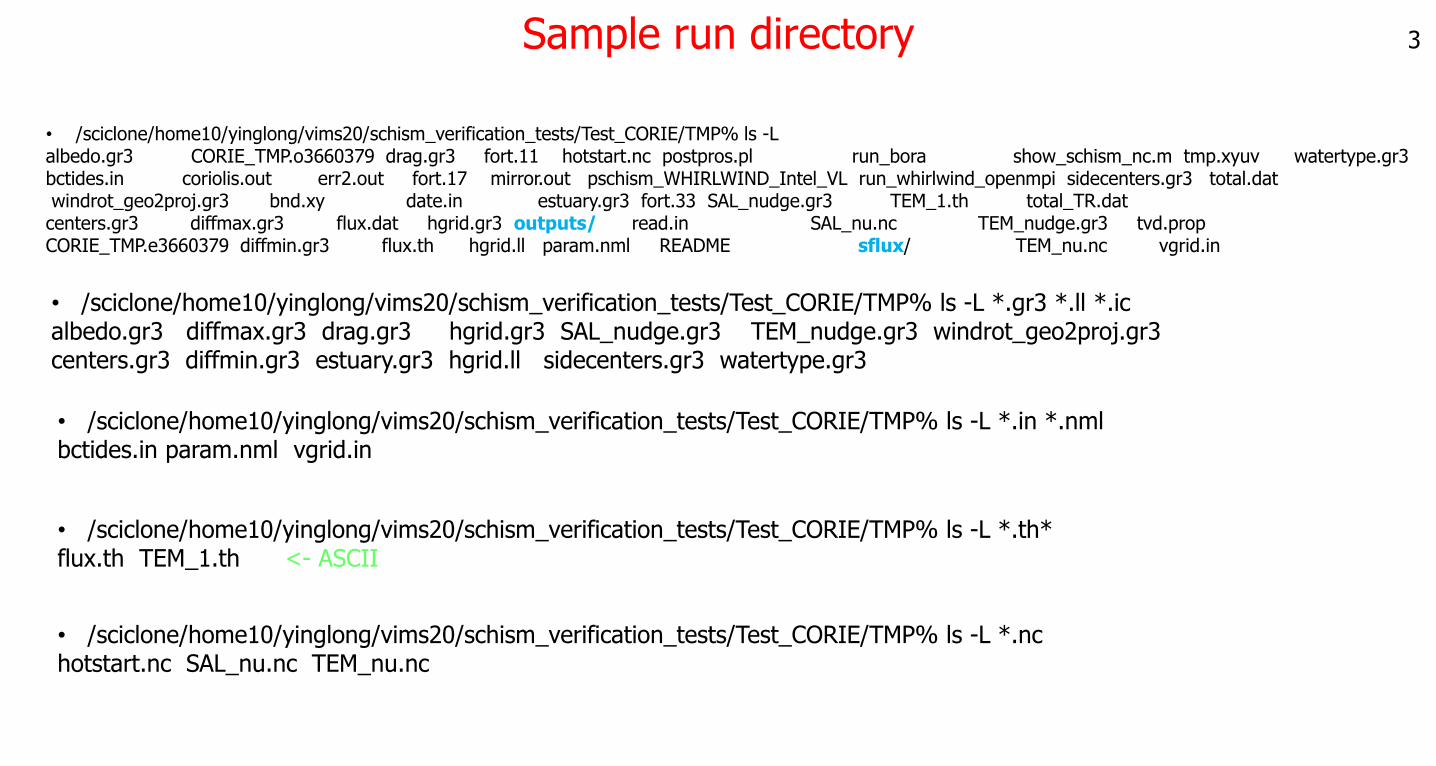
Sample output directory/sciclone/home10/yinglong/vims20/schism_verification_tests/Test_CORIE/TMP% ls outputs/hotstart_0013_14400.nc hotstart_0026_20160.nc hotstart_0039_26880.nc maxelev_0041 schout_0010_5.nc schout_0023_27.nc schout_0036_21.nchotstart_0013_15360.nc hotstart_0026_21120.nc hotstart_0039_2880.nc maxelev_0042 schout_0010_6.nc schout_0023_28.nc schout_0036_22.ncglobal_to_local.prop hotstart_0013_16320.nc hotstart_0026_22080.nc hotstart_0039_3840.nc maxelev_0043 schout_0010_7.nc schout_0023_29.nc schout_0036_23.nchotstart_0000_10560.nc hotstart_0013_17280.nc hotstart_0026_23040.nc hotstart_0039_4800.nc maxelev_0044 schout_0010_8.nc schout_0023_2.nc schout_0036_24.nchotstart_0000_11520.nc hotstart_0013_18240.nc hotstart_0026_24000.nc hotstart_0039_5760.nc maxelev_0045 schout_0010_9.nc schout_0023_3.nc schout_0036_25.nchotstart_0000_12480.nc hotstart_0013_19200.nc hotstart_0026_24960.nc hotstart_0039_6720.nc maxelev_0046 schout_0011_10.nc schout_0023_4.nc schout_0036_26.nchotstart_0000_13440.nc hotstart_0013_1920.nc hotstart_0026_25920.nc hotstart_0039_7680.nc maxelev_0047 schout_0011_11.nc schout_0023_5.nc schout_0036_27.nchotstart_0000_14400.nc hotstart_0013_20160.nc hotstart_0026_26880.nc hotstart_0039_8640.nc nonfatal_0000 schout_0011_12.nc schout_0023_6.nc schout_0036_28.nchotstart_0000_15360.nc hotstart_0013_21120.nc hotstart_0026_2880.nc hotstart_0039_9600.nc nonfatal_0001 schout_0011_13.nc schout_0023_7.nc schout_0036_29.nchotstart_0000_16320.nc hotstart_0013_22080.nc hotstart_0026_3840.nc hotstart_0039_960.nc nonfatal_0002 schout_0011_14.nc schout_0023_8.nc schout_0036_2.nchotstart_0000_17280.nc hotstart_0013_23040.nc hotstart_0026_4800.nc hotstart_0040_10560.nc nonfatal_0003 schout_0011_15.nc schout_0023_9.nc schout_0036_3.nchotstart_0000_18240.nc hotstart_0013_24000.nc hotstart_0026_5760.nc hotstart_0040_11520.nc nonfatal_0004 schout_0011_16.nc schout_0024_10.nc schout_0036_4.nclocal_to_global_0000 ….

schout_0036_2.nc

MPI process #

Stack number

hotstart_0026_25920.nc

MPI process #

Time step #

4

local_to_global_0002

MPI process #

• SCHISM code generally outputs results per MPI rank (not per openMP thread)• Exception: station outputs

• Post-proc scripts are used to ‘gather’ all ranks into a ‘global’ output (either ASCII or netcdf4)• V5.5.0 needs netcdf 4.4* and newer

(ASCII mapping info btw local and global)

netcdf

nonfatal_0002 maxelev_0044

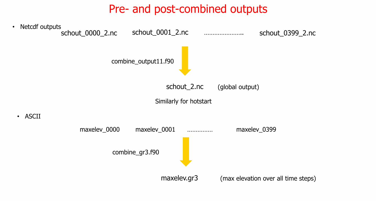
Pre- and post-combined outputs

schout_2.nc

schout_0001_2.nc schout_0399_2.nc…………………..

combine_output11.f90

schout_0000_2.nc

(global output)

Similarly for hotstart

maxelev_0000 maxelev_0001 …………… maxelev_0399

• Netcdf outputs

• ASCII

maxelev.gr3

combine_gr3.f90

(max elevation over all time steps)

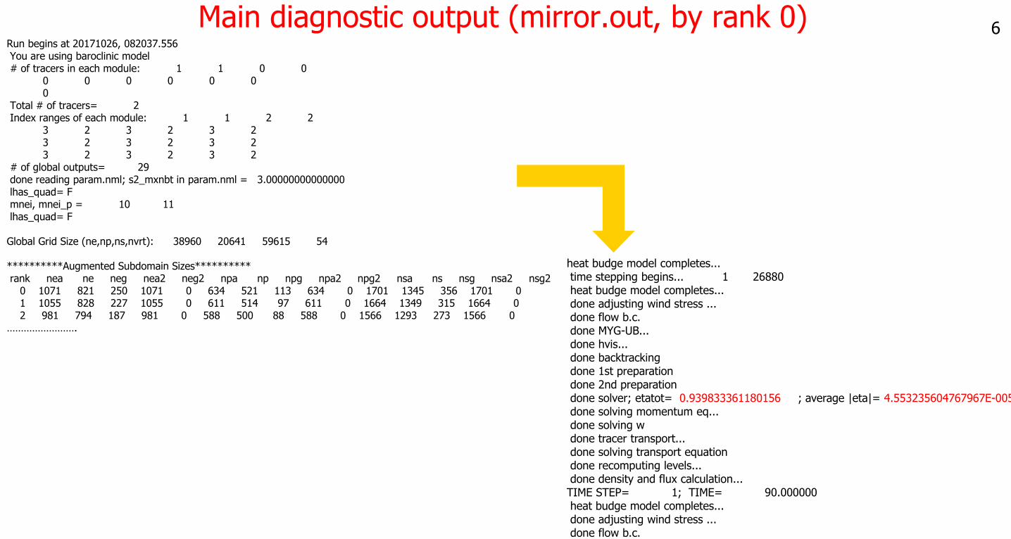
Main diagnostic output (mirror.out, by rank 0)Run begins at 20171026, 082037.556You are using baroclinic model# of tracers in each module: 1 1 0 0

0 0 0 0 0 00

Total # of tracers= 2Index ranges of each module: 1 1 2 2

3 2 3 2 3 23 2 3 2 3 23 2 3 2 3 2

# of global outputs= 29done reading param.nml; s2_mxnbt in param.nml = 3.00000000000000lhas_quad= Fmnei, mnei_p = 10 11lhas_quad= F

Global Grid Size (ne,np,ns,nvrt): 38960 20641 59615 54

**********Augmented Subdomain Sizes**********rank nea ne neg nea2 neg2 npa np npg npa2 npg2 nsa ns nsg nsa2 nsg2

0 1071 821 250 1071 0 634 521 113 634 0 1701 1345 356 1701 01 1055 828 227 1055 0 611 514 97 611 0 1664 1349 315 1664 02 981 794 187 981 0 588 500 88 588 0 1566 1293 273 1566 0

…………………….

heat budge model completes...time stepping begins... 1 26880heat budge model completes...done adjusting wind stress ...done flow b.c.done MYG-UB...done hvis...done backtrackingdone 1st preparationdone 2nd preparationdone solver; etatot= 0.939833361180156 ; average |eta|= 4.553235604767967E-005done solving momentum eq...done solving wdone tracer transport...done solving transport equationdone recomputing levels...done density and flux calculation...TIME STEP= 1; TIME= 90.000000heat budge model completes...done adjusting wind stress ...done flow b.c.

6

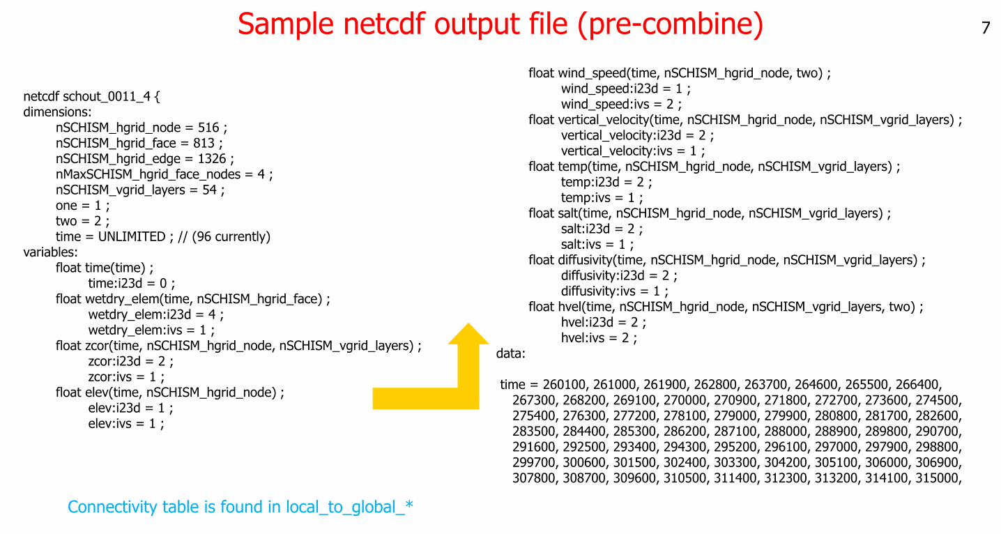
Sample netcdf output file (pre-combine)

netcdf schout_0011_4 {dimensions:

nSCHISM_hgrid_node = 516 ;nSCHISM_hgrid_face = 813 ;nSCHISM_hgrid_edge = 1326 ;nMaxSCHISM_hgrid_face_nodes = 4 ;nSCHISM_vgrid_layers = 54 ;one = 1 ;two = 2 ;time = UNLIMITED ; // (96 currently)

variables:float time(time) ;

time:i23d = 0 ;float wetdry_elem(time, nSCHISM_hgrid_face) ;

wetdry_elem:i23d = 4 ;wetdry_elem:ivs = 1 ;

float zcor(time, nSCHISM_hgrid_node, nSCHISM_vgrid_layers) ;zcor:i23d = 2 ;zcor:ivs = 1 ;

float elev(time, nSCHISM_hgrid_node) ;elev:i23d = 1 ;elev:ivs = 1 ;

float wind_speed(time, nSCHISM_hgrid_node, two) ;wind_speed:i23d = 1 ;wind_speed:ivs = 2 ;

float vertical_velocity(time, nSCHISM_hgrid_node, nSCHISM_vgrid_layers) ;vertical_velocity:i23d = 2 ;vertical_velocity:ivs = 1 ;

float temp(time, nSCHISM_hgrid_node, nSCHISM_vgrid_layers) ;temp:i23d = 2 ;temp:ivs = 1 ;

float salt(time, nSCHISM_hgrid_node, nSCHISM_vgrid_layers) ;salt:i23d = 2 ;salt:ivs = 1 ;

float diffusivity(time, nSCHISM_hgrid_node, nSCHISM_vgrid_layers) ;diffusivity:i23d = 2 ;diffusivity:ivs = 1 ;

float hvel(time, nSCHISM_hgrid_node, nSCHISM_vgrid_layers, two) ;hvel:i23d = 2 ;hvel:ivs = 2 ;

data:

time = 260100, 261000, 261900, 262800, 263700, 264600, 265500, 266400,267300, 268200, 269100, 270000, 270900, 271800, 272700, 273600, 274500,275400, 276300, 277200, 278100, 279000, 279900, 280800, 281700, 282600,283500, 284400, 285300, 286200, 287100, 288000, 288900, 289800, 290700,291600, 292500, 293400, 294300, 295200, 296100, 297000, 297900, 298800,299700, 300600, 301500, 302400, 303300, 304200, 305100, 306000, 306900,307800, 308700, 309600, 310500, 311400, 312300, 313200, 314100, 315000,

Connectivity table is found in local_to_global_*

7

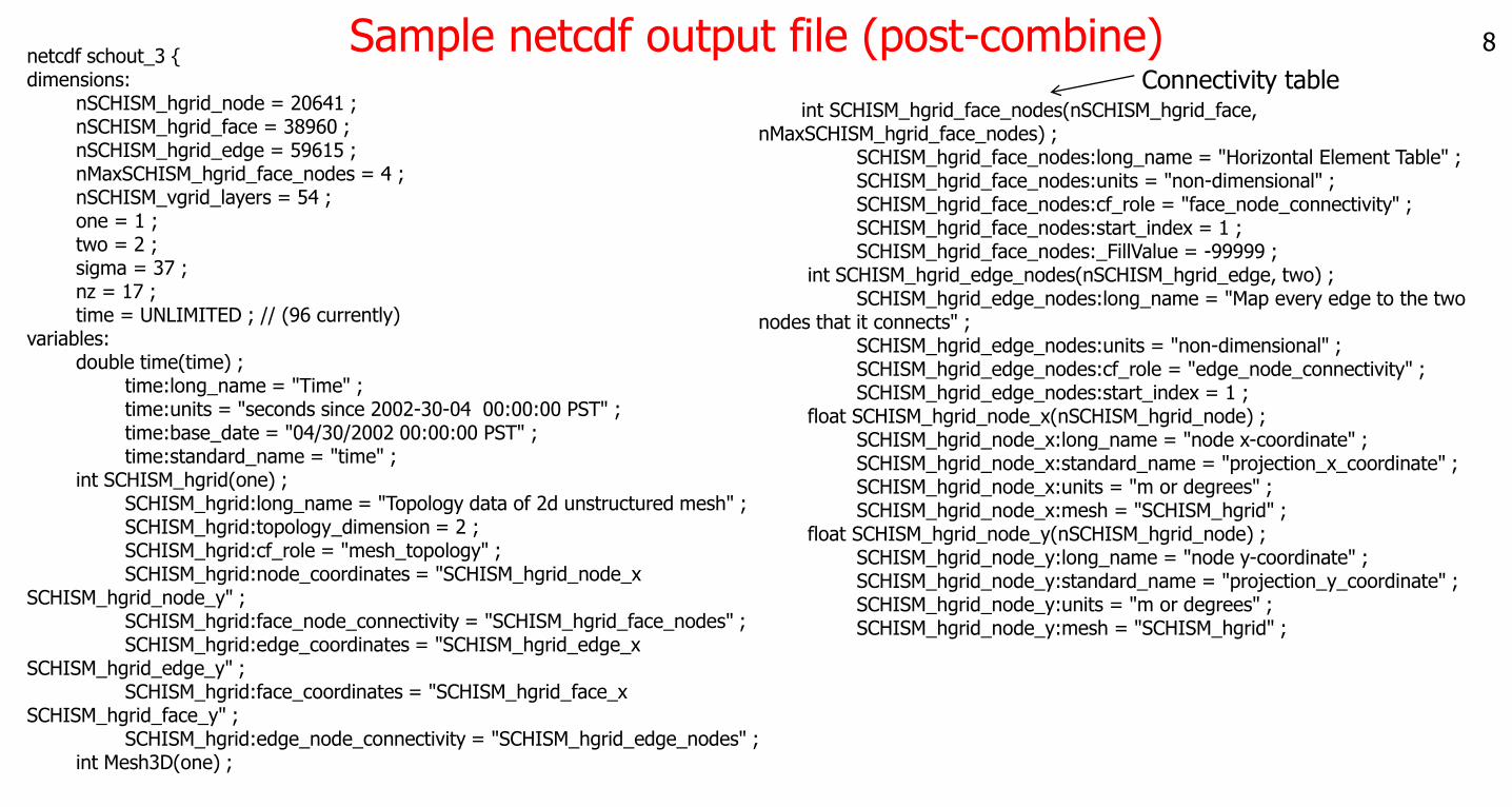
Sample netcdf output file (post-combine)netcdf schout_3 {dimensions:

nSCHISM_hgrid_node = 20641 ;nSCHISM_hgrid_face = 38960 ;nSCHISM_hgrid_edge = 59615 ;nMaxSCHISM_hgrid_face_nodes = 4 ;nSCHISM_vgrid_layers = 54 ;one = 1 ;two = 2 ;sigma = 37 ;nz = 17 ;time = UNLIMITED ; // (96 currently)

variables:double time(time) ;

time:long_name = "Time" ;time:units = "seconds since 2002-30-04 00:00:00 PST" ;time:base_date = "04/30/2002 00:00:00 PST" ;time:standard_name = "time" ;

int SCHISM_hgrid(one) ;SCHISM_hgrid:long_name = "Topology data of 2d unstructured mesh" ;SCHISM_hgrid:topology_dimension = 2 ;SCHISM_hgrid:cf_role = "mesh_topology" ;SCHISM_hgrid:node_coordinates = "SCHISM_hgrid_node_x

SCHISM_hgrid_node_y" ;SCHISM_hgrid:face_node_connectivity = "SCHISM_hgrid_face_nodes" ;SCHISM_hgrid:edge_coordinates = "SCHISM_hgrid_edge_x

SCHISM_hgrid_edge_y" ;SCHISM_hgrid:face_coordinates = "SCHISM_hgrid_face_x

SCHISM_hgrid_face_y" ;SCHISM_hgrid:edge_node_connectivity = "SCHISM_hgrid_edge_nodes" ;

int Mesh3D(one) ;

int SCHISM_hgrid_face_nodes(nSCHISM_hgrid_face, nMaxSCHISM_hgrid_face_nodes) ;

SCHISM_hgrid_face_nodes:long_name = "Horizontal Element Table" ;SCHISM_hgrid_face_nodes:units = "non-dimensional" ;SCHISM_hgrid_face_nodes:cf_role = "face_node_connectivity" ;SCHISM_hgrid_face_nodes:start_index = 1 ;SCHISM_hgrid_face_nodes:_FillValue = -99999 ;

int SCHISM_hgrid_edge_nodes(nSCHISM_hgrid_edge, two) ;SCHISM_hgrid_edge_nodes:long_name = "Map every edge to the two

nodes that it connects" ;SCHISM_hgrid_edge_nodes:units = "non-dimensional" ;SCHISM_hgrid_edge_nodes:cf_role = "edge_node_connectivity" ;SCHISM_hgrid_edge_nodes:start_index = 1 ;

float SCHISM_hgrid_node_x(nSCHISM_hgrid_node) ;SCHISM_hgrid_node_x:long_name = "node x-coordinate" ;SCHISM_hgrid_node_x:standard_name = "projection_x_coordinate" ;SCHISM_hgrid_node_x:units = "m or degrees" ;SCHISM_hgrid_node_x:mesh = "SCHISM_hgrid" ;

float SCHISM_hgrid_node_y(nSCHISM_hgrid_node) ;SCHISM_hgrid_node_y:long_name = "node y-coordinate" ;SCHISM_hgrid_node_y:standard_name = "projection_y_coordinate" ;SCHISM_hgrid_node_y:units = "m or degrees" ;SCHISM_hgrid_node_y:mesh = "SCHISM_hgrid" ;

Connectivity table

8

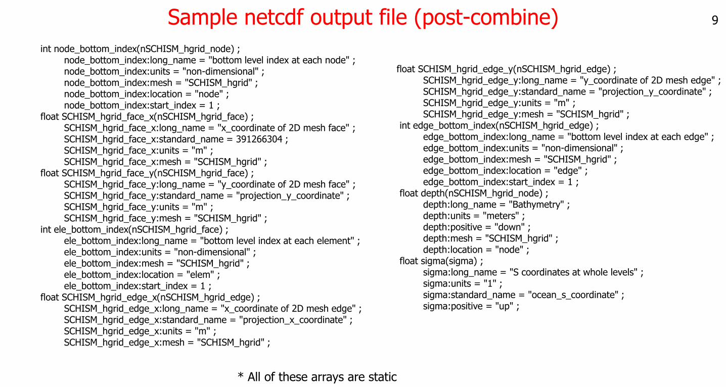
Sample netcdf output file (post-combine)

int node_bottom_index(nSCHISM_hgrid_node) ;node_bottom_index:long_name = "bottom level index at each node" ;node_bottom_index:units = "non-dimensional" ;node_bottom_index:mesh = "SCHISM_hgrid" ;node_bottom_index:location = "node" ;node_bottom_index:start_index = 1 ;

float SCHISM_hgrid_face_x(nSCHISM_hgrid_face) ;SCHISM_hgrid_face_x:long_name = "x_coordinate of 2D mesh face" ;SCHISM_hgrid_face_x:standard_name = 391266304 ;SCHISM_hgrid_face_x:units = "m" ;SCHISM_hgrid_face_x:mesh = "SCHISM_hgrid" ;

float SCHISM_hgrid_face_y(nSCHISM_hgrid_face) ;SCHISM_hgrid_face_y:long_name = "y_coordinate of 2D mesh face" ;SCHISM_hgrid_face_y:standard_name = "projection_y_coordinate" ;SCHISM_hgrid_face_y:units = "m" ;SCHISM_hgrid_face_y:mesh = "SCHISM_hgrid" ;

int ele_bottom_index(nSCHISM_hgrid_face) ;ele_bottom_index:long_name = "bottom level index at each element" ;ele_bottom_index:units = "non-dimensional" ;ele_bottom_index:mesh = "SCHISM_hgrid" ;ele_bottom_index:location = "elem" ;ele_bottom_index:start_index = 1 ;

float SCHISM_hgrid_edge_x(nSCHISM_hgrid_edge) ;SCHISM_hgrid_edge_x:long_name = "x_coordinate of 2D mesh edge" ;SCHISM_hgrid_edge_x:standard_name = "projection_x_coordinate" ;SCHISM_hgrid_edge_x:units = "m" ;SCHISM_hgrid_edge_x:mesh = "SCHISM_hgrid" ;

float SCHISM_hgrid_edge_y(nSCHISM_hgrid_edge) ;SCHISM_hgrid_edge_y:long_name = "y_coordinate of 2D mesh edge" ;SCHISM_hgrid_edge_y:standard_name = "projection_y_coordinate" ;SCHISM_hgrid_edge_y:units = "m" ;SCHISM_hgrid_edge_y:mesh = "SCHISM_hgrid" ;

int edge_bottom_index(nSCHISM_hgrid_edge) ;edge_bottom_index:long_name = "bottom level index at each edge" ;edge_bottom_index:units = "non-dimensional" ;edge_bottom_index:mesh = "SCHISM_hgrid" ;edge_bottom_index:location = "edge" ;edge_bottom_index:start_index = 1 ;

float depth(nSCHISM_hgrid_node) ;depth:long_name = "Bathymetry" ;depth:units = "meters" ;depth:positive = "down" ;depth:mesh = "SCHISM_hgrid" ;depth:location = "node" ;

float sigma(sigma) ;sigma:long_name = "S coordinates at whole levels" ;sigma:units = "1" ;sigma:standard_name = "ocean_s_coordinate" ;sigma:positive = "up" ;

9

* All of these arrays are static

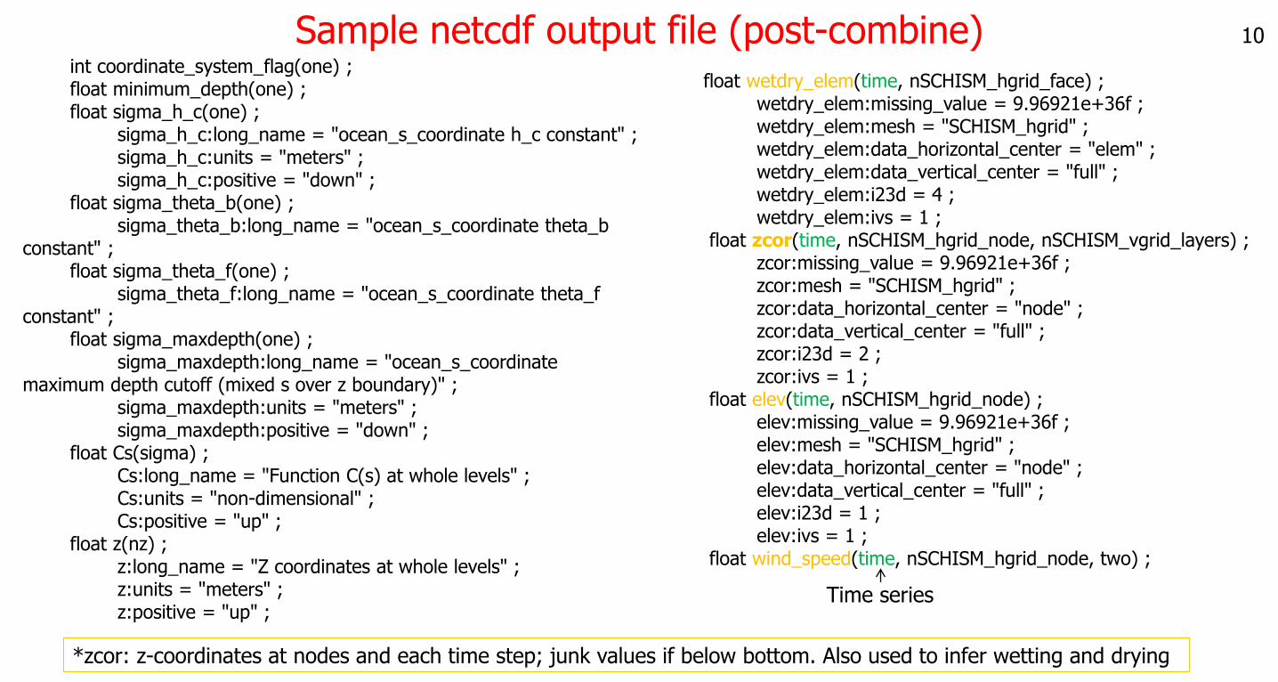
Sample netcdf output file (post-combine)int coordinate_system_flag(one) ;float minimum_depth(one) ;float sigma_h_c(one) ;

sigma_h_c:long_name = "ocean_s_coordinate h_c constant" ;sigma_h_c:units = "meters" ;sigma_h_c:positive = "down" ;

float sigma_theta_b(one) ;sigma_theta_b:long_name = "ocean_s_coordinate theta_b

constant" ;float sigma_theta_f(one) ;

sigma_theta_f:long_name = "ocean_s_coordinate theta_fconstant" ;

float sigma_maxdepth(one) ;sigma_maxdepth:long_name = "ocean_s_coordinate

maximum depth cutoff (mixed s over z boundary)" ;sigma_maxdepth:units = "meters" ;sigma_maxdepth:positive = "down" ;

float Cs(sigma) ;Cs:long_name = "Function C(s) at whole levels" ;Cs:units = "non-dimensional" ;Cs:positive = "up" ;

float z(nz) ;z:long_name = "Z coordinates at whole levels" ;z:units = "meters" ;z:positive = "up" ;

float wetdry_elem(time, nSCHISM_hgrid_face) ;wetdry_elem:missing_value = 9.96921e+36f ;wetdry_elem:mesh = "SCHISM_hgrid" ;wetdry_elem:data_horizontal_center = "elem" ;wetdry_elem:data_vertical_center = "full" ;wetdry_elem:i23d = 4 ;wetdry_elem:ivs = 1 ;

float zcor(time, nSCHISM_hgrid_node, nSCHISM_vgrid_layers) ;zcor:missing_value = 9.96921e+36f ;zcor:mesh = "SCHISM_hgrid" ;zcor:data_horizontal_center = "node" ;zcor:data_vertical_center = "full" ;zcor:i23d = 2 ;zcor:ivs = 1 ;

float elev(time, nSCHISM_hgrid_node) ;elev:missing_value = 9.96921e+36f ;elev:mesh = "SCHISM_hgrid" ;elev:data_horizontal_center = "node" ;elev:data_vertical_center = "full" ;elev:i23d = 1 ;elev:ivs = 1 ;

float wind_speed(time, nSCHISM_hgrid_node, two) ;

Time series

10

*zcor: z-coordinates at nodes and each time step; junk values if below bottom. Also used to infer wetting and drying

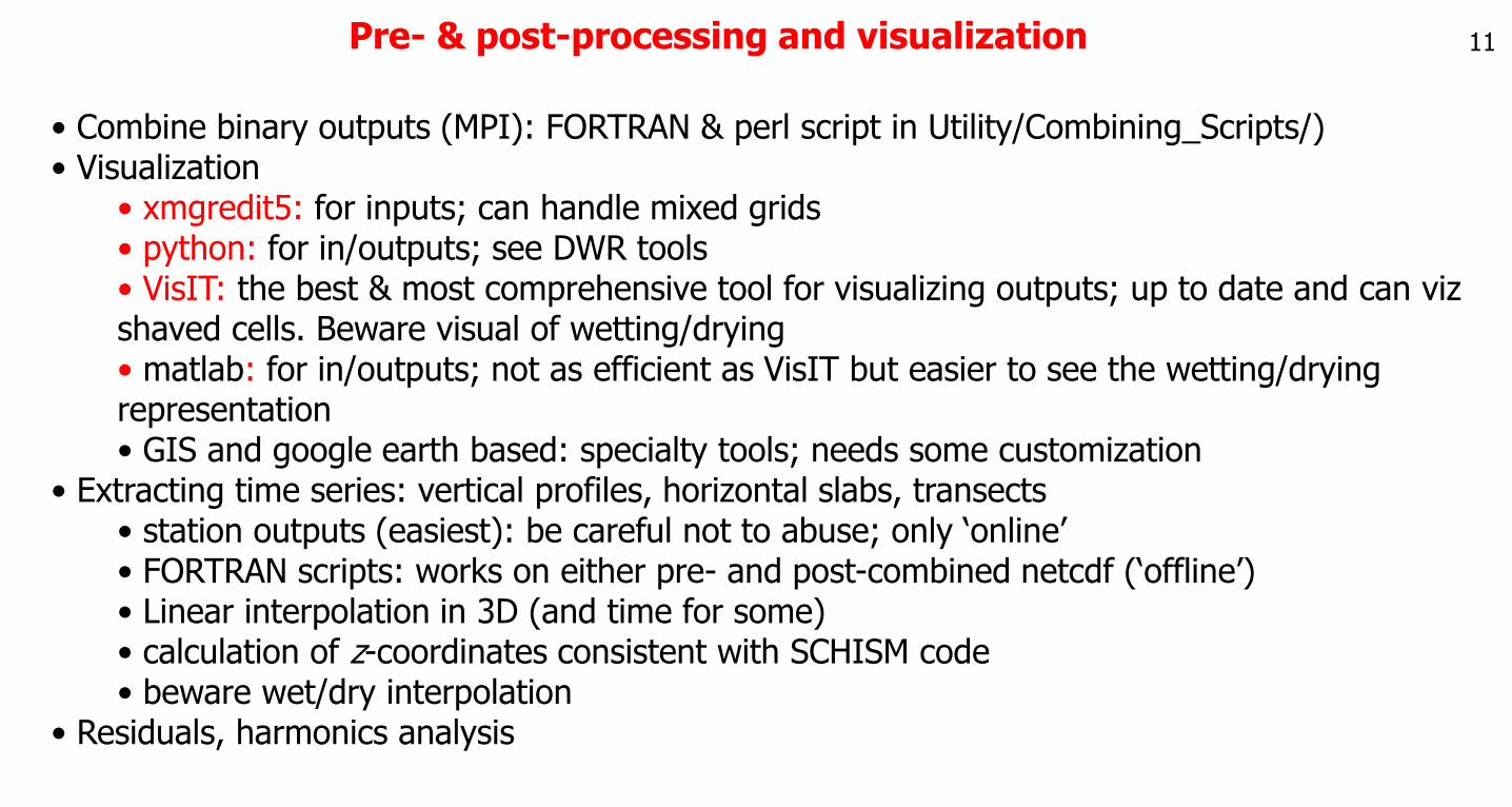
11Pre- & post-processing and visualization

• Combine binary outputs (MPI): FORTRAN & perl script in Utility/Combining_Scripts/)• Visualization

• xmgredit5: for inputs; can handle mixed grids• python: for in/outputs; see DWR tools• VisIT: the best & most comprehensive tool for visualizing outputs; up to date and can vizshaved cells. Beware visual of wetting/drying• matlab: for in/outputs; not as efficient as VisIT but easier to see the wetting/drying representation• GIS and google earth based: specialty tools; needs some customization

• Extracting time series: vertical profiles, horizontal slabs, transects• station outputs (easiest): be careful not to abuse; only ‘online’• FORTRAN scripts: works on either pre- and post-combined netcdf (‘offline’)• Linear interpolation in 3D (and time for some)• calculation of z-coordinates consistent with SCHISM code• beware wet/dry interpolation

• Residuals, harmonics analysis

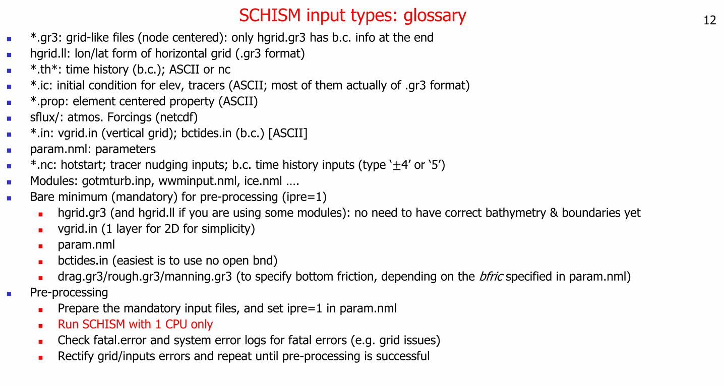
12SCHISM input types: glossary *.gr3: grid-like files (node centered): only hgrid.gr3 has b.c. info at the end

hgrid.ll: lon/lat form of horizontal grid (.gr3 format)

*.th*: time history (b.c.); ASCII or nc

*.ic: initial condition for elev, tracers (ASCII; most of them actually of .gr3 format)

*.prop: element centered property (ASCII)

sflux/: atmos. Forcings (netcdf)

*.in: vgrid.in (vertical grid); bctides.in (b.c.) [ASCII]

param.nml: parameters

*.nc: hotstart; tracer nudging inputs; b.c. time history inputs (type ‘±4’ or ‘5’)

Modules: gotmturb.inp, wwminput.nml, ice.nml ….

Bare minimum (mandatory) for pre-processing (ipre=1)

hgrid.gr3 (and hgrid.ll if you are using some modules): no need to have correct bathymetry & boundaries yet

vgrid.in (1 layer for 2D for simplicity)

param.nml

bctides.in (easiest is to use no open bnd)

drag.gr3/rough.gr3/manning.gr3 (to specify bottom friction, depending on the bfric specified in param.nml)

Pre-processing

Prepare the mandatory input files, and set ipre=1 in param.nml

Run SCHISM with 1 CPU only

Check fatal.error and system error logs for fatal errors (e.g. grid issues)

Rectify grid/inputs errors and repeat until pre-processing is successful

Details of model setup

13

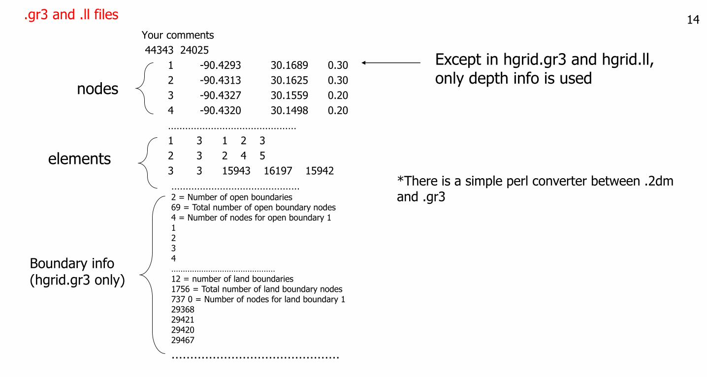
14.gr3 and .ll files

Your comments

44343 24025

1 -90.4293 30.1689 0.30

2 -90.4313 30.1625 0.30

3 -90.4327 30.1559 0.20

4 -90.4320 30.1498 0.20

………………………………………

1 3 1 2 3

2 3 2 4 5

3 3 15943 16197 15942

………………………………………

nodes

elements

Boundary info(hgrid.gr3 only)

2 = Number of open boundaries69 = Total number of open boundary nodes4 = Number of nodes for open boundary 11234………………………………………12 = number of land boundaries1756 = Total number of land boundary nodes737 0 = Number of nodes for land boundary 129368294212942029467

………………………………………

Except in hgrid.gr3 and hgrid.ll, only depth info is used

*There is a simple perl converter between .2dm and .gr3

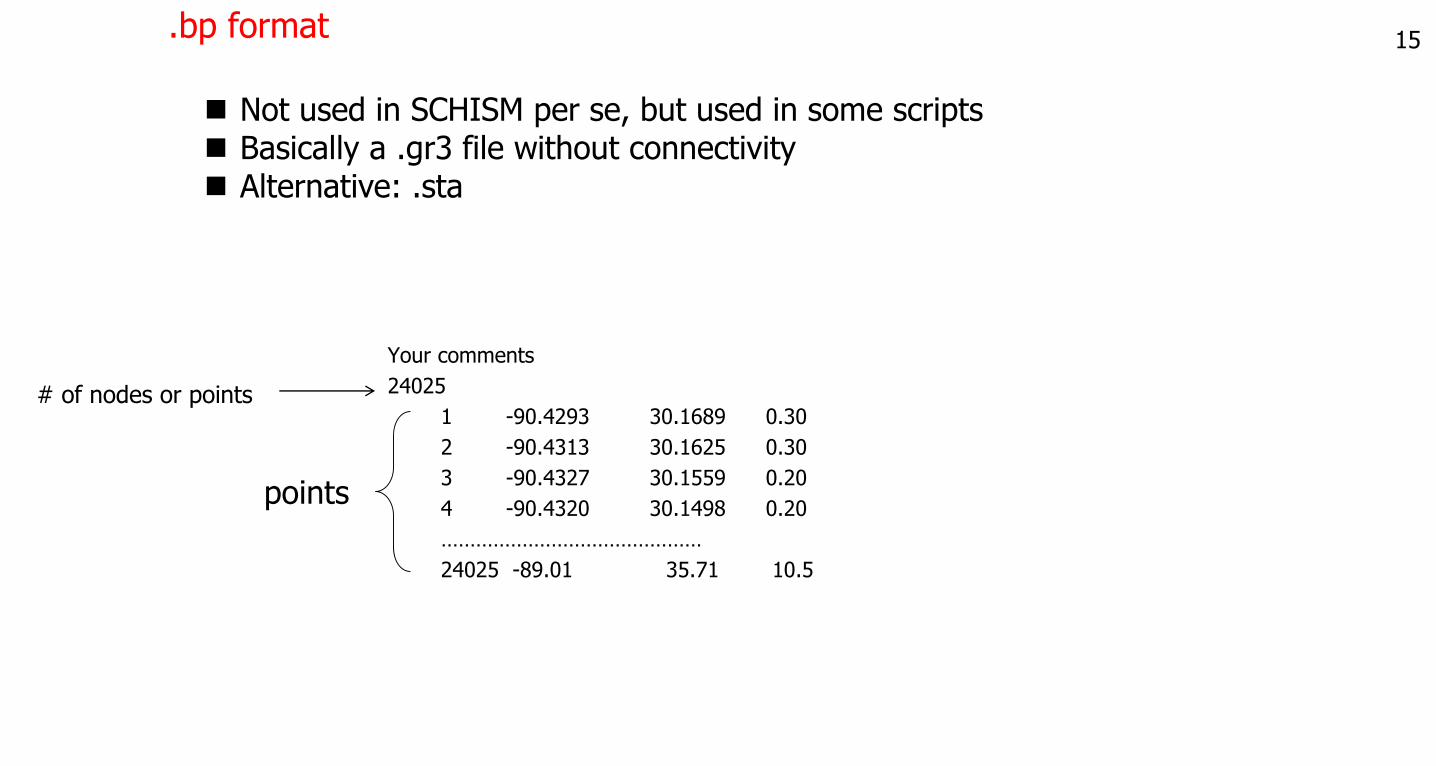
15.bp format

Your comments

24025

1 -90.4293 30.1689 0.30

2 -90.4313 30.1625 0.30

3 -90.4327 30.1559 0.20

4 -90.4320 30.1498 0.20

………………………………………

24025 -89.01 35.71 10.5

points

Not used in SCHISM per se, but used in some scripts Basically a .gr3 file without connectivity Alternative: .sta

# of nodes or points

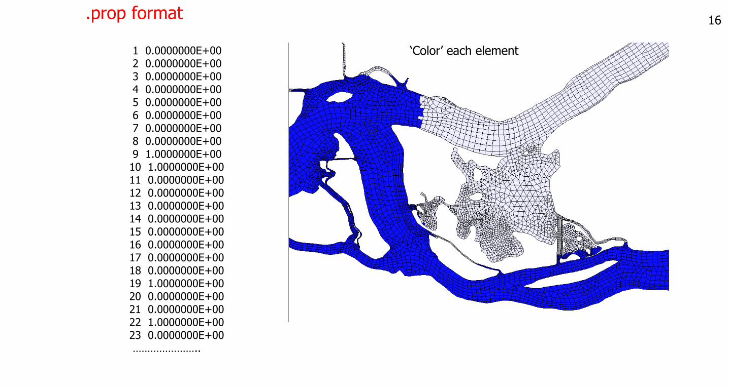
16.prop format

1 0.0000000E+002 0.0000000E+003 0.0000000E+004 0.0000000E+005 0.0000000E+006 0.0000000E+007 0.0000000E+008 0.0000000E+009 1.0000000E+0010 1.0000000E+0011 0.0000000E+0012 0.0000000E+0013 0.0000000E+0014 0.0000000E+0015 0.0000000E+0016 0.0000000E+0017 0.0000000E+0018 0.0000000E+0019 1.0000000E+0020 0.0000000E+0021 0.0000000E+0022 1.0000000E+0023 0.0000000E+00…………………..

‘Color’ each element

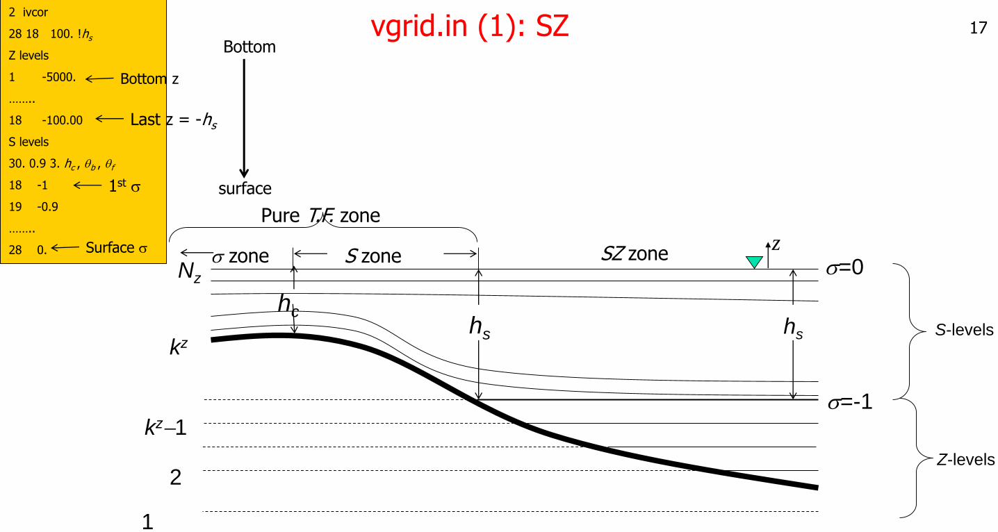
17vgrid.in (1): SZ2 ivcor

28 18 100. !hs

Z levels

1 -5000.

……..

18 -100.00

S levels

30. 0.9 3. hc , qb , qf

18 -1

19 -0.9

……..

28 0. s zone

1

hs

2

Nz

kz

s=0

s=-1

S-levels

Z-levels

kz-1

zS zone SZ zone

Pure T.F. zone

hs

hc

Bottom z

Last z = -hs

1st s

Surface s

Bottom

surface

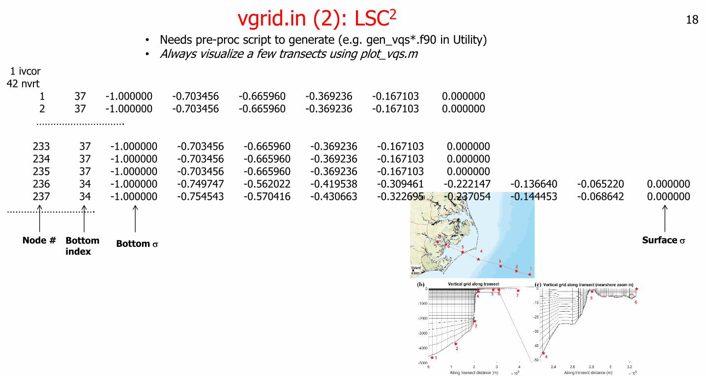
18vgrid.in (2): LSC2

1 ivcor42 nvrt

1 37 -1.000000 -0.703456 -0.665960 -0.369236 -0.167103 0.0000002 37 -1.000000 -0.703456 -0.665960 -0.369236 -0.167103 0.000000

………………………….

233 37 -1.000000 -0.703456 -0.665960 -0.369236 -0.167103 0.000000234 37 -1.000000 -0.703456 -0.665960 -0.369236 -0.167103 0.000000235 37 -1.000000 -0.703456 -0.665960 -0.369236 -0.167103 0.000000236 34 -1.000000 -0.749747 -0.562022 -0.419538 -0.309461 -0.222147 -0.136640 -0.065220 0.000000237 34 -1.000000 -0.754543 -0.570416 -0.430663 -0.322695 -0.237054 -0.144453 -0.068642 0.000000

………………………….

Node # Bottom index

Bottom s Surface s

• Needs pre-proc script to generate (e.g. gen_vqs*.f90 in Utility)• Always visualize a few transects using plot_vqs.m

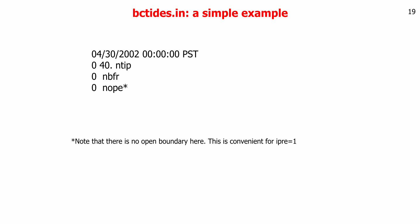
bctides.in: a simple example

04/30/2002 00:00:00 PST0 40. ntip0 nbfr0 nope*

*Note that there is no open boundary here. This is convenient for ipre=1

19

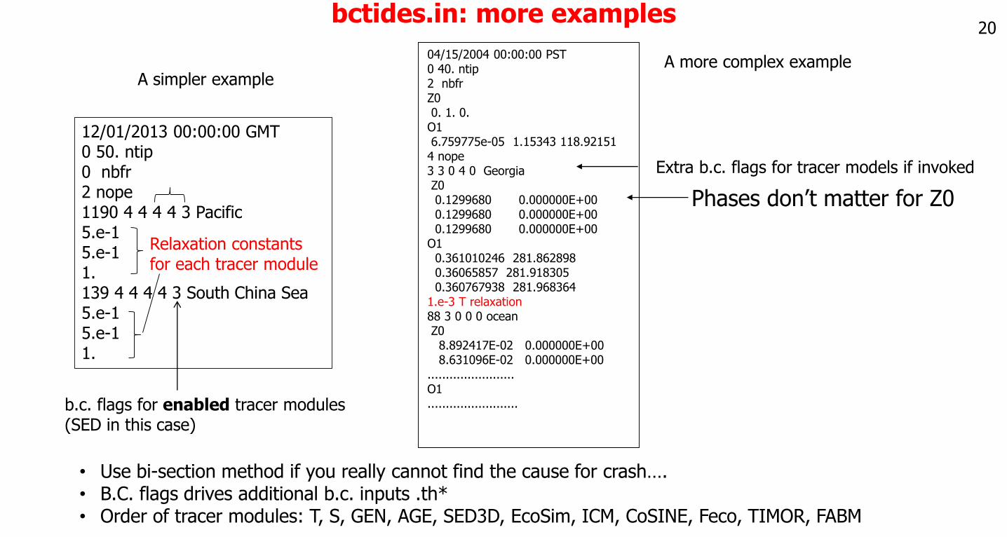
bctides.in: more examples

04/15/2004 00:00:00 PST0 40. ntip2 nbfrZ00. 1. 0.

O16.759775e-05 1.15343 118.92151

4 nope3 3 0 4 0 Georgia Z00.1299680 0.000000E+000.1299680 0.000000E+000.1299680 0.000000E+00

O10.361010246 281.8628980.36065857 281.9183050.360767938 281.968364

1.e-3 T relaxation88 3 0 0 0 oceanZ0

8.892417E-02 0.000000E+008.631096E-02 0.000000E+00

........................O1.........................

Phases don’t matter for Z0

Extra b.c. flags for tracer models if invoked

12/01/2013 00:00:00 GMT0 50. ntip0 nbfr2 nope1190 4 4 4 4 3 Pacific5.e-15.e-11.139 4 4 4 4 3 South China Sea5.e-15.e-11.

A simpler example

b.c. flags for enabled tracer modules (SED in this case)

• Use bi-section method if you really cannot find the cause for crash….• B.C. flags drives additional b.c. inputs .th*• Order of tracer modules: T, S, GEN, AGE, SED3D, EcoSim, ICM, CoSINE, Feco, TIMOR, FABM

20

A more complex example

Relaxation constants for each tracer module

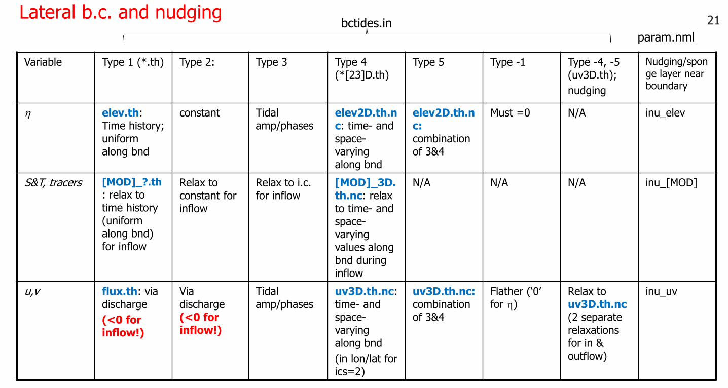
21Lateral b.c. and nudging

Variable Type 1 (*.th) Type 2: Type 3 Type 4 (*[23]D.th)

Type 5 Type -1 Type -4, -5 (uv3D.th);

nudging

Nudging/sponge layer near boundary

h elev.th: Time history; uniform along bnd

constant Tidal amp/phases

elev2D.th.nc: time- and space-varying along bnd

elev2D.th.nc: combination of 3&4

Must =0 N/A inu_elev

S&T, tracers [MOD]_?.th

: relax to time history (uniform along bnd) for inflow

Relax to constant for inflow

Relax to i.c. for inflow

[MOD]_3D.th.nc: relax to time- and space-varying values along bnd during inflow

N/A N/A N/A inu_[MOD]

u,v flux.th: via discharge

(<0 for inflow!)

Via discharge (<0 for inflow!)

Tidal amp/phases

uv3D.th.nc: time- and space-varying along bnd

(in lon/lat for ics=2)

uv3D.th.nc: combination of 3&4

Flather (‘0’ for h)

Relax to uv3D.th.nc(2 separate relaxations for in & outflow)

inu_uv

bctides.inparam.nml

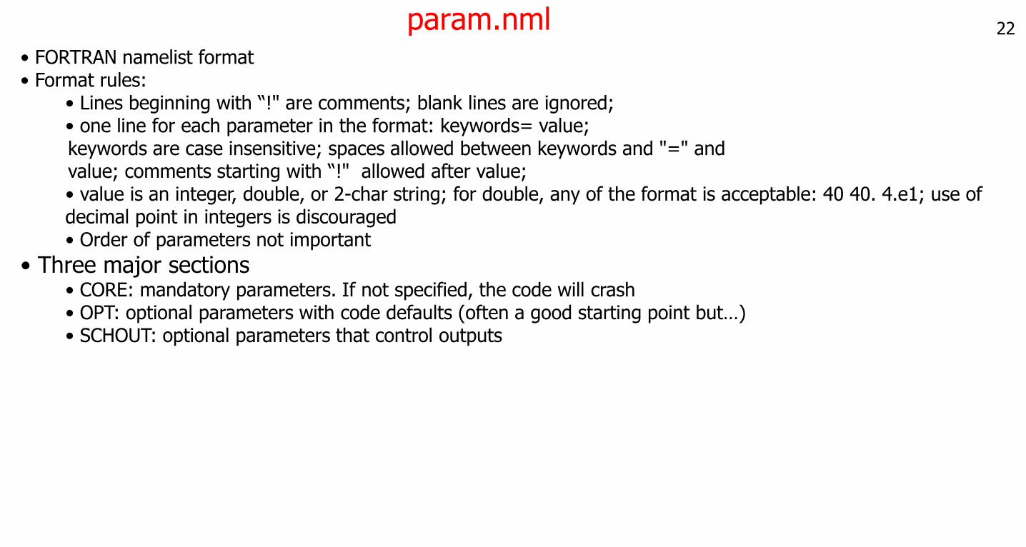
22param.nml• FORTRAN namelist format• Format rules:

• Lines beginning with “!" are comments; blank lines are ignored;• one line for each parameter in the format: keywords= value;keywords are case insensitive; spaces allowed between keywords and "=" and value; comments starting with “!" allowed after value;• value is an integer, double, or 2-char string; for double, any of the format is acceptable: 40 40. 4.e1; use of decimal point in integers is discouraged• Order of parameters not important

• Three major sections• CORE: mandatory parameters. If not specified, the code will crash• OPT: optional parameters with code defaults (often a good starting point but…)• SCHOUT: optional parameters that control outputs

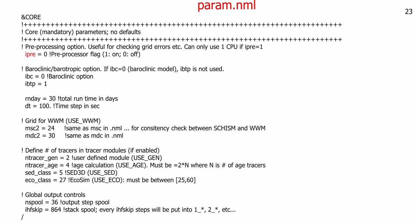
23param.nml

&CORE!+++++++++++++++++++++++++++++++++++++++++++++++++++++++++++++++++++++++! Core (mandatory) parameters; no defaults!+++++++++++++++++++++++++++++++++++++++++++++++++++++++++++++++++++++++! Pre-processing option. Useful for checking grid errors etc. Can only use 1 CPU if ipre=1 ipre = 0 !Pre-processor flag (1: on; 0: off)

! Baroclinic/barotropic option. If ibc=0 (baroclinic model), ibtp is not used.ibc = 0 !Baroclinic optionibtp = 1

rnday = 30 !total run time in daysdt = 100. !Time step in sec

! Grid for WWM (USE_WWM)msc2 = 24 !same as msc in .nml ... for consitency check between SCHISM and WWMmdc2 = 30 !same as mdc in .nml

! Define # of tracers in tracer modules (if enabled)ntracer_gen = 2 !user defined module (USE_GEN)ntracer_age = 4 !age calculation (USE_AGE). Must be =2*N where N is # of age tracerssed_class = 5 !SED3D (USE_SED)eco_class = 27 !EcoSim (USE_ECO): must be between [25,60]

! Global output controlsnspool = 36 !output step spoolihfskip = 864 !stack spool; every ihfskip steps will be put into 1_*, 2_*, etc...

/

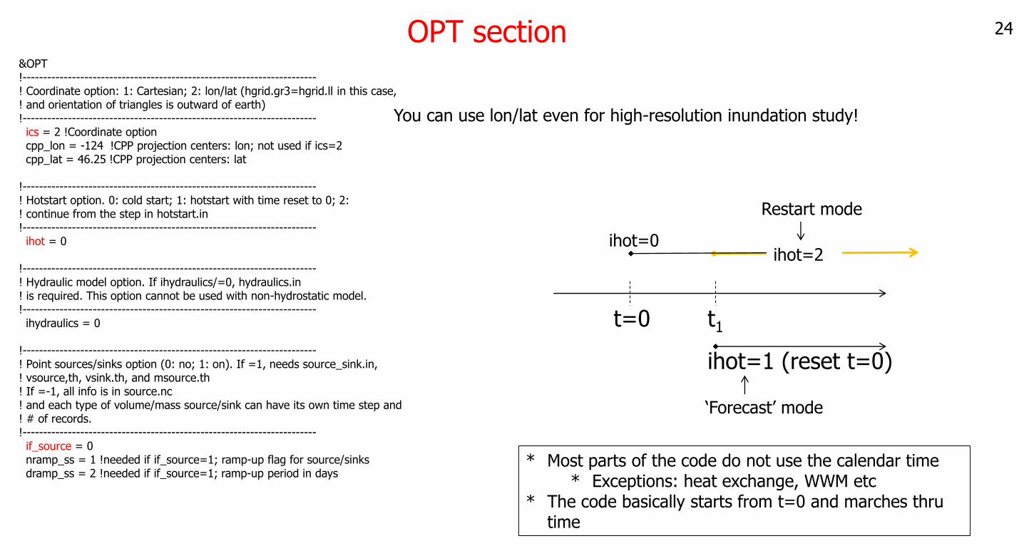
24OPT section

t=0 t1

ihot=1 (reset t=0)

You can use lon/lat even for high-resolution inundation study!

&OPT!-----------------------------------------------------------------------! Coordinate option: 1: Cartesian; 2: lon/lat (hgrid.gr3=hgrid.ll in this case,! and orientation of triangles is outward of earth) !-----------------------------------------------------------------------ics = 2 !Coordinate optioncpp_lon = -124 !CPP projection centers: lon; not used if ics=2cpp_lat = 46.25 !CPP projection centers: lat

!-----------------------------------------------------------------------! Hotstart option. 0: cold start; 1: hotstart with time reset to 0; 2:! continue from the step in hotstart.in!-----------------------------------------------------------------------ihot = 0

!-----------------------------------------------------------------------! Hydraulic model option. If ihydraulics/=0, hydraulics.in! is required. This option cannot be used with non-hydrostatic model.!-----------------------------------------------------------------------ihydraulics = 0

!-----------------------------------------------------------------------! Point sources/sinks option (0: no; 1: on). If =1, needs source_sink.in,! vsource,th, vsink.th, and msource.th! If =-1, all info is in source.nc! and each type of volume/mass source/sink can have its own time step and! # of records.!-----------------------------------------------------------------------if_source = 0nramp_ss = 1 !needed if if_source=1; ramp-up flag for source/sinksdramp_ss = 2 !needed if if_source=1; ramp-up period in days

Restart mode

‘Forecast’ mode

ihot=2ihot=0

* Most parts of the code do not use the calendar time* Exceptions: heat exchange, WWM etc

* The code basically starts from t=0 and marches thru time

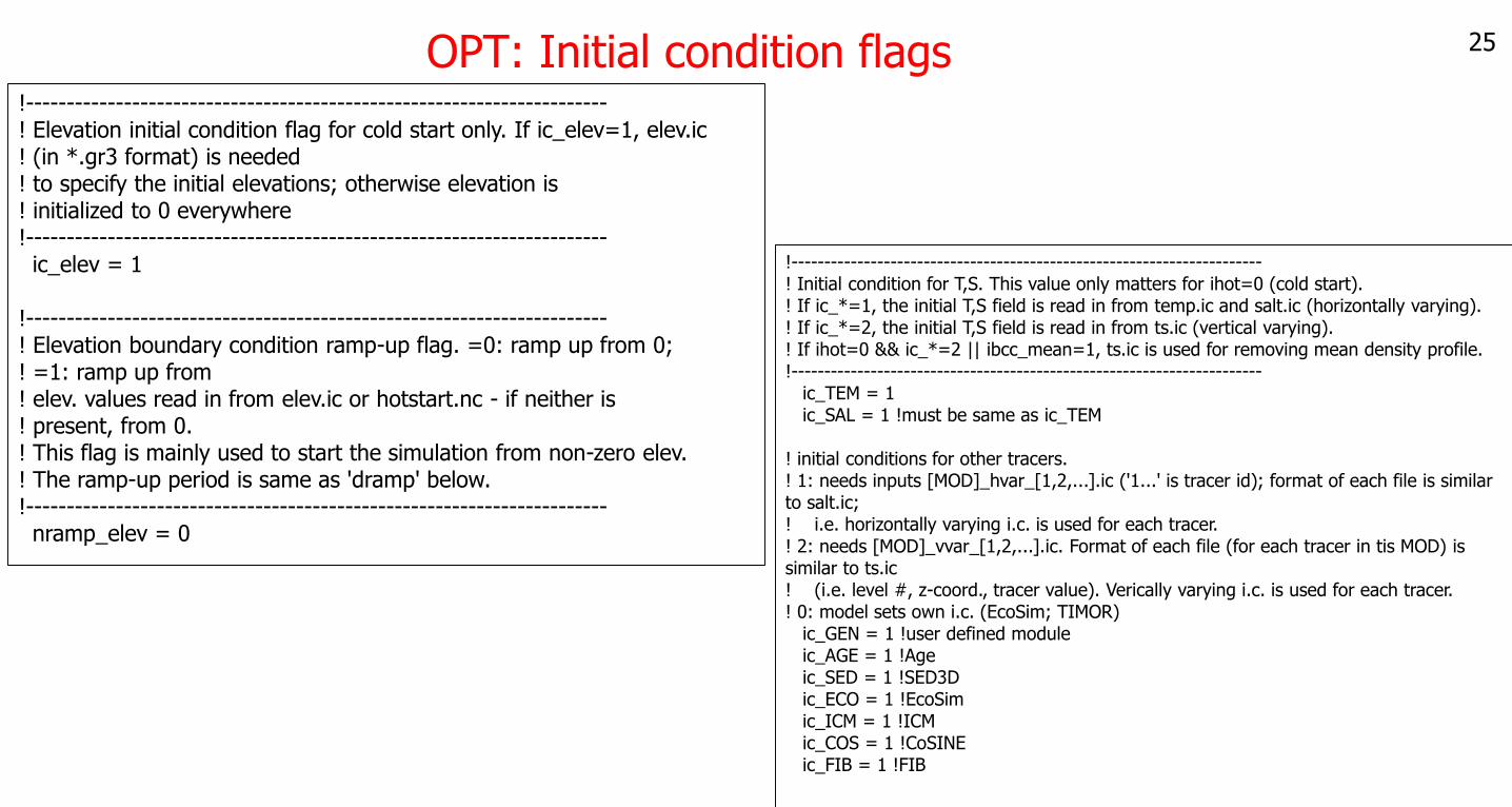
25OPT: Initial condition flags

!-----------------------------------------------------------------------! Initial condition for T,S. This value only matters for ihot=0 (cold start).! If ic_*=1, the initial T,S field is read in from temp.ic and salt.ic (horizontally varying).! If ic_*=2, the initial T,S field is read in from ts.ic (vertical varying).! If ihot=0 && ic_*=2 || ibcc_mean=1, ts.ic is used for removing mean density profile.!-----------------------------------------------------------------------

ic_TEM = 1ic_SAL = 1 !must be same as ic_TEM

! initial conditions for other tracers.! 1: needs inputs [MOD]_hvar_[1,2,...].ic ('1...' is tracer id); format of each file is similar to salt.ic;! i.e. horizontally varying i.c. is used for each tracer.! 2: needs [MOD]_vvar_[1,2,...].ic. Format of each file (for each tracer in tis MOD) is similar to ts.ic! (i.e. level #, z-coord., tracer value). Verically varying i.c. is used for each tracer.! 0: model sets own i.c. (EcoSim; TIMOR)

ic_GEN = 1 !user defined moduleic_AGE = 1 !Ageic_SED = 1 !SED3Dic_ECO = 1 !EcoSimic_ICM = 1 !ICMic_COS = 1 !CoSINEic_FIB = 1 !FIB

!-----------------------------------------------------------------------! Elevation initial condition flag for cold start only. If ic_elev=1, elev.ic! (in *.gr3 format) is needed! to specify the initial elevations; otherwise elevation is ! initialized to 0 everywhere!-----------------------------------------------------------------------ic_elev = 1

!-----------------------------------------------------------------------! Elevation boundary condition ramp-up flag. =0: ramp up from 0; ! =1: ramp up from! elev. values read in from elev.ic or hotstart.nc - if neither is ! present, from 0.! This flag is mainly used to start the simulation from non-zero elev.! The ramp-up period is same as 'dramp' below.!-----------------------------------------------------------------------nramp_elev = 0

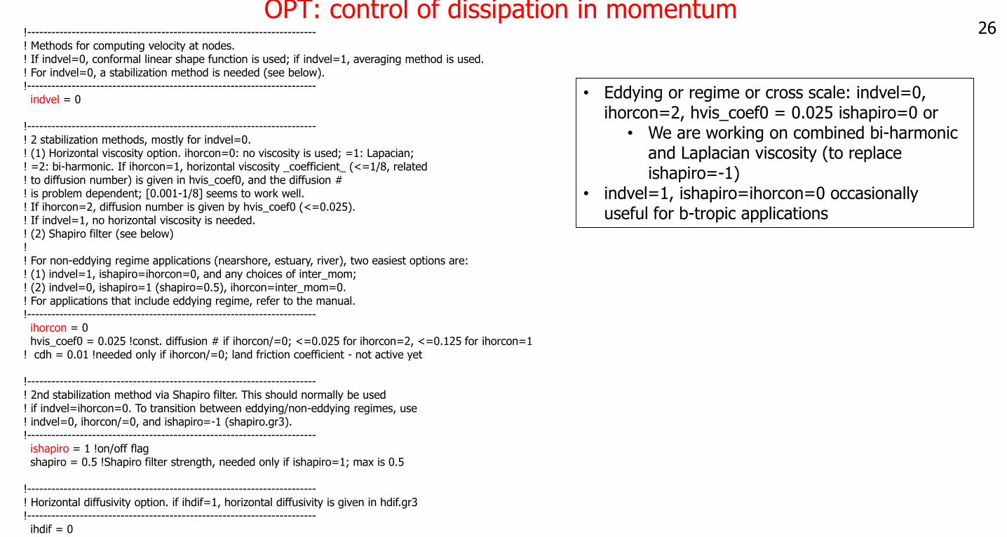
26OPT: control of dissipation in momentum

• Eddying or regime or cross scale: indvel=0, ihorcon=2, hvis_coef0 = 0.025 ishapiro=0 or

• We are working on combined bi-harmonic and Laplacian viscosity (to replace ishapiro=-1)

• indvel=1, ishapiro=ihorcon=0 occasionally useful for b-tropic applications

!-----------------------------------------------------------------------! Methods for computing velocity at nodes.! If indvel=0, conformal linear shape function is used; if indvel=1, averaging method is used.! For indvel=0, a stabilization method is needed (see below).!-----------------------------------------------------------------------indvel = 0

!-----------------------------------------------------------------------! 2 stabilization methods, mostly for indvel=0.! (1) Horizontal viscosity option. ihorcon=0: no viscosity is used; =1: Lapacian;! =2: bi-harmonic. If ihorcon=1, horizontal viscosity _coefficient_ (<=1/8, related! to diffusion number) is given in hvis_coef0, and the diffusion #! is problem dependent; [0.001-1/8] seems to work well.! If ihorcon=2, diffusion number is given by hvis_coef0 (<=0.025).! If indvel=1, no horizontal viscosity is needed.! (2) Shapiro filter (see below)!! For non-eddying regime applications (nearshore, estuary, river), two easiest options are:! (1) indvel=1, ishapiro=ihorcon=0, and any choices of inter_mom;! (2) indvel=0, ishapiro=1 (shapiro=0.5), ihorcon=inter_mom=0.! For applications that include eddying regime, refer to the manual.!-----------------------------------------------------------------------ihorcon = 0hvis_coef0 = 0.025 !const. diffusion # if ihorcon/=0; <=0.025 for ihorcon=2, <=0.125 for ihorcon=1

! cdh = 0.01 !needed only if ihorcon/=0; land friction coefficient - not active yet

!-----------------------------------------------------------------------! 2nd stabilization method via Shapiro filter. This should normally be used! if indvel=ihorcon=0. To transition between eddying/non-eddying regimes, use! indvel=0, ihorcon/=0, and ishapiro=-1 (shapiro.gr3).!-----------------------------------------------------------------------ishapiro = 1 !on/off flagshapiro = 0.5 !Shapiro filter strength, needed only if ishapiro=1; max is 0.5

!-----------------------------------------------------------------------! Horizontal diffusivity option. if ihdif=1, horizontal diffusivity is given in hdif.gr3!-----------------------------------------------------------------------ihdif = 0

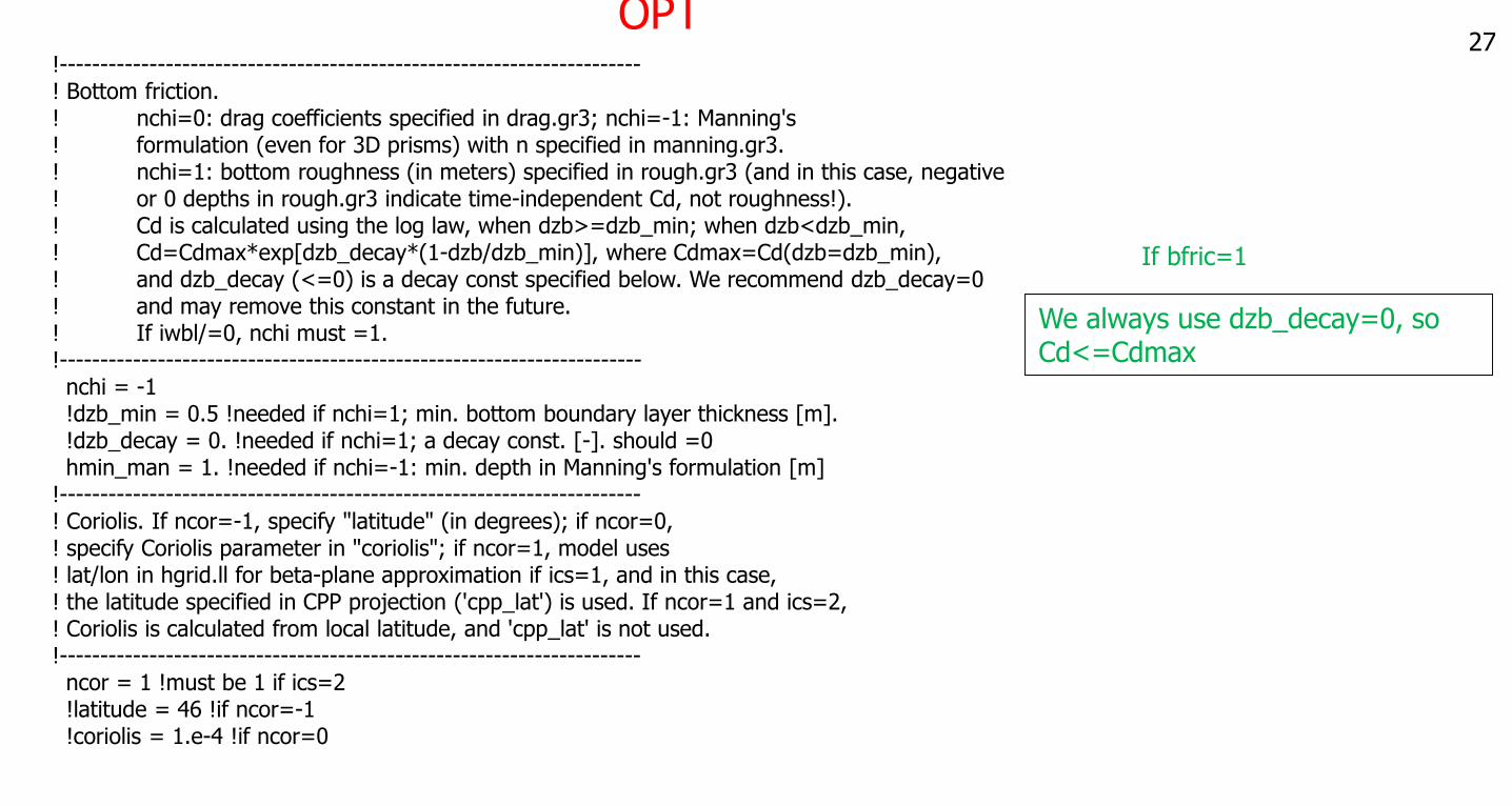
27OPT

We always use dzb_decay=0, so Cd<=Cdmax

If bfric=1

!-----------------------------------------------------------------------! Bottom friction.! nchi=0: drag coefficients specified in drag.gr3; nchi=-1: Manning's! formulation (even for 3D prisms) with n specified in manning.gr3.! nchi=1: bottom roughness (in meters) specified in rough.gr3 (and in this case, negative! or 0 depths in rough.gr3 indicate time-independent Cd, not roughness!).! Cd is calculated using the log law, when dzb>=dzb_min; when dzb<dzb_min,! Cd=Cdmax*exp[dzb_decay*(1-dzb/dzb_min)], where Cdmax=Cd(dzb=dzb_min),! and dzb_decay (<=0) is a decay const specified below. We recommend dzb_decay=0! and may remove this constant in the future.! If iwbl/=0, nchi must =1.!-----------------------------------------------------------------------nchi = -1!dzb_min = 0.5 !needed if nchi=1; min. bottom boundary layer thickness [m].!dzb_decay = 0. !needed if nchi=1; a decay const. [-]. should =0hmin_man = 1. !needed if nchi=-1: min. depth in Manning's formulation [m]

!-----------------------------------------------------------------------! Coriolis. If ncor=-1, specify "latitude" (in degrees); if ncor=0,! specify Coriolis parameter in "coriolis"; if ncor=1, model uses! lat/lon in hgrid.ll for beta-plane approximation if ics=1, and in this case,! the latitude specified in CPP projection ('cpp_lat') is used. If ncor=1 and ics=2,! Coriolis is calculated from local latitude, and 'cpp_lat' is not used.!-----------------------------------------------------------------------ncor = 1 !must be 1 if ics=2!latitude = 46 !if ncor=-1!coriolis = 1.e-4 !if ncor=0

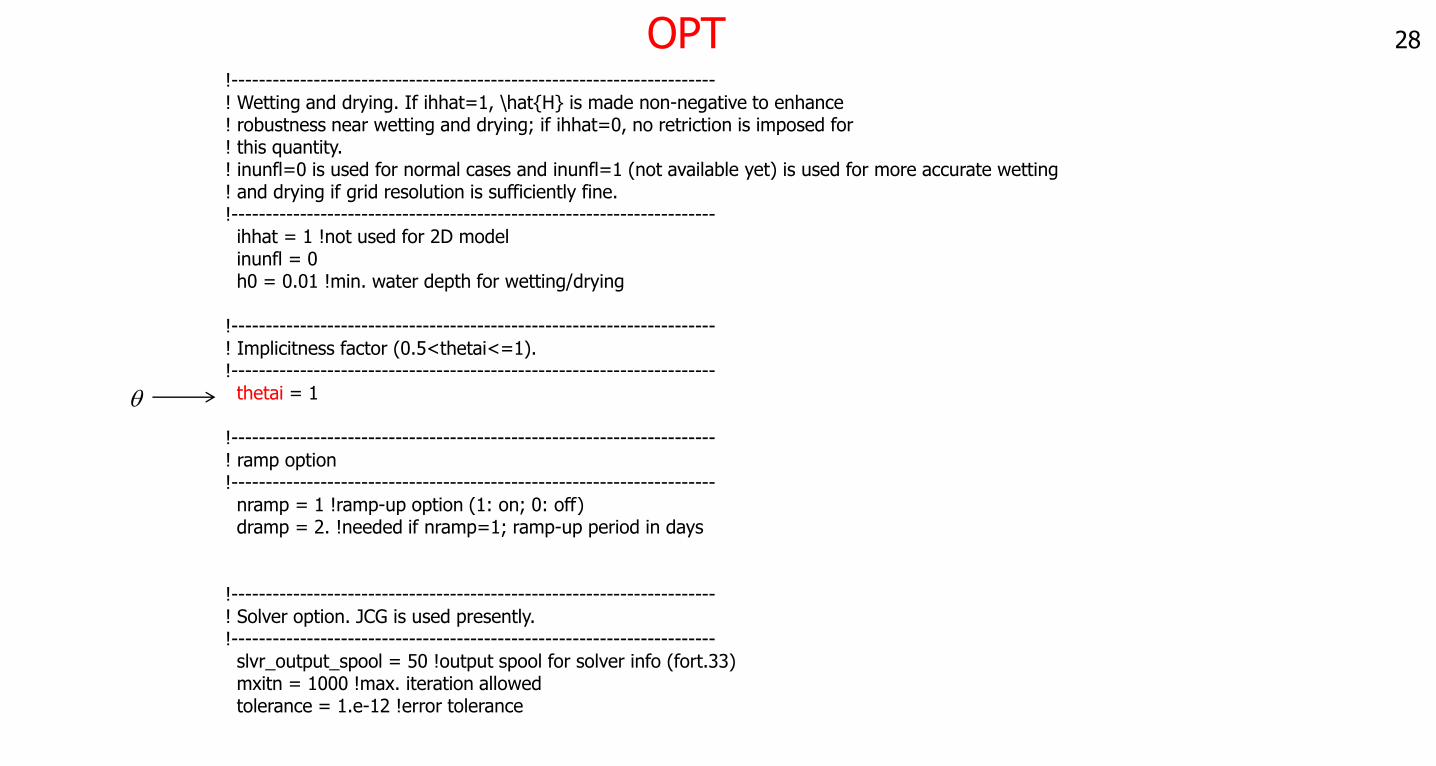
28OPT!-----------------------------------------------------------------------! Wetting and drying. If ihhat=1, \hat{H} is made non-negative to enhance! robustness near wetting and drying; if ihhat=0, no retriction is imposed for! this quantity.! inunfl=0 is used for normal cases and inunfl=1 (not available yet) is used for more accurate wetting! and drying if grid resolution is sufficiently fine.!-----------------------------------------------------------------------ihhat = 1 !not used for 2D modelinunfl = 0h0 = 0.01 !min. water depth for wetting/drying

!-----------------------------------------------------------------------! Implicitness factor (0.5<thetai<=1).!-----------------------------------------------------------------------thetai = 1

!-----------------------------------------------------------------------! ramp option!-----------------------------------------------------------------------nramp = 1 !ramp-up option (1: on; 0: off)dramp = 2. !needed if nramp=1; ramp-up period in days

!-----------------------------------------------------------------------! Solver option. JCG is used presently.!-----------------------------------------------------------------------slvr_output_spool = 50 !output spool for solver info (fort.33)mxitn = 1000 !max. iteration allowedtolerance = 1.e-12 !error tolerance

q

30OPT

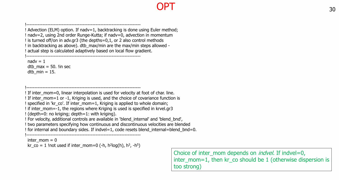
Choice of inter_mom depends on indvel. If indvel=0, inter_mom=1, then kr_co should be 1 (otherwise dispersion is too strong)

!-----------------------------------------------------------------------! Advection (ELM) option. If nadv=1, backtracking is done using Euler method;! nadv=2, using 2nd order Runge-Kutta; if nadv=0, advection in momentum! is turned off/on in adv.gr3 (the depths=0,1, or 2 also control methods! in backtracking as above). dtb_max/min are the max/min steps allowed -! actual step is calculated adaptively based on local flow gradient. !-----------------------------------------------------------------------nadv = 1dtb_max = 50. !in secdtb_min = 15.

!-----------------------------------------------------------------------! If inter_mom=0, linear interpolation is used for velocity at foot of char. line.! If inter_mom=1 or -1, Kriging is used, and the choice of covariance function is! specified in 'kr_co'. If inter_mom=1, Kriging is applied to whole domain;! if inter_mom=-1, the regions where Kriging is used is specified in krvel.gr3! (depth=0: no kriging; depth=1: with kriging).! For velocity, additional controls are available in 'blend_internal' and 'blend_bnd',! two parameters specifying how continuous and discontinuous velocities are blended! for internal and boundary sides. If indvel=1, code resets blend_internal=blend_bnd=0.!-----------------------------------------------------------------------inter_mom = 0kr_co = 1 !not used if inter_mom=0 (-h, h2log(h), h3, -h5)

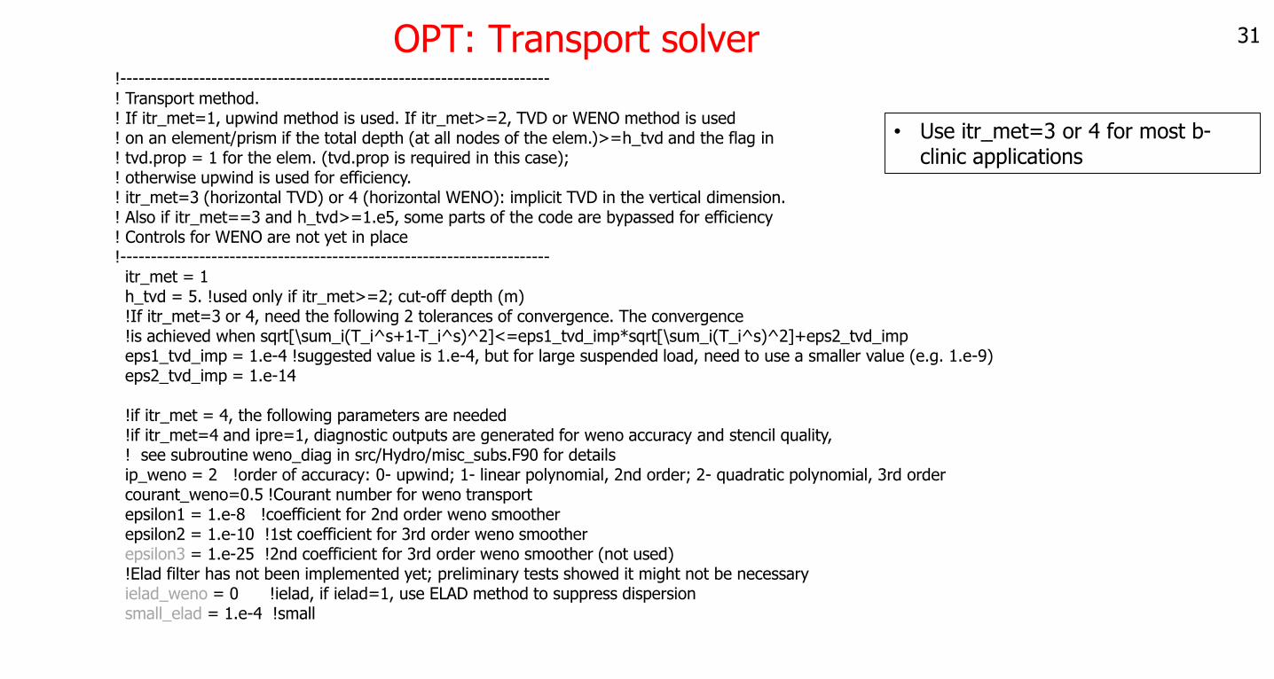
31OPT: Transport solver!-----------------------------------------------------------------------! Transport method.! If itr_met=1, upwind method is used. If itr_met>=2, TVD or WENO method is used! on an element/prism if the total depth (at all nodes of the elem.)>=h_tvd and the flag in! tvd.prop = 1 for the elem. (tvd.prop is required in this case);! otherwise upwind is used for efficiency.! itr_met=3 (horizontal TVD) or 4 (horizontal WENO): implicit TVD in the vertical dimension.! Also if itr_met==3 and h_tvd>=1.e5, some parts of the code are bypassed for efficiency! Controls for WENO are not yet in place!-----------------------------------------------------------------------itr_met = 1h_tvd = 5. !used only if itr_met>=2; cut-off depth (m)!If itr_met=3 or 4, need the following 2 tolerances of convergence. The convergence!is achieved when sqrt[\sum_i(T_i^s+1-T_i^s)^2]<=eps1_tvd_imp*sqrt[\sum_i(T_i^s)^2]+eps2_tvd_impeps1_tvd_imp = 1.e-4 !suggested value is 1.e-4, but for large suspended load, need to use a smaller value (e.g. 1.e-9)eps2_tvd_imp = 1.e-14

!if itr_met = 4, the following parameters are needed!if itr_met=4 and ipre=1, diagnostic outputs are generated for weno accuracy and stencil quality,! see subroutine weno_diag in src/Hydro/misc_subs.F90 for detailsip_weno = 2 !order of accuracy: 0- upwind; 1- linear polynomial, 2nd order; 2- quadratic polynomial, 3rd ordercourant_weno=0.5 !Courant number for weno transportepsilon1 = 1.e-8 !coefficient for 2nd order weno smootherepsilon2 = 1.e-10 !1st coefficient for 3rd order weno smootherepsilon3 = 1.e-25 !2nd coefficient for 3rd order weno smoother (not used)!Elad filter has not been implemented yet; preliminary tests showed it might not be necessaryielad_weno = 0 !ielad, if ielad=1, use ELAD method to suppress dispersionsmall_elad = 1.e-4 !small

• Use itr_met=3 or 4 for most b-clinic applications

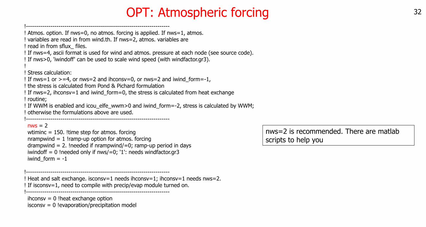
32OPT: Atmospheric forcing!-----------------------------------------------------------------------! Atmos. option. If nws=0, no atmos. forcing is applied. If nws=1, atmos.! variables are read in from wind.th. If nws=2, atmos. variables are! read in from sflux_ files.! If nws=4, ascii format is used for wind and atmos. pressure at each node (see source code).! If nws>0, 'iwindoff' can be used to scale wind speed (with windfactor.gr3).!! Stress calculation:! If nws=1 or >=4, or nws=2 and ihconsv=0, or nws=2 and iwind_form=-1,! the stress is calculated from Pond & Pichard formulation! If nws=2, ihconsv=1 and iwind_form=0, the stress is calculated from heat exchange! routine;! If WWM is enabled and icou_elfe_wwm>0 and iwind_form=-2, stress is calculated by WWM;! otherwise the formulations above are used.!-----------------------------------------------------------------------nws = 2wtiminc = 150. !time step for atmos. forcingnrampwind = 1 !ramp-up option for atmos. forcingdrampwind = 2. !needed if nrampwind/=0; ramp-up period in daysiwindoff = 0 !needed only if nws/=0; '1': needs windfactor.gr3iwind_form = -1

!-----------------------------------------------------------------------! Heat and salt exchange. isconsv=1 needs ihconsv=1; ihconsv=1 needs nws=2.! If isconsv=1, need to compile with precip/evap module turned on.!-----------------------------------------------------------------------ihconsv = 0 !heat exchange optionisconsv = 0 !evaporation/precipitation model

nws=2 is recommended. There are matlabscripts to help you

33

OPT: Turbulence closure

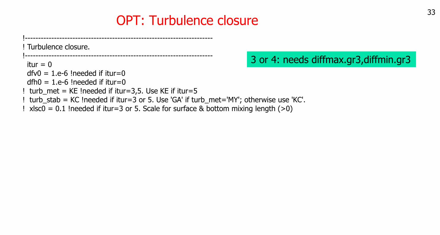
3 or 4: needs diffmax.gr3,diffmin.gr3

!-----------------------------------------------------------------------! Turbulence closure.!-----------------------------------------------------------------------

itur = 0dfv0 = 1.e-6 !needed if itur=0dfh0 = 1.e-6 !needed if itur=0

! turb_met = KE !needed if itur=3,5. Use KE if itur=5! turb_stab = KC !needed if itur=3 or 5. Use 'GA' if turb_met='MY'; otherwise use 'KC'.! xlsc0 = 0.1 !needed if itur=3 or 5. Scale for surface & bottom mixing length (>0)

34OPT

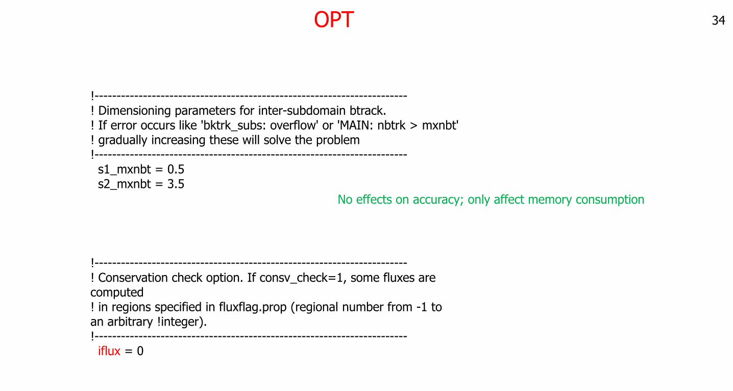
!-----------------------------------------------------------------------! Dimensioning parameters for inter-subdomain btrack.! If error occurs like 'bktrk_subs: overflow' or 'MAIN: nbtrk > mxnbt'! gradually increasing these will solve the problem!-----------------------------------------------------------------------

s1_mxnbt = 0.5s2_mxnbt = 3.5

No effects on accuracy; only affect memory consumption

!-----------------------------------------------------------------------! Conservation check option. If consv_check=1, some fluxes are computed! in regions specified in fluxflag.prop (regional number from -1 to an arbitrary !integer).!-----------------------------------------------------------------------

iflux = 0

35SCHOUT

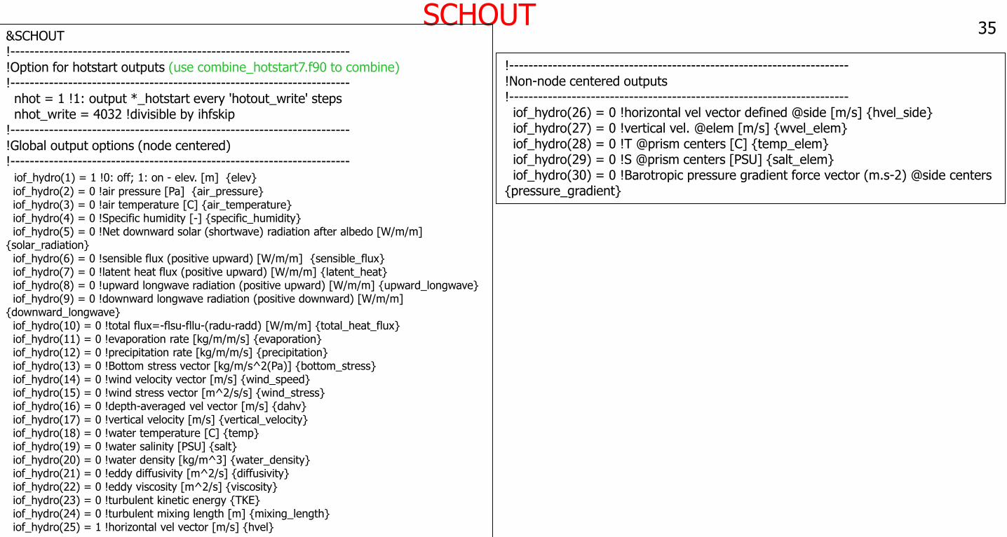
!-----------------------------------------------------------------------!Non-node centered outputs!-----------------------------------------------------------------------iof_hydro(26) = 0 !horizontal vel vector defined @side [m/s] {hvel_side}iof_hydro(27) = 0 !vertical vel. @elem [m/s] {wvel_elem}iof_hydro(28) = 0 !T @prism centers [C] {temp_elem}iof_hydro(29) = 0 !S @prism centers [PSU] {salt_elem}iof_hydro(30) = 0 !Barotropic pressure gradient force vector (m.s-2) @side centers

{pressure_gradient}

&SCHOUT!-----------------------------------------------------------------------!Option for hotstart outputs (use combine_hotstart7.f90 to combine)!-----------------------------------------------------------------------nhot = 1 !1: output *_hotstart every 'hotout_write' stepsnhot_write = 4032 !divisible by ihfskip

!-----------------------------------------------------------------------!Global output options (node centered)!-----------------------------------------------------------------------

iof_hydro(1) = 1 !0: off; 1: on - elev. [m] {elev}

iof_hydro(2) = 0 !air pressure [Pa] {air_pressure}iof_hydro(3) = 0 !air temperature [C] {air_temperature}iof_hydro(4) = 0 !Specific humidity [-] {specific_humidity}iof_hydro(5) = 0 !Net downward solar (shortwave) radiation after albedo [W/m/m]

{solar_radiation}iof_hydro(6) = 0 !sensible flux (positive upward) [W/m/m] {sensible_flux}iof_hydro(7) = 0 !latent heat flux (positive upward) [W/m/m] {latent_heat}iof_hydro(8) = 0 !upward longwave radiation (positive upward) [W/m/m] {upward_longwave}iof_hydro(9) = 0 !downward longwave radiation (positive downward) [W/m/m]

{downward_longwave}iof_hydro(10) = 0 !total flux=-flsu-fllu-(radu-radd) [W/m/m] {total_heat_flux}iof_hydro(11) = 0 !evaporation rate [kg/m/m/s] {evaporation}iof_hydro(12) = 0 !precipitation rate [kg/m/m/s] {precipitation}iof_hydro(13) = 0 !Bottom stress vector [kg/m/s^2(Pa)] {bottom_stress}iof_hydro(14) = 0 !wind velocity vector [m/s] {wind_speed}iof_hydro(15) = 0 !wind stress vector [m^2/s/s] {wind_stress}iof_hydro(16) = 0 !depth-averaged vel vector [m/s] {dahv}iof_hydro(17) = 0 !vertical velocity [m/s] {vertical_velocity}iof_hydro(18) = 0 !water temperature [C] {temp}iof_hydro(19) = 0 !water salinity [PSU] {salt}iof_hydro(20) = 0 !water density [kg/m^3] {water_density}iof_hydro(21) = 0 !eddy diffusivity [m^2/s] {diffusivity}iof_hydro(22) = 0 !eddy viscosity [m^2/s] {viscosity}iof_hydro(23) = 0 !turbulent kinetic energy {TKE}iof_hydro(24) = 0 !turbulent mixing length [m] {mixing_length}iof_hydro(25) = 1 !horizontal vel vector [m/s] {hvel}

36SCHOUT

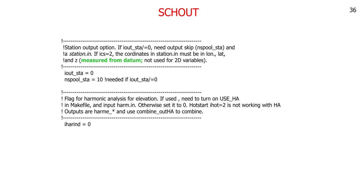
!-----------------------------------------------------------------------!Station output option. If iout_sta/=0, need output skip (nspool_sta) and!a station.in. If ics=2, the cordinates in station.in must be in lon., lat,!and z (measured from datum; not used for 2D variables).

!-----------------------------------------------------------------------iout_sta = 0nspool_sta = 10 !needed if iout_sta/=0

!-----------------------------------------------------------------------! Flag for harmonic analysis for elevation. If used , need to turn on USE_HA! in Makefile, and input harm.in. Otherwise set it to 0. Hotstart ihot=2 is not working with HA! Outputs are harme_* and use combine_outHA to combine.!-----------------------------------------------------------------------iharind = 0

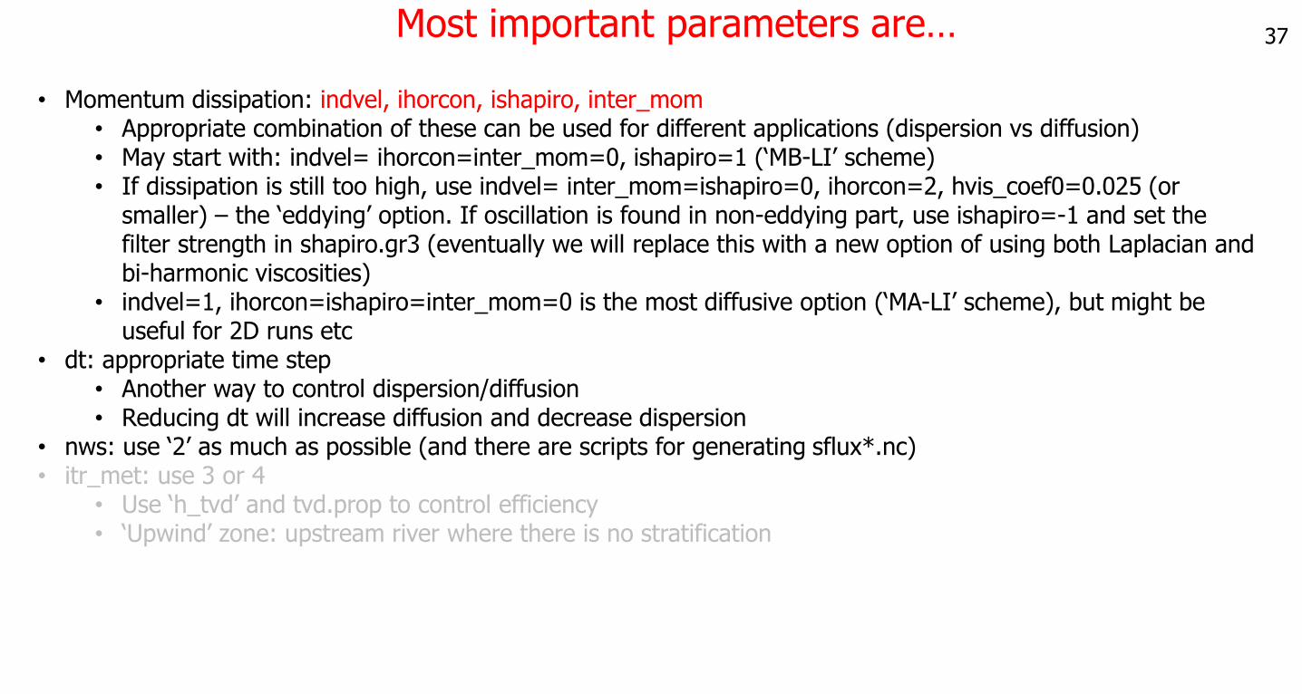
Most important parameters are…

• Momentum dissipation: indvel, ihorcon, ishapiro, inter_mom• Appropriate combination of these can be used for different applications (dispersion vs diffusion)• May start with: indvel= ihorcon=inter_mom=0, ishapiro=1 (‘MB-LI’ scheme)• If dissipation is still too high, use indvel= inter_mom=ishapiro=0, ihorcon=2, hvis_coef0=0.025 (or

smaller) – the ‘eddying’ option. If oscillation is found in non-eddying part, use ishapiro=-1 and set the filter strength in shapiro.gr3 (eventually we will replace this with a new option of using both Laplacian and bi-harmonic viscosities)

• indvel=1, ihorcon=ishapiro=inter_mom=0 is the most diffusive option (‘MA-LI’ scheme), but might be useful for 2D runs etc

• dt: appropriate time step • Another way to control dispersion/diffusion• Reducing dt will increase diffusion and decrease dispersion

• nws: use ‘2’ as much as possible (and there are scripts for generating sflux*.nc)• itr_met: use 3 or 4

• Use ‘h_tvd’ and tvd.prop to control efficiency• ‘Upwind’ zone: upstream river where there is no stratification

37

38Station.in

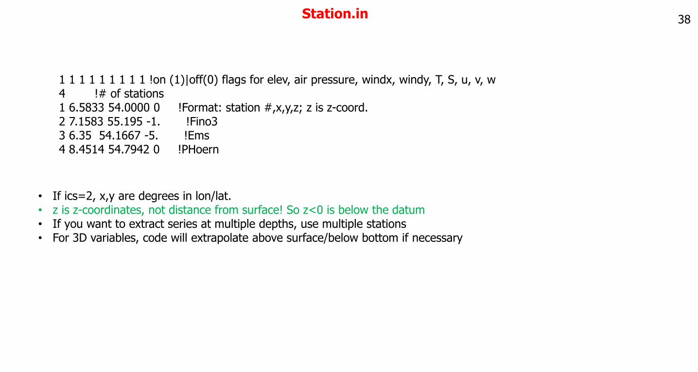
1 1 1 1 1 1 1 1 1 !on (1)|off(0) flags for elev, air pressure, windx, windy, T, S, u, v, w4 !# of stations1 6.5833 54.0000 0 !Format: station #,x,y,z; z is z-coord.2 7.1583 55.195 -1. !Fino33 6.35 54.1667 -5. !Ems4 8.4514 54.7942 0 !PHoern

• If ics=2, x,y are degrees in lon/lat.• z is z-coordinates, not distance from surface! So z<0 is below the datum• If you want to extract series at multiple depths, use multiple stations• For 3D variables, code will extrapolate above surface/below bottom if necessary

39Fluxflag.prop

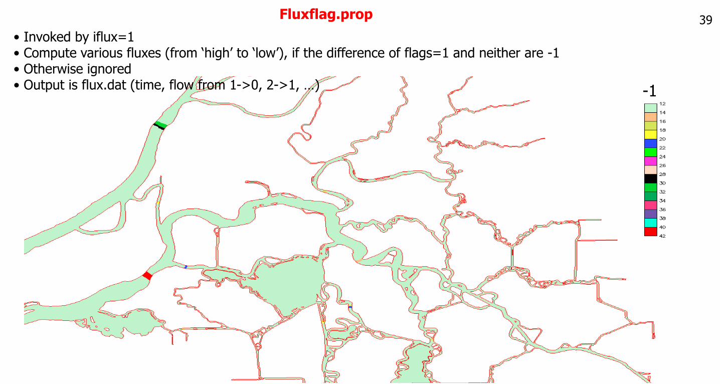
• Invoked by iflux=1• Compute various fluxes (from ‘high’ to ‘low’), if the difference of flags=1 and neither are -1 • Otherwise ignored• Output is flux.dat (time, flow from 1->0, 2->1, …) -1

40Hotstart and nuding inputs

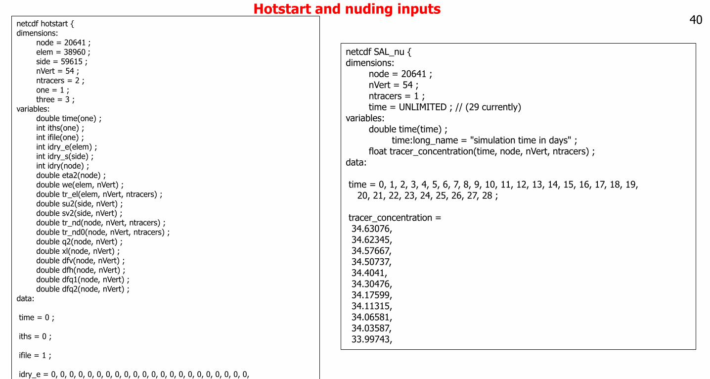
netcdf hotstart {dimensions:

node = 20641 ;elem = 38960 ;side = 59615 ;nVert = 54 ;ntracers = 2 ;one = 1 ;three = 3 ;

variables:double time(one) ;int iths(one) ;int ifile(one) ;int idry_e(elem) ;int idry_s(side) ;int idry(node) ;double eta2(node) ;double we(elem, nVert) ;double tr_el(elem, nVert, ntracers) ;double su2(side, nVert) ;double sv2(side, nVert) ;double tr_nd(node, nVert, ntracers) ;double tr_nd0(node, nVert, ntracers) ;double q2(node, nVert) ;double xl(node, nVert) ;double dfv(node, nVert) ;double dfh(node, nVert) ;double dfq1(node, nVert) ;double dfq2(node, nVert) ;

data:

time = 0 ;

iths = 0 ;

ifile = 1 ;

idry_e = 0, 0, 0, 0, 0, 0, 0, 0, 0, 0, 0, 0, 0, 0, 0, 0, 0, 0, 0, 0, 0, 0,

netcdf SAL_nu {dimensions:

node = 20641 ;nVert = 54 ;ntracers = 1 ;time = UNLIMITED ; // (29 currently)

variables:double time(time) ;

time:long_name = "simulation time in days" ;float tracer_concentration(time, node, nVert, ntracers) ;

data:

time = 0, 1, 2, 3, 4, 5, 6, 7, 8, 9, 10, 11, 12, 13, 14, 15, 16, 17, 18, 19,20, 21, 22, 23, 24, 25, 26, 27, 28 ;

tracer_concentration =34.63076,34.62345,34.57667,34.50737,34.4041,34.30476,34.17599,34.11315,34.06581,34.03587,33.99743,

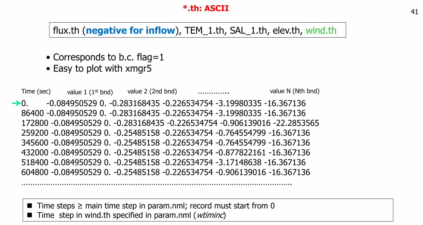
41*.th: ASCII

• Corresponds to b.c. flag=1• Easy to plot with xmgr5

Time (sec) value 1 (1st bnd) value 2 (2nd bnd) value N (Nth bnd)…………..

0. -0.084950529 0. -0.283168435 -0.226534754 -3.19980335 -16.36713686400 -0.084950529 0. -0.283168435 -0.226534754 -3.19980335 -16.367136172800 -0.084950529 0. -0.283168435 -0.226534754 -0.906139016 -22.2853565259200 -0.084950529 0. -0.25485158 -0.226534754 -0.764554799 -16.367136 345600 -0.084950529 0. -0.25485158 -0.226534754 -0.764554799 -16.367136 432000 -0.084950529 0. -0.25485158 -0.226534754 -0.877822161 -16.367136 518400 -0.084950529 0. -0.25485158 -0.226534754 -3.17148638 -16.367136604800 -0.084950529 0. -0.25485158 -0.226534754 -0.906139016 -16.367136………………………………………………………………………………………………………….

Time steps ≥ main time step in param.nml; record must start from 0 Time step in wind.th specified in param.nml (wtiminc)

flux.th (negative for inflow), TEM_1.th, SAL_1.th, elev.th, wind.th

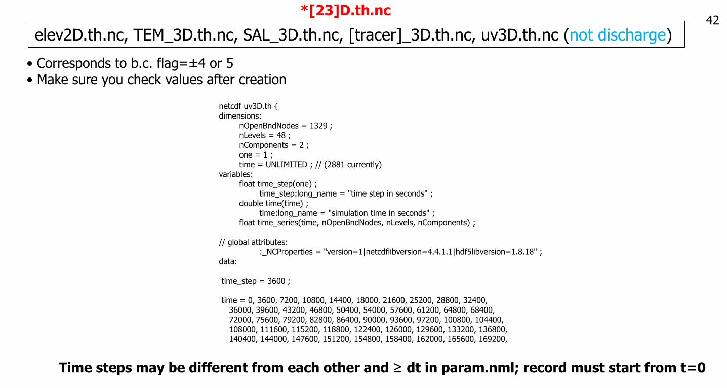
42*[23]D.th.nc

• Corresponds to b.c. flag=±4 or 5• Make sure you check values after creation

elev2D.th.nc, TEM_3D.th.nc, SAL_3D.th.nc, [tracer]_3D.th.nc, uv3D.th.nc (not discharge)

Time steps may be different from each other and ≥ dt in param.nml; record must start from t=0

netcdf uv3D.th {dimensions:

nOpenBndNodes = 1329 ;nLevels = 48 ;nComponents = 2 ;one = 1 ;time = UNLIMITED ; // (2881 currently)

variables:float time_step(one) ;

time_step:long_name = "time step in seconds" ;double time(time) ;

time:long_name = "simulation time in seconds" ;float time_series(time, nOpenBndNodes, nLevels, nComponents) ;

// global attributes::_NCProperties = "version=1|netcdflibversion=4.4.1.1|hdf5libversion=1.8.18" ;

data:

time_step = 3600 ;

time = 0, 3600, 7200, 10800, 14400, 18000, 21600, 25200, 28800, 32400,36000, 39600, 43200, 46800, 50400, 54000, 57600, 61200, 64800, 68400,72000, 75600, 79200, 82800, 86400, 90000, 93600, 97200, 100800, 104400,108000, 111600, 115200, 118800, 122400, 126000, 129600, 133200, 136800,140400, 144000, 147600, 151200, 154800, 158400, 162000, 165600, 169200,

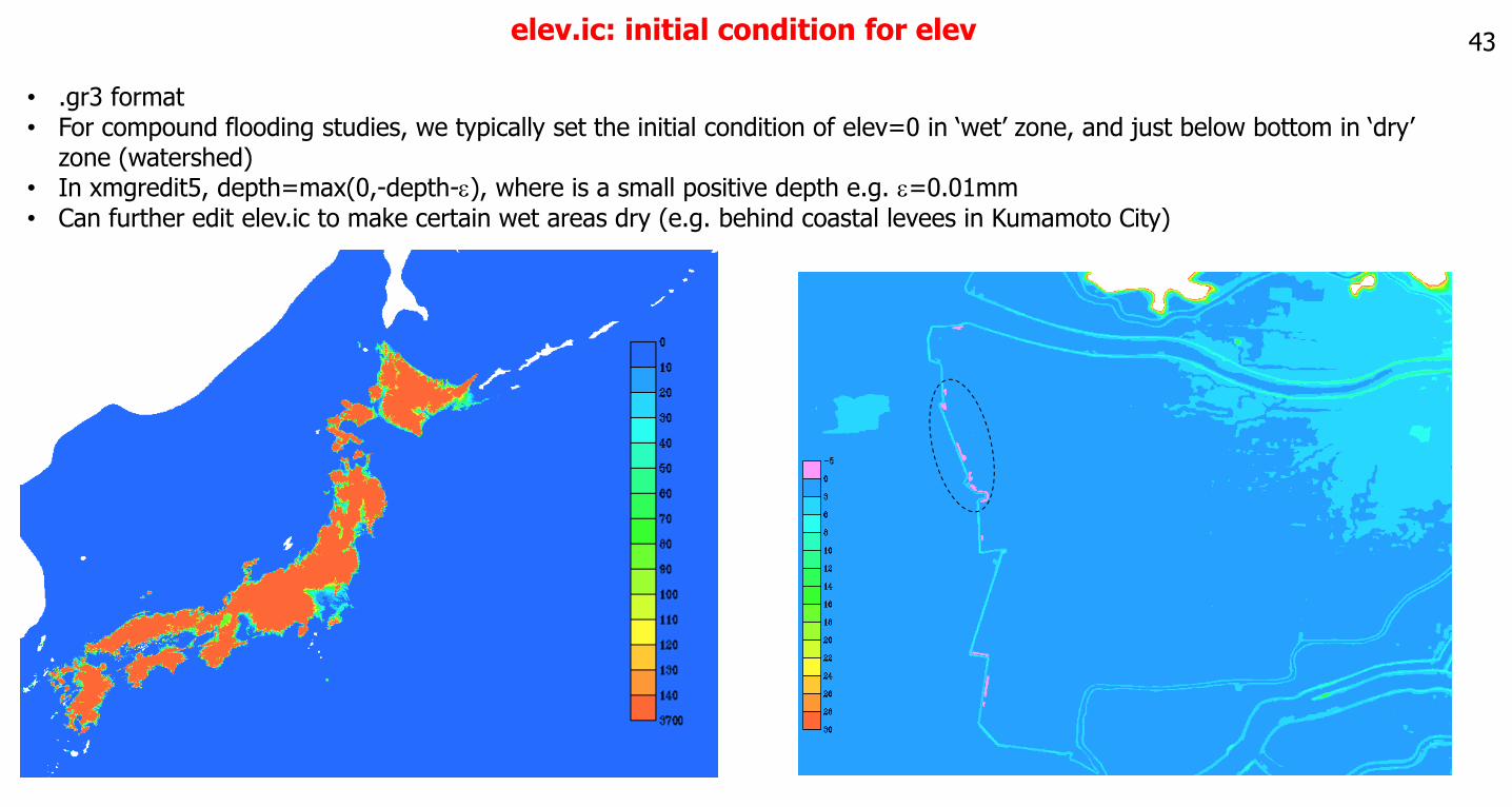
43elev.ic: initial condition for elev

• .gr3 format• For compound flooding studies, we typically set the initial condition of elev=0 in ‘wet’ zone, and just below bottom in ‘dry’

zone (watershed)• In xmgredit5, depth=max(0,-depth-e), where is a small positive depth e.g. e=0.01mm• Can further edit elev.ic to make certain wet areas dry (e.g. behind coastal levees in Kumamoto City)

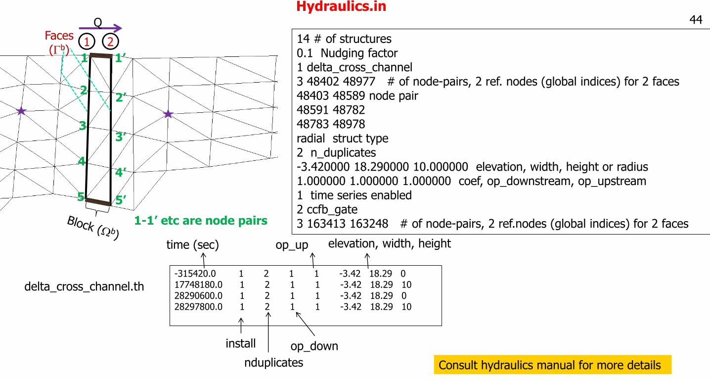
Hydraulics.in

14 # of structures0.1 Nudging factor1 delta_cross_channel3 48402 48977 # of node-pairs, 2 ref. nodes (global indices) for 2 faces48403 48589 node pair48591 4878248783 48978radial struct type2 n_duplicates-3.420000 18.290000 10.000000 elevation, width, height or radius1.000000 1.000000 1.000000 coef, op_downstream, op_upstream1 time series enabled2 ccfb_gate3 163413 163248 # of node-pairs, 2 ref.nodes (global indices) for 2 faces

-315420.0 1 2 1 1 -3.42 18.29 017748180.0 1 2 1 1 -3.42 18.29 1028290600.0 1 2 1 1 -3.42 18.29 028297800.0 1 2 1 1 -3.42 18.29 10

delta_cross_channel.th

install

nduplicates

op_down

op_up elevation, width, height time (sec)

Consult hydraulics manual for more details

1 2

QFaces (Gb)

1

2

3

4

5 5’

4’

3’

2’

1’

1-1’ etc are node pairs

44

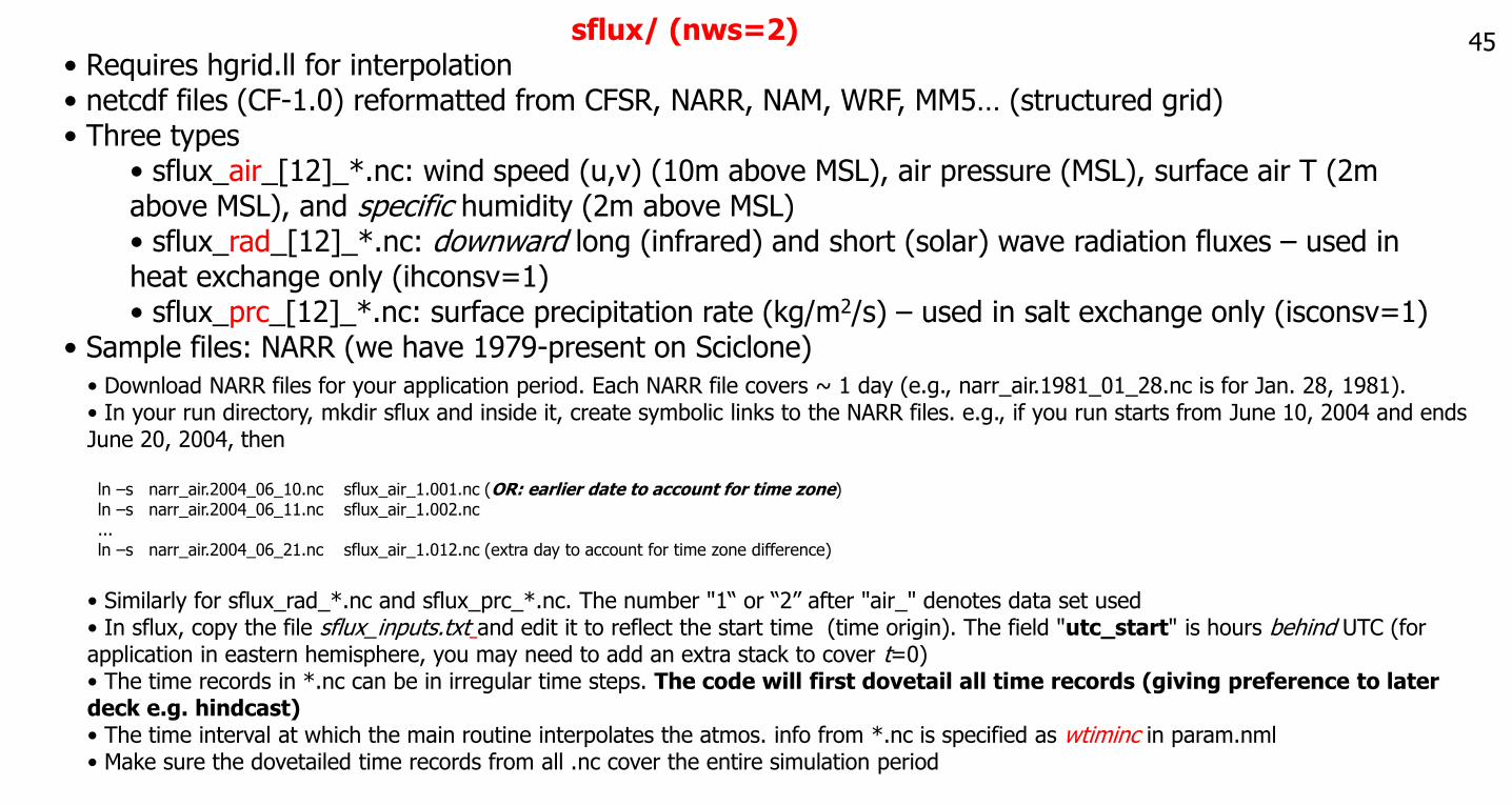
45sflux/ (nws=2)• Requires hgrid.ll for interpolation• netcdf files (CF-1.0) reformatted from CFSR, NARR, NAM, WRF, MM5… (structured grid)• Three types

• sflux_air_[12]_*.nc: wind speed (u,v) (10m above MSL), air pressure (MSL), surface air T (2m above MSL), and specific humidity (2m above MSL)• sflux_rad_[12]_*.nc: downward long (infrared) and short (solar) wave radiation fluxes – used in heat exchange only (ihconsv=1)• sflux_prc_[12]_*.nc: surface precipitation rate (kg/m2/s) – used in salt exchange only (isconsv=1)

• Sample files: NARR (we have 1979-present on Sciclone)

• Download NARR files for your application period. Each NARR file covers ~ 1 day (e.g., narr_air.1981_01_28.nc is for Jan. 28, 1981). • In your run directory, mkdir sflux and inside it, create symbolic links to the NARR files. e.g., if you run starts from June 10, 2004 and ends June 20, 2004, then

ln –s narr_air.2004_06_10.nc sflux_air_1.001.nc (OR: earlier date to account for time zone)ln –s narr_air.2004_06_11.nc sflux_air_1.002.nc ... ln –s narr_air.2004_06_21.nc sflux_air_1.012.nc (extra day to account for time zone difference)

• Similarly for sflux_rad_*.nc and sflux_prc_*.nc. The number "1“ or “2” after "air_" denotes data set used• In sflux, copy the file sflux_inputs.txt and edit it to reflect the start time (time origin). The field "utc_start" is hours behind UTC (for application in eastern hemisphere, you may need to add an extra stack to cover t=0)• The time records in *.nc can be in irregular time steps. The code will first dovetail all time records (giving preference to later deck e.g. hindcast)• The time interval at which the main routine interpolates the atmos. info from *.nc is specified as wtiminc in param.nml• Make sure the dovetailed time records from all .nc cover the entire simulation period

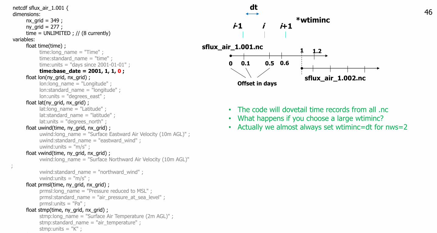
46netcdf sflux_air_1.001 {dimensions:

nx_grid = 349 ;ny_grid = 277 ;time = UNLIMITED ; // (8 currently)

variables:float time(time) ;

time:long_name = "Time" ;time:standard_name = "time" ;time:units = "days since 2001-01-01" ;time:base_date = 2001, 1, 1, 0 ;

float lon(ny_grid, nx_grid) ;lon:long_name = "Longitude" ;lon:standard_name = "longitude" ;lon:units = "degrees_east" ;

float lat(ny_grid, nx_grid) ;lat:long_name = "Latitude" ;lat:standard_name = "latitude" ;lat:units = "degrees_north" ;

float uwind(time, ny_grid, nx_grid) ;uwind:long_name = "Surface Eastward Air Velocity (10m AGL)" ;uwind:standard_name = "eastward_wind" ; uwind:units = "m/s" ;

float vwind(time, ny_grid, nx_grid) ;vwind:long_name = "Surface Northward Air Velocity (10m AGL)"

;vwind:standard_name = "northward_wind" ; vwind:units = "m/s" ;

float prmsl(time, ny_grid, nx_grid) ;prmsl:long_name = "Pressure reduced to MSL" ;prmsl:standard_name = "air_pressure_at_sea_level" ;prmsl:units = "Pa" ;

float stmp(time, ny_grid, nx_grid) ;stmp:long_name = "Surface Air Temperature (2m AGL)" ;stmp:standard_name = "air_temperature" ;stmp:units = "K" ;

float spfh(time, ny_grid, nx_grid) ;

sflux_air_1.001.nc

sflux_air_1.002.ncOffset in days

0 0.1 0.5 0.6

1 1.2

• The code will dovetail time records from all .nc• What happens if you choose a large wtiminc? • Actually we almost always set wtiminc=dt for nws=2

i-1 i i+1*wtiminc

dt

47Details: interpolation

sflux_air_1

Sflux_air_2

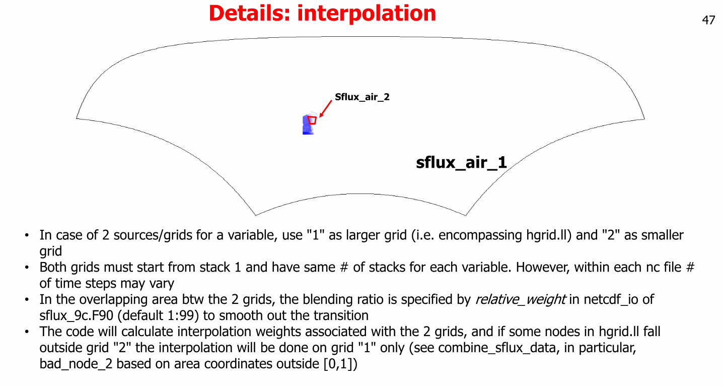
• In case of 2 sources/grids for a variable, use "1" as larger grid (i.e. encompassing hgrid.ll) and "2" as smaller grid

• Both grids must start from stack 1 and have same # of stacks for each variable. However, within each nc file # of time steps may vary

• In the overlapping area btw the 2 grids, the blending ratio is specified by relative_weight in netcdf_io of sflux_9c.F90 (default 1:99) to smooth out the transition

• The code will calculate interpolation weights associated with the 2 grids, and if some nodes in hgrid.ll fall outside grid "2" the interpolation will be done on grid "1" only (see combine_sflux_data, in particular, bad_node_2 based on area coordinates outside [0,1])

Creating your own sflux/

o Sample m-lab scripts: readnc*.mo The grids used in atmospheric forcings are structured grids, but atmos grid “1” must

encompass hgrid.ll for successful interpolation, which is done in SCHISM at run time (both in space and in time)o The collective time window from all .nc files MUST cover the simulation period

o Of all attributes in nc file, only 'base_date' is required (hour is not used)o Grids for air, rad and prc can be different (but must be the same within each type and each

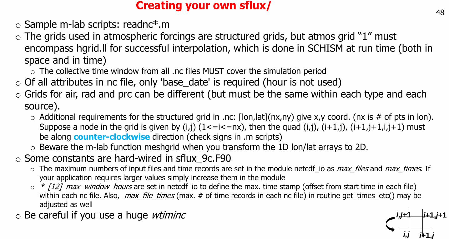
source). o Additional requirements for the structured grid in .nc: [lon,lat](nx,ny) give x,y coord. (nx is # of pts in lon).

Suppose a node in the grid is given by (i,j) (1<=i<=nx), then the quad (i,j), (i+1,j), (i+1,j+1,i,j+1) must be along counter-clockwise direction (check signs in .m scripts)

o Beware the m-lab function meshgrid when you transform the 1D lon/lat arrays to 2D.

o Some constants are hard-wired in sflux_9c.F90o The maximum numbers of input files and time records are set in the module netcdf_io as max_files and max_times. If

your application requires larger values simply increase them in the moduleo *_[12]_max_window_hours are set in netcdf_io to define the max. time stamp (offset from start time in each file)

within each nc file. Also, max_file_times (max. # of time records in each nc file) in routine get_times_etc() may be adjusted as well

o Be careful if you use a huge wtiminc

i,j i+1,j

i,j+1 i+1,j+1

48

49Particle tracking

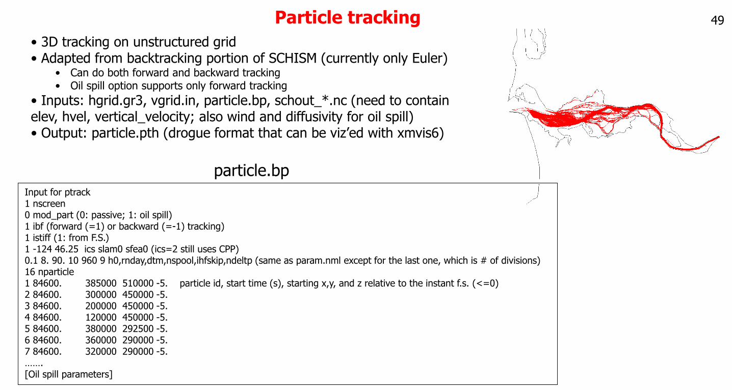
• 3D tracking on unstructured grid• Adapted from backtracking portion of SCHISM (currently only Euler)

• Can do both forward and backward tracking• Oil spill option supports only forward tracking

• Inputs: hgrid.gr3, vgrid.in, particle.bp, schout_*.nc (need to contain elev, hvel, vertical_velocity; also wind and diffusivity for oil spill)• Output: particle.pth (drogue format that can be viz’ed with xmvis6)

Input for ptrack1 nscreen0 mod_part (0: passive; 1: oil spill)1 ibf (forward (=1) or backward (=-1) tracking)1 istiff (1: from F.S.)1 -124 46.25 ics slam0 sfea0 (ics=2 still uses CPP)0.1 8. 90. 10 960 9 h0,rnday,dtm,nspool,ihfskip,ndeltp (same as param.nml except for the last one, which is # of divisions) 16 nparticle1 84600. 385000 510000 -5. particle id, start time (s), starting x,y, and z relative to the instant f.s. (<=0)2 84600. 300000 450000 -5.3 84600. 200000 450000 -5.4 84600. 120000 450000 -5.5 84600. 380000 292500 -5.6 84600. 360000 290000 -5.7 84600. 320000 290000 -5.…….[Oil spill parameters]

particle.bp

Advanced topics

50

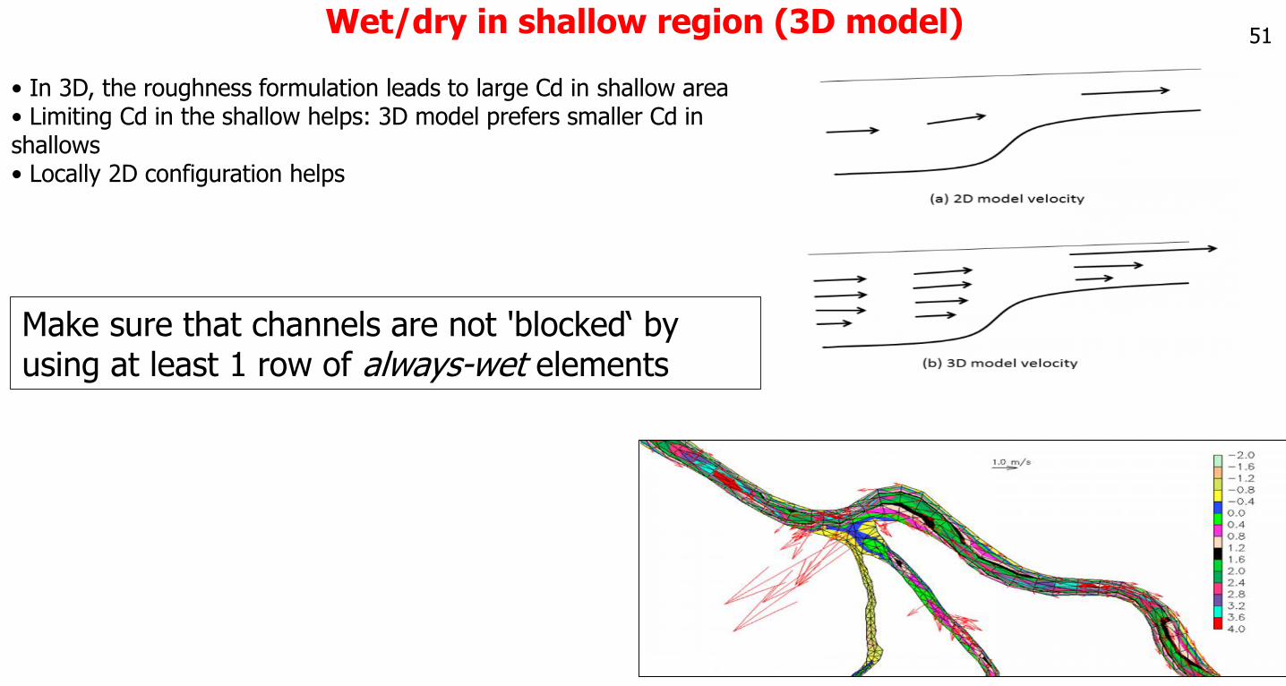
51Wet/dry in shallow region (3D model)

• In 3D, the roughness formulation leads to large Cd in shallow area • Limiting Cd in the shallow helps: 3D model prefers smaller Cd in shallows• Locally 2D configuration helps

Make sure that channels are not 'blocked‘ by using at least 1 row of always-wet elements

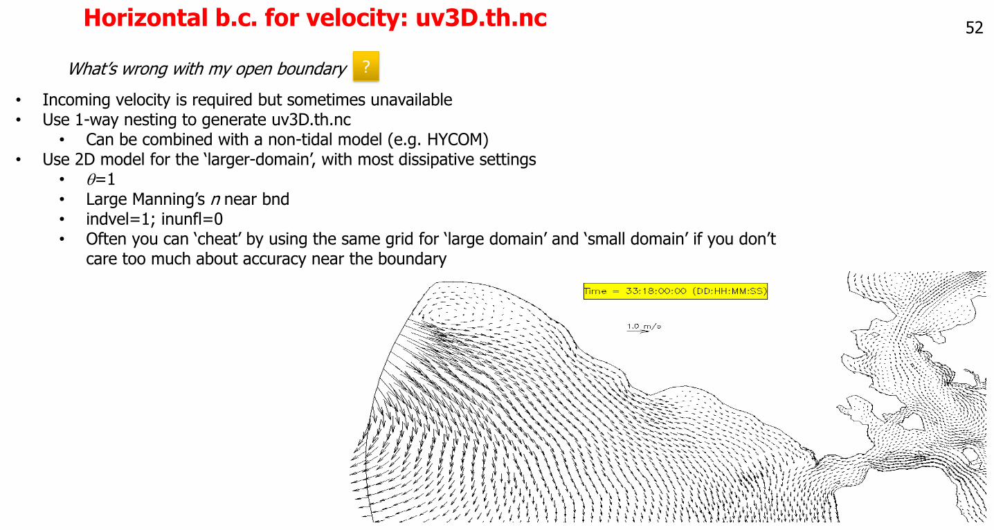
Horizontal b.c. for velocity: uv3D.th.nc

What’s wrong with my open boundary ?

• Incoming velocity is required but sometimes unavailable• Use 1-way nesting to generate uv3D.th.nc

• Can be combined with a non-tidal model (e.g. HYCOM)• Use 2D model for the ‘larger-domain’, with most dissipative settings

• q=1• Large Manning’s n near bnd• indvel=1; inunfl=0• Often you can ‘cheat’ by using the same grid for ‘large domain’ and ‘small domain’ if you don’t

care too much about accuracy near the boundary

52

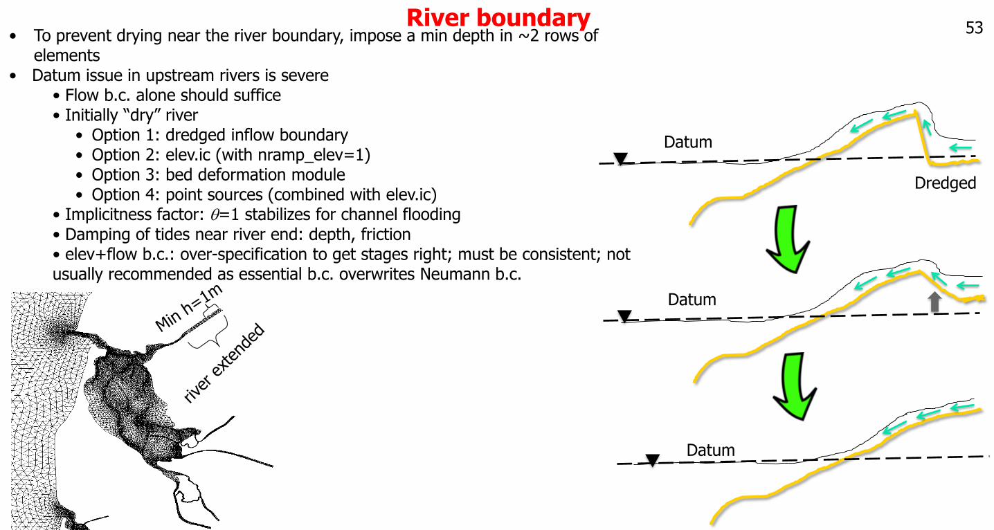
River boundary• To prevent drying near the river boundary, impose a min depth in ~2 rows of

elements• Datum issue in upstream rivers is severe

• Flow b.c. alone should suffice • Initially “dry” river

• Option 1: dredged inflow boundary• Option 2: elev.ic (with nramp_elev=1)• Option 3: bed deformation module • Option 4: point sources (combined with elev.ic)

• Implicitness factor: q=1 stabilizes for channel flooding• Damping of tides near river end: depth, friction• elev+flow b.c.: over-specification to get stages right; must be consistent; not usually recommended as essential b.c. overwrites Neumann b.c.

Datum

Datum

Dredged

Datum

53

Add tides

• HYCOM does not have tides (actually it may be better to explicitly filter out any high-frequency signals in it)• Tidal signals are added into HYCOM SSH and u,v at the boundary

• Tidal potential should be added in the interior of the domain • Add tidal elevation

• Use iettype=5: tidal amplitudes/phases are specified in bctides.in, whereas non-tidal HYCOM is in elev2D.th.nc

• Add tidal velocity • Use ifltype=5: tidal amplitudes/phases are specified in bctides.in, whereas non-tidal HYCOM is in

uv3D.th.nc• Since the velocity is never perfect at the boundary, the tracer concentration needs to be nudged in a zone near

the ocean boundary• The incoming vel is more important, especially for indvel=0 which has lower dissipation and thus requires

more stabilization

54

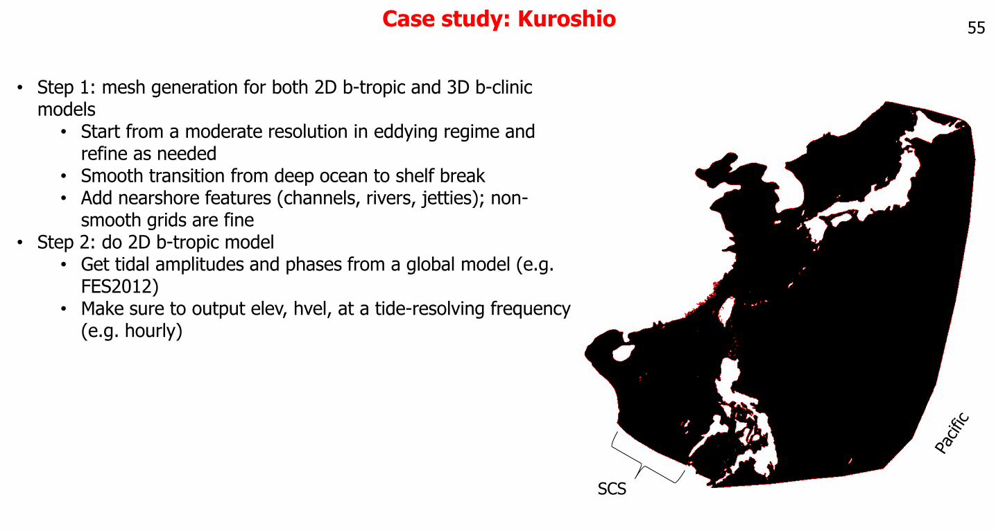
Case study: Kuroshio

• Step 1: mesh generation for both 2D b-tropic and 3D b-clinic models

• Start from a moderate resolution in eddying regime and refine as needed

• Smooth transition from deep ocean to shelf break• Add nearshore features (channels, rivers, jetties); non-

smooth grids are fine• Step 2: do 2D b-tropic model

• Get tidal amplitudes and phases from a global model (e.g. FES2012)

• Make sure to output elev, hvel, at a tide-resolving frequency (e.g. hourly)

SCS

55

Recap…

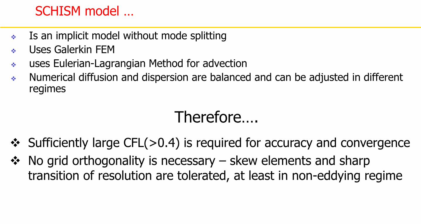
SCHISM model …

Is an implicit model without mode splitting

Uses Galerkin FEM

uses Eulerian-Lagrangian Method for advection

Numerical diffusion and dispersion are balanced and can be adjusted in different regimes

Therefore….

Sufficiently large CFL(>0.4) is required for accuracy and convergence

No grid orthogonality is necessary – skew elements and sharp transition of resolution are tolerated, at least in non-eddying regime

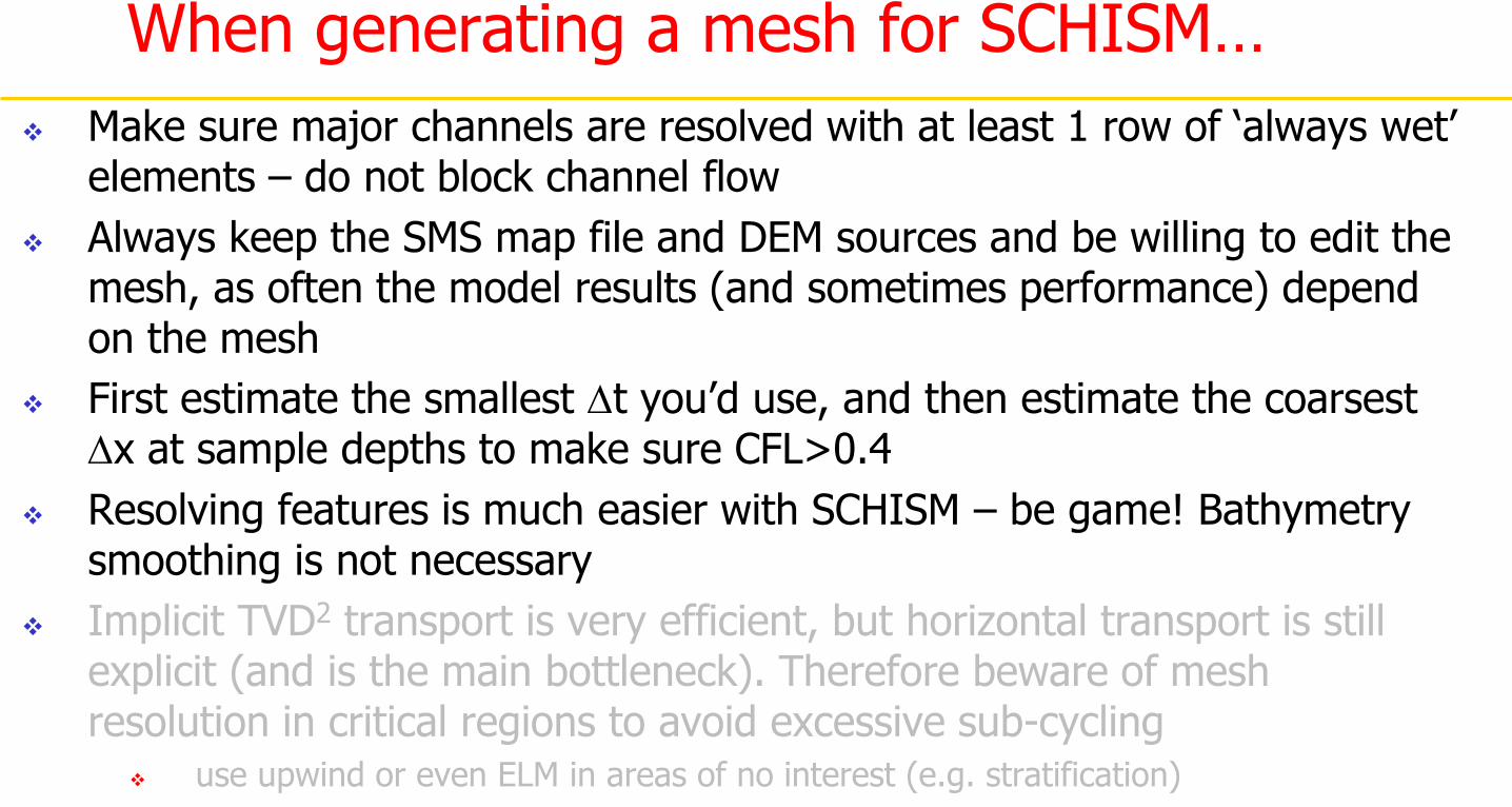
When generating a mesh for SCHISM…

Make sure major channels are resolved with at least 1 row of ‘always wet’ elements – do not block channel flow

Always keep the SMS map file and DEM sources and be willing to edit the mesh, as often the model results (and sometimes performance) depend on the mesh

First estimate the smallest Dt you’d use, and then estimate the coarsest Dx at sample depths to make sure CFL>0.4

Resolving features is much easier with SCHISM – be game! Bathymetry smoothing is not necessary

Implicit TVD2 transport is very efficient, but horizontal transport is still explicit (and is the main bottleneck). Therefore beware of mesh resolution in critical regions to avoid excessive sub-cycling

use upwind or even ELM in areas of no interest (e.g. stratification)

When setting up a model…

Always check the mesh first with a simple 2D model with ipre=1 The model is very adept at checking integrity of inputs

Start from simple and then build up complexity

Examine surface velocity in animation mode to find potential issues

Avoid large CD in very shallow areas in 3D regions

Make sure open boundaries do not become completely dry (partial dry is fine)

Negative river flow for inflow

When calibrating SCHISM…

Remember the mesh is the single most important factor for accuracy – here lies the greatest strength and challenge of unstructured grids

Control the balance between numerical diffusion and dispersion (indvel, ihorcon…)

Transport solver performance may require some experience

LSC2 grid requires some learning, but is a very powerful tool (resembling unstructured grid in the vertical)

User support

1. Online manual

2. Test suite on svn

3. Register on schism.wiki and send a ticket to user mailing list