EL 625 Lecture 4 1

EL 625 Lecture 4

Solution of the dynamic state equations

x(t) = A(t)x(t) + B(t)u(t)

y(t) = C(t)x(t) + D(t)u(t) (1)

Homogeneous equation (Unforced system):

x = A(t)x (2)

Consider the matrix differential equation, Q(t) = A(t)Q(t). If

this can be solved, the solution to the homogeneous equation is

x(t) = Q(t)Q−1(t0)x(t0) (3)

x(t) = Q(t)Q−1(t0)x(t0)

= A(t)Q(t)Q−1(t0)x(t0)

= A(t)x(t) (4)

Also, evaluating the left side of (3) at t = t0, we have

Q(t0)Q−1(t0)x(t0) = x(t0) (5)

So, the solution satisfies the initial condition.

EL 625 Lecture 4 2

‘Transition matrix’, φ(t, t0) =4 Q(t)Q−1(t0) (6)

x(t) = φ(t, t0)x(t0) (7)

The transition matrix characterizes the ‘flow’ of the differential e-

quation.

Properties of the transition matrix:

1. x(t0) = φ(t0, t0)x(t0)

φ(t0, t0) = I (8)

2.

φ(t2, t0)x(t0) = x(t2)

= φ(t2, t1)x(t1)

= φ(t2, t1)φ(t1, t0)x(t0)

φ(t2, t1)φ(t1, t0) = φ(t2, t0) (9)

3.

x(t2) = φ(t2, t1)x(t1) = φ(t2, t1)φ(t1, t2)x(t2)

EL 625 Lecture 4 3

φ(t2, t1)φ(t1, t2) = I (10)

φ(t1, t2) = φ−1(t2, t1) (11)

Given a transition matrix, φ(t, t0), A(t) can be evaluated as follows.

x(t) = φ(t, t0)x(t0)

Also, x(t) = A(t)x(t)

= A(t)φ(t, t0)x(t0)

φ(t, t0) = A(t)φ(t, t0) (12)

φ(t, t0)|t0=t = A(t) (13)

We can also determine an expression for φ−1(t, t0).

φ(t, t0)φ−1(t, t0) = I (14)

ddtφ(t, t0)

φ−1(t, t0) + φ(t, t0)

ddtφ−1(t, t0)

= 0 (15)

ddtφ(t, t0)

φ−1(t, t0) = −φ(t, t0)

ddtφ−1(t, t0)

ddtφ−1(t, t0) = −φ−1(t, t0)

ddtφ(t, t0)

φ−1(t, t0)

= −φ−1(t, t0)A(t)φ(t, t0)φ−1(t, t0)

= −φ−1(t, t0)A(t) (16)

EL 625 Lecture 4 4

Solution of the forced system equations:

Assume:

x(t) = φ(t, t0)f(t) (17)

=⇒

x(t) = φ(t, t0)f(t) + φ(t, t0)f(t)

= A(t)φ(t, t0)f(t) + φ(t, t0)f(t)

= A(t)x(t) + φ(t, t0)f(t)

=⇒ φ(t, t0)f(t) = B(t)u(t) (18)

Thus,

f(t) = f(t0) +∫ t

t0φ(t0, λ)B(λ)u(λ)dλ (19)

x(t) = φ(t, t0)f(t0) +∫ t

t0φ(t, t0)φ(t0, λ)B(λ)u(λ)dλ (20)

x(t) = φ(t, t0)x(t0) +∫ t

t0φ(t, λ)B(λ)u(λ)dλ (21)

EL 625 Lecture 4 5

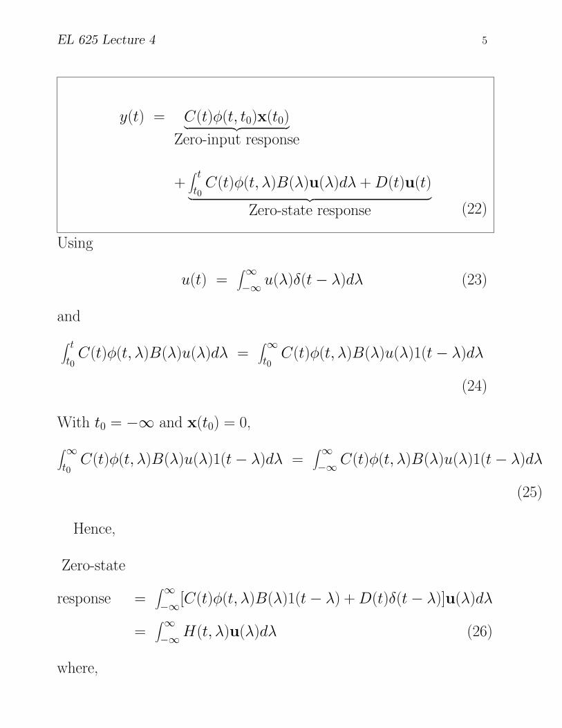
y(t) = C(t)φ(t, t0)x(t0)︸ ︷︷ ︸

Zero-input response

+∫ t

t0C(t)φ(t, λ)B(λ)u(λ)dλ +D(t)u(t)

︸ ︷︷ ︸

Zero-state response (22)

Using

u(t) =∫ ∞−∞ u(λ)δ(t− λ)dλ (23)

and∫ t

t0C(t)φ(t, λ)B(λ)u(λ)dλ =

∫ ∞t0C(t)φ(t, λ)B(λ)u(λ)1(t− λ)dλ

(24)

With t0 = −∞ and x(t0) = 0,∫ ∞t0C(t)φ(t, λ)B(λ)u(λ)1(t− λ)dλ =

∫ ∞−∞C(t)φ(t, λ)B(λ)u(λ)1(t− λ)dλ

(25)

Hence,

Zero-state

response =∫ ∞−∞[C(t)φ(t, λ)B(λ)1(t− λ) + D(t)δ(t− λ)]u(λ)dλ

=∫ ∞−∞H(t, λ)u(λ)dλ (26)

where,

EL 625 Lecture 4 6

H(t, λ) = C(t)φ(t, λ)B(λ)1(t− λ) + D(t)δ(t− λ)

For fixed systems, A,B,C and D are constant matrices

H(t, λ) = H(t− λ) (27)

H(t) = Cφ(t)B1(t) + Dδ(t) (28)

A different approach to the derivation of the forced response

x(t) = A(t)x(t) + B(t)u(t)

φ(t0, t)x(t) = φ(t0, t)A(t)x(t) + φ(t0, t)B(t)u(t)

φ(t0, t)x(t)− φ(t0, t)A(t)x(t) = φ(t0, t)B(t)u(t)

φ(t0, t)x(t) + φ(t0, t)x(t) = φ(t0, t)B(t)u(t) (29)ddt

(φ(t0, t)x(t)) = φ(t0, t)B(t)u(t) (30)

φ(t0, τ )x(t)|tτ=t0 =∫ t

t0φ(t0, τ )B(τ )u(τ )dτ (31)

φ(t0, t)x(t)− x(t0) =∫ t

t0φ(t0, τ )B(τ )u(τ )dτ (32)

φ(t0, t)x(t) = x(t0) +∫ t

t0φ(t0, τ )B(τ )u(τ )dτ(33)

x(t) = φ(t, t0)x(t0)

+φ(t, t0)∫ t

t0φ(t0, τ )B(τ )u(τ )dτ(34)

EL 625 Lecture 4 7

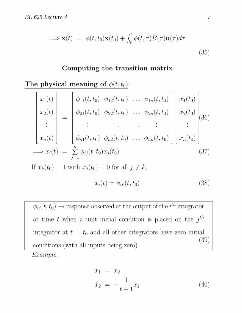
=⇒ x(t) = φ(t, t0)x(t0) +∫ t

t0φ(t, τ )B(τ )u(τ )dτ

(35)

Computing the transition matrix

The physical meaning of φ(t, t0):

x1(t)

x2(t)...

xn(t)

=

φ11(t, t0) φ12(t, t0) . . . φ1n(t, t0)

φ21(t, t0) φ22(t, t0) . . . φ2n(t, t0)... . . . . . . ...

φn1(t, t0) φn2(t, t0) . . . φnn(t, t0)

x1(t0)

x2(t0)...

xn(t0)

(36)

=⇒ xi(t) =n∑

j=1φij(t, t0)xj(t0) (37)

If xk(t0) = 1 with xj(t0) = 0 for all j 6= k,

xi(t) = φik(t, t0) (38)

φij(t, t0)→ response observed at the output of the ith integrator

at time t when a unit initial condition is placed on the jth

integrator at t = t0 and all other integrators have zero initial

conditions (with all inputs being zero).(39)

Example:

x1 = x2

x2 = − 1t + 1

x2 (40)

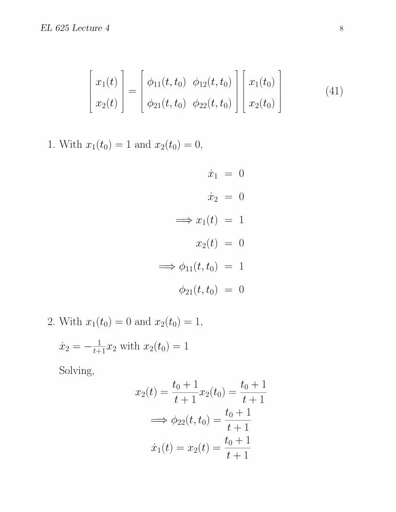
EL 625 Lecture 4 8

x1(t)

x2(t)

=

φ11(t, t0) φ12(t, t0)

φ21(t, t0) φ22(t, t0)

x1(t0)

x2(t0)

(41)

1. With x1(t0) = 1 and x2(t0) = 0,

x1 = 0

x2 = 0

=⇒ x1(t) = 1

x2(t) = 0

=⇒ φ11(t, t0) = 1

φ21(t, t0) = 0

2. With x1(t0) = 0 and x2(t0) = 1,

x2 = − 1t+1x2 with x2(t0) = 1

Solving,

x2(t) =t0 + 1t + 1

x2(t0) =t0 + 1t + 1

=⇒ φ22(t, t0) =t0 + 1t + 1

x1(t) = x2(t) =t0 + 1t + 1

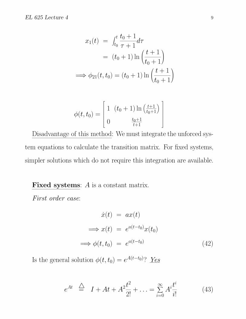
EL 625 Lecture 4 9

x1(t) =∫ t

t0

t0 + 1τ + 1

dτ

= (t0 + 1) ln

t + 1t0 + 1

=⇒ φ21(t, t0) = (t0 + 1) ln

t + 1t0 + 1

φ(t, t0) =

1 (t0 + 1) ln(

t+1t0+1

)

0 t0+1t+1

Disadvantage of this method: We must integrate the unforced sys-

tem equations to calculate the transition matrix. For fixed systems,

simpler solutions which do not require this integration are available.

Fixed systems: A is a constant matrix.

First order case:

x(t) = ax(t)

=⇒ x(t) = ea(t−t0)x(t0)

=⇒ φ(t, t0) = ea(t−t0) (42)

Is the general solution φ(t, t0) = eA(t−t0)? Yes

eAt =4 I + At + A2t2

2!+ . . . =

∞∑

i=0Ait

i

i!(43)

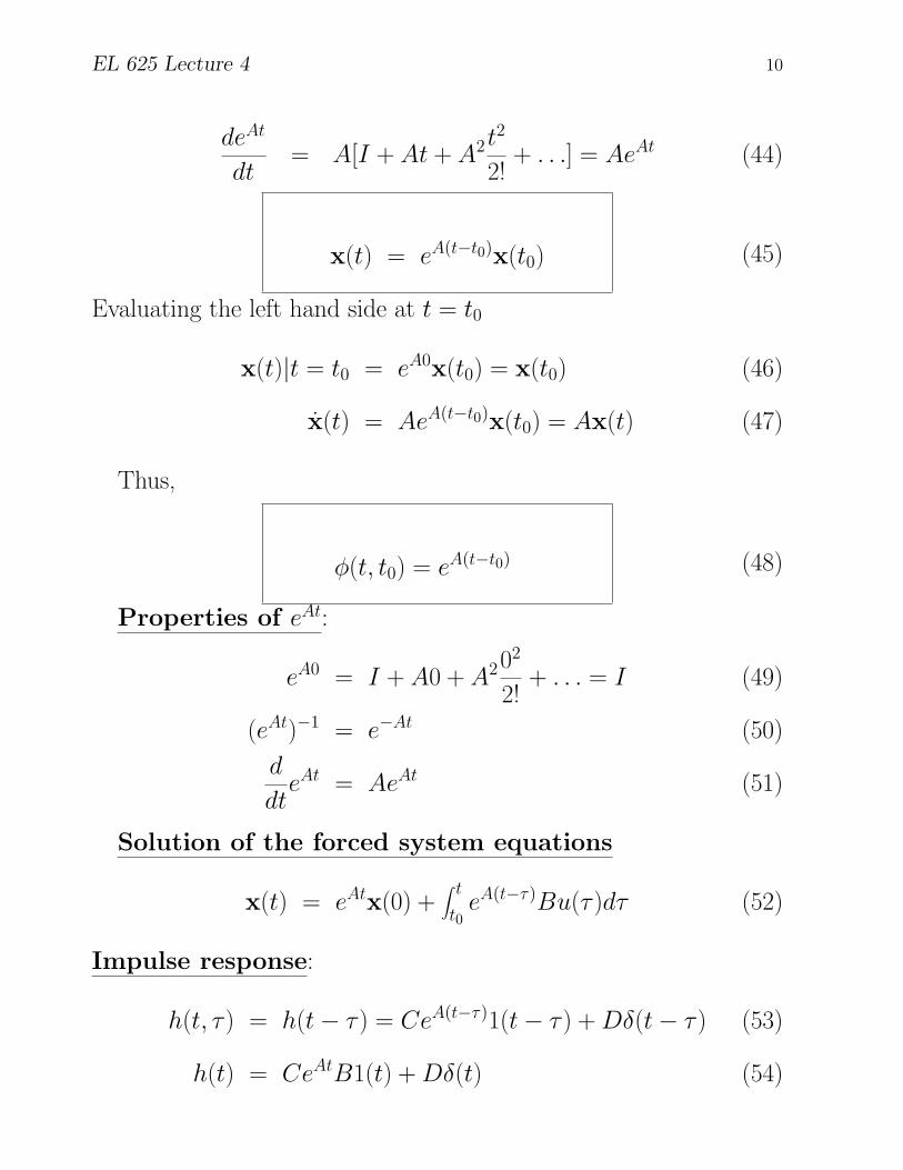
EL 625 Lecture 4 10

deAt

dt= A[I + At + A2t

2

2!+ . . .] = AeAt (44)

x(t) = eA(t−t0)x(t0) (45)

Evaluating the left hand side at t = t0

x(t)|t = t0 = eA0x(t0) = x(t0) (46)

x(t) = AeA(t−t0)x(t0) = Ax(t) (47)

Thus,

φ(t, t0) = eA(t−t0) (48)

Properties of eAt:

eA0 = I + A0 + A202

2!+ . . . = I (49)

(eAt)−1 = e−At (50)ddteAt = AeAt (51)

Solution of the forced system equations

x(t) = eAtx(0) +∫ t

t0eA(t−τ)Bu(τ )dτ (52)

Impulse response:

h(t, τ ) = h(t− τ ) = CeA(t−τ)1(t− τ ) +Dδ(t− τ ) (53)

h(t) = CeAtB1(t) + Dδ(t) (54)

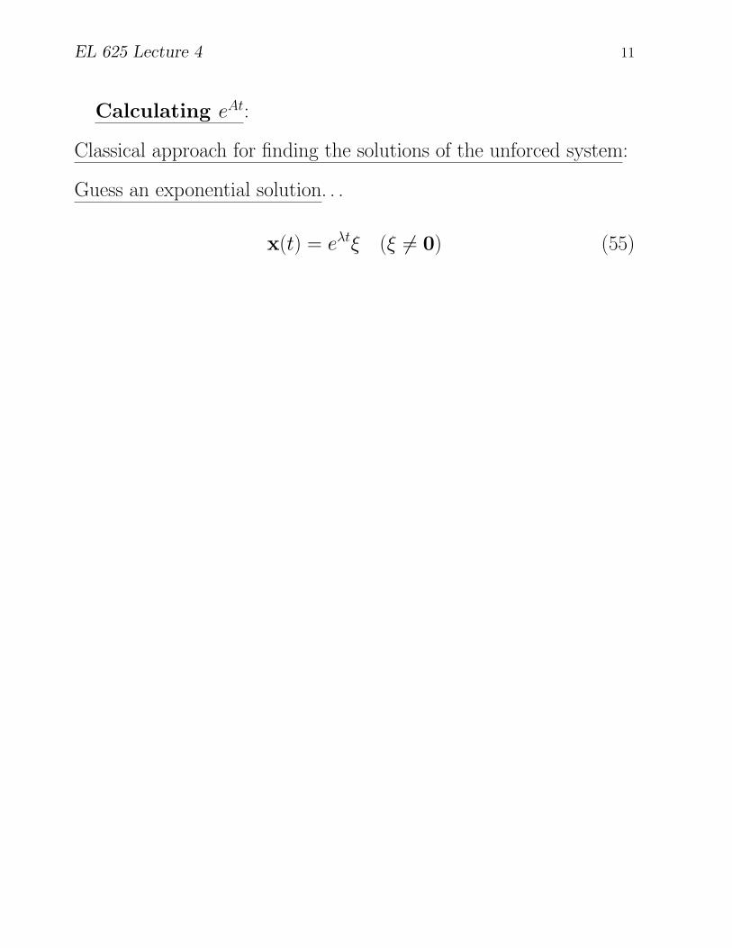
EL 625 Lecture 4 11

Calculating eAt:

Classical approach for finding the solutions of the unforced system:

Guess an exponential solution. . .

x(t) = eλtξ (ξ 6= 0) (55)

EL 625 Lecture 4 12

x(t) = λeλtξ

A(t)x(t) = λeλtξ

=⇒ Aeλtξ = λeλtξ

λξ = Aξ (56)

This is the ‘eigenvalue’ problem.

λ −→ eigenvalue

ξ −→ eigenvector (ξ 6= 0)

(λI − A)ξ = 0

det[λI − A] = 0 (57)

‘characteristic equation’ of the matrix A

p(λ) =4 det[λI − A] : an nth degree polynomial in λ, called the

characteristic polynomial.

EL 625 Lecture 4 13

Characteristic equation, p(λ) = 0 has n solutions,

the eigenvalues,λ1, λ2, . . . , λn −→ not necessarily distinct

For each eigenvalue, associated eigenvector equation:

[λiI − A]ξi = 0 (58)

has a nontrivial solution, ξi

Useful theorems from matrix theory:

1. Eigen vectors corresponding to distinct eigen values are linearly

independent.

Reminder: Vectors v1, v2, . . . vn are linearly independent if ∑ni=1 αivi =

0 =⇒ αi = 0∀i = 1, 2, ...n. In the figure below, v1 and v2 are

linearly independent. But, v1 and v3 are linearly dependent.

-

6

0

x

y�������

��

��

��

�������������

v1

v3

v2

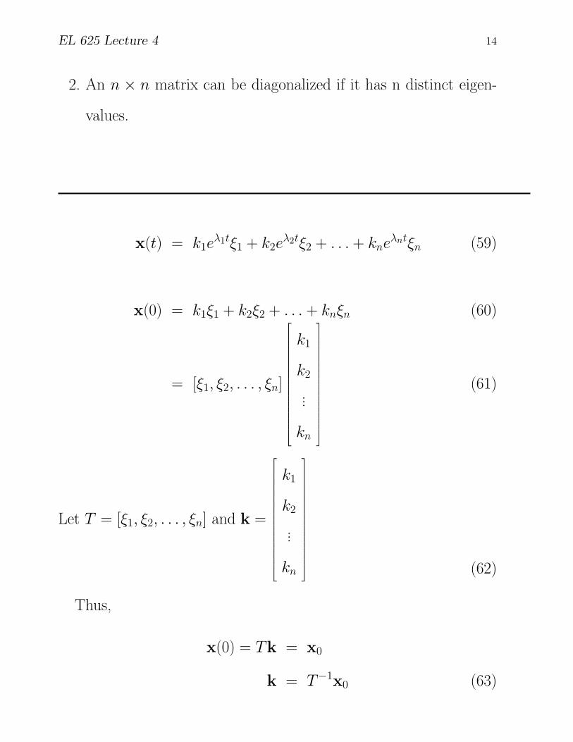
EL 625 Lecture 4 14

2. An n × n matrix can be diagonalized if it has n distinct eigen-

values.

x(t) = k1eλ1tξ1 + k2eλ2tξ2 + . . . + kneλntξn (59)

x(0) = k1ξ1 + k2ξ2 + . . . + knξn (60)

= [ξ1, ξ2, . . . , ξn]

k1

k2

...

kn

(61)

Let T = [ξ1, ξ2, . . . , ξn] and k =

k1

k2

...

kn

(62)

Thus,

x(0) = Tk = x0

k = T−1x0 (63)

EL 625 Lecture 4 15

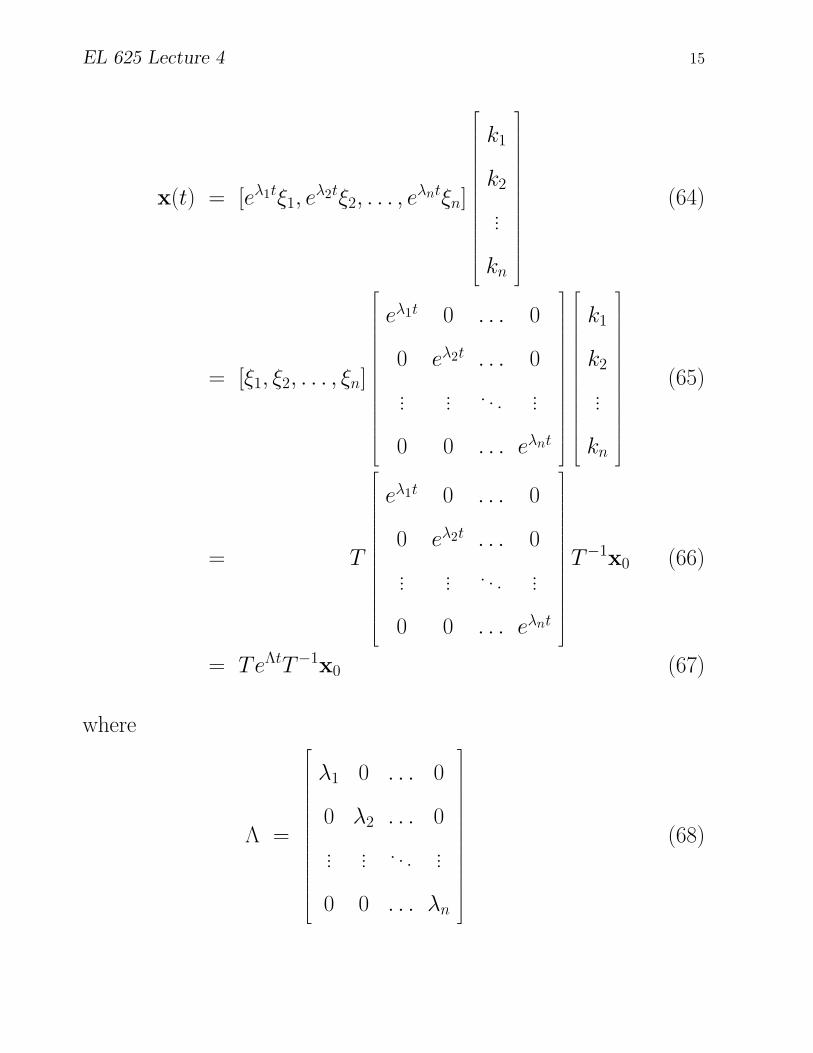
x(t) = [eλ1tξ1, eλ2tξ2, . . . , eλntξn]

k1

k2

...

kn

(64)

= [ξ1, ξ2, . . . , ξn]

eλ1t 0 . . . 0

0 eλ2t . . . 0... ... . . . ...

0 0 . . . eλnt

k1

k2

...

kn

(65)

= T

eλ1t 0 . . . 0

0 eλ2t . . . 0... ... . . . ...

0 0 . . . eλnt

T−1x0 (66)

= TeΛtT−1x0 (67)

where

Λ =

λ1 0 . . . 0

0 λ2 . . . 0... ... . . . ...

0 0 . . . λn

(68)

EL 625 Lecture 4 16

eΛt =

eλ1t 0 . . . 0

0 eλ2t . . . 0... ... . . . ...

0 0 . . . eλnt

(69)

Λi =

λi1 0 . . . 0

0 λi2 . . . 0... ... . . . ...

0 0 . . . λin

(70)

deΛt

dt=

λ1eλ1t 0 . . . 0

0 λ2eλ2t . . . 0... ... . . . ...

0 0 . . . λneλnt

= ΛeΛt (71)

x(t) = TeΛtT−1x0 (72)

x(t) = TΛeΛtT−1x0

= TΛT−1TeΛtT−1x0

= TΛT−1x(t)

= Ax(t) (73)

EL 625 Lecture 4 17

A = TΛT−1 (74)

T−1AT = Λ (75)

Thus, A is diagonalized by the similarity transformation, T .

If f (λ) is any function which can be expanded in a power series,

f (λ) =∞∑

i=0aiλi (76)

Define: f(A) = ∑∞i=0 aiA

i Thus,

f (A) =∞∑

i=0ai(TΛT−1)i (77)

=∞∑

i=0aiTΛiT−1 (78)

=∞∑

i=0aiT

λi1 0 . . . 0

0 λi2 . . . 0... ... . . . ...

0 0 . . . λin

T−1 (79)

= T

∑∞i=0 aiλ

i1 0 . . . 0

0 ∑∞i=0 aiλ

i2 . . . 0

... ... . . . ...

0 0 . . . ∑∞i=0 aiλ

in

︸ ︷︷ ︸

=4 f(Λ)

T−1 (80)

EL 625 Lecture 4 18

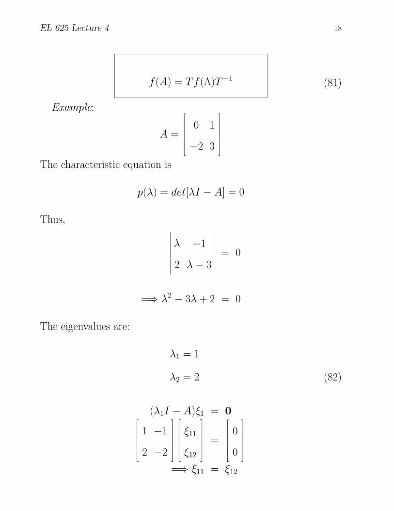
f(A) = Tf (Λ)T−1 (81)

Example:

A =

0 1

−2 3

The characteristic equation is

p(λ) = det[λI − A] = 0

Thus,

λ −1

2 λ− 3= 0

=⇒ λ2 − 3λ + 2 = 0

The eigenvalues are:

λ1 = 1

λ2 = 2 (82)

(λ1I − A)ξ1 = 0

1 −1

2 −2

ξ11

ξ12

=

0

0

=⇒ ξ11 = ξ12

EL 625 Lecture 4 19

Thus, the first eigenvector is

ξ1 =

1

1

(83)

(λ2I − A)ξ2 = 0

2 −1

2 −1

ξ21

ξ22

=

0

0

=⇒ ξ22 = 2ξ21

Thus, the second eigenvector is

ξ2 =

1

2

(84)

T = [ξ1, ξ2]

=

1 1

1 2

(85)

T−1 =

2 −1

−1 1

(86)

T−1AT =

1 0

0 2

= Λ (87)

EL 625 Lecture 4 20

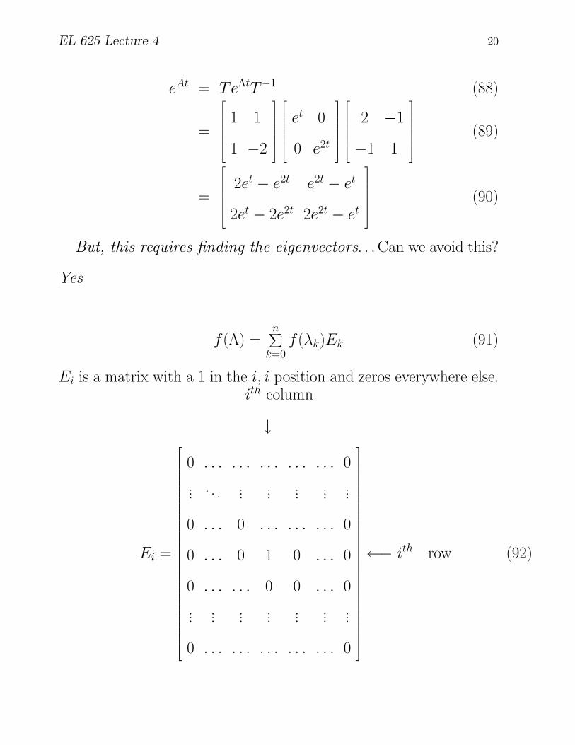
eAt = TeΛtT−1 (88)

=

1 1

1 −2

et 0

0 e2t

2 −1

−1 1

(89)

=

2et − e2t e2t − et

2et − 2e2t 2e2t − et

(90)

But, this requires finding the eigenvectors. . . Can we avoid this?

Yes

f (Λ) =n∑

k=0f (λk)Ek (91)

Ei is a matrix with a 1 in the i, i position and zeros everywhere else.ith column

↓

Ei =

0 . . . . . . . . . . . . . . . 0... . . . ... ... ... ... ...

0 . . . 0 . . . . . . . . . 0

0 . . . 0 1 0 . . . 0

0 . . . . . . 0 0 . . . 0... ... ... ... ... ... ...

0 . . . . . . . . . . . . . . . 0

←− ith row (92)

EL 625 Lecture 4 21

f (A) = Tf (Λ)T−1

=n∑

k=0f(λk)TEkT−1

=n∑

k=0f(λk)Zk0 (93)

where

Zk0 = TEkT−1 (94)

The matrices Zk0 are independent of the function f . Once

these matrices are evaluated, they can be used to find any function,

f(A).

Can we find Zk0 without finding T ? Yes

Method of Trial Functions: Choose a number of ‘trial func-

tions’ for which f(A) is easy to calculate and use these to calculate

Zk0.

Example:

A =

0 1

−2 3

The eigenvalues of this matrix are λ1 = 1 and λ2 = 2.

Using the method of trial functions, the calculation of the eigen-

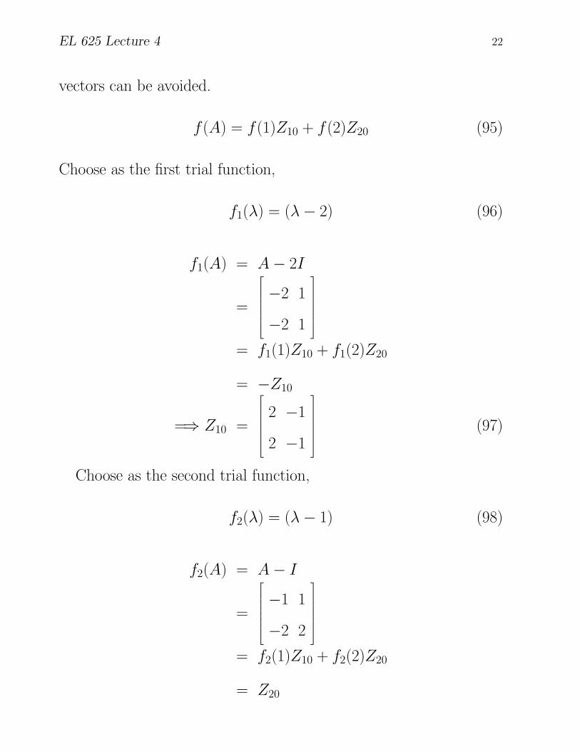
EL 625 Lecture 4 22

vectors can be avoided.

f (A) = f(1)Z10 + f (2)Z20 (95)

Choose as the first trial function,

f1(λ) = (λ− 2) (96)

f1(A) = A− 2I

=

−2 1

−2 1

= f1(1)Z10 + f1(2)Z20

= −Z10

=⇒ Z10 =

2 −1

2 −1

(97)

Choose as the second trial function,

f2(λ) = (λ− 1) (98)

f2(A) = A− I

=

−1 1

−2 2

= f2(1)Z10 + f2(2)Z20

= Z20

EL 625 Lecture 4 23

=⇒ Z20 =

−1 1

−2 2

(99)

Thus, for any function, f(λ),

f (A) = f(1)

2 −1

2 −1

+ f(2)

−1 1

−2 2

(100)

With f (λ) = eλt,

eAt = et

2 −1

2 −1

+ e2t

−1 1

−2 2

(101)

=

2et − e2t e2t − et

2et − 2e2t 2e2t − et

(102)

In general, if A has n distinct eigenvalues, λ1, λ2, . . . , λn, choose

as the kth trial function,

fk(λ) =n∏

i = 1

i 6= k

(λ− λi) (103)

fk(λj) =

0 for j 6= kn∏

i = 1i 6= k

(λk − λi) for j = k (104)

Zk0 =fk(A)fk(λk)

(105)

EL 625 Lecture 4 24

(106)

=

n∏

i = 1i 6= k

(A− λiI)

n∏

i = 1i 6= k

(λk − λi)(107)

(108)

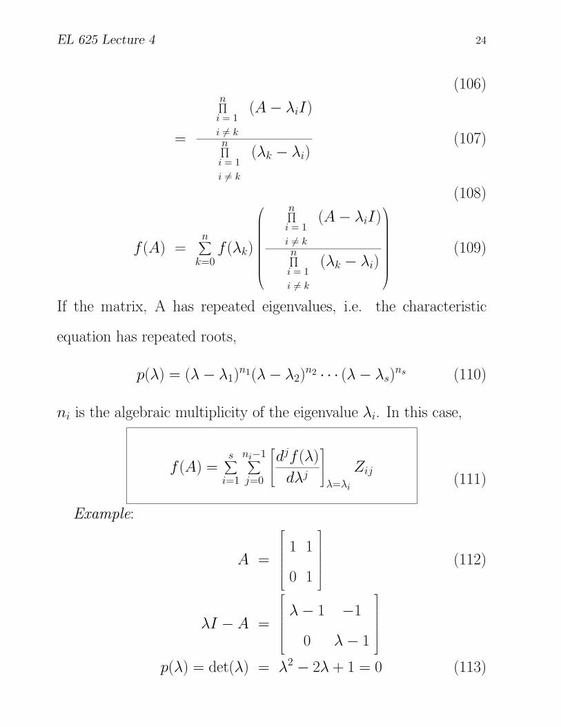
f (A) =n∑

k=0f (λk)

n∏

i = 1i 6= k

(A− λiI)

n∏

i = 1i 6= k

(λk − λi)

(109)

If the matrix, A has repeated eigenvalues, i.e. the characteristic

equation has repeated roots,

p(λ) = (λ− λ1)n1(λ− λ2)n2 · · · (λ− λs)ns (110)

ni is the algebraic multiplicity of the eigenvalue λi. In this case,

f (A) =s∑

i=1

ni−1∑

j=0

djf(λ)dλj

λ=λi

Zij(111)

Example:

A =

1 1

0 1

(112)

λI − A =

λ− 1 −1

0 λ− 1

p(λ) = det(λ) = λ2 − 2λ + 1 = 0 (113)

EL 625 Lecture 4 25

Thus, the matrix has a repeated eigen value at 1 i.e. λ1 = 1, λ2 = 1.

f (A) = f(1)Z10 + f ′(1)Z11 (114)

Choosing

f1(λ) = (λ− 1) (115)

f1(A) = A− I

=

0 1

0 0

= f1(1)Z10 + f ′1(λ)|λ=1Z11

= Z11

=⇒ Z11 =

0 1

0 0

(116)

Choosing,

f2(λ) = λ (117)

f2(A) = A

= f2(1)Z10 + f ′1(λ)|λ=1Z11

= Z10 + Z11

=⇒ Z10 = A− Z11

=

1 1

0 1

−

0 1

0 0

EL 625 Lecture 4 26

=

1 0

0 1

(118)

Thus, for any function f (λ) (which is differentiable at 1),

f (A) = f (1)

0 1

0 0

+ f ′(λ)|λ=1

1 0

0 1

(119)

With, f (λ) = eλt, f ′(λ)|λ=1 = teλt|λ=1 = tet

eAt = et

1 0

0 1

+ tet

0 1

0 0

(120)

=

et tet

0 et

(121)