Lecture: PolyhedralComputation,Spring2014 · Lecture: PolyhedralComputation,Spring2014 Komei Fukuda...

Lecture: Polyhedral Computation, Spring 2014

Komei Fukuda

Department of Mathematics, andInstitute of Theoretical Computer Science

ETH Zurich, Switzerland

February 18, 2014

i

Contents

1 Overview 1

2 Integers, Linear Equations and Complexity 32.1 Sizes of Rational Numbers . . . . . . . . . . . . . . . . . . . . . . . . . . . . 32.2 Linear Equations and Gaussian Elimination . . . . . . . . . . . . . . . . . . 32.3 Computing the GCD . . . . . . . . . . . . . . . . . . . . . . . . . . . . . . . 52.4 Computing the Hermite Normal Form . . . . . . . . . . . . . . . . . . . . . . 62.5 Lattices and the Hermite Normal Form . . . . . . . . . . . . . . . . . . . . . 102.6 Dual Lattices . . . . . . . . . . . . . . . . . . . . . . . . . . . . . . . . . . . 12

3 Linear Inequalities, Convexity and Polyhedra 133.1 Systems of Linear Inequalities . . . . . . . . . . . . . . . . . . . . . . . . . . 133.2 The Fourier-Motzkin Elimination . . . . . . . . . . . . . . . . . . . . . . . . 133.3 LP Duality . . . . . . . . . . . . . . . . . . . . . . . . . . . . . . . . . . . . 153.4 Three Theorems on Convexity . . . . . . . . . . . . . . . . . . . . . . . . . . 183.5 Representations of Polyhedra . . . . . . . . . . . . . . . . . . . . . . . . . . 193.6 The Structure of Polyhedra . . . . . . . . . . . . . . . . . . . . . . . . . . . 213.7 Some Basic Polyhedra . . . . . . . . . . . . . . . . . . . . . . . . . . . . . . 24

4 Integer Hull and Complexity 254.1 Hilbert Basis . . . . . . . . . . . . . . . . . . . . . . . . . . . . . . . . . . . 264.2 The Structure of Integer Hull . . . . . . . . . . . . . . . . . . . . . . . . . . 274.3 Complexity of Mixed Integer Programming . . . . . . . . . . . . . . . . . . . 294.4 Further Results on Lattice Points in Polyhedra . . . . . . . . . . . . . . . . . 30

5 Duality of Polyhedra 315.1 Face Lattice . . . . . . . . . . . . . . . . . . . . . . . . . . . . . . . . . . . . 315.2 Active Sets and Face Representations . . . . . . . . . . . . . . . . . . . . . . 325.3 Duality of Cones . . . . . . . . . . . . . . . . . . . . . . . . . . . . . . . . . 335.4 Duality of Polytopes . . . . . . . . . . . . . . . . . . . . . . . . . . . . . . . 355.5 Examples of Dual Pairs . . . . . . . . . . . . . . . . . . . . . . . . . . . . . . 375.6 Simple and Simplicial Polyhedra . . . . . . . . . . . . . . . . . . . . . . . . . 395.7 Graphs and Dual Graphs . . . . . . . . . . . . . . . . . . . . . . . . . . . . . 39

6 Line Shellings and Euler’s Relation 406.1 Line Shelling . . . . . . . . . . . . . . . . . . . . . . . . . . . . . . . . . . . 406.2 Cell Complexes and Visible Hemispheres . . . . . . . . . . . . . . . . . . . . 436.3 Many Different Line Shellings . . . . . . . . . . . . . . . . . . . . . . . . . . 45

7 McMullen’s Upper Bound Theorem 467.1 Cyclic Polytops and the Upper Bound Theorem . . . . . . . . . . . . . . . . 467.2 Simple Polytopes and h-vectors . . . . . . . . . . . . . . . . . . . . . . . . . 47

ii

8 Basic Computations with Polyhedra 528.1 Single H-Redundancy Checking . . . . . . . . . . . . . . . . . . . . . . . . . 538.2 H-Redundancy Romoval . . . . . . . . . . . . . . . . . . . . . . . . . . . . . 548.3 Computing H-Dimension . . . . . . . . . . . . . . . . . . . . . . . . . . . . . 568.4 Reducing the Nonhomogeneous Case to the Homogeneous Case . . . . . . . 58

9 Polyhedral Representation Conversion 599.1 Incremental Algorithms . . . . . . . . . . . . . . . . . . . . . . . . . . . . . . 599.2 Pivoting Algorithms . . . . . . . . . . . . . . . . . . . . . . . . . . . . . . . 639.3 Pivoting Algorithm vs Incremental Algorithm . . . . . . . . . . . . . . . . . 66

10 Hyperplane Arrangements and Point Configurations 6710.1 Cake Cutting . . . . . . . . . . . . . . . . . . . . . . . . . . . . . . . . . . . 6710.2 Arrangements of Hyperplanes and Zonotopes . . . . . . . . . . . . . . . . . . 7010.3 Face Counting Formulas for Arrangements and Zonotopes . . . . . . . . . . 7310.4 A Point Configuration and the Associated Arrangement . . . . . . . . . . . . 74

10.4.1 Application: Largest Feasible Subsystem . . . . . . . . . . . . . . . . 7510.4.2 Applications: Best Separation of Points by a Hyperplane . . . . . . . 75

11 Computing with Arrangements and Zonotopes 7611.1 Cell Generation for Arrangements . . . . . . . . . . . . . . . . . . . . . . . . 76

12 Minkowski Additions of Polytopes 7912.1 Complexity of Minskowski Sums of V-Polytopes . . . . . . . . . . . . . . . . 8112.2 Extension of a Zonotope Construction Algorithm . . . . . . . . . . . . . . . 82

13 Problem Reductions in Polyhedral Computation 8813.1 Hard Decision Problems in Polyhedral Computation . . . . . . . . . . . . . . 8813.2 Hard Enumeration Problems in Polyhedral Computation . . . . . . . . . . . 91

14 Evolutions and Applications of Polyhedral Computation 92

15 Literatures and Software 95

iii

IP (Fukuda) v.2014-02-18 1

1 Overview

Polyhedral computation deals with various computational problems associated with convexpolyhedra in general dimension. Typical problems include the representation conversionproblem (between halfspace and generator representations), the redundancy removal fromrepresentations, the construction of hyperplane arrangements and zonotopes, the Minkowskiaddition of convex polytopes, etc.

In this lecture, we study basic and advanced techniques for polyhedral computation ingeneral dimension. We review some classical results on convexity and convex polyhedrasuch as polyhedral duality, Euler’s relation, shellability, McMullen’s upper bound theorem,the Minkowski-Weyl theorem, face counting formulas for arrangements. Our main goal isto investigate fundamental problems in polyhedral computation from both the complexitytheory and the viewpoint of algorithmic design. Optimization methods, in particular, linearprogramming algorithms, will be used as essential building blocks of advanced algorithmsin polyhedral computation. Various research problems, both theoretical and algorithmic,in polyhedral computation will be presented. The lecture consist of the following sectionswhich are ordered in a way that the reader can follow naturally from top to bottom.

Lectures

1. Introduction to Polyhedral Computation

2. Integers, Linear Equations and Complexity

3. Linear Inequalities, Convexity and Polyhedra

4. Integer Hull and Complexity

5. Duality of Polyhedra

6. Line Shellings and Euler’s Relation

7. McMullen’s Upper Bound Theorem

8. Basic Computations with Polyhedra (Redundancy, Linearity and Dimension)

9. Polyhedral Representation Conversion

10. Hyperplane Arrangements and Point Configurations

11. Computing with Arrangements and Zonotopes

12. Minkowski Additions of Polytopes

13. Problem Reductions in Polyhedral Computation

14. * Voronoi Diagarams and Delaunay Triangulations

15. * Diophantine Approximation and Lattice Reduction

IP (Fukuda) v.2014-02-18 2

16. * Counting Lattice Points in Polyhedra

17. * Combinatorial Framework for Polyhedral Computation

18. Evolutions and Applications of Polyhedral Computation

19. Literatures and Software

(* planned.)

Case Studies

Matching Polytopes, Zonotopes and Hyperplane Arrangements, Bimatrix Games, OrderPolytopes, Cyclic Polytopes, etc. Note that this part is not yet integrated into the main text.See the supplementary notes, “Case Study on Polytopes (for Polyhedral Computation).”

IP (Fukuda) v.2014-02-18 3

2 Integers, Linear Equations and Complexity

2.1 Sizes of Rational Numbers

Whenever we evaluate the complexity of an algorithm, we use the binary encoding lengthof input data as input size and we bound the number of arithmetic operations necessaryto solve the worst-case problem instance of the same input size. Also, in order to claim apolynomial complexity, it is not enough that the number of required arithmetic operationsis bounded by a polynomial function in the input size, but also, the largest size of numbersgenerated by the algorithm must be bounded by a polynomial function in the input size.Here we formally define the sizes of a rational number, a rational vector and a rationalmatrix.

Let r = p/q be a rational number with canonical (i.e. relatively prime) representationwith p ∈ Z and q ∈ N. We define the binary encoding size of r as

size(r) := 1 + ⌈log2(|p|+ 1)⌉+ ⌈log2(q + 1)⌉. (2.1)

The binary encoding size of a rational vector v ∈ Qn and that of a rational matrix A ∈ Qm×n

are defined by

size(v) := n+n∑

j=1

size(vi), (2.2)

size(A) := mn+

m∑

i=1

n∑

j=1

size(aij). (2.3)

Exercise 2.1 For any two rational numbers r and s, show that

size(r × s) ≤ size(r) + size(s),

size(r + s) ≤ 2(size(r) + size(s)).

Can one replace the constant 2 by 1 in the second inequality?

2.2 Linear Equations and Gaussian Elimination

Theorem 2.1 Let A be a rational square matrix. Then the size of its determinant is poly-nomially bounded, and more specifically, size(det(A)) < 2 size(A).

Proof. Let p/q be the canonical representation of det(A), let pij/qij denote that of eachentry aij of A, and let δ denote size(A).

First, we observe

q ≤∏

i,j

qij < 2δ−1, (2.4)

where the last inequality can be verified by taking log2 of the both sides. By the definitionof determinant, we have

| det(A)| ≤∏

i,j

(|pij |+ 1). (2.5)

IP (Fukuda) v.2014-02-18 4

Combining (2.4) and (2.5),

|p| = | det(A)|q ≤∏

i,j

(|pij|+ 1)qij < 2δ−1, (2.6)

where the last inequality again is easily verifiable by taking log2 of both sides. Then itfollows from (2.4) and (2.6) that

size(det(A)) = 1 + ⌈log2(|p|+ 1)⌉+ ⌈log2(q + 1)⌉ ≤ 1 + (δ − 1) + (δ − 1) < 2δ. (2.7)

Corollary 2.2 Let A be a rational square matrix. Then the size of its inverse is polynomiallybounded by its size size(A).

Corollary 2.3 If Ax = b, a system of rational linear equations, has a solution, it has onepolynomially bounded by the sizes of [A, b].

Here is a theorem due to Jack Edmonds (1967).

Theorem 2.4 Let Ax = b be a system of rational linear equations. Then, there is apolynomial-time algorithm (based on the Gaussian or the Gauss-Jordan elimination) to findeither a solution x or a certificate of infeasibility, namely, λ such that λTA = 0 and λT b 6= 0.

Proof. Let ∆ be the size of the matrix [A, b]. We need to show that the size of any numberappearing in the Gaussian elimination is polynomially bounded by the size of input. Here weuse the Gauss-Jordan elimination without normalization. Let A be the matrix after applyingit for k times, that is, we have (after applying possible row and column permutations),

A =

1 · · · k s1 a11 0 · · · 0... 0

. . . 0k 0 · · · 0 akk

0 · · · 0

r 0. . . 0 ars

0 · · · 0

. (2.8)

Since we do not apply any normalization to nonzero diagonals, we have aii = aii 6= 0 for alli = 1, . . . , k. Let K = 1, . . . , k. We need to evaluate the sizes of all entries ars with s > k.For r > k, one can easily see

ars =det(AK∪r,K∪s)

det(AK,K)=

det(AK∪r,K∪s)

det(AK,K), (2.9)

where the last equation is valid because the elementary row operation without normalizationdoes not change the value of the determinant of any submatrix of A containing K as rowindices. It follows that size(ars) < 4∆. A similar argument yields size(ars) < 5∆ when r ≤ k.The same bounds for the size of the converted right hand side br follow exactly the same

IP (Fukuda) v.2014-02-18 5

way. When the system has a solution, there is one defined by xi = bi/aii for i = 1, . . . , kand xj = 0 for j > k, at the last step k of the algorithm. Clearly, the size of this solution is

polynomially bounded. When the system has no solution, there is a totally zero row Ar andbr 6= 0. It is left for the reader to find an efficient way to find a succinct certificate λ.

Exercise 2.2 Assuming that A, b are integer, revise the Gauss-Jordan algorithm so that itpreserves the integrality of intermediate matrices and is still polynomial. (Hint: each rowcan be scaled properly.)

2.3 Computing the GCD

For given two positive integers a and b, the following iterative procedure finds the greatestcommon divisor (GCD):

procedure EuclideanAlgorithm(a, b);begin

if a < b then swap a and b;while b 6= 0 dobegin

a := a− ⌊a/b⌋ × b;swap a and b;

end;output a;

end.

Note that the algorithm works not only for integers but rational a and b.

Exercise 2.3 Apply the algorithm to a = 212 and b = 288.

Exercise 2.4 Explain why it is a correct algorithm for GCD. Analyze the complexity of thealgorithm in terms of the sizes of inputs a and b. How can one extend the algorithm to workwith k positive integers?

This algorithm does a little more than computing the GCD. By looking at the matrixoperations associated with this, we will see that the algorithm does much more. Let’s lookat the two operations the algorithm uses in terms of matrices:

[a, b

] [0 11 0

]=[b, a

](2.10)

[a, b

] [ 1 0−⌊a/b⌋ , 1

]=[a− ⌊a/b⌋ × b, b

]. (2.11)

It is important to note that the two elementary transformation matrices[0 11 0

](Swapping),

[1 0

−⌊a/b⌋ , 1

](Remainder) (2.12)

IP (Fukuda) v.2014-02-18 6

are integer matrices and have determinant equal to +1 or −1. This means that the trans-formations preserve the existence of an integer solution to the following linear equation:

[a, b

] [xy

]= c (i.e., ax+ by = c). (2.13)

Let T ∈ Z2×2 be the product of all transformation matrices occurred during the Euclideanalgorithm applied to a and b. This means that | detT | = 1 and

[a, b

]T =

[a′, 0

], (2.14)

where a′ is the output of the Euclidean algorithm and thus GCD(a, b).Now, we see how the algorithm finds the general solution to the linear diophantine equa-

tion:

find

[xy

]∈ Z2 satisfying

[a, b

] [xy

]= c. (2.15)

Once the transformation matrix T is computed, the rest is rather straightforward. Since Tis integral and has determinant −1 or 1, the following equivalence follows.

⟨∃

[xy

]∈ Z2 :

[a, b

] [xy

]= c

⟩⇔

⟨∃

[x′

y′

]∈ Z2 :

[a, b

]T

[x′

y′

]= c

⟩

⇔

⟨∃

[x′

y′

]∈ Z2 :

[a′, 0

] [x′

y′

]= c

⟩⇔ 〈 a′|c (a′ divides c)〉 .

Finally, when a′|c, let x′ := c/a′ and y′ be any integer. Then,

[xy

]:= T

[x′

y′

]= T

[c/a′

y′

](2.16)

with y′ ∈ Z is the general solution to the diophantine equation (2.15).

2.4 Computing the Hermite Normal Form

By extending the Euclidean algorithm (in matrix form) to a system of linear equations inseveral integer variables, we obtain a procedure to solve the linear diophantine problem:

find x ∈ Zn satisfying Ax = b, (2.17)

where A ∈ Zm×n and b ∈ Zm are given. We assume that A is full row rank. (Otherwise,one can either reduce the problem to satisfy this condition or show that there is no x ∈ Rn

satisfying Ax = b. How?)Note that a seemingly more general problem of rational inputs A and b can be easily

scaled to an equivalent problem with integer inputs.

Theorem 2.5 There is a finite algorithm to find an n×n integer matrix T with | detT | = 1such that A T is of form [B 0], where B = [bij ] is an m×m nonnegative nonsingular lower-triangular integer matrix with bii > 0 and bij < bii for all i = 1, . . . , m and j = 1, . . . , i− 1.

IP (Fukuda) v.2014-02-18 7

This matrix [B 0] is known as the Hermite normal form, and it will be shown that it isunique.

Corollary 2.6 The linear diophantine problem (2.17) has no solution x if and only if thereis z ∈ Qm such that zTA is integer and zT b is fractional.

Proof. The “if” part is trivial. To prove the “only if” part, we assume that ∄x ∈ Zn :A x = b. Let T be the integer matrix given by Theorem 2.5. Because | detT | = 1, we havethe following equivalence:

〈∄x ∈ Zn : A x = b〉 ⇔ 〈∄x′ ∈ Zn : A T x′ = b〉 ⇔ 〈∄x′ ∈ Zn : [B 0] x′ = b〉

⇔⟨B−1b is not integer

⟩.

Since B−1b is not integer, there is a row vector zT of B−1 such that zT b is fractional. SinceB−1A T = [I 0], we know that B−1A = [I 0]T−1 and it is an integer matrix as | det T | = 1.This implies that zTA is integer. This completes the proof.

As for the single diophantine equation, one can write the general solution to the lineardiophantine problem (2.17).

Corollary 2.7 Let A ∈ Qm×n be a matrix of full row rank, b ∈ Qm, and A T = [B 0] be anHermite normal form of A. Then the following statements hold.

(a) The linear diophantine problem (2.17) has a solution if and only if B−1b is integer.

(b) If B−1b is integer, then the general solution x to (2.17) can be written as

x =T

[B−1bz

], (2.18)

for any z ∈ Zn−m.

Now, we are going to prove the main theorem, Theorem 2.5.

Proof. (of Theorem 2.5). Extending the operations we used in (2.12), our proof ofTheorem 2.5 involves three elementary matrix (column) operations on A:

(c-0) multiplying a column of A by −1;

(c-1) swapping the positions of two columns of A;

(c-2) adding an integer multiple of a column to another column of A.

Both (c-1) and (c-2) were already used and (c-0) is merely to deal with negative entries whichare allowed inA. Each operation can be written in formA T , where T is a unimodularmatrix,i.e., an integer matrix of determinant equal to −1 or 1.

The algorithm operates on the first row, the second and to the last row. We may assumethat we have already transformed the first k(≥ 0) rows properly, namely, we have a sequenceof matrices T1, T2,..., Ts such that T = T1T2 · · ·Ts and

Ak := A T =

[B′ 0C A′

](2.19)

IP (Fukuda) v.2014-02-18 8

where B′ is a k × k matrix which is already in the form required for the final B, namely, itis a nonnegative nonsigular lower-triangular integer matrix with b′ii > 0 and b′ij < b′ii for alli = 1, . . . , k and j = 1, . . . , i− 1. Now we process the kth row of Ak, and essentially the firstrow of A′. The first row of A′ contains n− k integers and the rest is written by A′′:

A′ =

[a′11, a

′12, . . . , a

′1(n−k)

A′′

](2.20)

Now we apply the Euclidean algorithm to find the GCD, say α, of the n − k integers. Forthis, we first use (c-0) operations to make the numbers all nonnegative. Then remainingoperations are straightforward with (c-1) and (c-2) to convert the first row to [α, 0, 0, . . . , 0].This in the form of the whole matrix Ak looks like (for some T ′),

Ak T′ =

B′ 0

Cα, 0, 0, . . . , 0

A′′′

. (2.21)

Note that α is strictly positive because of the full row rank assumption. Finally, we canreduce the entries in the first row of C by adding some integer multiples of α in the (k+1)stcolumn (for some T ′′) as

Ak T′ T ′′ =

B′ 0c′11, . . . , c

′1k α, 0, 0, . . . , 0

C ′′ A′′′

, (2.22)

so that all entries c′11, . . . , c′1k are smaller than α. Now we have made the principal (k+1)×

(k + 1) matrix in the form of the final B. This completes the proof.While the algorithm is finite, it is not clear how good this is. It has been observed that

the largest size of numbers appearing during the course of the algorithm grows rapidly. Thereare ways to make the procedure polynomial. We will discuss this issue later.

Example 2.1 The following small example is simple enough to calculate by hand.

A =

[−8 10 −4−4 −2 8

],

A1 =

[2 0 014 20 −36

],

A2 = [B 0] =

[2 0 02 4 0

].

The transformation matrix T with A2 = A T is

T =

6 −2 97 −2 105 −1 7

.

IP (Fukuda) v.2014-02-18 9

Example 2.2 The following small example (randomly generated) shows how numbers growrapidly. Of course, this example is not meant to be computed by hand.

A =

−100 −32 140 168 14768 −16 −125 168 7

−12 −28 −50 147 −133−60 64 −65 28 28

,

A1 =

1 0 0 0 0−523 944 159 320 1976−115 604 54 151 388976 −2080 −565 −156 −3652

,

A2 =

1 0 0 0 00 1 0 0 0

−1489619 −2848 −495 5739 −1722−37305137 −71331 −6180 143636 −29988

,

A3 =

1 0 0 0 00 1 0 0 01 2 3 0 0

−299296004657 −572624931 −602688 309680 1400700

,

A4 = [B 0] =

1 0 0 0 00 1 0 0 01 2 3 0 043 129 12 140 0

.

The transformation matrix T with A4 = A T is

T =

−807814365429333 −1545542680854 −1626716396 −377867 1101240−1448925874428057 −2772142804282 −2917738997 −677754 1975225−731120268289411 −1398808473625 −1472275536 −341992 996688−365381147997122 −699061793372 −735777339 −170912 498100248937455097979 476277073276 501291704 116444 −339360

.

Observation 2.8 In the example above, the numbers appearing during the course of the al-gorithm seem to grow. This is a fact commonly observed. Yet, it is not known if our algorithmis exponential. There are ways to modify the algorithm so that it runs in polynomial-time.

Exercise 2.5 Write a computer program to compute a Hermite normal form of any integermatrix A of full row rank. For this, one needs to use an environment where infinite precisioninteger arithmetic is supported, e.g., C/C++ with GNU gmp, Mathematica, Maple, andSage.

IP (Fukuda) v.2014-02-18 10

2.5 Lattices and the Hermite Normal Form

There is a close relationship between the Hermite normal form of a matrix A ∈ Qm×n andthe lattice generated by (the columns of) A. Recall that the lattice L(A) generated by A isdefined by

L(A) = y : y = Ax, x ∈ Zn. (2.23)

The lattice L(A) is full dimensional if it spans the whole space Rm, or equivalently, A is fullrow rank.

Lemma 2.9 Let A be rational matrix of full row rank with Hermite normal form [B 0]Then, L(A) = L([B 0]).

Proof. This follows directly from the fact that A T = [B 0] for some unimodular matrixT .

Theorem 2.10 Let A and A′ be rational matrices of full row rank with Hermite normalforms [B 0] and [B′ 0], respectively. Then the matrices A and A′ generate the same lattice(i.e. L(A) = L(A′)) if and only if B = B′.

Proof. Clearly, the sufficiency is clear: if B = B′, L(A) = L(A′).Assume that L := L(A) = L(A′). Then, by Lemma 2.9, L = L(B) = L(B′). Now we

show that the kth columns B·k and B′·k are equal for k = 1, . . . , n. First, observe that B·k

and B′·k are in L with the property (*) that the first (k − 1) components are all zero and

the kth component is positive. Because B is in Hermite normal form, it follows that B·k isa vector in L satisfying (*) with its kth component being smallest possible. Since the samething can be said about B′

·k, bkk = b′kk for k = 1, . . . , n. In addition, because B is in Hermitenormal form, B·k is a lexicographically smallest vector of nonnegative components satisfying(*), and so is B′

·k. Such a vector is unique, and thus B·k = B′·k.

Corollary 2.11 Every rational matrix of full row rank has a unique Hermite normal form.

A basis of a full dimensional lattice L(A) is a nonsingular matrix B such that L(A) =L(B). A direct consequence of Theorem 2.5 is

Corollary 2.12 Every rational matrix of full row rank has a basis.

Exercise 2.6 Let A be a rational matrix of full row rank, let B be a bases of L(A) andlet B′ be a nonsingular n × n matrix whose column vectors are points in L(A). Show thefollowing statements are valid:

(a) | det(B)| ≤ | det(B′)|.

(b) B′ is a basis of L(A) if and only if | det(B)| = | det(B′)|.

Using the fact (a) above, we show that the size of the Hermite normal form is small.

IP (Fukuda) v.2014-02-18 11

Theorem 2.13 The size of the Hermite normal form of a rational matrix A of full row rankis polynomially bounded by size(A).

Proof. Let [B 0] be the Hermite normal form of A, and let B′ be any basis (i.e. nonsingu-lar m×m submatrix) of A (which is not necessarily a basis of L(A)). First of all, det(B) > 0.By Exercise 2.6 (a), we have det(B) ≤ | det(B′)|. By Theorem 2.1, this inequality impliesthat the size of det(B) is polynomially bounded by size(A).

Since B is lower triangular, det(B) is the product of diagonal entries bii, (i = 1, ..., n). Itfollows that the size of each entry bii is less than the size of det(B), and thus is polynomiallybounded by size(A). Since B is in Hermite normal form, each nondiagonal entry bij is lessthan or equal to bii and has the same property.

The theorem above suggests that the Hermite Normal Form might be computable inpolynomial time. In fact, there are methods to control the largest size of numbers generatedduring the course of the algorithm given in the previous section.

One such algorithm is as follows. First of all, a given matrix A of full row rank, is enlargedto

A :=

M 0 · · · 0

A 0. . . 0

0 · · · 0 M

, (2.24)

where M is set to be the positive integer | det(B′)| for an arbitrarily chosen basis B′ of A.The first observation is that this new matrix generates the same lattice as A.

Exercise 2.7 Show that L(A) = L(A).

Thus, computing the Hermite normal form of A is equivalent to that of A. Now, since wehave the added columns, it is possible to reduce the entries appearing in the first n columnsby adding proper multiples of the last m columns, so that all entries are nonnegative andat most M . This reduction should be applied before the Euclidean algorithm is applied toeach row. Since size(M) is polynomially bounded by size(A), one can control the numberof arithmetic operations and the size of numbers appearing in the application of Euclideanalgorithm applied to each row of A.

The sources of the ideas and more detailed discussion can be found in Shrijver’s book[47, Section 5.3]. One important consequence of Theorem 2.13 , Corollary 2.3 and Theorem2.4 is the following.

Corollary 2.14 For any rational matrix A of full row rank, there is a transformation matrixT such that AT is the Hermite normal form of A and size(T ) is polynomially bounded by thesize of A. Furthermore, such a matrix can be computed in polynomial time.

IP (Fukuda) v.2014-02-18 12

2.6 Dual Lattices

For a lattice L in Rm, its dual lattice L∗ is defined by

L∗ := y ∈ Qm : yTz ∈ Z, ∀z ∈ L. (2.25)

If L is generated by a matrix A,

L∗ = (L(A))∗ = y ∈ Qm : yTA ∈ Zn. (2.26)

In terms of the Hermite normal form [B 0] of A (assuming A is full row rank), the duallattice is generated by the transpose (and the rows) of B−1, that is,

L∗ = L((B−1)T ). (2.27)

Why is it so? To see that, set L′ = L((B−1)T ) and we will show L′ = L∗. Since B−1B = Iand L is generated by (the columns of) B, each row of B−1 has an integer inner productwith any vector in L. This shows L′ ⊆ L∗. For the converse, take any vector y in L∗. LetsT = yTB. By definition of L∗, s ∈ Zm. Observing that yT = sTB−1, y is an integer linearcombination of the rows of B−1. This proves L′ ⊇ L∗ and completes the proof.

Example 2.3 Figure 2.1 left depicts the lattice generated by A =

[1 1−1 2

]. The Hermite

normal form is B =

[1 02 3

]and its inverse is B−1 =

[1 0−2

313

]. While the primal lattice L(A)

is generated by the columns of B, the dual lattice (L(A))∗ is generated by the rows of B−1.Figure 2.1 right depicts the dual lattices (partially) on the same scale.

-4 -2 2 4

-15

-10

-5

5

10

15

-4 -2 2 4

-15

-10

-5

5

10

15

Figure 2.1: Lattice L(A) and its Dual Lattice.

IP (Fukuda) v.2014-02-18 13

3 Linear Inequalities, Convexity and Polyhedra

3.1 Systems of Linear Inequalities

Consider a system of rational linear inequalities

Ax ≤ b, (3.1)

where A ∈ Qm×d and b ∈ Qm are given. The set

P = P (A, b) := x ∈ Rd : Ax ≤ b (3.2)

of solutions to the system is a subset of Rd, known as a convex polyhedron. It is in fact aconvex set: a subset C of Rd is said to be convex if the line segment [u, v] := x : x =αu+ (1− α)v, 0 ≤ α ≤ 1 between any two points u and v in C is entirely contained in C.A bounded convex polyhedron is called a convex polytope.

A point x is called an extreme point of a convex set C if x ∈ C and x is not on the linesegment between any two points u, v in C different from x. Unlike general convex sets, aconvex polyhedron P contains only a finite number of extreme points. This will be shownin a more general form in Theorem 3.14.

Below, the first two are centrally symmetric polytopes in R3, and the third one is ran-domly generated. One can interpret the third one as a bounded polyhedron (i.e. polytope)contained in the nonnegative orthant or as an unbounded polyhedron having only its non-negative orthant part drawn.

3.2 The Fourier-Motzkin Elimination

Consider a system (3.1) of m linear inequalities in n variables. Solving such a system meanseither to find a rational vector x satisfying the system or to detect inconsistency of thesystem. The latter can be proven by a certificate given by the well-known theorem of Gale:

Theorem 3.1 (Gale’s Theorem) For any A ∈ Rm×d and b ∈ Rm, exactly one of thefollowing statements holds:

(a) there exists x ∈ Rd such that Ax ≤ b;

(b) there exists z ∈ Rm such that z ≥ 0, zTA = 0 and zT b < 0.

IP (Fukuda) v.2014-02-18 14

It is easy to see that both statements cannot hold simultaneously as it would mean 0is less than or equal to some (strictly) negative number. Thus the nontrivial part of thetheorem is that one of (a) and (b) is always valid. There are several constructive proofs ofthe theorem.

Here we present an arguably simplest constructive proof due to Fourier and Motzkin.The main idea is to transform the system (3.1) to an equivalent system of the same formwith one less variables.

First we rewrite the system (3.1) by looking at the coefficients aid’s for the last variablexd. Let us define a partition of row indices into the three sets:

I+ := i | aid > 0, I− := i | aid < 0 and I0 := i | aid = 0.

The system (3.1) can be rewritten by solving each inequality with respect to xd:

xd ≤ fi(x′) ∀i ∈ I+

gj(x′) ≤ xd ∀j ∈ I−

hk(x′) ≤ 0 ∀k ∈ I0,

where x′ is the vector x with the last component eliminated, i.e. x′ = (x1, . . . , xd−1)T and

each functions fi, gj and hk denote some affine functions in d− 1 variables.It is not difficult to show (Exercise 3.1) that the system (3.1) is equivalent to the new

system in d− 1 variables:

gj(x′) ≤ fi(x

′) ∀(i, j) ∈ I+ × I−

hk(x′) ≤ 0 ∀k ∈ I0.

This system can thus be written as

A′x′ ≤ b′. (3.3)

Exercise 3.1 Prove the equivalence: Ax ≤ b ⇔ A′x′ ≤ b′.

No reason to stop here. Let’s continue to eliminate the variable xd−1, then xd−2 and soforth until all variables are eliminated. This generates a sequence of equivalent systems oflinear inequalities:

A(0)x(0) ≤ b(0) (This is the original system Ax ≤ b.)

m

A(1)x(1) ≤ b(1) (This is A′x′ ≤ b′ above.)

m

A(2)x(2) ≤ b(2)

m...

m

A(d)x(d) ≤ b(d),

where A(k)x(k) ≤ b(k) denotes the kth system where the last k variables have been eliminated.

IP (Fukuda) v.2014-02-18 15

Exercise 3.2 Show that the elimination step as a matrix transformation. More precisely,there is a matrix T (depending on A) such that the system A′x′ ≤ b′ is the same system asTAx ≤ Tb up to positive scaling. Note that the last column of the product TA is totallyzero and thus TAx does not involve the last variable xd.

By the exercise above, the last system A(d)x(d) ≤ b(d) can be now written as T (d)Ax ≤T (d)b. Of course, the left hand side T (d)Ax is a vector of zero’s.

Exercise 3.3 Prove Theorem 3.1 by using the matrix T (d).

Exercise 3.4 Prove the following forms of alternative theorem using Gale’s Theorem. Be-low, the statement is read as “exactly one of the two statements (a) or (b) holds.”

The Farkas Lemma

(a) ∃x : A x = b and x ≥ 0;

(b) ∃z : zTA ≥ 0 and zT b < 0.

Gordan’s Theorem

(a) ∃x : A x = 0 and x 0;

(b) ∃z : zTA > 0.

3.3 LP Duality

For a given A ∈ Rm×d, b ∈ Rm, c ∈ Rd, the linear programming problem (in canonical form)is

(P): max cTx =∑d

j=1 cj xj

subject to A x ≤ b∑d

j=1 aij xj ≤ bi, ∀i = 1, . . . , m

x ≥ 0. xj ≥ 0, ∀j = 1, . . . , d.

We often abbreviate a linear programming problem as an LP. A vector x satisfying all theconstraints Ax ≤ b and x ≥ 0 is called a feasible solution. An optimal solution is a feasiblesolution that attains the largest objective value. In the case of minimization problem, anoptimal solution attains the smallest value.

The set of feasible solutions x : Ax ≤ b, x ≥ 0 is called the feasible region. An LP iscalled feasible if the feasible region is not empty. An LP is called unbounded if the objectivefunction cTx is not bounded above (below for the minimization case) over the feasible region.

Geometrically, the feasible region is a convex polyhedron.

x3

x1

x2

x3

x1

x2

IP (Fukuda) v.2014-02-18 16

In general, maximizing or minimizing a linear function subject to a system of linear inequalityconstraints in d variables can be reduced to an optimization in the form above. Also, notethat no strict inequality constraint such as x1 > 0 is allowed in linear programming.

There are two fundamental theorems, the weak duality theorem and the strong dualitytheorem. To state these theorems, we need to define the dual problem

(D): min bT ysubject to ATy ≥ c

y ≥ 0

which is a linear programming problem itself. The original problem (P) is called the primalproblem when we need to distinguish it from the dual problem.

Theorem 3.2 (LP Weak Duality Theorem) For any feasible solution x for the primalproblem (P) and for any feasible solution y for the dual problem (D), cTx ≤ bTy.

Theorem 3.3 (LP Strong Duality Theorem) If both the primal problem (P) and thedual problem (D) are feasible, there exist a dual pair (x∗, y∗) of feasible solutions such thatcTx∗ = bTy∗. (By the previous theorem, they are both optimal.)

The first theorem is very easy to prove. Thus it may not be appropriate to call it atheorem, but since it is widely accepted to be so called. Let’s prove it.

Proof. (of the Weak Duality Theorem, Theorem 3.2) Let x and y be a dual pair of feasiblesolutions. Then,

cTx ≤ (ATy)Tx (because ATy ≥ c and x ≥ 0)

= yTAx

≤ yT b (because Ax ≤ b and y ≥ 0)

= bTy.

This completes the proof.Now, we are ready to prove the second theorem which is much harder to prove.

Proof. (of the Strong Duality Theorem, Theorem 3.3) Assume that both the primalproblem (P) and the dual problem (D) are feasible. We have to show that

∃(x, y) :Ax ≤ b, x ≥ 0

ATy ≥ c, y ≥ 0

cTx = bT y.

(3.4)

Now, we verify the statement (3.4) is always valid under the assumption.

IP (Fukuda) v.2014-02-18 17

(3.4) ⇔

⟨ ∃(x, y) : Ax ≤ b, x ≥ 0ATy ≥ c, y ≥ 0cTx ≥ bTy

⟩(by the Weak Duality)

⇔

⟨∃

[xy

]≥ 0 :

A 0−I 00 −AT

0 −I−cT bT

[xy

]≤

b0−c00

⟩

⇔

⟨6 ∃

stuvw

≥ 0 :

stuvw

T

A 0−I 00 −AT

0 −I−cT bT

= 0 and

stuvw

T

b0−c00

< 0

⟩(by Gale’s Thm)

⇔

⟨6 ∃

suw

≥ 0 : AT s ≥ cw,Au ≤ bw, bT s < cTu

⟩

⇔

⟨6 ∃

[su

]≥ 0 : AT s ≥ 0, Au ≤ 0, bT s < cTu

⟩(by the Weak Duality)

⇔⟨AT s ≥ 0, Au ≤ 0, s ≥ 0, u ≥ 0 ⇒ bT s ≥ cTu

⟩.

Now the last step of the proof is to show the last statement above is always true whichimplies the theorem. Assume

AT s ≥ 0, Au ≤ 0, s ≥ 0, u ≥ 0.

By the assumption, we have a dual pair (x, y) of feasible solutions. Thus, we have

bT s− cTu ≥ (Ax)T s− (ATy)Tu = xTAT s− yTAu ≥ 0− 0 = 0.

This completes the proof.

Theorem 3.4 (Complementary Slackness Conditions) For a dual pair (x, y) of feasi-ble solutions for (P) and (D), the following conditions are equivalent:

(a) both x and y are optimal solutions;

(b) cTx = bT y;

(c) yT (b− Ax) = 0 and xT (ATy − c) = 0.

(c’) yi(b−Ax)i = 0 for all i and xj(AT y − c)j = 0 for all j.

(c”) yi > 0 implies (b− Ax)i = 0, for all i andxj > 0 implies (ATy − c)j = 0, for all j.

Proof. Left to the reader.

Exercise 3.5 Write the Complementary Slackness Conditions (Theorem 3.4) for the LP ofform max cTx subject to Ax ≤ b and its dual LP, and prove the validity.

IP (Fukuda) v.2014-02-18 18

3.4 Three Theorems on Convexity

Before we discuss the theory of representations and combinatorial structure of convex poly-hedron, it is good to mention some basic facts about convexity.

For any subset S of Rd, the convex hull conv(S) of S is the intersection of all convex setscontaining S. Since the intersection of two convex sets is convex, it is the smallest convexset containing S.

Proposition 3.5 Let S be a subset Rd. Then

conv(S) = x : x =

k∑

i=1

λipi,

k∑

i=1

λi = 1, λi ≥ 0 ∀i = 1, . . . , k,

for some finite points p1, . . . , pk ∈ S.

(3.5)

Proof. Let the RHS of (3.5) be T . One has to show both inclusions conv(S) ⊇ T andconv(S) ⊆ T . Both inclusions are elementary and left to the reader.

One basic theorem on convexity is Caratheodory’s theorem, saying that the finitenesscondition on k in (3.5) can be much more restrictive, namely, k ≤ d+ 1.

Theorem 3.6 (Caratheodory’s Theorem) Let a point p be in the convex hull of a set Sof k points p1, . . . , pk in Rd. Then p is in the convex hull of at most d+ 1 points in S.

Proof. Left to the reader. Hint: When k ≥ d + 2, the points p1, . . . , pk are affinelydependent, i.e., there exist α1, . . . , αk not all zero such that

∑i αi = 0 and

∑i αipi = 0. Use

this to show that at least one point in S is unnecessary to represent x.

Here are two more basic theorems on convexity.

Theorem 3.7 (Radon’s Theorem) Let S be a subset of of Rd with |S| ≥ d+ 2. Then Scan be partitioned into two sets S1 and S2 so that conv(S1) ∩ conv(S2) 6= ∅.

S1S2

Proof. Since |S| ≥ d + 2, the points in S are affinely dependent. Use this fact to find anatural partition.

Theorem 3.8 (Helly’s Theorem) Let C1, C2, . . . , Ch be convex sets in Rd such that C1 ∩C2 ∩ · · · ∩ Ch = ∅. Then, there are at most d+ 1 of them whose intersection is empty.

IP (Fukuda) v.2014-02-18 19

C1

C4

C2

C3

Proof. (Clearly, the convexity assumption on Cj ’s is important as the theorem fails withonly one nonconvex Cj above.) Use induction on h. If h ≤ d + 1, the theorem is trivial.Assume that the theorem is true for h < k(≥ d+2) and prove (*) the theorem holds for h = k.Note that h ≥ d + 2. Suppose the statement (*) does not hold, namely, Sj := ∩j 6=iCj 6= ∅for all j = 1, . . . , h. Apply Radon’s theorem to get a contradiction.

3.5 Representations of Polyhedra

For a set v1, . . . , vk of vectors in Rd, define their cone (or nonnegative) hull as

cone(v1, . . . , vk) := x : x =∑

i

λivi, λi ≥ 0 ∀i = 1, . . . , k. (3.6)

For subsets P and Q of Rd, their Minkowski sum P +Q is defined as

P +Q := p+ q : p ∈ P and q ∈ Q. (3.7)

Theorem 3.9 (Minkowski-Weyl’s Theorem for Polyhedra) For P ⊆ Rd, the follow-ing statements are equivalent:

(a) P is a polyhedron, i.e., there exist A ∈ Rm×d and b ∈ Rm for some m such thatP = x : Ax ≤ b;

(b) P is finitely generated, i.e., there exist (finite) vectors vi’s and rj’s in Rd such thatP = conv(v1, . . . , vs) + cone(r1, . . . , rt).

The statement (b) above can be written in matrix form as follows. Here, 1 denotes avector of all 1s.

(b) P is finitely generated, i.e., there exist two matrices V ∈ Rd×s and R ∈ Rd×t for some sand t such that P = x : x = V µ+Rλ, µ ≥ 0, 1Tµ = 1, λ ≥ 0.

Theorem 3.9 actually consists of two theorems. The direction from (a) to (b) is Minkowski’sThoerem, while the reverse direction from (b) to (a) is Weyl’s Theorem.

When a polyhedron P is bounded (thus a polytope), the minimal representation consistsof all extreme points v1, . . ., vs and no rays. Another special case of b = 0 leads to ahomogeneous version of the theorem. It is a special case but it is actually as powerful as thenonhomogeneous version above (Exercise 3.6).

Theorem 3.10 (Minkowski-Weyl’s Theorem for Cones) For P ⊆ Rd, the followingstatements are equivalent:

IP (Fukuda) v.2014-02-18 20

(a) P is a polyhedral cone, i.e., there exist A ∈ Rm×d for some m such thatP = x : Ax ≤ 0;

(b) P is a finitely generated cone, i.e., there exists a matrix R ∈ Rd×t for some t such thatP = x : x = Rλ, λ ≥ 0.

We first show one direction which follows almost immediately by the Fourier-Motzkinelimination.

Proof. (for Theorem 3.10 (b) =⇒ (a)). Assume that P is a finitely generated cone andthere exists a matrix R ∈ Rd×t such that P = x : x = Rλ, λ ≥ 0. The conditionsx = Rλ, λ ≥ 0 can be considered a system of linear inequalities in variables x and λ. Thusone can apply the Fourier-Motzkin elimination to eliminate all variables λ1, . . ., λt fromthis system. The result is an equivalent system of inequalities in x variables. This is arepresentation of form (a).

Let us say that a pair (A,R) of matrices is a double description pair or simply a DD-pairif they represent the same polyhedron, namely,

Ax ≤ 0 ⇔ x = Rλ, for some λ ≥ 0. (3.8)

With this language, the Minkowski theorem says for any matrix A, there exists R such that(A,R) is a DD-pair. The Weyl theorem states that for any R, there exists A such that (A,R)is a DD-pair.

Lemma 3.11 For two matrices A ∈ Rm×d and R ∈ Rd×t, the pair (A,R) is a DD-pair ifand only if (RT , AT ) is a DD-pair.

Proof. Because of symmetry, we only need to show one direction. Assume the pair (A,R)is a DD-pair, namely (3.8) is valid. Now we have to show (RT , AT ) is also a DD-pair. Nowwe have a sequence of equivalences

RT y ≤ 0

⇔ λTRTy ≤ 0, ∀λ ≥ 0

⇔ (Rλ)Ty ≤ 0, ∀λ ≥ 0

⇔ Ax ≤ 0 implies xTy ≤ 0 (by the assumption (3.8))

⇔ ∄x : Ax ≤ 0 and yTx > 0

⇔ y = ATµ, for some µ ≥ 0 (by Farkas’ Lemma).

The equivalence of the first and the last statement is exactly what we needed to prove.

This lemma has a very useful consequence in computation, namely, no one needs toimplement both transformations between (a) and (b) but only one.

Proof. (for Theorem 3.10). We have already proved Weyl’s theorem. On the other hand,Lemma 3.11 says that showing one direction is sufficient to prove both directions. Thiscompletes the proof.

IP (Fukuda) v.2014-02-18 21

As Lemma 3.11 indicates, there is a polyhedron associated with the pair (RT , AT ).Namely, if (A,R) is a DD-pair, the polyhedral cone

P ∗ := y ∈ Rd : RTy ≤ 0 (3.9)

= y ∈ Rd : y = ATµ, µ ≥ 0 (3.10)

is known as the dual or the dual cone of P = x : Ax ≤ 0 = x : x = Rλ, λ ≥ 0.

Exercise 3.6 Derive the nonhomogeneous Theorem 3.9 from the homogeneous Theorem3.10. Hint: Homogenize a given nonhomogeneous system with an extra dimension, convertit by the homogeneous theorem, and then get a nonhomogeneous representation.

The Fourier-Motzkin elimination is not practical for converting between two represen-tations of polyhedra, due to the explosion of the size of intermediate systems. Methodsknown as the double description method and the reverse search method are both much morepractical and used in many existing implementations (e.g., lrslib, cddlib).

3.6 The Structure of Polyhedra

For a nonempty polyhedron P in Rd, we define two sets the linearity space and the recessioncone.

lin. space(P ) := z : x+ λz ∈ P, ∀x ∈ P and ∀λ ∈ R (3.11)

rec. cone(P ) := z : x+ λz ∈ P, ∀x ∈ P and ∀λ ≥ 0. (3.12)

The recession cone is also known as the characteristic cone. Both sets contain the origin,and in general lin. space(P ) ⊆ rec. cone(P ).

A polyhedron P is called pointed if it contains an extreme point. Here are some structuralproperties of polyhedra.

Theorem 3.12 Let be P be a nonempty polyhedron in Rd, the following statements hold:

(a) If P is written as P = Q + C for some polytope Q and some polyhedral cone C, thenC = rec. cone(P ).

(b) If P is represented as P = x : Ax ≤ b, thenrec. cone(P ) = z : Az ≤ 0 and lin. space(P ) = z : Az = 0;

(c) P is pointed if and only if lin. space(P ) is trivial, i.e., lin. space(P ) = 0;

(d) P is bounded if and only if rec. cone(P ) is trivial, i.e., rec. cone(P ) = 0.

Proof. Left to the reader.

The statement (a) of the theorem above implies that in the generator reporesentationin Minkowski-Weyl’s Theorem, Theorem 3.9 (b), the cone part cone(r1, . . . , rt) is uniquewhile the convex hull part conv(v1, . . . , vs) is clearly not.

IP (Fukuda) v.2014-02-18 22

Corollary 3.13 If P is a cone x : Ax ≤ 0 and pointed, then there exists a vector c suchthat cTx > 0 for all nonzero x ∈ P .

Proof. Set cT = −1TA. Show that this vector satisfies cTx > 0 for all nonzero x ∈ P(Exercise).

For c ∈ Rd and β ∈ R, an inequality cTx ≤ β is called valid for a polyhedron P if cTx ≤ βholds for all x ∈ P . A subset F of a polyhedron P is called a face of P if it is representedas F = P ∩ x : cTx = β for some valid inequality cTx ≤ β.

P

cT x = β

F

cT x = β

F

PcT x ≤ β

cT x ≤ β

Note that both ∅ and P are faces, called trivial faces. The faces of dimension 0 are calledvertices and the faces of dimension dim(P ) − 1 are called facets. The faces of dimension iare called the i-faces.

The first important fact on faces is that there are only finitely many of them. It followsfrom the following.

Theorem 3.14 Let P = x ∈ Rd : Ax ≤ b. Then a nonempty subset F of P is a face of Pif and only if F is represented as the set of solutions to an inequality system obtained fromAx ≤ b by setting some of the inequalities to equalities, i.e.,

F = x : A1x = b1 and A2x ≤ b2, (3.13)

where A =

[A1

A2

]and b =

[b1

b2

].

Proof. Let F be a nonempty face. Then, F = P ∩x : cTx = β for some valid inequalitycTx ≤ β. The set F is the set of optimal solutions to the LP: max cTx subject to Ax ≤ b.Since the LP has an optimal solution, the dual LP: min bTy subject to ATy = c, y ≥ 0 hasan optimal solution, say y∗, by the strong duality, Theorem 3.3. Then, put Aix ≤ bi tobe in the equality part A1x = b1 if and only if y∗i > 0. Then the resulting set F ′ = x :A1x = b1 and A2x ≤ b2 coincides with F , since F ′ is the set of points in P satisfying thecomplementary slackness conditions, see Theorem 3.4 and Exercise 3.5.

The converse follows immediately by setting cT = 1TA1 and β = 1T b1, for a nonemptyset F of form (3.13).

Corollary 3.15 Every minimal nonempty face of P = x ∈ Rd : Ax ≤ b is an affinesubspace of form x : A1x = b1 where A1x = b1 is a subsystem of Ax = b.

Proof. By Theorem 3.14, every nonempty face F has a representation of form

F = x : A1x = b1 and A2x ≤ b2.

IP (Fukuda) v.2014-02-18 23

Assume F is minimal. Set F ′ = x : A1x = b1. We will show that F = F ′. We claim thatthe inequality part A2x ≤ b2 must be redundant in the representation of F . Suppose someof the inequalities can be violated by a point in F ′. Then, F ′ is not a minimal nonemptyface (why?), a contradiction.

Exercise 3.7 Show that the vertices of a polyhedron are exactly the extreme points.

Corollary 3.16 Let P = x : Ax ≤ b be a rational polyhedron. Then, every nonemptyface of P contains a point of size polynomially bounded by the largest size of rows of [A, b].

Proof. Let δ denote the largest size of rows of [A, b]. It is enough to show the claim forevery nonempty minimal face of P . By Corollary 3.15, every nonempty minimal face is theset of solutions to a system A1x = b1, where A1x ≤ b1 is a subsystem of Ax ≤ b. Clearlyat most d equations in A1x = b1 are independent, and by Corollary 2.3, the system has asolution whose size is bounded by d× δ which is polynomially bounded by δ.

This corollary also implies that every extreme point of a polyhedron has size polynomiallybounded by the largest size of rows of [A, b].

Theorem 3.17 Let P = x : Ax ≤ b be a rational polyhedron. Then, it has a generatorrepresentation P = conv(v1, . . . , vs)+ cone(r1, . . . , rt) such that each generator vi or rjis of size polynomially bounded by the largest size of rows of the matrix [A, b].

Proof. Let P = x : Ax ≤ b be a rational polyhedron, and A and b be integer. Let δdenote the largest size of rows of the matrix [A, b].

If P is bounded, the minimal generator representation is the set of extreme points andthe size of each extreme point is polynomially bounded by δ. by Corollary 3.16.

If P is a pointed cone, by Corollary 3.13, the intersection of P with the hyperplane1TAx = −1 is a polytope. Clearly the extreme points of this polytope constitute a minimalrepresentation of P and have size polynomially bounded by δ. (The halfline generated byeach extreme point is called an extremal ray of this pointed cone.)

If P is a pointed polyhedron, it is the Minkowski sum of a polytope and a pointed cone,and the first two cases imply the theorem.

If P is not pointed, the linearity space is the null space of A, the Gauss-Jordan algorithmapplied to Ax = 0 produces a generator representation of this space by linearly independentvectors b1, . . . , bk of polynomial size, using the proof of Theorem 2.4. Then, setting Q =P ∩ x : bTi x = 0, i = 1, . . . , k, P = Q + lin. space(P ). Now Q is pointed and it has agenerator representation of polynomially bounded size.

Remark 3.18 From the proof of Theorem 3.17, a minimal representation of a polyhedronP consists of a set of points each of which is from a minimal nonempty face of P , a set ofvectors to generate the pointed cone which is the intersection of P with the linear subspaceorthogonal to the linearity space of P , and a set of vectors to generate the linearity space.

Corollary 3.19 For A ∈ Qm×d, B ∈ Qm×n and c ∈ Qm, let P be the polyhedron (x, y) ∈Rd+n : Ax + By ≤ c, and let Px be the orthogonal projection of P to the x-space, i.e.,x ∈ Px if and only if (x, y) ∈ P for some y ∈ Rn. Then, Px admits an H-representationx ∈ Rd : Dx ≤ f such that the size of each [Di, fi] is polynomially bounded by the largest

IP (Fukuda) v.2014-02-18 24

size of rows of the matrix [A,B, c]. Note that in general the number of rows in D may beexponential in one of m, n and d.

Proof. Left to the reader. Hint: Using the Fourier-Motzkin Algorithm show that Px =x : zTAx ≤ zT c, ∀z ∈ C for the “projection” cone C = z ∈ Rm : zTB = 0, z ≥ 0. Then,apply Theorem 3.17.

3.7 Some Basic Polyhedra

A d-simplex is the convex hull of d+ 1 affinely independent points v0, v1, . . . , vd in Rd. Thestandard d-cube is the convex hull of 2d 0/1 points in Rd, and a d-cube is any full-rank affinetransformation of the standard d-cube. A zonotope in Rd (generated by k generators) is theMinkowski sum of k line segments in Rd. The standard cube is a special zonotope generatedby the d line segments [0, ej ], where ej denotes the jth unit vector.

The following table gives the number of i-faces of a d-simplex and of a d-cube. It alsogives the tight upper bound of the number of i-faces of a zonotope, which will be proved inChapter 10.

Type Figure # Vertices # Facets # i-Faces

d-Simplex d+ 1 d+ 1(d+1i

)

d-Cube 2d 2d(d

i

)2d−i

Zonotope(d, k)

x

y

z

d = 3 and k = 5

≤ 2∑d−1

i=0

(k−1i

)≤ 2(

k

d−1

)O(kd−1)

Table 3.1: Simplex, Cube and Zonotope

Exercise 3.8 Show that the formula in Table 3.1 for the number of i-faces is correct ford-simplices and for d-cubes.

IP (Fukuda) v.2014-02-18 25

4 Integer Hull and Complexity

Integer linear programming or simply integer programming (abbreviated by IP) is an exten-sitvely studied branch of optimizaton. One form of the IP is a linear programming with theadditional integer constraints on the variables.

max cTxsubject to Ax ≤ b

x ∈ Zd,(4.1)

where AQm×d and b ∈ Qm are given. Another form more convenient for the analysis of itscomplexity is the decision problem

decide whether there exists xsuch that Ax ≤ b

x ∈ Zd.(4.2)

In this chapter, we show that IP is NPC, meaning, the decision problem (4.2) is NPC. Thereare two things in this statement, IP is NP-hard (i.e., at least as any problems in NP), andIP is in NP.

The first part is very easy to see by the standard polynomial reduction from SAT (thesatisfiability problem). For this we take an NPC problem 3-SAT:

given a boolean expression in binary d-variables B(x) :=∧m

i=1Ci

where each clause Ci is a disjunction of three literalsdecide there exists x ∈ 0, 1d such that B(x)=1.

(4.3)

The reduction is simple. To reduce this problem to an IP, we will use exactly the samevariables x. Each xj is integer and restricted as 0 ≤ xj ≤ 1. For each clause, for example,(x1

∨¬x2

∨x5), we set up the inequality:

x1 + (1− x2) + x5 ≥ 1. (4.4)

Furthermore, each variable xj is restricted as 0 ≤ xj ≤ 1. With all these constraintstogether, we have an IP of form (4.2) which is equivalent to 3-SAT. Moreover the reductionis polynomial.

Thus, the most critical part of the statement “IP is NPC” is, in fact, IP is in NP. Moreprecisely, this means that if an IP (4.2) admits a solution, there is a solution whose size isbounded by a polynomial function of the input size size[A, b].

To see this, one important notion is the integer hull of a polyhedron. For a rationalpolyhedron P = x : Ax ≤ b, its integer hull is defined by

PI := convx : x ∈ P ∩ Zd. (4.5)

Section 4.2 analyses the complexity of PI and shows why IP is in NP. In fact, we provea stronger statement (in Theorem 4.3) that a feasible IP admits a solution whose size isbounded by a polynomial function of the largest size of rows of [A, b].

IP (Fukuda) v.2014-02-18 26

4.1 Hilbert Basis

The Hermite normal form [B 0] of a rational matrix A ∈ Rm×d can be considered as aminimal generating set of the lattice L(A) generated by A. Namely, the m columns of Bform a minimal set of vectors in Rm whose integer combinations generate L(A).

In this section, we are going to deal with the lattice points in a polyhedral cone. Is thereany similar basis for the integer points in a polyhedral cone C generated by rational vectorsa1, a2, . . . , at? A Hilbert basis of a cone C is a finite set of rational vectors b1, b2, . . . , bksuch that every lattice point in the cone is a nonnegative integer combination of b1, b2, . . . , bk.Here we are mainly concerned with integral Hilbert basis.

Note that a Hilbert basis is sometimes called a Hilbert finite generating set and then theterm Hilbert basis is used only for the ones that are (set-inclusion) minimal.

Theorem 4.1 Every rational cone admits an integral Hilbert basis. Futhermore, if it ispointed, a (set-inclusion) minimal integral Hilbert basis is unique.

Proof. Without loss of generality, we assume a rational cone C is generated by integralvectors a1, a2, . . . , at in Rd, i.e., C = cone(a1, a2, . . . , at). We claim that the finite setB = b1, . . . , bk of integral vectors contained in the zonotope

Z := x ∈ Rd : x =

t∑

i=1

λiai, 0 ≤ λi ≤ 1, i = 1, . . . , t (4.6)

is a Hilbert basis, see Figure 4.1 for an example with d = 2, t = 2 and k = 8.

a1

a2

C

Z

Figure 4.1: The Cone C and the Polytope Z.

Let p be any integral point in C. Then, we have

p =t∑

i=1

λiai, λi ≥ 0, i = 1, . . . , t, (4.7)

IP (Fukuda) v.2014-02-18 27

for some λi (not necessarily integer). Furthermore, we have

p−t∑

i=1

⌊λi⌋ ai =t∑

i=1

(λi − ⌊λi⌋)ai. (4.8)

First, the LHS is an integer vector. Secondly, the RHS vector, the same vector as theLHS, is in Z, because 0 ≤ λi − ⌊λi⌋ < 1. Therefore, it is an integer vector in Z which isamong b1, . . . , bk. Since a1, . . . , at are contained in b1, . . . , bk, p is a nonnegative integercombination of b1, . . . , bk.

For the second part, assume that the cone C is pointed. We claim that

B := x ∈ B \ 0 : x is not the sum of two other vectors in B (4.9)

is a unique minimal Hilbert basis. It is easy to see that every vector in B must be in anyintegral Hilbert basis. Now, we need to show that every vector b in B not in B can berepresented as nonnegative integer combination of vectors in B. Suppose there is a vector bin B violating this property, and take such a vector b minimizing cT b, where c is a vector suchthat cTx > 0 for all nonzero x ∈ C. The existence of c is guaranteed because C is pointed,due to Corollary 3.13. Because b is not in B, b = bi + bj for some nonzero vectors bi, bj inB. Now, we have cT b = cT bi + cT bj , and all terms are positive. This means cT bi < cT b and

cT bj < cT b. By the assumption that cT b is minimized under the condition that b is not in B,

both bi and bj must belong to B, contradicting b is not a nonnegative integer combination

of vectors in B.

Exercise 4.1 Show that if a rational cone is not pointed, a minimal integral Hilbert basisis not unique.

Exercise 4.2 In the proof above, assume that t = d and the rational cone is generated byd linearly independent vectors C = cone(a1, a2, . . . , ad). Derive a tight lower bound of kin terms of d and the absolute value of the determinant det([a1, a2, . . . , ad]). Note that kis the number of lattice points in the zonotope Z and k ≥ 2d, because the zonotope Z iscombinatorially a cube.

4.2 The Structure of Integer Hull

For a rational polyhedron P in Rd, recall that its integer hull PI is defined as the convexhull of all integer points in P :

PI := convx : x ∈ P ∩ Zd. (4.10)

It is not clear from the definition that the integer hull is a polyhedron, and in particularfinitely generated. We will show that this is the case and the proof uses an argument similarto those used to prove the existence of a Hilbert basis.

There are some obvious facts on the integer hull. First of all the integer hull of everyrational cone C is C itself:

CI := C. (4.11)

IP (Fukuda) v.2014-02-18 28

Theorem 4.2 The integer hull PI of a rational polyhedron P is a polyhedron itself, and ifit is nonempty, then PI = B + C, where B is an integer polytope and C = rec. cone(P ).

Proof. Assume that P is a rational polytope with a decomposition P = Q + C into apolytope Q and the recession cone C. Assume that PI is nonempty. Let a1, a2, . . . , at beintegral vectors in Rd with C = cone(a1, a2, . . . , at). Let Z be the zonotope defined by

Z := x ∈ Rd : x =t∑

i=1

λiai, 0 ≤ λi ≤ 1, i = 1, . . . , t. (4.12)

a1

a2

P

Z

Q+Z

Q

Figure 4.2: The Critical Region Q + Z.

For the proof of the theorem, it suffices to show that

PI = (Q+ Z)I + C. (4.13)

To see (Q+ Z)I + C ⊆ PI , observe

(Q + Z)I + C ⊆ PI + C = PI + CI ⊆ (P + C)I = PI .

For the reverse inclusion, take any integer point p ∈ PI and we show that p ∈ (Q+Z)I +C.This is sufficient because (Q + Z)I + C is convex. Now p = q + c, for some q ∈ Q andc ∈ C. Now, we have c =

∑i λiai =

∑i ⌊λi⌋ ai +

∑i(λi − ⌊λi⌋)ai, where the first term

is denoted by c′ and the second by z. Clearly, c′ ∈ C ∩ Zd and z ∈ Z. It follows thatp = q + c′ + z = (q + z) + c′ which implies that q + z is integer and thus q + z ∈ (Q + Z)I .Since c′ ∈ C, we have p ∈ (Q + Z)I + C.

Theorem 4.3 The integer hull PI of a rational polyhedron P = x : Ax ≤ b given by an in-teger matrix A and an integer vector b has a generator representation PI = conv(z1, . . . , zk)+cone(r1, . . . , rh) such that the size of each generator zi or rj is polynomially bounded bythe largest size of rows of the matrix [A, b].

IP (Fukuda) v.2014-02-18 29

Proof. Let P = x : Ax ≤ b be a rational polyhedron and let δ denote the largest sizeof rows of [A, b].

By Theorem 3.17, a rational polyhedron P has a generator representation Q + C withQ = conv(v1, . . . , vs) and C = cone(r1, . . . , rh), where each of vi’s and rj’s has sizepolynomially bounded by δ. We may also assume that all rj ’s are integer vectors. ByTheorem 4.2, rec. cone(PI) = r1, . . . , rh. We shall show that

PI = conv(z1, . . . , zk) + C, (4.14)

where z1, . . . , zk are the integer points in the set Q+ Y and

Y = y :y =

h∑

j=1

λjrj , 0 ≤ λj ≤ 1, j = 1, . . . , h, (4.15)

at most d of λj ’s are positive. (4.16)

Each vector zi has size polynomially bounded by δ, because all rj ’s are integer, polynomiallybounded by δ in size, at most d of them are used to represent zi, and every integer point inQ has size polynomially bounded by δ.

We are left to show the equation (4.14). For this, it is sufficient to show that each minimalnonempty face F of PI contains at least one point from z1, . . . , zk, see Remark 3.18. Letz be an integer point of F . Because z ∈ P

z = q +h∑

j=1

µjrj, (4.17)

for some µj ≥ 0. By Caratheodory’s Theorem (Theorem 3.6), one may assume that at mostd of µj’s are positive. Let z′ be the vector

z′ := q +

h∑

j=1

(µj − ⌊µj⌋)rj . (4.18)

It follows that z′ is an integer vector and thus it is one of the vectors from z1, . . . , zk. Itis easy to see that z′ ∈ F . This completes the proof.

Corollary 4.4 IP (4.2) is in NP (and thus in NPC).

4.3 Complexity of Mixed Integer Programming

One natural question is as to whether the mixed integer programming (MIP) is in NP, andthus in NPC. An MIP is to

decide whether there exists (x, y)such that A x + B y ≤ c

x ∈ Zd, y ∈ Rn,(4.19)

where A ∈ Qm×d, B ∈ Qm×n and c ∈ Qm are given.

IP (Fukuda) v.2014-02-18 30

Theorem 4.5 MIP (4.19) is in NP (and thus in NPC).

Proof. For the proof, it is sufficient to show that if the MIP admits a feasible solution(x, y) then there is a feasible solution (x, y) such that x has size polynomially bounded by theinput size. To see this, we assume that the MIP has a feasible solution, and we look at theprojection Q of the nonempty polyhedron P = (x, y) : A x+B y ≤ c to the x-space. Notethat QI is nonempty. By Corollary 3.19, Q admits an H-representation x ∈ Rd : Dx ≤ fsuch that the size of each [Di, fi] is polynomially bounded by the largest size of rows of thematrix [A,B, c]. By Theorem 3.17, it follows that Q has a V-representation in which thesize of each generator in the representation is polynomially bounded by the largest size ofrows of the matrix [A,B, c]. Now, by Theorem 4.3 applied to Q, we have that QI has aV-representation in which the size of each generator is polynomially bounded by the largestsize of rows of the matrix [A,B, c]. This completes the proof.

Notes 4.6 The author was not aware of a written proof of Theorem 4.5. The proof above isdue to Francois Margot (Carnegie Mellon University) and the author in October 2010. Welearned in October 2010 that an independent proof was being written by Michele Conforti(University of Padova) and Gerard Cornuejols (Carnegie Mellon).

4.4 Further Results on Lattice Points in Polyhedra

Here, we mention some important results on lattice points in polyhedra without proofs. Theoriginal proofs are not particularly difficult but beyond the scope of this lecture notes.

The following is known as an integer analogue of Caratheodory’s theorem.

Theorem 4.7 (Cook, Fonlupt and Schrijver (1983)) Let C be a pointed rational cone

and let B be the minimal integral Hilbert basis. Then, every integer point p in B is an integernonnegative combination of at most 2d− 1 of the vectors in B.

Later this bound 2d− 1 was improved to 2d− 2 by Sebo (1990).

Another interesting result is on the distance between the integer programming solutionsand the solutions to the linear programming relaxation.

Theorem 4.8 (Cook, Gerards, Schrijver and Tardos (1986)) For a given matrix A ∈Zm×d, vectors b ∈ Zm and c ∈ Zd, let (IP) be the integer programming problem max cTx sub-ject to Ax ≤ b and x ∈ Zd, and let (LP) be its LP relaxation (without the x ∈ Zd contraints).Let D denote the largest absolute value of subdeterminants of A. Assume that both problemsadmit an optimal solution. Then the following statements hold.

(a) For any optimal solution x∗ of (LP), there exists an optimal solution z∗ of (IP) suchthat |x∗

i − z∗i | ≤ dD for all i.

(b) For any optimal solution z∗ of (IP), there exists an optimal solution x∗ of (LP) suchthat |x∗

i − z∗i | ≤ dD for all i.

By Theorem 2.1, the size of D is at most twice the size of the matrix A. The theoremabove thus shows that there exists an optimal solution to (IP) in a hypercube of a width ofpolynomial size centered at a given LP optimal solution, if both admit an optimal solution.

IP (Fukuda) v.2014-02-18 31

5 Duality of Polyhedra

Duality in convex polyhedra is a very interesting notion not only in the theory of poly-hedra but also in polyhedral computation. Duality implies that two basic representationconversions between V-representation and H-representation of a polyhedron are essentiallythe same thing. Yet, in order to convert one to the other is sometimes tricky because thereare certain assumptions under which any specific conversion can work.

5.1 Face Lattice

Let P be a convex polytope in Rd. Each face F of P is a convex polytope again by definition.The dimension dim(P ) of P is the maximum number of affinely independent points in Pminus one. The number of k-dimensional faces of P is denoted by fk(P ). By Theorem 3.14,fk(P ) is finite. A k-dimensional face (polytope) is called simply k-face (k-polytope). For ad-polytope P , the vector

f(P ) := (f−1, f0, f1, . . . , fd) (5.1)

is called the f-vector of P . Clearly f−1 = fd = 1.The 0-faces of a d-polytope are called the vertices , the 1-faces the edges , the (d−1)-faces

the facets , and the (d− 2)-faces the ridges .We denote by F(P ) the finite set of all faces of P ordered by set inclusion. This is called

the face lattice of P . Recall that a lattice is a partially ordered set (poset in short) where thejoin (the least upper bound) and the meet (the greatest lower bound) of any two elementsa and b exist in the set. The face lattice of a polytope is also known as the combinatorialstructure of the polytope. In Figure 5.1, the face lattices of 1-, 2- and 3-cubes are depicted,whose f-vectors are 1, 2, 1, 1, 4, , 4, 1 and 1, 8, 12, 6, 1. One can easily show that all1-polytopes are finite line segments and thus are combinatorially the same diamond.

Figure 5.1: The Hasse diagram of the face lattices of 1-, 2- and 3-cubes

A lattice is called polytopal if it is isomorphic to the lattice of a polytope. Polytopallattices are very special. The following proposition summarizes this.

Proposition 5.1 Every polytopal lattice satisfies the follow properties.

(a) It satisfies the Jordan-Dedekind chain property, i.e., all maximal chains between anytwo ordered elements a < b have the same length.

IP (Fukuda) v.2014-02-18 32

(a) Fny two ordered elements a < b, the interval [a, b], the set of elements between a and b,is again a polytopal lattice. In particular, this means that every interval of hight 2 is adiamond.

We shall prove these properties in a later section, as we do not use them to prove thepolytopal duality to be described below.

For a polytope P , a polytope P ′ is called a dual of P if F(P ′) is anti-isomorhic to F(P ).It follows that a polytope P and a dual polytope P ′ have the same dimension, and theirf-vectors are reversed, fi(P ) = fd−i−1(P

′) for all i = −1, 0, . . . , d. The following is thefundamental theorem of duality.

Theorem 5.2 Every polytope admits a dual polytope.

It is easy to see that a dual polytope is not unique. Any d-simplex is a dual of a d-simplex.A 3-cube is a dual of an octahedron but there are many geometrically different polytopeswith isomorphic face lattices.

Yet, there is a simple construction of a dual polytope which is extremely useful, boththeoretically and computationally. For a convex body C in Rd containing the origin 0 in itsinterior, define its polar denoted by C∗ as

C∗ = y ∈ Rd : xTy ≤ 1, ∀x ∈ C. (5.2)

Theorem 5.3 Let P be a polytope containing the origin 0 in its interior. Then its polar P ∗

is a dual polytope of P .

5.2 Active Sets and Face Representations

As we learned from Theorem 3.9, every polyhedron has two representations, H-reprentationand V-representation. These two representations are closely linked to duality. Intuitively,by setting the transpose of an H-representation as a V-reprentation, we obtain a dual. Thisstatement is in general incorrect and can be stated correctly with proper assumptions.

Let P be a polyhedron with an H-representation (A, b) and a V-representation (V,R).Each row of (A, b) is denoted by (Ai, bi), representing the inequality Aix ≤ bi. Each columnof V and R is denoted by vj and rk, respectively, the jth vertex generator and the kthray generator. We employ a little abuse of language here. An H-representation (A, b) isconsidered as the set of all its rows (Ai, bi), and similarly V (R) is considered as the set ofall its columns vj ’s (rk’s).

Let F be a non-empty face of P . An inequality (Ai, bi) is called active at F if theinequality is satisfied with equality at all points in F . The set of all active inequalities iscalled the active inequality set at F .

Similarly, a vertex generator vj is called active at F if vj ∈ F . A ray generator rk is calledactive at F if moving from any point on F along the direction rk won’t leave the polyhedron,i.e., x+ θrk ∈ F for any x ∈ F and θ ≥ 0. The pair (V ′, R′) of sets of all active vertices andactive rays are called the active generator sets at F . We extend the set inclusion for pairs ofsets in the natural way, we define (V ′′, R′′) ⊆ (V ′, R′) if and only if V ′′ ⊆ V ′ and R′′ ⊆ R′.

Active inequalities and generators are very important for representation of faces and facelattices.

IP (Fukuda) v.2014-02-18 33

Theorem 5.4 Let P be a polyhedron with a V-representation (V,R), and let F be a nonemptyface of P . Then the active generator set pair (V ′, R′) at F is a V-representation of F .

Proof. Let (J,K) be the column index sets of (V ′, R′), namely, V ′ = (vj : j ∈ J) andR′ = (rk : k ∈ K). Let

F = x ∈ Rd : x = V ′µ′ +R′λ′, µ′ ≥ 0, 1Tµ′ = 1, λ′ ≥ 0.

We need to show F = F . By definition of active generators, we have F ⊇ F . For theconverse inclusion, let p ∈ F and suppose p 6∈ F . Since p ∈ P ,

p = V µ+Rλ (5.3)

for some µ ≥ 0, 1Tµ = 1 and some λ ≥ 0. Because p 6∈ F , we have µj > 0 for j 6∈ J orλk > 0 for k 6∈ K. Suppose there is j 6∈ J such that µj > 0. Then, vj 6∈ F . Let (A, b)be an H-representation of P . Since vj 6∈ F , there is an inequality (Ai, bi) active at F suchthat Aivj < bi. Since this is active at F, Aip = bi and this implies that there is a ray orvertex generator in the RHS representation 5.3 of p which violates this active inequality.This is impossible. The second case is impossible by a similar argument. Thus, p ∈ F . Thiscompletes the proof.

Theorem 5.5 Let P be a polyhedron with an H-reprentation (A, b) and a V-representation(V,R). Then

(a) the face poset F(P )\∅ is anti-isomorphic to the set of all active inequality sets orderedby set inclusion;

(b) the face poset F(P ) \ ∅ is isomorphic to the set of all active generator sets ordered byset inclusion.

Proof.

(a) It is clear that the larger a face is, the smaller its active inequality set is. The mainquestion is if the strictly larger a face is, the strictly smaller its active inequality setis. This follows directly from Theorem 3.14.

(b) Using a similar argument to (a), (b) follows from Theorem 5.4.

5.3 Duality of Cones

Before proving the duality of polytopes, we show the duality of cones is a straightforwardconsequence of Theorem 5.5, a basic theorem on face lattice representations by active sets.

The notion of dual (polyhedral) cone is essentially the same as that of polytopes, theface lattice of a dual is the polar (upside-down) lattice. There is a small technical differ-ence. Cones are different from polytopes in the sense that every cone has a unique minimalnonempty face (containing the origin), which plays exactly like the empty face of every poly-tope. For this reason, we define the face lattice F(C) of a cone C as the set of all nonemptyfaces of C ordered by set inclusion. Accordingly, we say that a cone C ′ is a dual cone of acone C if F(C) and F(C ′) are anti-isomorphic.

IP (Fukuda) v.2014-02-18 34

Theorem 5.6 Every (polyhedral) cone admits a dual cone.

Our proof is by construction. For this, we define two cones. For a real m× d matrix A,we denote by CH(A) the cone with A as its H-representation:

CH(A) = x : Ax ≤ 0. (5.4)

For a real d× s matrix R, we denote by CV (R) the cone with R as its V-representation:

CV (R) = x : x = Rλ, λ ≥ 0. (5.5)

Using this notation, Minkowski-Weyl Theorem, Theorem 3.10, says that a set C is of formC = CH(A) for some matrix A if and only if C = CV (A) for some matrix R.

The following is a stronger (constructive) version of the cone duality, Theorem 5.6.

Theorem 5.7 For any real m×d matrix A, the cone CH(A) and the cone CV (AT ) are dual

to each other.

1

2

CH(A)

A2

x1

CV(AT)

Figure 5.2: Cone Duality

Proof. Let A be a real m × d matrix. Let F be any nonempty face of CH(A), and letI ⊆ [m] be the set of active inequality row indices at F , i.e., F = x ∈ CH(A) : AIx = 0and

∃c ∈ Rd such that Aic = 0, ∀i ∈ I, and

Ajc < 0, ∀j ∈ [m] \ I.

Or equivalently,

∃c ∈ Rd such that cT (Ai)T = 0, ∀i ∈ I, and

cT (Aj)T < 0, ∀j ∈ [m] \ I.

Noting that the vectors (Ai)T (i ∈ [m]) are the generators of the cone CV (A

T ), the relationsabove show exactly that (Ai)

T :∈ I is the active generator set at the face of CV (AT )

IP (Fukuda) v.2014-02-18 35

determined by the valid inequality cTx ≤ 0 for the cone CV (AT ). The reverse direction is

obvious.This provides a one-to-one correspondence between the set of nonempty faces of CH(A)

and the set of nonempty faces of CV (AT ), reversing the set inclusion. This completes the

proof.

5.4 Duality of Polytopes

As we learned in the previous section, the duality of cones arises very naturally, and in fact,an H-representation of a cone immediately gives a V-representation of a dual cone, and vicevisa: the cones CH(A) and CV (A

T ) are dual to each other for any matrix A.To derive a similar construction for polytopes, one can use the cone duality carefully.

The main idea is to express a d-polytope P as the intersection of (d + 1)-cone C in such away that P is embedded in C as the intersection of C with hyperplane xd+1 = −1. This iseasy to do if P is a V-polytope. This gives some matrix R and the cone CV (R) in Rd+1.We know how to construct a dual of CV (R): CH(R

T ). The hard part is the rest: we haveto make sure that it is “nicely” intersected by a hyperplane so that the intersection is apolytope and has the same face lattice as CH(R

T ). If this is done, we have the constructionof a dual of P .

Let P be a d-polytope with V-reresentation V = [v1, . . . , vm]. Let

V :=

[v1 v2 · · · vm−1 −1 · · · −1

]. (5.6)

By Theorem 5.7, the following cones C and D defined below are dual to each other

C := CV (V ) = x : x = V λ, λ ≥ 0, (5.7)

D := CH(VT ) = x : V Tx ≤ 0. (5.8)

Furthermore, by construction, the cone C represents P nicely.

Proposition 5.8 The face lattices F(P ) and F(C) are isomorphic.

Proof. Consider the cut section P ′ of C with the hyperplane h−1 := x ∈ Rd+1 : xd+1 =−1. It follows that P and P ′ are affinely equivalent, and in particular, their face latticesare isomorphic. It is left to show that F(C) and F(P ′) are isomorphic. This follows fromthe fact that V is not only a V-representation of C but also a V-representation of P ′.

A proof of Theorem 5.2 is almost complete, because we know the face lattice of Dis the target lattice we need to realize as the face lattice of a polytope. The only thingwe have to show is that the cone D can be cut nicely by a hyperplane so that the cutsection, say Q′, has the face lattice isomorphic to D. For this, consider the hyperplaneh+1 := x ∈ Rd+1 : xd+1 = +1. define

Q′ := D ∩ h+1. (5.9)

IP (Fukuda) v.2014-02-18 36

Observe that

Q′ =

[x

xd+1

]∈ Rd+1 :

vT1 −1...

...vTm −1

[

xxd+1

]≤ 0

∩ x ∈ Rd+1 : xd+1 = +1 (5.10)

=

[x1

]∈ Rd+1 : vTi x ≤ 1, ∀i = 1, . . . , m

. (5.11)

Thus, the polyhedron Q′ is affinely equivalent to the polyhedron

Q = x ∈ Rd : vTi x ≤ 1, ∀i = 1, . . . , m = x ∈ Rd : V Tx ≤ 1. (5.12)

The polyhedron Q (and Q′) may not have the face lattice isomorphic to D in general.Construct a small example to show this fact. The following lemma gives a right assumptionfor duality to work.

Theorem 5.9 If P contains the origin in its interior, the polyhedron Q is a polytope dualto P .

Proof. Assume that P contains the origin in its interior. The only thing left to beshown is that the face lattices of the cone D and the polyhedron Q′ are isomorphic. Forthis, it is sufficient to show that Q′ is bounded and a V-representation of Q′ is in fact aV-representation of D. (Figure 5.3 shows that the assumption is in fact necessary.)

- 1

0

xd+1

C

D

+1

x1

- 1

0

xd+1

C

D

+1

x1

Figure 5.3: Polytope Duality: When it works and When it does not

IP (Fukuda) v.2014-02-18 37

Observe that the assumption is equivalent to

rankV = d, and (5.13)

∃λ > 0 such that V λ = 0. (5.14)

By (a variation of) Gordan’s Theorem (Exercise 3.4), the statement (5.14) is equivalent to

∄x such that V Tx 0. (5.14’)

In order to show that Q (and Q′) is bounded, suppose the contrary: there is a unboundeddirection in Q, i.e., a nonzero vector z such that V T z ≤ 0. By (5.14’), this implies V T z = 0and z 6= 0, which is impossible by the assumtion (5.14).

Now, we shall show a V-representation of Q′ is a V-representation of D. For this, we takeany nonzero vector (x, xd+1)

T ∈ D, and show that xd+1 > 0. This means that the normalizedvector (x/xd+1, 1)

T is in Q′. Thus, any V-representation of Q′ represents the cone D. To seethat xd+1 > 0, observe that

[x

xd+1

]6= 0 and V T

[x

xd+1

]≤ 0

=⇒

[x

xd+1

]6= 0 and V Tx− 1xd+1 ≤ 0

=⇒ xd+1 > 0.

The last implication is valid because if xd+1 ≤ 0, V Tx ≤ 0 for x 6= 0 which is impossible bythe assumptions (5.13) and (5.14).

5.5 Examples of Dual Pairs

In Section 3.7, we introduced a few examples of polytopes. Let’s look at their duals.First of all, one can easily see that a d-simplex is self-dual.What is a dual of an d-cube? The simple way to see is to use the centrally symmetric

cube Cube(d) whose vertex set is −1, 1d. Namely,

Cube(d) = conv−1, 1d = x ∈ Rd : ±(ei)Tx ≤ 1, ∀i = 1, . . . , d. (5.15)

The polar of Cube(d) is known as the d-cross polytope:

Cross(d) = x : aTx ≤ 1, ∀a ∈ −1, 1d = conv±ei : i = 1, . . . , d. (5.16)

Among all five regular polytopes in 3 dimension, the remaining duality is between adodecahedron and an icosahedron.

An icosa-dodecahedron is a truncated dodecahedron, obtained from a dodecahedron trun-cated at each vertex to the midpoint of incident edges. The number of facets is clearly30 = 12 + 20, the sum of the numbers of facets of an icosahedron and a dodecahedron.Its dual is known as a rhombic triacontahedron, which is a very special zonotope arising asquasicrystal.

IP (Fukuda) v.2014-02-18 38

Type Figure # Vertices # Facets # i-Faces

Cube(d) 2d 2d(d

i

)2d−i

Cross(d) 2d 2d(

d

i+1

)2i+1

Dodecahedron 20 12

Icosahedron 12 20

Rhombic Triacontahedron 32 30

Icosa-Dodecahedron 30 32

IP (Fukuda) v.2014-02-18 39

5.6 Simple and Simplicial Polyhedra

Both a 3-cube and a dodecahedron are simple polytopes and their duals are simplicial poly-topes.

More generally, the simple d-polytopes are such that each vertex is contained in exactlyd facets, while the simplicial d-polytopes are such that each facet contains exactly d vertices.

Proposition 5.10 For a d-polytope P , the following statements are equivalent:

(a) P is simple.

(b) Each vertex v of P is incident to exactly d-edges.

(c) For each vertex v of P , and for any k distinct edges incident to v, there exists a uniquek-face containing the k edges.

(d) For each vertex v of P , and for any 2 distinct edges incident to v, there exists a unique2-face containing the 2 edges.

Proposition 5.11 For a d-polytope P , the following statements are equivalent:

(a) P is simplicial.

(b) Each facet f of P contains exactly d-ridges.

(c) For each facet f of P , the intersection of any k distinct ridges contained in f is a(d− k − 1)-face.

(d) For each vertex v of P , the intersection of any 2 distinct ridges contained in f is a(d− 3)-face.

5.7 Graphs and Dual Graphs

Proposition 5.1 shows that every interval of hight 2 is a diamond. This means one can definetwo types of graphs of a polytope. The graph of a polytope P is G(P ) = (V (P ), E(P )), whereV (P ) is the set of vertices of P and E(P ) is the set of all edges each of which is represented asthe pair of its two vertices. The dual graph of a polytope P is GD(P ) = (F (P ), R(P )), whereF (P ) is the set of facets of P and R(P ) is the set of all ridges each of which is representedas the pair of the two facets containing it. By the definition of duality, if Q is a dual of apolytope P , G(P ) is isomorphic to GD(Q).

IP (Fukuda) v.2014-02-18 40

6 Line Shellings and Euler’s Relation

6.1 Line Shelling

Let P = x ∈ Rd : Ai x ≤ 1, i = 1, 2, . . . , m be a polytope. P has such a representation iffit contains the origin in its interior.

A shelling of the boundary of P is a sequence F1, F2, . . ., Fm of its facets such that(∪k−1

i=1Fi) ∩ Fk is a topological (d− 2)-ball for each 2 ≤ k ≤ m− 1.

F1 F2

F3

F4

F5

F6

F7

F12F11

F10

F9

F8

Figure 6.1: A Shelling of a Dodecahedron

The following is a fundamental theorem on polytopes which is extremely useful boththeoretically and computationally.

Theorem 6.1 (Bruggesser-Mani [11] (1971)) The boundary of every polytope admits ashelling.

IP (Fukuda) v.2014-02-18 41

This theorem was used without proof by a Swiss mathematician Ludwig Schlafli (1901)to compute the Euler characteristic (to be discussed later) of convex polytopes. Seventyyears later, an elegant proof was given. Here is the main idea. Bruggesser-Mani [11] proveda stronger theorem where any line in general position through an interior point of a polytopeinduces a particular shelling, known as a line shelling. Figure 6.2 illustrates this.

z1

z3

z2

z4

z5

z12

z4

L

F4

(a)

(b)

Figure 6.2: A Line Shelling

Imagine that a given polytope P is a planet earth and you are traveling along a genericoriented line L starting from some interior point. The first point z1 to meet the boundaryof P is a point on a facet. Let’s call this facet F1. Then you meet another point z2 on theboundary of a halfspace spanned by a facet. Let’s call this facet F2. If you move a littleforward from z2, you ”see” only two facets F1 and F2. This travel induces an ordering offacets as they become visible to you one by one. These facets are not all, and in the figureabove, we have a sequence from F1 up to F6. The rests are to be ordered in a similar mannerbut from the opposite side of infinity on L. More precisely, you travel from the other side ofinfinity and follow the line along the orientation. From a point far from P , you see all facetsnot yet ordered. Now moving toward P , some facet becomes invisible. Let’s call this facet

IP (Fukuda) v.2014-02-18 42

F7. Then another facet becomes invisible that is F8. When we reach the last facet F12, allfacets of P are ordered. Such an ordering of facets can be shown to be a shelling of P .

For any point z in Rd \ P , the union of all facets visible from z forms a very specialsubset of the boundary. Let’s all it the visible hemisphere from z. Similarly, we define theinvisible hemisphere from z. The proof uses the fact that both the visible and the invisiblehemispheres are shellable.

Before giving a formal proof of Theorem 6.1, let us interpret the line shelling in a dualpolytope.

Consider a polytope P in Rd which contains the origin 0 in its interior. Thus, its H-representation can be of form

P = x ∈ Rd : Ax ≤ 1.

for some m× d matrix A. The polar dual of P is

P ∗ = convATi : i = 1, . . . , m,

where Ai is the ith row of A.For a generic c ∈ Rd, sort the vertices AT

i ’s of the dual polytope by the linear functioncTx. Namely, we suppose

A1 c > A2 c > · · · > Am c.

What is the meaning of this sorting for the original polytope P ?Geometrically, the parameterized line L(λ) = λ c | λ ∈ R meets each hyperplane

determined by Ai x = 1 at a point, say zi. Let λi denotes the parameter value at theintersection. Thus,

zi = λi c and Ai zi = 1.

Consequently:

1/λ1 > 1/λ2 > · · · > 1/λk > 0 > 1/λk+1 > · · · > 1/λm.

F1

F3

F4

F2

0

c

F5

x

z1

z2

xz3

z4

z5

P

IP (Fukuda) v.2014-02-18 43

This ordering is exactly the ordering produced by the space travel. (For any positive1/λi, the smaller its value, the farther away the point zi is from the origin. What about fornegative case?)

6.2 Cell Complexes and Visible Hemispheres

A cell complex or simply a complex K in Rd is a finite set of polytopes in Rd such that

(a) If P ∈ K and F is a face of P , then F ∈ K.

(b) If P ∈ K and Q ∈ K, then P ∩Q is a common face of P and Q.

The dimension dimK of a complex K is the largest dimension of its members. A complexof dimension d is called a d-complex. The body |K| of a complex K is the union of allmembers of K. The boundary complex ∂K of a complex K is defined as the subcomplex ofK consisting of all elements in K contained in the boundary of its body.

The complex K(P ) of a polytope P is the set of all faces of P . The boundary complex∂K(P ) is simply the set of all proper faces of P . Both the complex and the boundarycomplex of a polytope are pure, i.e., the maximal members have the same dimension.

A pure complex K is called B-shellable if the maximal members can be arranged in asequence F1, F2, . . ., Fm in such a way that the subcomplex induced by (∪k−1

i=1Fi) ∩ Fk isB-shellable for each 2 ≤ k ≤ m. By definition, the complex of a 0-polytope is B-shellable,and those are the only B-shellable 0-complexes.

A pure complex K is called S-shellable if the maximal members can be arranged in asequence F1, F2, . . ., Fm in such a way that the subcomplex induced by (∪k−1

i=1Fi) ∩ Fk isB-shellable (S-shellable, respectively) for each 2 ≤ k ≤ m − 1 (k = m). By definition,the boundary complex of a 1-polytope is S-shellable, and those are the only S-shellable0-complexes.

These notions B-shellability and S-shllability are motivated by topological notions ofballs and spheres. However, it should be observed that a B-shellable (S-shellable) complex isnot necessarily a ball (a sphere). For example, the complex consisting of three 1-polytopeshaving a single vertex in common is B-shellable but not homeomorphic to a ball. We canadd extra conditions to B-shellability (S-shellability) to enforce the resulting complexes tobe topologically a ball (a sphere). The following is a combinatorial analogue of Theorem 6.1.

Theorem 6.2 The boundary complex ∂K(P ) of a polytope is S-shellable.

Before presenting a proof, we will give a nice application of this theorem. We define theEuler characteristic of a complex K as

χ(K) =dimK∑

i=0

(−1)ifi(K), (6.1)

where fi(K) is the number of i-dimensional members of K. It is easy to see that, for anytwo subcomplexes A and B of a complex, we have

χ(A ∪B) + χ(A ∩B) = χ(A) + χ(B). (6.2)

IP (Fukuda) v.2014-02-18 44

Theorem 6.3 (Euler’s Relation) The following statements hold.

(a) If K is B-shellable, χ(K) = 1.

(b) If K is S-shellable, χ(K) = 1 + (−1)dimK.

Proof. Both statements are obvious if dimK = 0. By induction, we assume that bothstatements are true if dimK < d (≥ 1). First consider a B-shellable d-complex K. SinceK is B-shellable, its d-polytopes can be ordered F1, F2, . . ., Fm in such a way that thesubcomplex induced by (∪k−1

i=1Fi) ∩ Fk is B-shellable for each 2 ≤ k ≤ m. When m = 1,clearly we have χ(K) = χ(∂K) + (−1)d. Since ∂K is S-shellable by Theorem 6.2 and hasdimension d− 1, the induction hypothesis implies

χ(K) = χ(∂K) + 1 = 1 + (−1)d−1 + (−1)d = 1.

Now we use the second induction on m. We assume that (a) is valid if fd(K) < m, andthen consider the case fd(K) = m. Since the subcomplex A induced by (∪m−1

i=1 Fi) is B-shellable by the second induction, it satisfies (a). We denote by B the subcomplex inducedby Fm. By using the fact that the subcomplex C induced by (∪m−1

i=1 Fi)∩Fm is a B-shellable(d− 1)-complex, by the first induction and (6.2), we have

χ(K) = χ(A) + χ(B)− χ(C) = 1 + 1− 1 = 1.

The remaining proof of (b) is straightforward as we already established (a). Let K bea S-shellable d-complex. Then, its d-polytopes can be ordered F1, F2, . . . Fm such thatthe subcomplex induced by (∪k−1

i=1Fi) ∩ Fk is B-shellable (S-shellable, respectively) for each2 ≤ k ≤ m − 1 (k = m). Note that the subcomplex A induced by (∪m−1

i=1 Fi) is B-shellableand satisfies (a). The subcomplex induced by Fm is also B-shellable and satisfies (a). Thesubcomplex C induced by (∪m−1

i=1 Fi) ∩ Fm is a S-shellable (d − 1)-complex, by the firstinduction and (6.2), we have

χ(K) = χ(A) + χ(B)− χ(C) = 1 + 1− (1− (−1)d−1) = 1 + (−1)d.


Of special interest are topological properties of visible and invisible hemispheres of apolytope P . Please recall that for any point z in general position in Rd \ P , the union ofall facets of P is the visible hemisphere from z, denoted by vi(P, z). Similarly, we define theinvisible hemisphere from z, denoted by iv(P, z).

Theorem 6.4 Let P be a d-polytope in Rd for d ≥ 1 and let z be any point in generalposition in Rd \ P . Then the two subcomplexes of K(P ) induced by the visible hemispherevi(P, z) and the invisible hemisphere iv(P, z) from z are B-shellable.

Proof. We use induction on d. By inductive hypothesis, we assume that (*) the visiblehemisphere vi(P, z) and invisible hemisphere iv(P, z) from z induce B-shellable subcomplexeswhen d < k, with k ≥ 2. The statement (*) is obvious for d = 1.

IP (Fukuda) v.2014-02-18 45

Now we try to show that (*) is true for d = k. We take an oriented line L through zin general position which intersects the interior of P , and let z1, z2, . . . , zm be the distinctintersections of L and the hyperplanes spanned by the facets F1, . . ., Fm. Without loss ofgenerality, the ordering is the one obtained by the space travel on L.

We first show that the visible hemisphere vi(P, z) induces a B-shellable subcomplex. Thepoint z is between zi and zi+1 for some 1 ≥ i < m. If i = 1, vi(P, z) = F1 and thusobviously vi(P, z) induces a B-shellable subcomplex. We use induction again, on i, andassume by induction hypothesis that vi(P, z) induces a B-shellable subcomplex for i < hfor some h ≥ 2. We consider the case i = h. Note that vi(P, z) = vi(P, zi) ∪ Fi, wherevi(P, zi) induces a B-shellable subcomplex by the inductive hypothesis. Now, we claim thatvi(P, zi) ∩ Fi induces a B-shellable (d − 2)-subcomplex. This is true because this set is infact the visible hemisphere vi(Fi, zi) from zi in the (d − 1)-dimensional space spanned byFi. Since Fi is a (d − 1)-ball and vi(P, zi) ∩ Fi induces a B-shellable subcomplex, vi(P, z)induces a B-shellable subcomplex. Essentially the same argument shows that the invisiblehemisphere iv(P, z) induces a B-shellable subcomplex.

This completes the double induction proof.

Proof. (of Theorem 6.2) By definition, the boundary complex of any 1-polytope is S-shellable. We assume by induction that ∂K(P ) of any polytope of dimension k − 1 or lessis shellable. Consider any k-polytope P . Let F be a facet of P , and let z be a point fromwhich F is the only visible facet of P . This means that iv(P, z) is a subcomplex of ∂K(P )induced by all facets of P except F . By Theorem 6.4, iv(P, z) is B-shellable. We claim thatany shelling ordering of iv(P, z) with F appended at the end is a shelling of iv(P, z). Forthis, we only need to show that ∂K(F ) is S-shellable. Since F has dimension k − 1, thisfollows from the inductive hypothesis. This completes the proof.

6.3 Many Different Line Shellings

The proof of shellability of polytope boundaries using the notion of line shelling providesmany different ways to shell a polytope boundary. The choice of a line is restricted onlyby the two conditions (1) it has to intersects with the interior of the polytope, (2) it mustintersects the hyperplanes spanned by the facets at distinct points.

Proposition 6.5 The boundary of every polytope admits a shelling F1, F2, . . ., Fm with anyone of the following prescribed conditions:

(a) both F1 and Fm can be prefixed arbitrarily.

(b) all facets incident to a given vertex can be ordered earlier than any other facets.

(c) all facets incident to a given vertex can be ordered later than any other facets.

IP (Fukuda) v.2014-02-18 46

7 McMullen’s Upper Bound Theorem

7.1 Cyclic Polytops and the Upper Bound Theorem

The moment curve in Rd is the image of the real space R by the function m(t) defined by

m(t) := (t, t2, t3, . . . , td)T . (7.1)

The function m(·) is thus a parametric representation of the moment curve.A cyclic polytope is the convex hull of n (> d) distinct points on the moment curve,

that is, convm(t1), m(t2), . . . , m(tn) for some t1 < t2 < · · · < tn. The following is a basicproperty of the moment curve.

Proposition 7.1 Any (d + 1) distinct points on the moment curve m(t) are affinely inde-pendent.

Proof. Suppose m(t1), m(t2), . . . , m(td+1) are affinely dependent for some t1 < t2 < · · · <td+1. Then they must lie in some hyperplane, and thus there is a linear equation

a0 + a1x1 + a2x2 · · ·+ adxd = 0

satisfied by all m(ti)’s. It follows that the polynomial equation

a0 + a1t1 + a2t

2 · · ·+ adtd = 0

is satisfied by (d+ 1) distinct values of t, which contradicts to the fundamental theorem ofalgebra.

Proposition 7.1 implies that the cyclic polytope c(d, n) is a simplicial polytope and itsdual is a simple polytope.

We will see that for any fixed d and n, its combinatorial structure is unique. Thus, wewill denote anyone of them by c(d, n), and their duals by c∗(d, n).

McMullen’s upper bound theorem is one of the most important theorems in the theoryof convex polytopes.

Theorem 7.2 (McMullen’s Upper Bound Theorem [38] (1970)) For any fixed d andn, the maximum number of j-faces of a d-polytope with n vertices is attained by the cyclicpolytope c(d, n) for all j = 0, 1, . . . , d− 1. Equivalently, for any fixed d and n, the maximumnumber of j-faces of a d-polytope with n facets is attained by the dual cyclic polytope c∗(d, n)for all j = 0, 1, . . . , d− 1.

There is an explicit formula for fj(c(d, n)) for j = 0, 1, . . . , d − 1. The following givesessentially a half of these formulas.

Lemma 7.3 For any d ≥ 0 and n ≥ d+ 1,

(a) fj−1(c(d, n)) =(n

j

), for 0 ≤ j ≤

⌊d2

⌋.

(b) fk(c∗(d, n)) =

(n

d−k

), for

⌈d2

⌉≤ k ≤ d.

IP (Fukuda) v.2014-02-18 47

Proof. By duality, two statements (a) and (b) are equivalent. Let’s prove (a).Consider the cyclic polytope P = convm(t1), m(t2), . . . , m(tn) with t1 < t2 < · · · < tn.

Let 0 ≤ j ≤⌊d2

⌋. Take the first j points m(t1), m(t2), . . . , m(tj), and consider the hyperplane

h determined by

a0 + a1x1 + · · ·+ adxd = 0, (7.2)

where the coefficients ai’s coincide with those in the polynomial

p(t) :=a0 + a1t+ · · ·+ adtd ≡ Πj

i=1(t− ti)2. (7.3)

Note that the assumption j ≤⌊d2

⌋implies that the polynomial p(t) has degree at most d.

Observe that h contains all the points m(ti) for i = 1, . . . , j. Furthermore, the remainingpoints m(ti) for i = j + 1, . . . , n are strictly on the positive side of the hyperplane. Thismeans that convm(t1), . . . , m(tj) is a face of P . Since the above discussion works exactlythe same way if we take any j points, every j points from m(t1), m(t2), . . . , m(tn) determinea (j − 1)-face.

Lemma 7.3 implies an interesting property of the cyclic polytope. Namely, if d ≥ 4, thenevery pair of vertices forms an edge. This means that the graph of c(d, n) is a completegraph for d ≥ 4. This is not very intuitive because this phenomenon does not occur in the3-dimensional space.

The proof of Lemma 7.3 gives some ideas on how to determine the facets of c(d, n).Which d-tuples of points from m(t1), m(t2), . . . , m(tn) span a facet? Since any d-tuplem(tj1), m(tj2), . . . , m(tjd) is affinely independent and thus it spans a hyperplane. Whetheror not it defines a facet is thus equivalent to whether or not all the remaining points are onone side of the hyperplane. This turns out to be quite easy to check through a combinatorialcondition, known as Gale’s evenness condition.

Exercise 7.1 Find a necessary and sufficient condition for a set of d points m(tj1), m(tj2),. . ., m(tjd) to determine a facet of the cyclic polytope.

Lemma 7.3 gives essentially a half of the f -vector of the cyclic polytope. Yet, by usingthe fact that it is simplicial, the remaining information on the f -vector will be shown to bedetermined uniquely.

7.2 Simple Polytopes and h-vectors

To establish the Upper Bound Theorem, Theorem 7.2, we shall prove the dual statement:

For any fixed d and n, the maximum number of j-faces of a d-polytope with nfacets is attained by the dual cyclic polytope c∗(d, n) for all j = 0, 1, . . . , d− 1.

We have two basic steps. The first step is to show that it is sufficient to consider onlysimple polytopes as maximizers of the number of j-faces, for a fixed number of facets. Moreprecisely, we have:

IP (Fukuda) v.2014-02-18 48

Theorem 7.4 For any d-polytope P with n facets in Rd, there exists a simple d-polytope P ′

with n facets such that fj(P ) ≤ fj(P′) for all j = 0, 1, . . . , d− 1.

Proof. We only have to argue that a small perturbation of each inequality defining Pdoes not decrease the number of j-faces. We leave the proof to the reader. Use Theorem 3.14and analyze how a face changes as an inequality gets perturbed slightly toward enlargingthe polytope.

The second step is to show that among all simple d-polytopes with n facets, the dualcyclic polytope c∗(d, n) maximizes the number of j-faces for all j = 0, 1, . . . , d− 1.

For the rest of this section,

(*) we only consider simple d-polytopes with n facets.

We denote by (d, n) the set of all simple d-polytopes in Rd with n facets.For any P ∈ (d, n), consider a linear program cTx subject to x ∈ P . Assume that

c is generic and in particular, the LP orientation−→G(P ) of the graph G(P ) is well-defined,

namely,−→G(P ) is a directed graph with the unique sink (maximizer) vertex and the unique

source (minimizer) vertex.

Now, we denote by hk(−→G (P )) the number of vertices of indegree k, for each k = 0, 1, . . . , d.

Clearly, h0(−→G (P )) = hd(

−→G (P )) = 1. We shall eventually write hk(P ) instead of hk(

−→G (P )),

as we will see below that this number does not depend on c at all.

Lemma 7.5 For any polytope P ∈ (d, n) and any generic c ∈ Rd, the value hk(−→G(P ))

depends only on P , and in particular, it does not depend on c. Thus, it can be denoted ashk(P ).

Proof. Let P be a polytope P ∈ (d, n) and take a generic c ∈ Rd. We denote by (F, v)a pair of a k-face F of P and a vertex v on F which is the unique sink on F . It is clear thatthe number of such pairs (F, v) is the number of k-faces, fk(P ).

Now, fix a vertex v of P and fix k. The number of such pairs (F, v) can be counted byusing Proposition 5.10. Namely, there are exactly

(r

k

)k-faces incident to v whose sink is v,

where r is the indegree of v in−→G(P ). Now ranging v over all vertices, we have

d∑

r=0

hr(−→G (P ))

(r

k

)= fk(P ), for k = 0, 1, . . . , d. (7.4)

Now the system of linear equations can be written using a matrix and vectors as

(00

) (10

)· · ·

(d

0

)

0(11

) (21

)· · ·

(d

1

)

0 0. . . · · ·

...

0 0 0(k

k

)· · ·

(d

k

)

0 0 0 0. . .

...

0 0 0 0 0 · · ·(d

d

)

h0

h1...hk

...hd

=

f0f1...fk...fd

. (7.5)

The matrix on the LHS is obviously nonsingular, because it is upper triangular and thediagonal entries are all 1’s. This means that hj ’s are determined uniquely by fj ’s, and thushj’s are independent of c. This completes the proof.

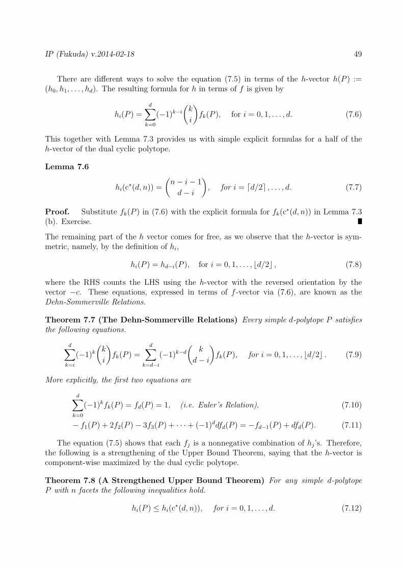
IP (Fukuda) v.2014-02-18 49

There are different ways to solve the equation (7.5) in terms of the h-vector h(P ) :=(h0, h1, . . . , hd). The resulting formula for h in terms of f is given by

hi(P ) =

d∑

k=0

(−1)k−i

(k

i

)fk(P ), for i = 0, 1, . . . , d. (7.6)

This together with Lemma 7.3 provides us with simple explicit formulas for a half of theh-vector of the dual cyclic polytope.

Lemma 7.6

hi(c∗(d, n)) =

(n− i− 1

d− i

), for i = ⌈d/2⌉ , . . . , d. (7.7)

Proof. Substitute fk(P ) in (7.6) with the explicit formula for fk(c∗(d, n)) in Lemma 7.3

(b). Exercise.

The remaining part of the h vector comes for free, as we observe that the h-vector is sym-metric, namely, by the definition of hi,

hi(P ) = hd−i(P ), for i = 0, 1, . . . , ⌊d/2⌋ , (7.8)

where the RHS counts the LHS using the h-vector with the reversed orientation by thevector −c. These equations, expressed in terms of f -vector via (7.6), are known as theDehn-Sommerville Relations.

Theorem 7.7 (The Dehn-Sommerville Relations) Every simple d-polytope P satisfiesthe following equations.

d∑

k=i

(−1)k(k

i

)fk(P ) =

d∑

k=d−i

(−1)k−d

(k

d− i

)fk(P ), for i = 0, 1, . . . , ⌊d/2⌋ . (7.9)

More explicitly, the first two equations are

d∑

k=0

(−1)kfk(P ) = fd(P ) = 1, (i.e. Euler’s Relation), (7.10)

− f1(P ) + 2f2(P )− 3f3(P ) + · · ·+ (−1)ddfd(P ) = −fd−1(P ) + dfd(P ). (7.11)

The equation (7.5) shows that each fj is a nonnegative combination of hj’s. Therefore,the following is a strengthening of the Upper Bound Theorem, saying that the h-vector iscomponent-wise maximized by the dual cyclic polytope.

Theorem 7.8 (A Strengthened Upper Bound Theorem) For any simple d-polytopeP with n facets the following inequalities hold.

hi(P ) ≤ hi(c∗(d, n)), for i = 0, 1, . . . , d. (7.12)

IP (Fukuda) v.2014-02-18 50

Proof. Let P be a simple d-polytope with n facets. The claimed inequalities are trivialfor i = 0 and i = d. By the symmetry of the h-vector, we only need to show

hi(P ) ≤ hi(c∗(d, n)) ≡

(n− i− 1

d− i

), for i = ⌈d/2⌉ , . . . , d.

We use induction on i but with decreasing values. Suppose the theorem is valid for i = k+1(k < d), and consider the case i = k.

We claim two inequalities for h-vectors. First we observe that for any facet F of P andfor any i,

hi(F ) ≤ hi+1(P ). (7.13)

This is valid because we can select a generic c such that all the vertices in F take the objectvalue higher than any other vertices of P . Note that the values hi(F ) and hi+1(P ) areinvariant over choices of c. Secondly, we have

∑

F

hi(F ) = (i+ 1)hi+1(P ) + (d− i)hi(P ). (7.14)

The summation in LHS is over all faces F of P . This equation can be verified once weobserve that every vertex of a face with indegree i in the face has indegree i or i+1 in P . Ifit has indegree i in P , there are exactly (d − i) facets containing it that preserve the sameindegree. If it has indegree i + 1 in P , there are exactly (i + 1) facets containing it thatdecrease its indegree by one.

Now we look at the inductive step for i = k. By the two inequalities (7.14) and (7.13),we have

(k + 1)hk+1(P ) + (d− k)hk(P ) =∑

F

hk(F ) ≤ nhk+1(P ). (7.15)

This implies

(d− k)hk(P ) ≤ (n− k − 1)hk+1(P ), or equivalently, (7.16)

hk(P ) ≤n− k − 1

d− khk+1(P ). (7.17)

Now we use the inductive hypothesis for i = k + 1 to get

hk(P ) ≤n− k − 1

d− khk+1(P ) ≤

n− k − 1

d− k

(n− k − 2

d− k − 1

)=

(n− k − 1

d− k

). (7.18)


While the h-vector of the cyclic polytope is extremely simple, its f -vector is rathercomplicated. The formula can be written explicitly using (7.5), (7.6) and (7.8). We herepresent a formula for f0(c

∗(d, n)) which is quite simple.

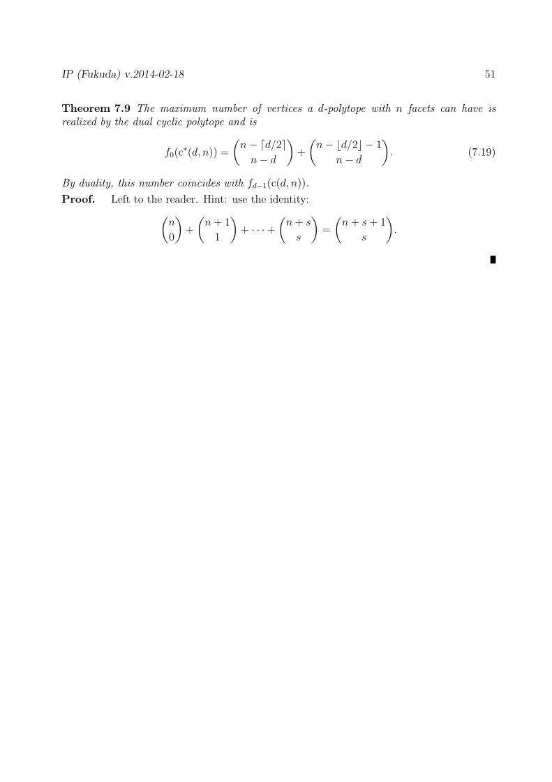
IP (Fukuda) v.2014-02-18 51

Theorem 7.9 The maximum number of vertices a d-polytope with n facets can have isrealized by the dual cyclic polytope and is

f0(c∗(d, n)) =

(n− ⌈d/2⌉

n− d

)+

(n− ⌊d/2⌋ − 1

n− d

). (7.19)

By duality, this number coincides with fd−1(c(d, n)).

Proof. Left to the reader. Hint: use the identity:

(n

0

)+

(n+ 1

1

)+ · · ·+

(n+ s

s

)=

(n + s+ 1

s

).

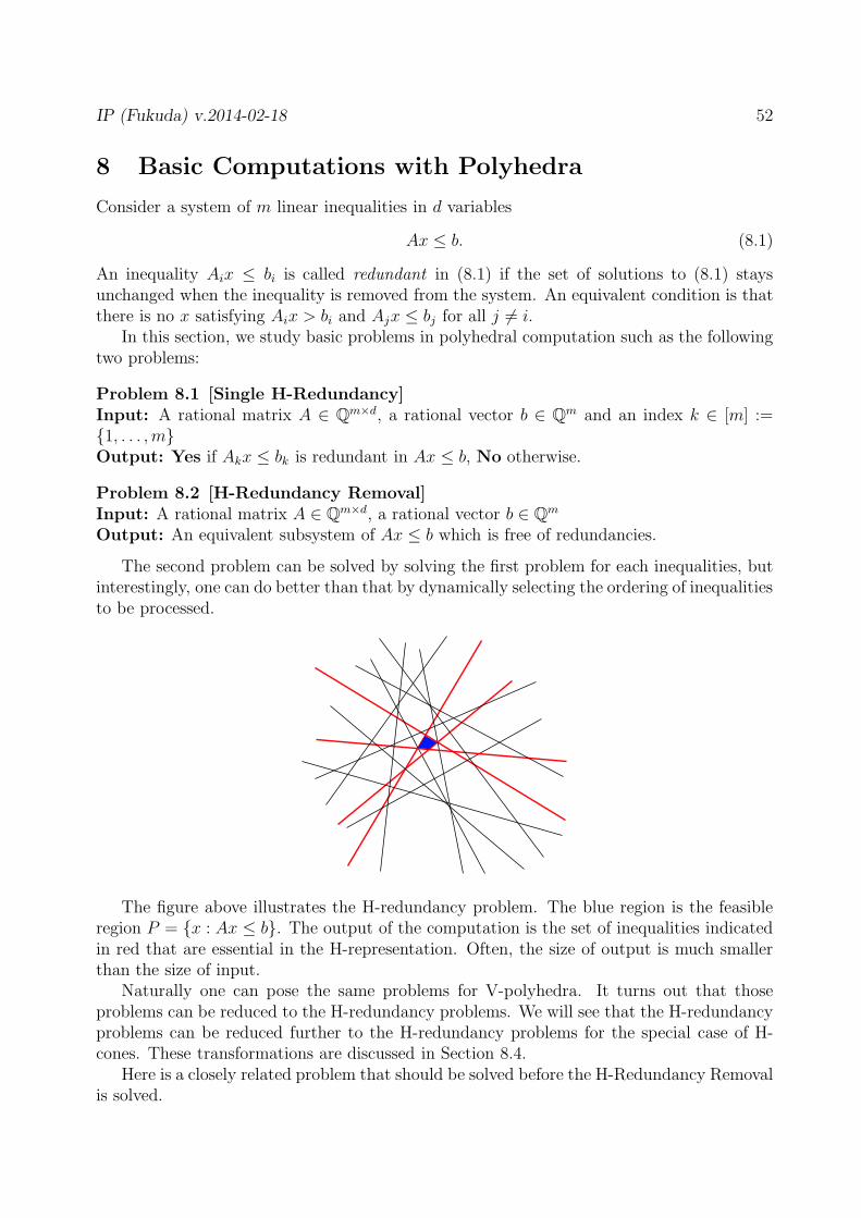
IP (Fukuda) v.2014-02-18 52

8 Basic Computations with Polyhedra

Consider a system of m linear inequalities in d variables

Ax ≤ b. (8.1)

An inequality Aix ≤ bi is called redundant in (8.1) if the set of solutions to (8.1) staysunchanged when the inequality is removed from the system. An equivalent condition is thatthere is no x satisfying Aix > bi and Ajx ≤ bj for all j 6= i.

In this section, we study basic problems in polyhedral computation such as the followingtwo problems:

Problem 8.1 [Single H-Redundancy]Input: A rational matrix A ∈ Qm×d, a rational vector b ∈ Qm and an index k ∈ [m] :=1, . . . , mOutput: Yes if Akx ≤ bk is redundant in Ax ≤ b, No otherwise.

Problem 8.2 [H-Redundancy Removal]Input: A rational matrix A ∈ Qm×d, a rational vector b ∈ Qm

Output: An equivalent subsystem of Ax ≤ b which is free of redundancies.

The second problem can be solved by solving the first problem for each inequalities, butinterestingly, one can do better than that by dynamically selecting the ordering of inequalitiesto be processed.

The figure above illustrates the H-redundancy problem. The blue region is the feasibleregion P = x : Ax ≤ b. The output of the computation is the set of inequalities indicatedin red that are essential in the H-representation. Often, the size of output is much smallerthan the size of input.

Naturally one can pose the same problems for V-polyhedra. It turns out that thoseproblems can be reduced to the H-redundancy problems. We will see that the H-redundancyproblems can be reduced further to the H-redundancy problems for the special case of H-cones. These transformations are discussed in Section 8.4.

Here is a closely related problem that should be solved before the H-Redundancy Removalis solved.

IP (Fukuda) v.2014-02-18 53

Problem 8.3 [H-Dimension]Input: A rational matrix A ∈ Qm×d, a rational vector b ∈ Qm

Output: The dimension of the polyhedron P = x : Ax ≤ b.

A typical algorithm for this computes not only the dimension of P , but also a relative interiorpoint of P , see Section 8.3. One can then embed the polytope in a lower-dimensional spaceso that P becomes full-dimensional.

These problems are much easier than other problems in polyhedral computation such asthe representation conversion between V- and H-representations and computing the volumeof a polytope. In fact, the problems discussed in this section are all polynomially solvablein the size of input.

The main goal of this section is to present many algorithms which are not only polynomial-time but also best possible in terms of the number of LP’s that must be solved, or of thesize of LP’s that must be solved when the number of LP’s to be solved is fixed.

For this purpose, we use the notion of LP complexity, where we count the number ofLP’s and their sizes as a complexity measure. This makes sense only when solving LP’sdominates other computations such as solving systems of linear equations of sizes of sameorder. This applies very well to all problems in this Section.

We denote by LP(d,m) the time necessary to solve any LP with d variables and minequality constraints: max cTx subject to Ax ≤ b, where A is m × d rational matrix.We consider LP(d,m) is an upper bound time measured by big-oh O notation, such asO(md3) or O(e

√d logm). Unlike the usual way to measure the LP complexity using the binary

encoding length L of input, we simply ignore L. The main reason is that practically all ofimplementations of LP algorithms depend hardly on L, but essentially and polynomially ond and m. Further more, we are mostly interested in the case when m is much larger than dand at least as large as 2d. This practical observation leads to that

Assumption 8.4 We assume that LP(d,m) satisfy the following assumptions.

(a) LP(d,m) = LP(d+ c1, m+ c2) for any constants c1 and c2.

(b) LP(d,m) is at least of order md2, that is, Ω(md2).

The first assumption is based on the fact that LP is solvable in a polynomial time. Thesecond assumption is based on the fact that solving a system of linear inequalities is at leastas hard as solving a system of linear equations of the same size (up to constant factor),and the Gaussian elimination has Ω(md2) complexity. This second assumption will be usedthroughout this chapter to argue that the time to solve a linear equality system or to computea rank of an m× d matrix is dominated by LP(d,m).

8.1 Single H-Redundancy Checking

Here we show that Problem 8.1 is linearly equivalent to the linear programming. The onedirection is rather obvious, that is, the Single H-redundancy checking can be done by a singleLP of the same size.

IP (Fukuda) v.2014-02-18 54

Proposition 8.5 Problem 8.1 has No answer if and only if the following LP with I = [m]:

Test(I, k): maximize Akxsubject to

Aix ≤ bi, ∀i ∈ I \ kAkx ≤ bk + 1

(8.2)

has an optimal solution whose optimal value is strictly greater than bk.

Note that the reduction is not only polynomial but linear. Surprisingly, there is a linearreduction from the linear programming (the linear feasibility) to the Single H-redundancy.

Proposition 8.6 The system Ax ≤ b is consistent if and only if a special case of Problem8.1:

is the inequality x0 ≤ 0 redundant in Ax ≤ b x0 and x0 ≤ 0 (8.3)

has No answer.

Proof. Suppose the x0 ≤ 0 is redundant. This is equivalent to the statement thatthere exists no (x, x0) such that Ax ≤ b x0 and x0 > 0. This in turn is equivalent to theinconsistency of Ax ≤ b.

We have shown the linear equivalence of the Single H-redundancy checking and theLP. This implies that any redundancy checking algorithm is at least as powerful as an LPalgorithm.

In the next section, we will see that removing all H-redundancies can be easier thansolving m LP’s of size (d,m) that takes time m×LP(d,m) if the system is highly redundant.

8.2 H-Redundancy Romoval

Here we discuss the problem of removing all redundancies from an H-representation of apolyhedron, i.e., Problem 8.2.

We shall assume that the input of Problem 8.2 is “clean” in the sense that the underlyingpolyhedron P = x : Ax ≤ b is full-dimensional and no inequality is a positive multiple ofanother one. This assumption can be met if the preprocessing is done, namely, by embeddingthe polyhedron in an appropriate subspace. This part will be discussed in Section 8.3.

As we have seen in Section 8.1, removing all redundancies can be done in m× LP(d,m)time. Can one do better than this? Here we present an algorithm due to Clarkson [15] whichruns much faster than the naive algorithm when the number s of nonredundant inequalitiesis small relative to m.

Let Ax ≤ b be an input system. We assume that a point z ∈ Qd is given satisfyingAz < b, an interior point of the feasible region P = x : Ax ≤ b. At the general stage ofthe algorithm, we have already detected a row index set I such that the inequality Aix ≤ biis nonredundant for Ax ≤ b, for each i ∈ I. Let j be an row index which is not tested yet,i.e. j ∈ [m] \ I. Clarkson’s algorithm either detects kth inequality is redundant or finds arow index j ∈ [m] \ I such that Ajx ≤ bj is nonredundant.

IP (Fukuda) v.2014-02-18 55

procedure Clarkson(A,b,z,I,k)begin

test whether Akx ≤ bk is redundant in AI∪kx ≤ bI∪kby solving the LP Test(I ∪ k, k) with optimal solution x∗

if nonredundant then(c1) return (1, RayShoot(A,b,z,x∗ − z)) //Returns an essential index

else(c2) return (0, k) //Returns an redundant index

endifend

Here, the procedure RayShoot(A,b,z,r) returns an index j of a facet-inducing hyperplanex : Ajx = bj hit by the ray starting from z along the direction r. It can be easilyimplemented by analyzing symbolically the ray starting from z + (ǫ, ǫ2, . . . , ǫd)T along thedirection r for sufficiently small ǫ > 0.

x*

k

z

x*

k

j

AI x ≤ b

I AI x ≤ b

I

Figure 8.1: Clarkson’s Algorithm: Left (k is redundant), Right(An essential j is found)

Exercise 8.1 Write a procedure RayShoot(A,b,z,r) following the specification above. Itshould be specific enough to be implemented with high level computer languages like C andC++.

Here is the complete algorithm to remove all redundancies. We assume that an interiorpoint z of P = x : Ax ≤ b is given.

procedure RedundacyRemovalClarkson(A,b,z)begin

set I := ∅, J := [m]repeat

select an index k from J

IP (Fukuda) v.2014-02-18 56

(α, j) =Clarkson(A,b,z,I,k)if α = 1 then I := I ∪ j //Increment the essential set IJ := J \ j

until J = ∅return I

end

Theorem 8.7 The complexity of Clarkson’s algorithm to find a minimal equivalent subsys-tem of Ax ≤ b is m×LP(d, s) where s is the number of nonredundant constraints in Ax ≤ b.

Proof. At each step, Clarkson’s algorithm either finds an row index k to be a redundantinequality row index or discovers a new row index j 6= k for which Ajx ≤ bj is essential.Since the size of an LP solved has d variables and at most s+ 1 constraints, the complexityfollows. Note that the complexity of a ray shooting is O(md). Since the number of rayshooting is at most s, the total time O(smd) of ray shooting is dominated by m× LP(d, s).

8.3 Computing H-Dimension

It is often important to know the dimension of a polyhedron. When a polyhedron is a V-polyhedron with representation, it is very easy to compute its dimension. More precisely, ifP is a V-polyhedron for some generator matrices d× s matrix V and d× t matrix R, i.e.,

P = x : x = V λ+Rµ, 1Tλ = 1, λ ≥ 0, µ ≥ 0,

then the dimension of P is easily computable, namely by the formula,

dimP = rank

[V R1T 0T

]− 1.

However, for an H-polyhedronP = x : Ax ≤ b

its dimension is nontrivial to compute. Why nontrivial? It is simply because if one knows thedimension, one can decide whether P is empty or not, that is the linear feasibility problem,equivalent to LP. Then, the next question is how many LP’s one has to solve to determinethe dimension. Obviously, at least one. It is not hard to see that at most m LP’s is sufficient.

In this section, we show that one can compute the dimension by solving at most d LP’s.As a byproduct, one also finds a point in the relative interior of P .

The first step is to try to find an interior point of P . If it is successful, the dimension isof course d. One can easily see that the following LP will detect the full-dimensionality:

maximize x0

subject toAx+ 1x0 ≤ b,

x0 ≤ 1.

(8.4)

More precisely, we have three cases, depending on the outcome of the LP. Let x∗ be anoptimal solution and let x∗

0 be the optimal value.

IP (Fukuda) v.2014-02-18 57

Case 1: x∗0 > 0 . In this case, an optimal solution x∗ is an interior point and dimP = d.

Case 2: x∗0 < 0 . In this case, the polyhedron P is empty and dimP = −1.

Case 3: x∗0 = 0 . In this case, the polyhedron P is neither full-dimensional nor empty.

In case 3, we must do more computation. For that, we can make use of a dual optimalsolution (s∗, t∗) for the dual LP:

minimize bT s + tsubject to

AT s = 0,1T s + t = 1,

s ≥ 0, t ≥ 0.

(8.5)

By strong duality, the dual optimal value is zero. This means that s∗ cannot be totally zero.Let I = i : s∗i > 0. By the complementary slackness, at any feasible solution (x, x0) withx0 = 0 (i.e., at any solution x for Ax ≤ b), every inequality in AIx ≤ bI must be tight.We might do even further. By Gaussian elimination, we can recognize all other inequalitiesin Ax ≤ b that are forced to be equalities provided AIx = bI . Let us merge I with thesedependent equality indices, and call it I. Now we are ready to solve another LP to find moreimplicit equalities in the remaining system. For this, let C := I, and D := [m] \ C, and setup an LP:

maximize x0

subject toACx = bC ,ADx +1x0 ≤ bD,

x0 ≤ 1.

(8.6)

At an optimal solution (x∗, x∗0), there are only two cases because x∗ cannot be negative this

time. When x∗0 > 0, the solution x∗ is a relative interior point, and the dimension of P is

easily computed. It is d minus the maximum number of independent equalities in AIx = bI .When x∗

0 = 0, we do essentially the same thing as we did at the very first stage: use thedual optimal solution to recognize implicit equalities in ADx ≤ bD. Then extend themwith possible dependent equalities. Another LP should be solved with extended C and itscomplement D. Since every time an LP is solved, at least one independent implicit equalityis found. This shows that at most d LP’s will be solved until a relative interior point isfound. Thus we have:

Theorem 8.8 Problem 8.3 can be solved in d× LP(d,m) time.

Exercise 8.2 (Embedding a Polyhedron) Given a point z in the relative interior of P =Ax ≤ b, explain a method to embed P to a lower dimensional space so that it is full-dimensional there.

IP (Fukuda) v.2014-02-18 58

8.4 Reducing the Nonhomogeneous Case to the HomogeneousCase

We define the homogenization of a system Ax ≤ b as the new system with one extra non-negative variable x0,

Ax ≤ b x0 and x0 ≥ 0. (8.7)

Proposition 8.9 Let Ax ≤ b be a consistent system. An inequality Aix ≤ bi is redundantin the system if and only if the corresponding inequality Aix ≤ bi x0 is redundant in thehomogenization.

Exercise 8.3 Prove the proposition above. Show that the assumption that Ax ≤ b beingconsistent is necessary by providing a small example in which Aix ≤ bi is redundant inAx ≤ b but Aix ≤ bi x0 is nonredundant in the homogenization.

What we have shown above is that the H-redundancy removal for cones solves the moregeneral problem for polyhedra.

What about for a V-polyhedron? Can we reduce the redundancy removal for V-polyhedrato the one for V-cones? Consider a V-polyhedron with generator pair (V,R) where V ∈ Qd×s

and R ∈ Qd×t:

PV (V,R) := x : x = V λ +Rµ, 1Tλ = 1, λ ≥ 0, µ ≥ 0.

Let vj denote the jth column of V , and rk denote the kth column of R. We say a generatorvj (rk) is redundant for PV (V,R) if removing vj from V (rk from R, respectively) does notalter the polyhedron.

Proposition 8.10 For V ∈ Qd×s and R ∈ Qd×t, a generator vj (rk) is redundant for

PV (V,R) if and only if the corresponding generator

[vj1

](

[rj0

], respectively) is redundant in

the homogenization

CV (R) := x : x = Rµ, µ ≥ 0,where R =

[V R1T 0T

].

Proof. The proof is straightforward. Left to the reader.

Now, we know that both the H-redundancy removal and the V-redundancy romovalfor cones are as powerful as those for polyhedra. Finally, we have the duality of H- andV-redundancy removals which implies that an algorithm for one problem solves both.

Proposition 8.11 Let A ∈ Qm×d. Then, each inequality Aix ≤ 0 is redundant in Ax ≤ 0if and only if the corresponding generator AT

i is redundant for CV (AT ).

Proof. Let Aix ≤ 0 be redundant in Ax ≤ 0. This means there exists no x such thatAix > 0 and Ajx ≤ 0 for all j 6= i. By the Farkas Lemma (Exercise 3.4), this is equivalentto the existence of µ ≥ 0 such that AT

i =∑

j 6=i ATj µj. This is equivalent to saying AT

i is

redundant for CV (AT ). This completes the proof.

Exercise 8.4 (Dimensionality and Linearity) Given a point z in the relative interior ofCH(A) := Ax ≤ 0, explain a method to find a basis of the linearity space of CV (A

T ).

IP (Fukuda) v.2014-02-18 59

9 Polyhedral Representation Conversion

The Minkowski-Weyl Theorem, Theorem 3.9, shows that every convex polyhedron has tworepresentations, an H-representation and a V-representation. The associated problem ofcomputing a (minimal) V-representation from a H-representation or its converse is knownas the representation conversion problem for polyhedra.

One important characteristic of the representation conversion problem is that the size ofoutput is not easy to measure in terms of the size of input. For example, for a d-cube having2d facets and 2d vertices, the H-to-V conversion has output whose size is exponential in theinput size and the V-to-H conversion has the output size very small relative to the inputsize.

Given this diversity of output sizes, an ideal algorithm for the conversion problem mustbe sensitive to the output size, as opposed to optimal for the worst-case output size of agiven input size. An algorithm is called output-polynomial if its running time is bounded bya polynomial function of both the input size and the output size.

Also, we must take account of the memory footprint. Some algorithms need to store alarge amount of data in the memory, while others simply do not store anything except theinput data and a few more. We say an algorithm is compact if its space is bounded by apolynomial function of the input size only.

One might call an algorithm ideal if it is both compact and output-polynomial. Forthe representation conversion problem, there is no known output-polynomial algorithm ingeneral. However for the special cases of various nondegeneracy, compact output-polynomialalgorithms are known, typically based on the reverse-search paradigm, see Section 9.2.

9.1 Incremental Algorithms

In this section, we present a classical finite algorithm, known as the double description (DD)method [40]. It can be also considered as a constructive proof of Minkowski’s Theorem, theimplication of (a) =⇒ (b) in the Minkowski-Weyl Theorem, Theorem 3.10. The algorithmis not output-polynomial as it was shown by Bremner [10]. However, it is extremely usefulfor certain representation conversion problems, in particular, for highly degenerate inputs.

Suppose that an m × d matrix A is given, and let C(A) = x : Ax ≤ 0. We call anyvector r ∈ C(A) a ray of C(A). The DD method is an incremental algorithm to construct ad× n matrix R such that (A,R) is a DD pair.

Let K be a subset of the row indices 1, 2, . . . , m of A and let AK denote the submatrixof A consisting of rows indexed by K. Suppose we already found a generating matrix R forC(AK), or equivalently (AK , R) is a DD pair. If A = AK , clearly we are done. Otherwisewe select any row index i not in K and try to construct a DD pair (AK+i, R

′) using theinformation of the DD pair (AK , R). Note that K + i is a simplified notation for K ∪ i.

Once this basic procedure is described, we have an algorithm to construct a generatingmatrix R for C(A). This procedure can be easily understood geometrically and the readeris strongly encouraged to draw some simple example in the three dimensional space.

IP (Fukuda) v.2014-02-18 60

The newly introduced inequality Ai x ≤ 0 partitions the space Rd into three parts:

H+i = x ∈ Rd : Ai x > 0

H0i = x ∈ Rd : Ai x = 0

H−i = x ∈ Rd : Ai x < 0.

(9.1)

Let J be the set of column indices of R and let rj denote the jth column of R. The rays rj(j ∈ J) are then partitioned into three parts:

J+ = j ∈ J : rj ∈ H+i

J0 = j ∈ J : rj ∈ H0i

J− = j ∈ J : rj ∈ H−i .

(9.2)

We call the rays indexed by J+, J0, J− the positive, zero, negative rays with respect to i,respectively. To construct a matrix R′ from R, we generate new |J+| × |J−| rays lying onthe ith hyperplane H0

i by taking an appropriate positive combination of each positive ray rjand each negative ray rj′ and by discarding all positive rays.

The following lemma ensures that we have a DD pair (AK+i, R′), and provides the key

procedure for the most primitive version of the DD method.

Lemma 9.1 (Main Lemma for Double Description Method) Let (AK , R) be a DDpair and let i be a row index of A not in K. Then the pair (AK+i, R

′) is a DD pair,where R′ is the d× |J ′| matrix with column vectors rj ( j ∈ J ′ ) defined by

J ′ = J− ∪ J0 ∪ (J+ × J−), and

rjj′ = (Ai rj)rj′ − (Ai rj′)rj for each (j, j′) ∈ J+ × J−.

Proof. Let C = C(AK+i) and let C ′ be the cone generated by the matrix R′. We mustprove that C = C ′. By the construction, we have rjj′ ∈ C for all (j, j′) ∈ J+ × J− andC ′ ⊂ C is clear.

Let x ∈ C. We shall show that x ∈ C ′ and hence C ⊆ C ′. Since x ∈ C, x is a nonnegativecombination of rj ’s over j ∈ J , i.e., there exist λj ≥ 0 for j ∈ J such that

x =∑

j∈Jλjrj . (9.3)

If there is no positive λj with j ∈ J+ in the expression above then x ∈ C ′. Suppose there issome k ∈ J+ with λk > 0. Since x ∈ C, we have Ai x ≤ 0. This together with (9.3) impliesthat there is at least one h ∈ J− with λh > 0. Now by construction, hk ∈ J ′ and

rhk = (Ai rh)rk − (Ai rk)rh. (9.4)

By subtracting an appropriate positive multiple of (9.4) from (9.3), we obtain an expressionof x as a positive combination of some vectors rj (j ∈ J ′) with new coefficients λj where thenumber of positive λj ’s with j ∈ J+ ∪ J− is strictly smaller than in the first expression. Aslong as there is j ∈ J+ with positive λj, we can apply the same transformation. Thus wemust find in a finite number of steps an expression of x without using rj with j ∈ J+. Thisproves x ∈ C ′, and hence C ⊆ C ′.

IP (Fukuda) v.2014-02-18 61

This algorithm can be used to prove Minkowski’s Theorem constructively.

Proof. (of Theorem 3.10) By Lemma 9.1, it is sufficient to show that one can find aninitial DD pair (AK , R) for some K. The trivial case is when K = ∅ and C(AK) = Rd. Inthis case, the set of 2d vectors R = e1,−e1, e2,−e2, . . . , ed,−ed generates the space Rd bytheir nonnegative combinations. (Actually, one can find d+ 1 vectors which positively spanRd. How?) This completes the proof.Here we write the DD method in procedural form.

procedure DoubleDescriptionMethod(A);begin

Obtain any initial DD pair (AK , R)while K 6= 1, 2, . . . , m dobegin

Select any index i from 1, 2, . . . , m \KConstruct a DD pair (AK+i, R

′) from (AK , R)/* by using Lemma 9.1 */

R := R′ K := K + i;endOutput R

end.

The DD method given here is very primitive, and the straightforward implementation isnot quite useful, because the size of J increases very fast and goes beyond any tractablelimit. One reason for this is that many (perhaps, most) vectors rjj′ the algorithm generates(defined in Lemma 9.1), are unnecessary. To avoid generating redundant generators, westore and update the adjacency of generators. Such a refinement can reduce the size of theoutput drastically.

(AK

, R) (AK+i

, R')

New rays should be generated

only for adjacent pairs ( , )

J -

J+

hi

Figure 9.1: The Double Description Algorithm

IP (Fukuda) v.2014-02-18 62

Figure 9.1 depicts a general step of adding the ith inequality with a refined doubledescription algorithm. The polytopes should be considered as a cut section of 4-dimensionalpointed cones with some hyperplane so that each vertex represents one dimensional extremeray starting from the origin.

Two generators are said to adjacent if the common set of active constraints is maximalamong all pairs of generators. This means that the line segment connecting a adjacent pairmeets the new hyperplane hi = x : Aix = 0 at a point lying on a minimal face of the coneC(AK+i). It is easy to see that such a point must be in any V-representation.

The double description algorithm at the ideal form not generating any redundant gener-ators is still not easy to analyze. The main problem is that the size of a V-representationof intermediate cone is not easy to estimate. The size also depends heavily on the insertionorder of constraints.

Here are somewhat surprising behaviors of the refined double desciption method withrespect to different insertion orders. In the figure below, the input is (the homogenized coneof) a 15-dimensional polytope with 32 facets. The output is a list of 368 vertices. It isimportant to note that the conversion is highly degenerate, meaning that the number ofactive inequalities at each output vertex is much higher than the dimension.

We consider the five different orderings of the inequalities. The ordering lexmin is simplysort the rows of A by lexicographic ordering, comparing the first component first, then thesecond in case of tie, and the third, etc. The ordering maxcutoff (mincutoff)is a dynamicordering in which at each iteration the next inequality is selected to maximize (minimize)the size |J+|. The lexmin is a sort of shelling ordering which appears to perfom the bestamong all orderings tested.

20 22 24 26 28 30 32Iteration

250

500

750

1000

1250

1500

Size INTERMEDIATE SIZES FOR CCP6

maxcutoff

mincutoffrandom

lexmin

Figure 9.2: Comparison of Intermediate Sizes for a Degenerate Input

IP (Fukuda) v.2014-02-18 63

A more striking comparison is given below where the input is a 10-dimensional crosspolytope with 210 facets. The output is a list of 20 vertices. The highest peak is attainedby maxcutoff ordering, following by random and mincutoff. The ordering lexmin is the bestamong all and the peak intermediate size is less than 30. Note that the graph of lexmin istoo low to see it in the figure below.

200 400 600 800 1000

5000

10000

15000

20000

25000

30000

Iteration

Size

Random

Maxcutoff

Mincutoff

Figure 9.3: Comparison of Intermediate Sizes for a Highly Degenrate Input

9.2 Pivoting Algorithms

One can design pivoting algorithms to visit all vertices of a convex polytope systematically.The idea is quite simple. The graph of a convex polytope is connected, and in fact d-connected if the polytope is d-dimensional, due to Balinski [7]. Thus, one can trace thegraph systematically until no new vertex can be found.

A polytope P and its graph (1-skeleton)

IP (Fukuda) v.2014-02-18 64

Historically, there are many pivoting algorithms proposed by Balinski [6], Murty [42], Dyerand Proll [19], etc. The weakness of pivoting algorithms is that when the polytope is degen-erate, i.e., non-simple, pivoting may not be able to trace the graph of a polytope efficiently.Typical way to resolve degeneracy is a symbolic perturbation of constraints which may createan exponentially large number of new extreme points. Under the nondegeneracy assumptionthat the number of active constraints at each vertex is exactly d, the algorithm due to Dyerand Proll [19] is an output-polynomial algorithm. Yet, it must store all visited vertices inmemory and thus is not a compact algorithm.

In this section, we present a compact output-polynomial algorithm for the nondegeneratecase, based on the reverse search technique due to Avis and Fukuda.

The main idea is to reverse the simplex method from the optimal vertex in all possibleways. Here the objective function is set to any generic one so that the optimal vertex isunique and no edge of the polytope is parallel to an objective contour.

!!

!$

"*

#"

$"

min x1 + x2 + x3

Also, another important thing is to make sure that the simplex algorithm is finite and selectsa next pivot uniquely at each vertex. This can be achieved, for example, by employing theminimum index rule (Bland’s rule). Under these, the edges used by the refined simplexmethod form a directed spanning tree of the graph G(P ) of a polytope P rooted at theoptimal vertex. We will see that the resulting algorithm enumerates all f0 vertices in timeO(mdf0) and O(md)-space under nondegeneracy when the input H-polytope is given by minequalities in d variables. Thus, it is compact and output-polynomial.

For a formal description, let us define two functions. A finite local search f for a graphG = (V,E) with a special node s ∈ V is a function: V \ s → V satisfying

(L1) v, f(v) ∈ E for each v ∈ V \ s, and

IP (Fukuda) v.2014-02-18 65

(L2) for each v ∈ V \ s, ∃k > 0 such that fk(v) = s.

For example, let P = x ∈ Rd : A x ≤ b be a simple polytope, and cTx be any genericlinear objective function. Let V be the set of all vertices of P , s the unique optimal, and f(v)be the vertex adjacent to v selected by the simplex method which selects a pivot uniquely ifv is not the optimal vertex.

A adjacency oracle or simply A-oracle Adj for a graph G = (V,E) is a function (where δa upper bound for the maximum degree of G) satisfying:

(i) for each vertex v and each number k with 1 ≤ k ≤ δ the oracle returns Adj(v, k), avertex adjacent to v or extraneous null (null),

(ii) if Adj(v, k) = Adj(v, k′) 6= 0 for some v ∈ V , k and k′, then k = k′,

(iii) for each vertex v, Adj(v, k) : Adj(v, k) 6= 0, 1 ≤ k ≤ δ is exactly the set of verticesadjacent to v.

For example, when P = x ∈ Rd : A x ≤ b is a simple polytope, let V be the set of allvertices of P , δ be the number of nonbasic variables and Adj(v, k) be the vertex adjacent tov obtained by pivoting on the kth nonbasic variable at v.

Now we are ready to describe a general reverse search algorithm to generate all verticesof the underlying graph G assuming that the two functions f and Adj are given.

procedure ReverseSearch(Adj,δ,s,f);v := s; j := 0; (* j: neighbor counter *)repeat

while j < δ doj := j + 1;

(r1) next := Adj(v, j);if next 6= null then

(r2) if f(next) = v then (* reverse traverse *)v := next; j := 0endif

endifendwhile;if v 6= s then (* forward traverse *)

(f1) u := v; v := f(v);(f2) j := 0; repeat j := j + 1 until Adj(v, j) = u (* restore j *)

endifuntil v = s and j = δ

We can evaluate the complexity of reverse search above as follows. Below we denote byt(f) and t(Adj) the time to evaluate the functions f and Adj, respectively.

Theorem 9.2 Suppose that a local search (G, s, f) is given by an A-oracle. Then the timecomplexity of ReverseSearch is O(δ t(Adj)|V |+ t(f)|E|).

IP (Fukuda) v.2014-02-18 66

Proof. It is easy to see that the time complexity is determined by the total time spentto execute the four lines (r1), (r2), (f1) and (f2). The first line (r1) is executed at most δtimes for each vertex, and the total time spent for (r1) is O(δ t(Adj)|V |). The line (r2) isexecuted as many times as the degree deg(v) for each vertex v, and thus the total time for(r2) is O(t(f)|E|). The third line (f1) is executed for each vertex v in V \ s, and hence thetotal time for (f1) is O(t(f)(|V |− |S|)). Similarly, the total time for (f2) is O(δ t(Adj)(|V |)).Since |V | ≤ |E|, by adding up the four time complexities above, we have the claimed result.

Corollary 9.3 Suppose that a local search (G, s, f) is given by an A-oracle. Then the timecomplexity of ReverseSearch is O(δ (t(Adj) + t(f))|V |). In particular, if δ, t(f) and t(Adj)are independent of the number |V | of vertices in G, then the time complexity is linear in theoutput size |V |.

Proof. The claim follows immediately from Theorem 9.2 and the fact that 2|E| ≤ δ|V |.

One can improve the complexity of reverse search algorithms by exploiting special struc-tures. We give the best known complexity of reverse search for the representation conversionfor convex polytopes without proof, see [4] for details.

Theorem 9.4 There is an implementation of reverse search algorithm to enumerate allvertices of a nondegenerate H-polytope P = x : Ax ≤ b in time O(mdf0) and space O(md),where A ∈ Qm×d, b ∈ Qm and f0 is the number of vertices of P . In particular, it is a compactoutput-polynomial algorithm for nondegenerate inputs.

There are many applications of reverse search in geometry and combinatorics, see [5].Finally, what is the difference between reverse search and depth-first search? The quick

answer is: reverse search is a memory-free search while depth-first search must store all nodesvisited so far to distinguish those vertices from the rest. In other words, reserve search isdepth-first search applied to a unique spanning tree of the graph defined by local searchfunction f .

9.3 Pivoting Algorithm vs Incremental Algorithm

• Pivoting algorithms, in particular the reverse search algorithm (lrs, lrslib [2]), workwell for high dimensional cases.

• Incremental algorithms work well for low (say, up to 12) dimensional cases and highlydegenerate cases. For example, the codes cdd/cddlib [22] and porta [13] are imple-mented for highly degenerate cases and the code qhull [8] for low (up to 10) dimensionalcases.

• The reverse search algorithm seems to be the only method that scales very efficientlyin massively parallel environment.

• Various comparisons of representation conversion algorithms and implementations canbe found in the excellent article [3] by Avis, Bremner and Seidel.

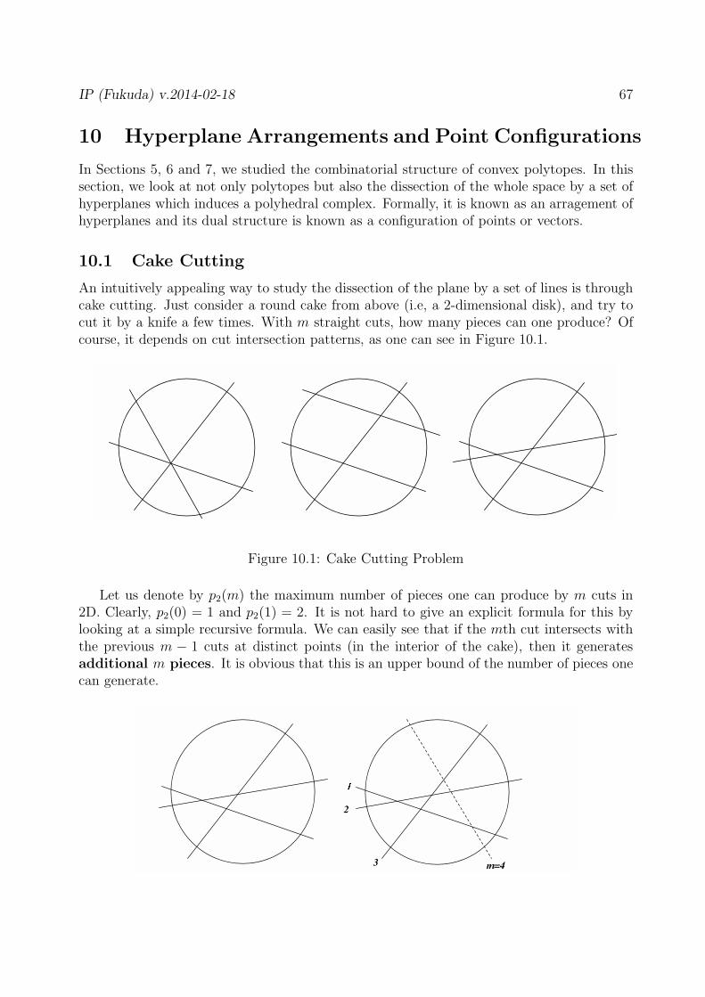
IP (Fukuda) v.2014-02-18 67

10 Hyperplane Arrangements and Point Configurations

In Sections 5, 6 and 7, we studied the combinatorial structure of convex polytopes. In thissection, we look at not only polytopes but also the dissection of the whole space by a set ofhyperplanes which induces a polyhedral complex. Formally, it is known as an arragement ofhyperplanes and its dual structure is known as a configuration of points or vectors.

10.1 Cake Cutting

An intuitively appealing way to study the dissection of the plane by a set of lines is throughcake cutting. Just consider a round cake from above (i.e, a 2-dimensional disk), and try tocut it by a knife a few times. With m straight cuts, how many pieces can one produce? Ofcourse, it depends on cut intersection patterns, as one can see in Figure 10.1.

Figure 10.1: Cake Cutting Problem

Let us denote by p2(m) the maximum number of pieces one can produce by m cuts in2D. Clearly, p2(0) = 1 and p2(1) = 2. It is not hard to give an explicit formula for this bylooking at a simple recursive formula. We can easily see that if the mth cut intersects withthe previous m − 1 cuts at distinct points (in the interior of the cake), then it generatesadditional m pieces. It is obvious that this is an upper bound of the number of pieces onecan generate.

2

3 m=4

IP (Fukuda) v.2014-02-18 68

Is this upper bound attainable? We argue that this is always attainable by placingcuts properly. A 2D cake cutting with m cuts is defined to be nondegenerate if any twodistinct cuts intersect in the interior of the cake and no three distinct cuts have a commonintersection. For any m, nondegenerate cuts exist. Just place m cuts so that no two cutsare parallel and no three cuts intersect. If some two cuts do not intersect in the interior ofthe cake, just dilate the cake (centered at the origin) without changing the cut placements.If the dilation is large enough, all intersections of the lines will be placed inside the cake.Then, shrink the whole space so that the cake becomes the original size.

This observation leads to a simple recursion:

p2(m) = p2(m− 1) +m (10.1)

which implies

p2(m) = p2(0) + 1 + 2 + · · ·+m = 1 +(m+ 1)m

2. (10.2)

Now we go up to one higher dimension. The cake looks like a 3-dimensional ball, and wetry to cut out the largest number of pieces withm cuts. We now imagine how a “watermelon”can be dissected into pieces by a knife into pieces, see Figure 10.2. (A cut does not go throughthe center although the figure shows such a case.)

Figure 10.2: 3-Dimensional Cake Cutting Problem

Let us denote by p3(m) the maximum number of pieces one can produce by m cutsin 3 dimension. Can one write a simple recursive formula for p3(m)? Yes, it is possible,once one notices that the cut section at mth cut in the 3D cake could look like a 2D cakecutting at (m− 1)st step, as long as the mth cut intersects with the previous (m− 1) cutsat distinct lines. A key observation is that the number of 2D pieces at the cut section isexactly the increment of the number of pieces by mth cut. Thus, when the mth cut section

IP (Fukuda) v.2014-02-18 69

is nondegenerate, the increment is largest and thus the observation leads to the recursion

p3(m) = p3(m− 1) + p2(m− 1) (10.3)

= p3(m− 1) + 1 +m(m− 1)

2

= p3(0) +m+

m∑

i=1

i(i− 1)

2

= 1 +m+1

2

(m∑

i=1

i2 −m∑

i=1

i

)

= 1 +m+1

6(m+ 1)

(m+

1

2

)m−

1

4m(m+ 1). (10.4)

(Recall the identity:

m∑

i=1

i2 =1

6(m+ 1)(2m+ 1)m )

We have two explicit formulas, one for 2D (10.2) and the other for 3D (10.4). Can we guessa general formula for pd(m)? Well, not quite easy to guess from what we have. But, it ismuch easier once we rewrite the two equations in the following form:

p2(m) =

(m

0

)+

(m

1

)+

(m

2

)

p3(m) =

(m

0

)+

(m

1

)+

(m

2

)+

(m

3

).

(10.5)

Exercise 10.1 Verify the correctness of the equations (10.5).

Now, we are ready to prove the general cake cutting theorem.

Theorem 10.1 The number pd(m) of the maximum number of pieces dissected from thed-dimensional ball by m (hyperplane) cuts is given by

pd(m) =

d∑

i=0

(m

i

). (10.6)

Proof. We prove the correctness of the formula and the fact that the the value is attainedby any nondegenerate cake cut, by induction on d. Here, we say a d-dimensional cake cuttingof a d-ball (cake) with m cuts is defined to be nondegenerate if any d distinct cuts intersectin the interior of the cake and no (d + 1) distinct cuts have a common intersection. Theformula is correct for d = 2 and attained by any nondegenerate cutting. Consider anyunknown case d assuming that the formula is correct for any smaller dimension. First of all,m = 0, the formula pd(m) is correct that is 1. Here we use second induction on m. Considerany unknown case m assuming that the formula is correct for any smaller values of m. Byextending the recursion (10.3), we have

pd(m) = pd(m− 1) + pd−1(m− 1). (10.7)

IP (Fukuda) v.2014-02-18 70

By induction hypothesis, one can apply the formula to the RHS and we have:

pd(m) =

(m− 1

0

)+

(m− 1

1

)+ · · ·+

(m− 1

d

)

+

(m− 1

0

)+ · · ·+

(m− 1

d− 1

).

Finally, since(m−1−1

)= 0, the last equation above leads to

pd(m) =d∑

k=0

((m− 1

k

)+

(m− 1

k − 1

))

=

d∑

k=0

(m

k

). (10.8)


10.2 Arrangements of Hyperplanes and Zonotopes

Cake cutting is a less formal way of presenting the mathematical notion of arrangements ofhyperplanes in Rd. A finite family A = hi : i = 1, 2, . . . , m of hyperplanes in Rd is calledan arrangement of hyperplanes.

h1

h2

h3

h4

h5

We are mostly interested in combinatorial structures underlying hyperplane arrange-ments. For this, it is convenient to define the partition of the space Rd into three sets:

h+i = x : Ai x < bi, (10.9)

h0i = x : Ai x = bi, (10.10)

h−i = x : Ai x > bi. (10.11)

IP (Fukuda) v.2014-02-18 71

h1

h2

h3

h4

h5

+−

−

−++

_

+

_

+

(0-0-+) (+++++)

(++++0)

There is a natural way to associate each point x in the space Rd with the sign vectorσ(x) ∈ −, 0,+m defined by:

σ(x)i =

+ if x ∈ h+i

0 if x ∈ h0i

− if x ∈ h−i

i ∈ E.

The set of points with a given sign vector is a relatively open polyhedron, is called a openface of the arrangement, and its topological closure is called a face of the arrangement. Thefull dimensional faces are called the cells or regions of the arrangement. The set of all facesforms a polyhedral complex, called the complex of the arrangement . One can represent thefacial incidence in the complex by a binary relation among sign vectors. For two sign vectorsX, Y ∈ −, 0,+m, we say X conforms to Y (denoted as X 4 Y ) if i ∈ [m] and Xi 6= 0implies Xi = Yi. The poset σ(Rd) := σ(x) : x ∈ Rd ordered by conformal relation isa combinatorial representation of the complex. This poset is the face poset F(A) of thearrangement A.

The poset F(A) behaves nicely if all the hyperplanes contains the origin. An arrangementof hyperplanes in which all its hyperplanes contain the origin 0 is called a central arrangementof hyperplanes .

h1

h2

h3

0

h4

+-

- + + -

-+

For example, F(A) contains the zero vector 0 which is the unique smallest element. Also,it is symmetric with respect to the origin: if a sign vector X is in F(A), its negative −X isin F(A). By adding the artificial greatest element 1 of all 1’s to F(A), we obtain what wecall the face lattice F(A) of the central arrangement. We will see this lattice is isomorphicto the lattice of a very special polytope.

IP (Fukuda) v.2014-02-18 72

Let A be a central arrangement of hyperplanes represented by a matrix A, i.e, hi =x : Ai x = 0, ∀i = 1, . . . , m. Geometrically, it is convenient to look at the cut sectionof the arrangement with the unit (d − 1)-sphere Sd−1 := x ∈ Rd : ||x|| = 1, where eachhyperplane becomes a (d−2)-sphere si := hi∩Sd−1. Thus, the cut section is an arrangementof (d − 2)-spheres in the unit sphere Sd−1. The complex of the arrangement is essentiallyrepresented in the sphere arrangement, namely, σ(Rd) = σ(Sd) ∪ 0.

S1

S2

S4

S3

+-

+ -

+-

+-

(-+++)

(00++)

(-0++)

Consider the following H-polyhedron given by 2m inequalities:

PA = x : yT A x ≤ 1, ∀ y ∈ −1,+1m.

Theorem 10.2 Let A be a column full rank matrix representing a central arrangement A.Then PA is a polytope, and the face lattice F(A) of A is isomorphic to the face lattice of thepolytope PA.

The central arrangement A and the polytope PA

The polar of the polytope PA is a very special polytope. In fact, it is a zonotope.

(PA)∗ = convyTA ∈ Rd : y ∈ −1,+1m

= yTA ∈ Rd : y ∈ [−1,+1]m

= L1 + L2 + · · ·+ Lm,

where each generator Li is the line segment [−Ai, Ai].

IP (Fukuda) v.2014-02-18 73

(PA)*

10.3 Face Counting Formulas for Arrangements and Zonotopes

We denote by fk(A) the number of k-dimensional faces of an arrangement A of hyperplanesin Rd. We assume all arrangements are central and thus can be seen as a sphere arrangementin Sd−1.

S1

S2

S4

S3

+-

+ -

+-

+-

(-+++)

(00++)

(-0++)

With the sphere arrangement setting, it is not hard to relate any central arrangement of mhyperpanes in Rd to a cake cutting. Let s0m be the last sphere in the arrangement. It is theboundary of two hemispheres s+m := h+

m ∩ Sd−1 and s−m := h−m ∩ Sd−1. The arrangement of

spheres restricted to one of the hemispheres is combinatorially equivalent to the cake cuttingof a d − 1-dimensional ball by m − 1 cuts. This observation together with Theorem 10.1implies the following theorem.

Theorem 10.3 (Upper Bound Theorem for Arrangements) For any central arrange-ment A of m hyperplanes in Rd,

fd(A) ≤ 2d−1∑

i=0

(m− 1

i

)and f1(A) ≤ 2

(m

d− 1

).

Note that if one restrict the arrangement to the unit sphere, the LHS expressions representfd−1(A ∩ Sd−1) and f0(A∩ Sd−1).

Using the duality of arrangements and zonotopes, Theorem 10.3 implies the upper boundtheorem for zonotopes.

IP (Fukuda) v.2014-02-18 74

Theorem 10.4 (Upper Bound Theorem for Zonotopes) Let P be a d-dimensional zono-tope given by m generators (m ≥ d). Then,

f0(P ) ≤ 2

d−1∑

i=0

(m− 1

i

)and fd−1(P ) ≤ 2

(m

d− 1

).

For fixed d, both fd−1(P ) and f0(P ) are O(md−1).

10.4 A Point Configuration and the Associated Arrangement

A point configuration is a set P = p1, p2, . . . , pn of points in Rd. The relative locations ofthe points with respect to an arbitrary hyperplane represent the underlying combinatorialstructure.

1

5

4

3

2

6

h

+

Let pi =

[pi1

]be the lifted points in Rd+1, and the hyperplanes hi = x : pTi x = 0. The

resulting arrangement A = h1, . . . , hn in Rd+1 encodes the combinatorial structure of Pnicely.

A open halfspace h+ is represented by the sign vector X ∈ +,−, 0n of a region in thedual hyperplane arrangement with j ∈ X+ iff pj ∈ h+.

xd+1

4

h4 1 23

5

6

primal

x1

h

xd+1=1

(+,-,-,+,+,-)

h2

The partition (1, 4, 5, 2, 3, 6) by the hyperplane h corresponds to the region (+,−,−,+,+,−).

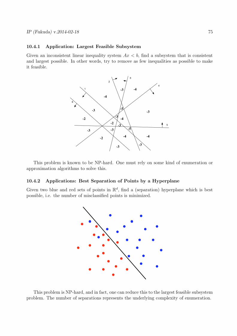
IP (Fukuda) v.2014-02-18 75

10.4.1 Application: Largest Feasible Subsystem

Given an inconsistent linear inequality system Ax < b, find a subsystem that is consistentand largest possible. In other words, try to remove as few inequalities as possible to makeit feasible.

1

2

5

4

3

-4

-3

-3

-2

-2

-3-3

-4

-3

-4-3

-4

-5

-3

-5

6

-3

-4

-3

-2

This problem is known to be NP-hard. One must rely on some kind of enumeration orapproximation algorithms to solve this.

10.4.2 Applications: Best Separation of Points by a Hyperplane

Given two blue and red sets of points in Rd, find a (separation) hyperplane which is bestpossible, i.e. the number of misclassified points is minimized.

This problem is NP-hard, and in fact, one can reduce this to the largest feasible subsystemproblem. The number of separations represents the underlying complexity of enumeration.

IP (Fukuda) v.2014-02-18 76

11 Computing with Arrangements and Zonotopes

As we learned in the previous section that central arrangements of hyperplanes and zono-topes are essentially the same object mathematically. More specifically, if A(A) is a centralarrangement with anm×d representation matrix A, then its face lattice A is anti-isomorphicto the zonotope Z(A) generated by the line segments Li = [−Ai, Ai], j ∈ [m].

This duality implies that one can translate an algorithm for arrangements to an algorithmfor zonotopes. In particular, the following pairs of problems with input matrix A given areequivalent.

Problem 11.1 Cell Enumeration for Arrangements/Vertex Enumeration for Zonotopes

(a) Generating all cells of A(A).

(b) Generating all vertices of Z(A).

Problem 11.2 Vertex Enumeration for Arrangements/Facet Enumeration for Zonotopes

(a) Generating all 1-faces (rays) of A(A).

(b) Generating all facets of Z(A).

Problem 11.3 Face Enumeration for Arrangements/Face Enumeration for Zonotopes

(a) Generating all faces of A(A).

(b) Generating all faces of Z(A).

There is a compact output-polynomial algorithm [5] due to Avis and Fukuda for Problem11.1. Also, there is a worst-case optimal algorithm [20] due to Edelsbrunner, O’Rourke andSeidel for Problem 11.1.

There is a output-polynomial algorithm [49] due to Seymour for Problem 11.2. No com-pact output-polynomial algorithm is known for Problem 11.2. When input is nondegenerate,Problem 11.2 has a trivial algorithm which is compact and output-polynomial, just go thoughall(

m

d−1

)combinations. This suggests that when input is only “slightly” degenerate, the naive

algorithm might be practical.The paper [27] shows that there is an output-polynomial algorithm to generate all faces

of A(A) from the list of cells. This means that together with the compact output-polynomialalgorithm [5] for Problem 11.1, Problem 11.3 can be solved by an output-polynomial algo-rithm.

11.1 Cell Generation for Arrangements

Here we present the reverse search algorithm [5] which is the only compact output-polynomialalgorithm for generating all cells of an arrangement. By duality, this is a compact output-polynomial algorithm for enumerating all vertices of a zonotope.

Let A be an arrangement of distinct hyperplanes hi : i ∈ [m] in Rd, where eachhyperplane is given by a linear equality hi = x : Aix = bi. The two sides of hi are

IP (Fukuda) v.2014-02-18 77

h+i = x : Aix ≥ bi and h−

i = x : Aix ≤ bi. For each x ∈ Rd, the sign vector σ(x) of x isthe vector in −, 0,+m defined by

σ(x)i =

− if x ∈ h−i

0 if x ∈ hi

+ if x ∈ h+i

(i ∈ [m]).

Let VCELL be the set of sign vectors of points in Rd whose nonzero support is [m]. We canidentify each vector c in VCELL with the open cell (open d-face) of the arrangement definedby x : σ(x) = c. For two cells c and c′, let sep(c, c′) be the set of separators of c and c′,that is, the set of elements i in [m] such that ci and c′i have opposite signs. We say that twocells c and c′ are adjacent in GCELL if they differ in only one component, or equivalently,|sep(c, c′)| = 1. The following lemma is important.

Lemma 11.4 For any two distinct cells c and c′ in VCELL, there exists a cell c′′ which isadjacent to c and sep(c, c′′) ⊂ sep(c, c′).

Proof. Let c and c′ be two distinct cells, and let x (x′) be a point in c (in c′, respectively)in general position. Moving from x toward x′ on the line segment [x, x′], we encounter thesequence of cells: co = c, c1, c2, . . . , ck = c′, and we can easily verify that c1 is adjacent to cand sep(c, c1) ⊂ sep(c, c′).

Let us assume that V contains the cell c∗ of all +’s. Lemma 11.4 implies that for each cellc different from c∗, there is a cell c′′ which is adjacent to c and sep(c∗, c′′) ⊂ sep(c∗, c). Letus define fCELL(c) as such c′′ that is lexico-largest (i.e., the unique element in sep(c, c′′) issmallest possible). Then, (GCELL, SCELL, fCELL) is a finite local search with SCELL = c∗.

Figure 11.1 describes the trace of the local search on a small example with d = 2 andm = 4.

By reversing this local search, we obtain an algorithm to list all cells in an arrangement.There are a few things to be explained for an implementation. First, we assumed that thecell c∗ of all +’s is given, but we can pick up any cell c in the arrangement, and consider it asthe cell of all +’s since replacing some equality Aix = bi by −Aix = −bi does not essentiallychange the arrangement. Note that one can obtain an initial cell by picking up any randompoint in Rd and perturbing it if it lies on some hyperplanes.

Now, how can we realize ReverseSearch(AdjCELL,δCELL,SCELL,fCELL) in an efficient way?First we can set δCELL = m and SCELL = c∗. For any cell c ∈ VCELL and k ∈ M , thefunction AdjCELL(c, k) can be realized via solving an LP of the form

minimize (maximize) yksubject to y = Ax− b,

yi ≥ 0 for all i 6= k with ci = +,yi ≤ 0 for all i 6= k with ci = −,

(11.1)

where minimization (maximization) is chosen when ck = + (ck = −, respectively). Thefunction returns the adjacent cell c′ with sep(c, c′) = k if and only if LP (11.1) has afeasible solution with negative (positive) objective value. The time t(AdjCELL) depends onhow an LP with d variables and m − 1 inequalities is solved. We denote this as a functionLP(d,m) of m and d, as we used this notation in Section 8.

IP (Fukuda) v.2014-02-18 78

1

2

3

4

1

2

3

4

++++

+−++

+++−

++−−

++−+

−+−+

−−−+−−++

−−+−

+−+−

Figure 11.1: An arrangement of hyperplanes and the trace of fCELL

There is a straightforward implementation of fCELL, which solves a sequence of LP’ssimilar to (11.1) with objective functions y1, y2, y3, . . .. This means we may have to solveO(m) LP’s in the worst case. Presently we don’t know how to implement it in a moreefficient manner.

Theorem 11.5 There is an implementation of ReverseSearch(AdjCELL, δCELL, SCELL, fCELL)for the cell enumeration problem with time complexity O(m d LP(d,m)|VCELL|) and spacecomplexity O(m d).

Proof. To prove this, first we recall that Theorem 9.2 says, the time complexity ofReverseSearch isO(δ t(Adj)|V |+t(f)|E|). As we remarked earlier, δCELL = m, t(AdjCELL) =O(LP(d,m)), and t(fCELL) = O(m LP(d,m)). Since |ECELL| ≤ d |VCELL| holds for anyarrangement (see [27]), the claimed time complexity follows. The space complexity is clearlysame as the input size O(m d).

IP (Fukuda) v.2014-02-18 79

12 Minkowski Additions of Polytopes

A zonotope is a very special Minkowski sum of polytopes, namely, a Minkowski of linesegments. In this section, we study the complexity of Minkowski sums of polytopes P1, . . .,Pk in Rd and some algorithms for computing Minkowski sums of polytopes.

+ =

There are three basic variations of the problem. When input is H-polytopes and output isalso H-polytope, Tiwary [50] has recently proved that the associated decision problem is NP-hard for k = 2. Here the associated decision problem is to test whether a given H-polytopeP is the Minkowski sum of given H-polytopes P1, . . ., Pk. When input is V-polytopes andoutput is H-polytope, the problem contains the representation conversion for polytopes as aspecial case (k = 1) whose complexity is still unknown. The last case when both input andoutput are V-polytopes is the only case for which an output-polynomial algorithm is known.

In this section, we present a compact output-polynomial algorithm for the last case. Thealgorithm is a natural extension of (the dual form of) the reverse search algorithm given inSection 11.1.

Faces, Minkowski Decomposition and Adjacency

For a polytope P and for any vector c ∈ Rd, the set of maximizers x of the inner productcTx over P is denoted by S(P ; c). Thus each nonempty face of P is S(P ; c) for some c.We denote by F (P ) the set of faces of P , by Fi(P ) the set of i-dimensional faces, and byfi(P ) the number of i-dimensional faces, for i = −1, 0, . . . , d, For each nonempty face F ,the relatively open polyhedral cone of outer normals of P at F is denoted by N (F ;P ).Thus, c ∈ N (F ;P ) if and only if F = S(P ; c). The normal fan N (P ) of P is the cellcomplex N (F ;P )|F ∈ F (P ) whose body is Rd. If F is i-dimensional (i = 0, 1, . . . , d), thenormal cone N (F ;P ) is (d− i)-dimensional. Thus the extreme points of P are in one-to-onecorrespondence with the full dimensional faces (which we call the regions or cells) of thecomplex.

Proposition 12.1 Let P1, P2, ..., Pk be polytopes in Rd and let P = P1 + P2 + · · · + Pk.Then a nonempty subset F of P is a face of P if and only if F = F1+F2+ · · ·+Fk for someface Fi of Pi such that there exists c ∈ Rd (not depending on i) with Fi = S(Pi; c) for all i.Furthermore, the decomposition F = F1 + F2 + · · ·+ Fk of any nonempty face F is unique.

Proof. The equivalence follows directly from the obvious relation [30, Lemma 2.1.4]

S(P1 + P2 + · · ·+ Pk; c) = S(P1; c) + S(P2; c) + · · ·+ S(Pk; c) for any c ∈ Rd.

IP (Fukuda) v.2014-02-18 80

For the uniqueness, let F be a nonempty face with F = S(P ; c) for some c and let F =F1 + F2 + · · · + Fk be any decomposition. First, note that Fi ⊆ S(P;c) for all i, becausethe value cTx for any x ∈ F is the sum of the maximum values cTxi subject to xi ∈ Pi fori = 1, . . . , k, and thus if x ∈ F and x = x1 + x2 + · · · + xk for xi ∈ Fi, then xi ∈ S(Pi, c).Now suppose there exists Fi properly contained in S(Pi; c). Let v be an extreme point ofS(Pi; c) not in Fi. Then there is a linear function wTx such that wTv is strictly greater thanany value attained by x ∈ Fi. Now let x∗ be any point attaining the maximum of wTx overthe polytope F1 + F2 + · · ·Fi−1 + Fi+1 + · · ·+ Fk. Clearly x∗ + v ∈ F but this point cannotbe in F1 + F2 + · · ·+ Fk, a contradiction. This proves the uniqueness.

We refer the unique decomposition F = F1 + F2 + · · ·+ Fk of a nonempty face F as theMinkowski decomposition. Here, the dimension of F is at least as large as the dimension ofeach Fi. Thus we have the following.

Corollary 12.2 Let P1, P2, ..., Pk be polytopes in Rd and let P = P1 + P2 + · · · + Pk. Avector v ∈ P is an extreme point of P if and only if v = v1 + v2 + · · ·+ vk for some extremepoint vi of Pi and there exists c ∈ Rd with vi = S(Pi; c) for all i.

For our algorithm to be presented in the next section, it is important to characterize theadjacency of extreme points in P .

Corollary 12.3 Let P1, P2, ..., Pk be polytopes in Rd and let P = P1 + P2 + · · · + Pk. Asubset E of P is an edge of P if and only if E = E1 +E2 + · · ·+Ek for some face Ei of Pi

such that dim(Ei) = 0 or 1 for each i and all faces Ei of dimension 1 are parallel, and thereexists c ∈ Rd with Ei = S(Pi; c) for all i.

The following variation of the above is useful for the algorithm to be presented. Theessential meaning is that the adjacency of extreme points is inherited from those of Minkowskisummands.

Proposition 12.4 Let P1, P2, ..., Pk be polytopes in Rd and let P = P1 + P2 + · · · + Pk.Let u and v be adjacent extreme points of P with the Minkowski decompositions: u = u1 +u2 + · · ·+ uk and v = v1 + v2 + · · ·+ vk. Then ui and vi are either equal or adjacent in Pi

for each i.

Proof. Let u and v be adjacent extreme points. It is sufficient to show that [u, v] =[u1, v1] + [u2, v2] + · · · + [uk, vk] and each [ui, vi] is a face of Pi. Let c ∈ Rd be such that[u, v] = S(P ; c). Because [u, v] = S(P1; c) + S(P2; c) + · · ·+ S(Pk; c) and by the uniquenessof decomposition of u and v, both uj and vj are in S(Pj, c), for all j. This implies that[uj, vj] ⊆ S(Pj, c), for all j. On the other hand, one can easily see that in general [u, v] ⊆[u1, v1] + [u2, v2] + · · ·+ [uk, vk]. The last two relations give [uj, vj] = S(Pj , c) for all j. Thiscompletes the proof.

This proposition immediately provides a polynomial algorithm for listing all neighborsof a given extreme point using linear programming.

IP (Fukuda) v.2014-02-18 81

12.1 Complexity of Minskowski Sums of V-Polytopes

The nontriviality of computing Minkowski sums of V-polytopes can be understood by howthe complexity of Minkowski sums varies from some instances to another. In particular, weare most concerned with the complexity of sums in terms of the size of summands.

The first proposition shows that the vertex complexity of Minknowski sums is linearlybounded by the vertex complexity of summand polytopes.

Proposition 12.5 (Linearly Bounded Minkowski-Addition) . For each k ≥ 2 andd ≥ 2, there is an infinite family of Minkowski additions for which f0(P1 + P2 + · · ·+ Pk) ≤f0(P1) + f0(P2) + · · ·+ f0(Pk).

Proof. Suppose k ≥ 2 and d ≥ 2. First pick up any d-polytope, say Q, with at least kextreme points, and select k extreme points. For each jth selected extreme point vj, make anew polytope Pj from Q by truncating only vj with one or more hyperplanes. Now we claimthat the number f0(P1 + P2 + · · · + Pk) ≤ f0(P1) + f0(P2) + · · · + f0(Pk). See Figure 12.1for an example for k = 2, d = 3 and Q is a 3-cube. To see this, let v be an extreme point ofPj for some fixed j. There are three cases. The first case is when v is an unselected one, i.e.an extreme point of Q not selected. In this case, it can be an Minkowski summand of anextreme point of P in a unique way, since any linear function maximized exactly at v overPj is maximized exactly at v over other Pi’s. The second case is when v is a newly createdvertex by the truncation of vj. Since it is obtained by the truncation of vj , any linear functionmaximized exactly at v over Pj is maximized exactly at vj over other other Pi’s. The lastcase is when v = vi for some i 6= j. This case is essentially the same as the second casewhere v contributes uniquely to a new extreme point with each truncation vertex of Pi. ByCorollary 12.2, every extreme point of Pj contributes at most once to f0(P1+P2+ · · ·+Pk).This completes the proof.

+ =

Figure 12.1: Minkowski Sum of Truncated Cubes

The following theorem gives the other extreme to the previous proposition. Namely, theobvious upper bound of the vertex complexity can be achieved for a large class of Minkowskisums of polytopes.

IP (Fukuda) v.2014-02-18 82

Theorem 12.6 (Tight Upper Bound [28]) .In dimension d ≥ 3, it is possible to choose k (≤ d − 1) polytopes P1, . . . , Pk so that thetrivial upper bound for the number of vertices is attained by their Minkowski sum.

f0(P1 + P2 + · · ·+ Pk) = f0(P1)× f0(P2)× · · · × f0(Pk).

Proof. Here we give outline only, see [28] for a precise construction. On k (≤ d − 1)orthogonal planes in Rd, place vi points in convex position. Perturb the points slightly tomake each Pi full dimensional. Figure 12.2 shows the case when f0(P1) = f0(P2) = 4 andf0(P ) = f0(P1)× f0(P2) = 16

+ =

Figure 12.2: Minkowski Sum of (d− 1) Thin Polytopes in Orthogonal Spaces

12.2 Extension of a Zonotope Construction Algorithm

We assume in this section that P1, P2, ..., Pk are polytopes in Rd given by the sets V1,V2, ..., Vk of extreme points. We also assume that the graph G(Pj) of Pj is given by theadjacency list (Adjj(v, i) : i = 1, . . . , δj) of vertices adjacent to vertex v ∈ Vj in graph G(Pj),where δj is the maximum degree of G(Pj) for each j = 1, . . . , k. If the degree degj(v) ofv is less than δj in G(Pj), we assume that Adjj(v, i) = null for all i > degj(v). Finallywe define δ = δ1 + δ2 + · · · + δk, an upper bound of the maximum degree of G(P ), due toProposition 12.4. For example, when the input polytopes are simple and full dimensionalthen δj = d for all j and δ = k d. Note that for a given set Vj, one can compute the adjacencylist in polynomial time using linear programming.

Recall that the Minkowski addition problem is to compute the set V of extreme points ofP = P1+P2+ · · ·+Pk. We shall present a compact polynomial algorithm for the Minkowskiaddition problem.

The key idea in our algorithm design

The main algorithmic idea is quite simple. Just like for the vertex enumeration for convexpolyhedra using reverse search given in Section 9.2, it traces a directed spanning tree T ofthe graph G(P ) of P rooted at an initial extreme point v∗. The difference from the vertexenumeration algorithm is that the polytope P is not given by a system of inequalities (i.e.not an H-polytope) in the present setting but as a Minkowski-addition of V-polytopes. Thus

IP (Fukuda) v.2014-02-18 83

we need to introduce a new way of defining a directed spanning tree that is easy to trace.We shall use the following simple geometric property of normal fans.

Proposition 12.7 Let v and v′ be two distinct extreme points of P , and let c ∈ N (v;P )and c′ ∈ N (v′;P ). Then there exists an extreme point v′′ adjacent to v such that N (v′′;P )contains a point of form (1− θ)c + θc′ for some 0 ≤ θ ≤ 1.

Proof. Since v 6= v′, their outer normal cones are two distinct full dimensional conesin the normal fan N (P ). This means that the parameterized point t(θ) := c + θ(c′ − c)(0 ≤ θ ≤ 1) in the line segment [c, c′] must leave at least one of the bounding halfspaces ofthe first cone N (v;P ) as θ increases from 0 to 1. Since the bounding halfspaces of N (v;P )are in one-to-one correspondence with the edges of G incident to v, any one of the halfspacesviolated first corresponds to a vertex v′′ adjacent to v claimed by the proposition.

Let us fix v∗ as an initial extreme point of P . Finding one extreme point of P is easy.Just select any generic c ∈ Rd, and find the unique maximizer extreme point vi of cTx overPi, for each i. The point v = v1 + v2 + · · ·+ vk is an extreme point of P .

Now we construct a directed spanning tree of G(P ) rooted at v∗ as follows. Let v ∈ Vbe any vertex different from v∗. We assume for the moment that there is some canonicalway to select an interior point of the normal cone of P at any given vertex, as we shall giveone method to determine such a point later. Let c and c∗ be the canonical vector of N (v;P )and N (v∗;P ), respectively. By Proposition 12.7, by setting v′ = v∗, we know that thereis a vertex v′′ adjacent to v such that N (v′′;P ) meets the segment [c, c∗]. In general theremight be several such vertices v′′ (degeneracy). We break ties by the standard symbolicperturbation of c as c + (ǫ1, ǫ2, . . . , ǫd)T for sufficiently small ǫ > 0. Define the mappingf : V \ v∗ → V as f(v) = v′′. This mapping, called a local search function in reversesearch, determines the directed spanning tree T (f) = (V,E(f)) rooted at v∗, where E(f) isthe set of directed edges (v, f(v))|v ∈ V \ v∗.

Proposition 12.8 The digraph T (f) is a spanning tree of G(P ) (as undirected graph) andv∗ is a unique sink node of T (f).

Proof. By the construction, v∗ is a unique sink node of T (f). It is sufficient to show thatT (f) has no directed cycle. For this, take any edge (v, v′′ = f(v)) ∈ E(f). Let c, c∗ be thecanonical vector for v, v∗, respectively. Without loss of generality, we assume nondegeneracy,since one can replace c with the perturbed vector c + (ǫ1, ǫ2, . . . , ǫd)T . Since c is an interiorpoint of N (v;P ),

cT (v − v′′) > 0. (12.1)

Again, by the construction and because the canonical points are selected as interior points ofthe associated normal cones, there exists 0 < θ < 1 such that c := (1− θ)c+ θc∗ ∈ N (v′′;P ).This implies cT (v′′ − v) > 0, that is,

0 < ((1− θ)c + θc∗)T (v′′ − v)

= (1− θ)cT (v′′ − v) + θ(c∗)T (v′′ − v)

< θ(c∗)T (v′′ − v) ( by (12.1) ) .

IP (Fukuda) v.2014-02-18 84

This implies that the vertex v′′ attains a strictly higher inner product with c∗ than v. There-fore, there is no directed cycle in T (f).

Figure 12.3 shows an example of the directed spanning tree T (f) in green.

v* v*

Figure 12.3: The Graph G(P ) and A Rooted Spanning Tree T (f)

A reverse search algorithm, to be presented below, traces reversely the tree from the rootv∗ in depth-first manner, using an adjacency oracle.

The critical computation in our algorithm is solving a linear programming problem. Wedenote by LP(d,m) the time, as we used in Section 8. necessary to solve a linear programmingin d variables and m inequalities.

Now we can state the complexity of our algorithm.

Theorem 12.9 There is a compact polynomial algorithm for the Minkowski addition of kpolytopes that runs in time O(δ LP(d, δ)f0(P )) and space linear in the input size.

The algorithm

The sequel of the section is devoted to present the technical details of a reverse searchalgorithm that traces T (f) starting from its root vertex v∗ against the orientation of edges.We shall prove Theorem 12.9 at the end.

As usual, our reverse search algorithm requires, in addition to the local search functionf , an adjacency oracle function that implicitly determines the graph G(P ).

Let v be any vertex of P with the Minkowski decomposition v = v1 + v2 + · · ·+ vk (see,Corollary ??). Let

∆ = (j, i) : j = 1, . . . , k and i = 1, . . . , δj. (12.2)

Recall that for any (j, i) ∈ ∆, Adjj(vj, i) is the ith vertex adjacent to vj whenever it is notnull . We shall call a pair (j, i) valid for v if Adjj(vj , i) 6= null , and invalid otherwise. Letus define the associated edge vectors ej (vj , i) by

ej (vj , i) =

Adjj(vj, i)− vj (j, i) is valid for v

null otherwise.(12.3)

IP (Fukuda) v.2014-02-18 85

Proposition 12.4 shows that all edges of P incident to v are coming from the edges incidentto vj ’s, or more precisely, each edge of P incident to v is parallel to some ej (vj , i). Thisimmediately implies that δ is an obvious upper bound of the degree of v. For each (s, r) ∈ ∆,let us group the same (parallel) directions together as

∆(v, s, r) = (j, i) ∈ ∆ : ej (vj , i) ‖ es(vs , r). (12.4)

Consider it as the empty set if (s, r) is invalid. Now, for any given pair (s, r) ∈ ∆, checkingwhether es(vs , r) determines an edge direction of P is easily reducible to an LP (or moreprecisely, a linear feasibility problem):

es(vs , r)Tλ < 0,

ej (vj , i)Tλ ≥ 0 for all valid (j, i) 6∈ ∆(v, s, r).

(12.5)

More precisely, the system (12.5) has a solution λ if and only if the direction es(vs , r)determines an edge of P incident to v. If it has a feasible solution, then by Proposition 12.4,the vertex v adjacent to v along this direction is given by

v = v1 + v2 + · · ·+ vk

vj =

Adjj(vj , i) if there exists i such that (j, i) ∈ ∆(v, s, r)

vj otherwise.

Let us denote by ∆(v) as the set of all pairs (s, r) ∈ ∆ such that es(vs , r) determines an edgeof P and (s, r) is a member of ∆(v, s, r) with the smallest first index. This set represents aduplication-free index set of all edge directions at v.

Now we are ready to define our adjacency oracle as a function Adj : V ×∆ → V ∪nullsuch that

Adj(v, (s, r)) =

v if (s, r) ∈ ∆(v)

null otherwise.(12.6)

Lemma 12.10 One can evaluate the adjacency oracle Adj(v, (s, r)) in time LP(d, δ).

Proof. The essential part of the evaluation is solving the system (12.5). Since δ = |∆|,the system has d variables and at most δ inequalities and the claim follows.

Lemma 12.11 There is an implementation of the local search function f(v) with evaluationtime O(LP(d, δ)), for each v ∈ V \v∗ with the Minkowski decomposition v = v1+v2+· · ·+vk.

Proof. The implementation of f essentially depends on how we define the canonicalvector of the normal cone N (v;P ). Like in the adjacency oracle implementation, we usean LP formulation. Since the set of directions ej (v , i) for valid (j, i) ∈ ∆ include all edgedirections at v, the normal cone N (v;P ) is the set of solutions λ to the system

ej (vj , i)Tλ ≤ 0 for all valid (j, i) ∈ ∆.

Since we need an interior point of the cone, we formulate the following LP:

max λ0

subject toej (vj , i)

Tλ + λ0 ≤ 0 for all valid (j, i) ∈ ∆λ0 ≤ K.

(12.7)

IP (Fukuda) v.2014-02-18 86

HereK is any positive constant. Since v is a vertex of P , this LP has an optimal solution. Westill need to define a unique optimal solution. For this, we use a very pragmatic definition: fixone deterministic algorithm and define the canonical vector as the unique solution returnedby the algorithm. Since the number of variables is d + 1 and the number of inequalities isat most δ + 1, the assumptions on LP implies the time complexity O(LP(d, δ)) to computethe canonical vector. Note that for practical purposes, we should probably add boundinginequalities for λ to the LP (12.7) such as −1 ≤ λi ≤ 1 for all i to make sure that the optimalsolution stays in a reasonable range. This does not change the complexity.

An execution of f requires to compute the canonical vectors c and c∗. Once they arecomputed, the remaining part is to determine the first bounding hyperplane of the normalcone N (v;P ) hit by the oriented line t(θ) := c+ θ(c∗ − c) (as θ increases from 0 to 1). Thisamounts to solving at most δ one-variable equations, and is dominated by the canonicalvector computation.

In Figure 12.4, we present the resulting reverse search algorithm, where we assume thatthe δ index pairs (j, i) in ∆ are ordered as (1, 1) < (1, 2) < · · · < (1, δ1) < (2, 1) < · · · <(k, δk).

procedure MinkowskiAddition(Adj,(δ1, . . . , δk), v∗,f);

v := v∗; (j, i) := (1, 0); (* (j, i): neighbor counter *)output v;repeat

while (j, i) < (k, δk) doincrement (j, i) by one;

(r1) next := Adj(v, (j, i));if next 6= null then

(r2) if f(next) = v then (* reverse traverse *)v := next;(j, i) := (1, 0);output v

endifendif

endwhile;if v 6= v∗ then (* forward traverse *)

(f1) u := v; v := f(v);(f2) restore (j, i) such that Adj(v, (j, i)) = u

endifuntil v = v∗ and (j, i) = (k, δk).

Figure 12.4: Reverse Search Algorithm for Minkowski Sum

Finally, we are ready to prove the main theorem, Theorem 12.9.

Proof. We use the general complexity result, Corollary 9.3, saying the time complexityof the reverse search in Figure 12.4 is O(δ(t(Adj) + t(f))|V |). By Lemma 12.10 and Lemma12.11, both t(Adj) and t(f) can be replaced by LP(d, δ). Since f0(P ) = |V |, the claimed

IP (Fukuda) v.2014-02-18 87

time complexity follows. The space complexity is dominated by those of the functions f andAdj which are clearly linear in the input size.

IP (Fukuda) v.2014-02-18 88

13 Problem Reductions in Polyhedral Computation

In this section, we look at some basic problems in polyhedral computation. Just like incombinatorial optimization, it is quite hard to distinguish hard problems (typically NP-hardproblems) from easy problems. Here there are two sorts of easy problems. The first groupconsists of decision problems that are polynomially solvable. The second group consists ofenumeration problems that may require output whose size is exponential in the input size,but are output-polynomially solvable.

We shall present some hard decision problems in Section 13.1, and discuss some hardenumeration problems in Section 13.2.

13.1 Hard Decision Problems in Polyhedral Computation

We start with two decision problems in polyhedral computation that are related to linearprogramming but are known to be hard.

For A ∈ Qm×d and b ∈ Qm, let PH(A, b) be the H-polyhedron

PH(A, b) := x ∈ Rd : Ax ≤ b, (13.1)

and let A(A, b) be the associated arrangement of hyperplanes:

A(A, b) := h1, . . . , hm, (13.2)

hi := x ∈ Rd : Aix ≤ bi. (13.3)

Problem 13.1 Optimal Vertex of a Polyhedron (OVP)

• Input: A ∈ Qm×d, b ∈ Qm, c ∈ Qd and K ∈ Q.

• Question: Does there exists a vertex v of PH(A, b) with cTv ≥ K?

Problem 13.2 K-Vertex of a Polyhedron (KVP


• Question: Does there exists a vertex v of PH(A, b) with cTv = K?

Theorem 13.3 ([26]) The decision problems OVP and KVP are both NP-complete.

Proof. It is clear that both problems are in the class NP. The proofs of the NP-completeness will be obtained by a polynomial time transformation from the following prob-lem, known to be NP-complete in the strong sense [29]:

Problem 13.4 Directed Hamiltonian Path (DHP)

• Input: A directed graph G = (V,A) and two distinct vertices s, t ∈ V .

• Question: Does G contain a directed Hamiltonian path from s to t ?

IP (Fukuda) v.2014-02-18 89

Let G = (V,A) be a directed graph and s 6= t ∈ V . Associate a variable xij with eacharc (i, j) ∈ A. Let P (G) be the polytope given by:

∑

j|(i,j)∈Axij −

∑

j|(j,i)∈Axji = 0, for each i ∈ V − s, t, (13.4)

∑

j|(s,j)∈Axsj −

∑

j|(j,s)∈Axjs = 1, (13.5)

∑

j|(t,j)∈Axtj −

∑

j|(j,t)∈Axjt = −1, (13.6)

xij ≥ 0, for each (i, j) ∈ A. (13.7)

The matrix of the coefficients of these inequalities is totally unimodular ([43], Proposition2.6, p. 542) implying that P (G) is integral. It follows that an extreme point x of P (G) isthe characteristic vector of a directed path joining s to t in G and, possibly, a set of circuits.If a circuit C exists, then x is a convex combination of the two points obtained by addingor subtracting small ǫ > 0 on all the arcs of the circuit, a contradiction. Hence x is thecharacteristic vector of a simple directed path joining s to t. One verify easily that all suchpaths are extreme points of P (G), proving that the extreme points of P (G) are exactly thecharacteristic vectors of the simple directed paths joining s to t in G. These two facts thusimply that, for K = |V | − 1 and c = 1 (the vector of all 1’s), both the OVP and the KVPproblems for P (G) are NP-complete in the strong sense. This completes the proof.

There are similar complexity results for arrangements of hyperplanes.

Problem 13.5 Optimal Vertex of an Arrangement (OVA)


• Question: Does there exists a vertex v of A(A, b) with cTv ≥ K?

Problem 13.6 Optimal Vertex of an Arrangement (KVA)


• Question: Does there exists a vertex v of A(A, b) with cTv = K?

Theorem 13.7 ([26]) The decision problems OVA and KVA are both NP-complete.

Proof. Consider an instance of DHP and build a corresponding instance for OVA andKVA as follows: To each arc (i, j) ∈ A, we associate a variable xij . Let d := |A|, K := |V |−1,c = 1 and define the arrangement generated by the following set of hyperplanes:

IP (Fukuda) v.2014-02-18 90

Hi := x ∈ Rd|∑

j|(i,j)∈Axij −

∑

j|(j,i)∈Axji = 0, for each i ∈ V − s, t, (13.8)

Hs := x ∈ Rd|∑

j|(s,j)∈Axsj −

∑

j|(j,s)∈Axjs = 1, (13.9)

Ht := x ∈ Rd|∑

j|(t,j)∈Axtj −

∑

j|(j,t)∈Axjt = −1, (13.10)

Hij := x ∈ Rd| xij = 0, for each (i, j) ∈ A. (13.11)

First we observe that if DHP has a “yes” answer, so does the corresponding instance ofOVA and KVA, as the characteristic vector of any directed Hamiltonian path lies on the |V |hyperplanes Hi for i ∈ V as well as on (|A|−(|V |−1)) = |A|−|V |+1 of the hyperplanes Hij

for i 6= j ∈ V . Note that the |V | hyperplanes Hi for i ∈ V are not linearly independent, butany subset of (|V |−1) of them are. Hence there are (|A|− |V |+1)+ (|V |−1) = |A| linearlyindependent hyperplanes containing the characteristic vector of any directed Hamiltonianpath joining s to t in G, implying that the latter is a vertex of the given arrangement.

Now suppose that KVA or OVA has a “yes” answer produced by a vertex v of the con-structed instance. One can write the |A| equations defining the hyperplanes of the instanceas a system of the form Ax = b. It is well known that the matrix [A, b] is totally unimodular(see [43] for example). Thus any vertex of the arrangement has only +1,−1, or 0 coordinates,as shown by Cramer’s rule for solving a linear system.

Let S be a set of n linearly independent hyperplanes of the given family whose intersectionis v. As the |V | hyperplanes in Hi|i ∈ V are not linearly independent, the number of thesehyperplanes which are in S is at most (|V | − 1). Hence the number of non zero coordinatesof v is at most (|V | − 1). As c = 1 and cTv ≥ K = (|V | − 1), we have that exactly (|V | − 1)coordinates of v are (+1), all the others being (0)’s. Thus v is the characteristic vector of aset P of (|V | − 1) arcs of A. This also implies that KVA has a “yes” answer if and only ifOVA has a “yes” answer

If P is a directed Hamiltonian path in G joining s to t, then we are done. Otherwise, Pcontains a directed path joining s to t in G and at least one directed cycle C. But considerv′ ∈ Rn defined by

v′ij =

0 if (i, j) ∈ C,vij otherwise,

for each (i, j) ∈ A. (13.12)

This complete the proof.

IP (Fukuda) v.2014-02-18 91

13.2 Hard Enumeration Problems in Polyhedral Computation

For matrices V ∈ Qs×d and R ∈ Qt×d, the V-polyhedron with representation pair (V,R) isdenoted by PV (V,R), i.e.,

PV (V,R) := x : x = V λ +Rµ, 1Tλ = 1, λ ≥ 0, µ ≥ 0. (13.13)

The following decision problem is arguably the most important problem in polyhedralcomputation.

Problem 13.8 Polyhedral Verification Problem (PVP)

• Input: A ∈ Qm×d, b ∈ Qm, V ∈ Qs×d and R ∈ Qt×d.

• Question: Is PH(A, b) 6= PV (V,R) ?

It is not difficult to prove that if PVP is in P, then there is an output-polynomial algorithmfor the polyhedral representation conversion problem discussed in Section 9, see PolyhedralComputation FAQ [23].

PVP is easily seen to be in NP, because if the polyhedra are not equal, there is a succinctcertificate for it, a point x in one of the polyhedra which is not in the other. Unfortunately,the complexity of PVP is still open. The decision problem PVP was first posed by Lovasz,see [49], and has been extensively studied by many researchers.

One of the most exciting progresses is the NP-completeness of a closely related problem,due to Khachiyan et al. [35].

Problem 13.9 Vertex Enumeration for an Unbounded Polyhedron (VEU)

• Input: A ∈ Qm×d, b ∈ Qm and V ∈ Qs×d.

• Question: Does the H-polyhedron PH(A, b) contain a vertex not in V ?

Theorem 13.10 ([26]) The decision problems VEU is NP-complete.

Proof. (Outline) It is easily seen to be in NP, because if the answer is yes, then there isat least one vertex not in V . The proof uses a reduction from the NP-complete problem:

Problem 13.11 Negative Circuit Enumeration (NCE)

• Input: A digraph G = (V,E) with edge weight w : E → Q, and a family S of negativecircuits of G.

• Question: Does G contain a negative circuit not in the family S?

Here, a negative circuit is a directed circuit C ⊂ E whose total weight∑

e∈C is negative. Itis shown by Khachiyan et al. [35] that NCE is NP-complete from a reduction from SAT.

(This section is to be extended.)

IP (Fukuda) v.2014-02-18 92

14 Evolutions and Applications of Polyhedral Compu-

tation

Polyhedral Computation has been shaped and polished through actual demands from nu-merous mathematicians, scientists, engineers and even social scientists. In this section, wepresent the author’s personal involvements in various external or internal projects whichhave driven the advancement of polyhedral computation and software developments.

1987 – 1992: The First Stage. The first generation of codes for polyhedral representa-tion conversion were written first for mathematicians to understand certain combina-torial polyhedra, such as cut polytopes, cut cones, and traveling salesman poly-topes. It is extremely difficult to determine the facet inequalities of these polyhedrabecause typical associated combinatorial optimization problems are NP-hard. How-ever, by computing the H-representation from a V-representation for small instances,many new facet inequalities were discovered and used for finding a stronger LP relax-ation of NP-hard optimization problems. The first version of my implementation ofthe double description algorithm described in Section 9.1 was released in January 1988is called pdd where p stands for the programming language Pascal. It helped the earlystage of research on cut polytopes by Michel Deza and Monique Laurent, see [17, 18].

1993 – 1996: The Critical Second Stage. Then, a more computationally demandingtask was needed for research in material science. Two physicists G. Ceder andG.D. Garbulsky at MIT contacted both David Avis and myself in 1993, and askedfor our computational help in enumerating all extreme points of a highly degeneratepolytope in dimension 8 given by 729 inequalities. The vertices represent physicallystable states of a ternary (3 elements) alloy. David had a C-implementation namedrs (which was replaced by lrs later) of the reverse search algorithm given in Section9.2 then, and I had a C-version named cdd of the earlier code pdd. Both David andmyself devoted our effort to compute the vertices, and finally it took us about a monthto compute the results. Our greatest excitement came when we verified that the finalresults computed by our implementations of two totally different algorithms returnedexactly the same results. This successful computation lead to a paper by the four ofus [12].

About the same time, then a doctoral student Francisco Valero of neuromuscularsystems laboratory at Stanford University contacted me. The application Valerodiscovered then surprised me considerably. I did not imagine that one can find anapplication of polyhedral computation in human bodies and muscles. He email in May1994 describing his application reads

My application deals with finger muscles having force limits (i.e., formzero force to their maximum physiological force for each finger muscle) whichdefines a hypercube in a dimension equal to the number of muscles underconsideration. Other mechanical, functional or anatomical characteristicsproduce further constrain equations (i.e., need the force of the finger to bezero in certain directions, finger size/configuration, etc.). The vertex enu-meration technique helps me identify the limits of muscle force production

IP (Fukuda) v.2014-02-18 93

under these constraints, which in turn maps into functional limits such asmaximum finger forces, accelerations, etc, which are independent of muscleforce coordination. Coordination can be studied with standard linear pro-gramming techniques. The limits of function, however, require the explicitenumeration of the vertices of convex polyhedra in n-dimensional space.

Valero has been a strong advocate of computational geometry techniques applied tobiomedical and biomechanics fields since then. A recent paper [36] shows the anal-ysis of muscle redundancies using the vertex enumeration in polyhedra.

From the software development front, a new C++ version of cdd, called cdd+, wasreleased in April 1995 which has the capability of using both floating-point and rationalexact arithmetic using GMP [1].

1997 – 2007: Developments of Polyhedral Computation Libraries. Further advance-ments were made during this period for the development of software C-libraries cddliband lrslib, based on cdd and lrs, respectively by Fukuda [22] and Avis [2]. Natu-rally, these libraries have been integrated into other programs.

A versatile R-interface of cddlib was written by the statistician Charles Geyer ofUniversity of Minnesota. It is available from

http://www.stat.umn.edu/˜charlie/

A webpage of computing all Nash equilibria of bimatrix games using lrslib writtenby Rahul Savani became available at

http://banach.lse.ac.uk/form.html.

A Matlab toolbox for the study of control theory with an emphasis on parametricoptimization was written by a group of researchers at the system dynamics and controlgroup at ETH Zurich. It has an interface called cddmex to cddlib and is available at

http://control.ee.ethz.ch/research/software.en.html

A Python interface PyPolyhedron to cddlib was written by Pearu Peterson. Hewrote in his email in 2007 “I am using it for analyzing multi-soliton interactions. Interms of computational geometry, I just construct special polyhedron in (N + 1)-Dspace, project it to N -D space, and then find its intersection with 2-D hyperplane,which after projecting to 2-D space gives an interaction pattern of the N -soliton solu-tion.” It is available at http://cens.ioc.ee/projects/polyhedron/

Polymake is a platform to do polyhedral and algebraic computation mainly formathematicians whose two core engines are cddlib and lrslib. It is available athttp://www.polymake.org/doku.php

TOPCOM [45] is a package for computing Triangulations Of Point Configurationsand Oriented Matroids. It uses the LP code of cddlib for the recognition of regulartriangulations.

Minksum [http://www.cs.dartmouth.edu/˜weibel/minksum.php] is a program to com-pute the V-representation (i.e. the set of vertices) of the Minkowski addition of severalconvex polytopes given by their V-representation. It is an implementation in C++

http://www.stat.umn.edu/~charlie/

http://banach.lse.ac.uk/form.html

http://control.ee.ethz.ch/research/software.en.html

http://cens.ioc.ee/projects/polyhedron/

http://www.polymake.org/doku.php

http://www.cs.dartmouth.edu/~weibel/minksum.php

IP (Fukuda) v.2014-02-18 94

language of the reverse search algorithm given in Section 12.2 whose time complexityis polynomially bounded by the sizes of input and output. It relies on the exact LPsolver of cddlib.

Gfan [33] is a program to list all reduced Grobner bases of a general polynomialideal given by a set of generating polynomials in -variables. It is an implementation inC++ language of the reverse search algorithm [25]. It relies on the exact LP solver ofcddlib.

2004 – 2011: Expanding Application Fields. An application of Minkowski sum ofpolytopes presented in Section 12 is given in a doctoral thesis of J.P. Petit [44] in2004, which is computer aided tolerancing in design and manufacturing usinga mathematical model with convex polytopes in dimension 6. The dimension is simply3 + 3 where the first 3 is the dimension of the space and the latter is the freedom ofmovement in 3-space.

A polyhedral model was introduced in a doctoral research at Queen’s University Belfastguided by Cecil Armstrong on aircraft stress load evaluation and optimization.The essential problem is to detect the most critical parts of aircrafts against a set ofmany likely stresses, which is reduced to the redundancy removal in linear inequalitysystems, the theme of Section 8.2.

To analyze the effects of United Nations peacekeeping operations, the dangerof using the high dimensional analysis is pointed out in a paper by political scientistsin [46], after a few researchers in computational geometry including myself presentedcounter-intuitive facts in higher dimensional spaces. In particular, one serious problemof estimating the effect of a future operation, a relatively small set of past instancesrepresented by high dimensional points cannot be a reliable guidance, due to the factthat a new point will most likely be (far) outside of the convex hull of the pastdata points, and thus a wild extrapolation occurs at a high probability.

Future. From my personal involvements in polyhedral computation during the past 24years, once reliable and efficient codes of polyhedral computation become available,new users might show up from any field of science, engineering, humanities and evenarts. Thus, the main purpose of writing this book is to present the fundamental theoryof polyhedra and the basic computational problems associated polyhedra with mostefficient algorithmic techniques. My belief is that interesting applications should followonce researchers have easy access to the theory and computational codes. After all,convex polyhedra appear almost everywhere, implicitly or explicitly.

IP (Fukuda) v.2014-02-18 95

15 Literatures and Software

Course materials will be distributed as pdf files from our course webpage.For the theory of linear programming, recommended sources are [47, 14, 24]. Some of the

excellent books on combinatorial optimization are [16, 31, 48]. There are excellent books onconvex polyhedra, see [39, 32, 51]. For good discussions on algorithmic and combinatorialaspects of polyhedra, see [41, 37, 34]. The standard text on oriented matroids is [9], and anexcellent introduction is included in the dissertation [21] which is available online.

We use some of the freely available software packages such as lrslib [2] and cddlib [22]for polyhedral representation conversion.

References

[1] GMP, GNU’s library for arbitrary precision arithmetic. http://gmplib.org/.

[2] D. Avis. lrs homepage. McGill University. http://cgm.cs.mcgill.ca/˜avis/C/lrs.html.

[3] D. Avis, D. Bremner, and R. Seidel. How good are convex hull algorithms. Computa-tional Geometry: Theory and Applications, 7:265–302, 1997.

[4] D. Avis and K. Fukuda. A pivoting algorithm for convex hulls and vertex enumerationof arrangements and polyhedra. Discrete Comput. Geom., 8:295–313, 1992.

[5] D. Avis and K. Fukuda. Reverse search for enumeration. Discrete Applied Mathematics,65:21–46, 1996.

[6] M. Balinski. An algorithm for finding all vertices of convex polyhedral sets. Journal ofthe Society for Industrial and Applied Mathematics, pages 72–88, 1961.

[7] M. Balinski. On the graph structure of convex polyhedra in n-space. Pacific J. Math.,11:431–434, 1961.

[8] C. Barber, D. Dobkin, and H. Huhdanpaa. qhull, Version 2003.1, 2003. program andreport available from http://www.qhull.org/.

[9] A. Bjorner, M. Las Vergnas, B. Sturmfels, N. White, and G. Ziegler. Oriented matroids.Cambridge University Press, Cambridge, second edition, 1999.

[10] D. Bremner. Incremental convex hull algorithms are not output sensitive. preprint,School of Computer Science, McGill University, Montreal, Canada, 1997. to appear inDiscrete Comput. Geom.

[11] H. Bruggesser and P. Mani. Shellable decomposition of cells and spheres. MathematicaScandinavia, 29:197–205, 1971.

[12] G. Ceder, G. Garbulsky, D. Avis, and K. Fukuda. Ground states of a ternary fcc latticemodel with nearest and next-nearest neighbor interactions. Physical Review B, 49(1):1–7, 1994. pdf file available from http://prola.aps.org/abstract/PRB/v49/i1/p1 1.

http://cgm.cs.mcgill.ca/~avis/C/lrs.html

http://www.qhull.org/

http://prola.aps.org/abstract/PRB/v49/i1/p1_1

IP (Fukuda) v.2014-02-18 96

[13] T. Christof and A. Lobel. PORTA: Polyhedron representation transformation algorithm(ver. 1.3.1), 1997. http://www.zib.de/Optimization/Software/Porta/.

[14] V. Chvatal. Linear Programming. W.H.Freeman and Company, 1983.

[15] K. L. Clarkson. More output-sensitive geometric algorithms. In Proc.35th Annu. IEEE Sympos. Found. Comput. Sci., pages 695–702, 1994.http://cm.bell-labs.com/who/clarkson/pubs.html.

[16] W. Cook, W. Cunningham, W. Pullyblank, and A. Schrijver. Combinatorial optimiza-tion. Series in Disctrete Mathematics and Optimization. John Wiley & Sons, 1998.

[17] M. Deza, K. Fukuda, and M. Laurent. The inequicut cone. Discrete Mathematics,119:21–48, 1993.

[18] M. Deza and M. Laurent. Geometry of cuts and metrics, volume 15 of Algorithms andCombinatorics. Springer-Verlag, Berlin, 1997.

[19] M. Dyer and L. Proll. An algorithm for determining all extreme points of a convexpolytope. Mathematical Programmming, 12:81–96, 1977.

[20] H. Edelsbrunner, J. O’Rourke, and R. Seidel. Constructing arrangements of lines andhyperplanes with applications. SIAM J. Comput., 15:341–363, 1986.

[21] L. Finschi. A graph theoretical approach for reconstruction and generation of ori-ented matroids. Ph.D. Thesis, Swiss Federal Institute of Technology, Zurich, 2001.http://www.ifor.math.ethz.ch/staff/finschi/.

[22] K. Fukuda. cdd, cddplus and cddlib homepage. Swiss Federal Institute of Technology,Zurich. http://www.inf.ethz.ch/personal/fukudak/cdd home/index.html.

[23] K. Fukuda. Polyhedral computation FAQ, 2004. Both html and ps versions availablefrom http://www.inf.ethz.ch/personal/fukudak/fukuda.html.

[24] K. Fukuda. Lecture notes: Optimization techniques, linear and com-binatorial optimization. Technical report, Department of Mathematics,Swiss Federal Institute of Technology, Zurich, 2009. ps file available fromftp://ftp.ifor.math.ethz.ch/pub/fukuda/lecture/a09otnotes.pdf.

[25] K. Fukuda, A. Jensen, and R. Thomas. Computing Grobner fans. preprint, 2005.http://www.arxiv.org/abs/math.AC/0509544, submitted to Mathematics of Computa-tion.

[26] K. Fukuda, T. M. Liebling, and F. Margot. Analysis of backtrack algorithms for listingall vertices and all faces of a convex polyhedron. Computational Geometry, 8:1–12, 1997.http://www.sciencedirect.com/science/journal/09257721.

[27] K. Fukuda, S. Saito, and A. Tamura. Combinatorial face enumeration in arrangementsand oriented matroids. Discrete Applied Mathematics, 31:141–149, 1991.

http://www.zib.de/Optimization/Software/Porta/

http://cm.bell-labs.com/who/clarkson/pubs.html

http://www.ifor.math.ethz.ch/staff/finschi/

http://www.inf.ethz.ch/personal/fukudak/cdd_home/index.html

http://www.inf.ethz.ch/personal/fukudak/fukuda.html

ftp://ftp.ifor.math.ethz.ch/pub/fukuda/lecture/a09otnotes.pdf

http://www.arxiv.org/abs/math.AC/0509544

http://www.sciencedirect.com/science/journal/09257721

IP (Fukuda) v.2014-02-18 97

[28] K. Fukuda and C. Weibel. f -vectors of Minkowski additions ofconvex polytopes. Discrete Comput. Geom., 37:503–516, 2007.http://www.springerlink.com/content/r552751m4081506l/.

[29] M. R. Garey and D. S. Johnson. Computers and Intractability. W. H. Freeman, 1979.

[30] P. Gritzmann and B. Sturmfels. Minkowski addition of polytopes: computational com-plexity and applications to Grobner bases. SIAM J. Dics. Math., 6:246–269, 1993.

[31] M. Grotschel, L. Lovasz, and A. Schrijver. Geometric algorithms and combinatorialoptimization. Springer-Verlag, Berlin, 1988.

[32] B. Grunbaum. Convex polytopes, volume 221 of Graduate Texts in Mathematics.Springer-Verlag, New York, second edition, 2003. Prepared and with a preface byVolker Kaibel, Victor Klee and Gunter M. Ziegler.

[33] A. Jensen. Gfan version 0.3: A user’s manual, 2007. available fromhttp://www.math.tu-berlin.de/˜jensen/software/gfan/gfan.html.

[34] G. Kalai. Linear programming, the simplex algorithm and simple poly-topes. Math. Programming, 79(1-3, Ser. B):217–233, 1997. Lectures onmathematical programming (ismp97) (Lausanne, 1997), ps file available fromhttp://www.ma.huji.ac.il/˜kalai/papers.html.

[35] L. Khachiyan, E. Boros, K. Borys, K. Elbassioni, and V. Gurvich. Generating all verticesof a polyhedron is hard. Discrete Comput. Geom., 39(1-3):174–190, 2008.

[36] J. J. Kutcha and F. J. Valero-Cuevas. Muscle redundancy does not imply robustnessto muscle dysfunction. Mathematika, 44:1264–1270, 2011.

[37] J. Matousek. Lectures on discrete geometry, volume 212 of Graduate Texts in Mathe-matics. Springer-Verlag, New York, 2002.

[38] P. McMullen. The maximum numbers of faces of a convex polytope. Mathematika,17:179–184, 1970.

[39] P. McMullen and G. Shephard. Convex polytopes and the upper bound conjecture. Cam-bridge University Press, 1971.

[40] T. Motzkin, H. Raiffa, G. Thompson, and R. Thrall. The double description method. InH. Kuhn and A.W.Tucker, editors, Contributions to Theory of Games, Vol. 2. PrincetonUniversity Press, Princeton, RI, 1953.

[41] K. Mulmuley. Computational Geometry, An Introduction Through Randamized Algo-rithms. Prentice-Hall, 1994.

[42] K. Murty. An algorithm for ranking all the assignments in order of increasing costs.Operations Research, 16:682–687, 1968.

http://www.springerlink.com/content/r552751m4081506l/

http://www.math.tu-berlin.de/~jensen/software/gfan/gfan.html

http://www.ma.huji.ac.il/~kalai/papers.html

IP (Fukuda) v.2014-02-18 98

[43] G. Nemhauser and L. Wolsey. Integer and Combinatorial Optimization. John Wiley &Sons, 1988.

[44] J. Petit. Specification Geometrique des Produits: Methode d’Analyse de Tolerances.Ph.D. Thesis, Universite de Savoie, France, 2004.

[45] J. Rambau. TOPCOM, a package for computing Triangulations of point configurationsand oriented matroids. http://www.rambau.wm.uni-bayreuth.de/.

[46] N. Sambanis and M. Doyle. No easy choices: Estimating the effects of Unoted Nat ionspeacekeeping (response to King and Zeng. International Studies Quarterly, 51:217–226,2007.

[47] A. Schrijver. Theory of linear and integer programming. John Wiley & Sons, New York,1986.

[48] A. Schrijver. Combinatorial optimization. Polyhedra and efficiency. Vol. A, B, C, vol-ume 24 of Algorithms and Combinatorics. Springer-Verlag, Berlin, 2003.

[49] P. Seymour. A note on hyperplane generation. J. Combin. Theory, Series B, 61:88–91,1994.

[50] H. R. Tiwary. On the hardness of computing intersection, union and Minkowski sum ofpolytopes. Discrete Comput. Geom., 40(3):469–479, 2008.

[51] G. Ziegler. Lectures on polytopes. Graduate Texts in Mathematics 152. Springer-Verlag,1994.

http://www.rambau.wm.uni-bayreuth.de/TOPCOM/

Lecture: PolyhedralComputation,Spring2014 · Lecture: PolyhedralComputation,Spring2014 Komei Fukuda...

Documents

Transcript of Lecture: PolyhedralComputation,Spring2014 · Lecture: PolyhedralComputation,Spring2014 Komei Fukuda...