LandslidesDOI 10.1007/s10346-010-0230-zReceived: 15 April 2010Accepted: 18 June 2010© Springer-Verlag 2010

Kyoji Sassa I Osamu Nagai I Renato Solidum I Yoichi Yamazaki I Hidemasa Ohta

An integrated model simulating the initiationand motion of earthquake and raininduced rapid landslides and its applicationto the 2006 Leyte landslide

Abstract A gigantic rapid landslide claiming over 1,000 fatalitieswas triggered by rainfalls and a small nearby earthquake in the LeyteIsland, Philippines in 2006. The disaster presented the necessity of anew modeling technology for disaster risk preparedness whichsimulates initiation andmotion. This paper presents a new computersimulation integrating the initiation process triggered by rainfallsand/or earthquakes and the development process to a rapid motiondue to strength reduction and the entrainment of deposits in therunout path. This simulation model LS-RAPID was developed fromthe geotechnical model for the motion of landslides (Sassa 1988) andits improved simulation model (Sassa et al. 2004b) and newknowledge obtained from a new dynamic loading ring shearapparatus (Sassa et al. 2004a). The examination of performance ofeach process in a simple imaginary slope addressed that thesimulation model well simulated the process of progressive failure,and development to a rapid landslide. The initiation process wascompared to conventional limit equilibrium stability analyses bychanging pore pressure ratio. The simulation model started to movein a smaller pore pressure ratio than the limit equilibrium stabilityanalyses because of progressive failure. However, when a larger sheardeformation is set as the threshold for the start of strength reduction,the onset of landslide motion by the simulation agrees with the caseswhere the factor of safety estimated by the limit equilibrium stabilityanalyses equals to a unity. The field investigation and the undraineddynamic loading ring shear tests on the 2006 Leyte landslidesuggested that this landslide was triggered by the combined effectof pore water pressure due to rains and a very small earthquake. Theapplication of this simulation model could well reproduce theinitiation and the rapid long runout motion of the Leyte landslide.

Keywords Leyte landslides . Computer simulation .

Rapid landslides . Ring shear test

IntroductionRapid landslides cause big disasters such as the Hattian Ballalandslide triggered by the 2004 Kashmir, Pakistan, the 2006 Leytelandslide triggered by a small nearby earthquake after a heavyrainfall in the Philippines, and many big landslides triggered bythe 2008 Wenchuan earthquake in Sichuan, China which haveclaimed over 1,000 fatalities. One of the global issues in the fieldof landslides, the Usoy landslide and its resulted landslide dam“Sarez Lake”. The landslide of 1.1 billion m3 in volume wastriggered by an earthquake in 1911 (estimated as Magnitude 7.4,Stone 2009) and it created a landslide 567 m high dam. The waterlevel of the landslide dam has gradually increased until 38 mbelow the dam crest. The development of a reliable and practicallandslide risk assessment technology focusing its initiation, andthe resulting hazard area is currently needed. Rapid landslidescausing big disasters are often triggered by earthquakes or the

combined effects of earthquakes and rains. The computersimulation incorporating the initiation process of landslidestriggered by earthquakes and rains in addition to the runout isrequired for the disaster preparedness.

A special lecture “Geotechnical model for the motion oflandslides” in the fifth International Symposium on Landslides(Sassa 1988) was to simulate the Ontake landslide triggered by the1984 Naganoken–Seibu Earthquake. The landslide mass of 36millionm3 traveled more than 10 km along torrents. The dynamics why sucha rapid and long runout motion occurred was interesting topics ininterdisciplinary fields of scientists. The paper explained the lowapparent friction angle estimated from the geotechnical tests and anew computer simulation incorporating the apparent friction anglemobilized during motion controlling mobility, and also the lateralpressure ratio representing the softness of landslide mass.

The apparent friction angle mobilized during rapid shearingcould not be directly measured at that time. The development of theundrained dynamic-loading ring-shear apparatus (Sassa et al. 2004a)enabled to measure the apparent friction angle from the initiation tothe motion within laboratory. The knowledge of apparent frictionangle during motion increased by various experiments using thisapparatus. The geotechnical model for the motion of landslides in1988 was improved as a simulation model in the expression of three-dimensional view of motion through the IPL M-101 Areal predictionof earthquake and rain induced rapid traveling flow phenomena(APERITIF project) (Sassa et al. 2004b). Undrained ring shear testspresented that the undrained steady-state strength is almost same,independent of initial loaded normal stress in soils of crushablegrains, because pore pressure generation continues until the effectivestress reaches a critical stress under which no further grain crushingand volume reduction occur (Okada et al. 2000). Using this relation,the apparent friction coefficient is calculated from the depth of soilmass and the steady state duringmotion. Then, the variable apparentfriction coefficient was incorporated (Wang and Sassa 2007).

A thematic session on “Benchmarking exercise on landslidedebris runout and mobility modeling” was organized in the 2007International Forum on Landslide Disaster Management in HongKong, China (Review by Hungr et al. 2007b). Thirteen teamparticipated fromAustria, Canada, China, France, Netherlands, Italy,Japan, Norway, Spain, and USA, and 17 models including Sassa andWang, DAN3D (Hungr et al. 2007a; Hungr 2009), MADFlow (Chenand Lee 2003, 2007). In addition to those 17 models presented in theForum, Denlinger and Iverson (2004), Takahashi and Tsujimoto(2000), and others conducted computer simulation for themotion ofdebris flows and avalanches.

All models are calibration-based, meaning that the appro-priate rheological parameters cannot be determined fromlaboratory tests, but must be constrained by trial-and-errorback-analysis of known real landslides. One characteristics of

Landslides

Original Paper

the presented model (LS-RAPID) is to try to conduct it basedon laboratory testing and monitored seismic records whenavailable though it is hard task and it is not still complete.

All mentioned models aim to do dynamic analysis for themotion of landslides and debris flows. The initiation process isthe target of stability analysis such as the limit equilibriumanalyses, FEM analysis. Stability is out of scope of dynamicanalysis. Another characteristics of LS-RAPID aims to integratethe initiation process (stability analysis) by pore pressureincrease and seismic loading, and the moving process (dynamicanalysis) including the process of volume enlargement byentraining unstable deposits within the traveling course.

Basic principle of simulationThe basic concept of this simulation is explained using Fig. 1. Avertical imaginary column is considered within a moving land-slide mass. The forces acting on the column are (1) self-weight ofcolumn (W), (2) Seismic forces (vertical seismic force Fv,horizontal x–y direction seismic forces Fx and Fy), (3) lateralpressure acting on the side walls (P), (4) shear resistance actingon the bottom (R), (5) the normal stress acting on the bottom (N)given from the stable ground as a reaction of normal componentof the self-weight, (6) pore pressure acting on the bottom (U).

The landslide mass (m) will be accelerated by an acceleration(a) given by the sum of these forces: driving force (Selfweight +Seismic forces) + lateral pressure + shear resistance

am ¼ ðWþ Fv þ Fx þ FyÞ þ @Px@x

Dx þ @Py@y

Dy� �

þ R ð1Þ

Here, R includes the effects of forces of N and U in Fig. 1 andworks in the upward direction of the maximum slope line beforemotion and in the opposite direction of landslide movementduring motion.

The angle of slope is different in the position of columnwithin landslide mass. All stresses and displacements areprojected to the horizontal plane and calculated on the plane(Sassa 1988).

Figure 2 shows the projection of gravity (g) and verticalseismic acceleration (gKv), and horizontal seismic accelerationacting in x (gKx) and y directions (gKy). Here, Kv, Kx, Ky areseismic coefficients to the vertical, x and y directions, respectively.

Expressing Eq. 1 in x and y directions, Eqs. 2 and 3 are obtained.Assuming the totalmass of landslide does not change duringmotion,(namely the sum of landslidemassflowing into a column (M,N) plusthe increase of height of soil column is zero), Eq. 4 is obtained.

Equations 2, 3, and 4 are those obtained by Sassa 1988 plus theeffects of triggering factors of earthquakes and pore water pressure.

@M@t

þ @

@xðu0MÞ þ @

@yðv0MÞ ¼ gh

tanaqþ 1

ð1þ KvÞ þ Kx cos2a� �

� ð1þ KvÞkgh @h@x

� g

ðqþ 1Þ1=2� u0ðu20 þ v20 þ w2

0Þ1=2fhcðqþ 1Þ

þ ð1� ruÞh tan f agð2Þ

@N@t

þ @

@xðu0NÞ þ @

@yðv0NÞ ¼ gh

tan bqþ 1

ð1þ KvÞ þ Ky cos2b� �

� ð1þ KvÞkgh @h@y

� g

ðqþ 1Þ1=2� v0ðu20 þ v20 þ w2

0Þ1=2fhcðqþ 1Þ

þ ð1� ruÞh tan f agð3Þ

@h@t

þ @M@x

þ @N@y

¼ 0 ð4Þ

h Height of soil column within a meshg Gravity (acceleration)α, β Angles of the ground surface to x–z plain and y–z

plain, respectivelyu0, v0, w0 Velocity of a soil column to x, y, z directions, respec-

tively (velocity distribution in z direction is neglected,and regarded to be a constant)

M, N Discharge of soil per unit width in x, y directions,respectively ðM ¼ u0h; N ¼ v0hÞ

k Lateral pressure ratio (ratio of lateral pressure andvertical pressure)

tan ϕa Apparent friction coefficient mobilized at the slidingsurface of landslide

hc Cohesion c expressed in the unit of height (c=ρ g hc,ρ: density of soil)

Fig. 1 Basic Principle of LS-RAPID.Left, a column element within amoving landslide mass. Right, balanceof acting forces on a column

Original Paper

Landslides

q ¼ tan2a þ tan2b

w0 ¼ �ðu0 tana þ v0 tan bÞ

Kv, Kx, Ky Seismic coefficients to the vertical, x and y directionsru Pore pressure ratio (u/σ)

Explanation of kThe lateral pressure ratio (k) is the ratio between the horizontalstress (σh ) and vertical stress (σv), namely k ¼ �h=�v: k value inthis model is expressed using the Jakey’s equation (Sassa 1988).

k ¼ 1� sinf ia ð5Þ

Here, tanf ia ¼ ðc þ ð�� uÞ tan f iÞ=�tan ϕia: Apparent friction coefficient within the landslide mass.tan ϕi: Effective friction within the landslide mass (it is notalways the same with the effective friction during motion onthe sliding surface ϕm)In the liquefied state, � ¼ u; c ¼ 0; then; sin f ia ¼ 0; and k ¼ 1:0In the rigid state, c is big enough, then sin ϕia is close to 1.0,then k is close to 0.

Explanation on ϕa, hc, ruEquations 2, 3 and 4 can be established in both processes ofinitiation and the motion. The value of ϕa, hc, ru will vary inthree states: (1) pre-failure state before the shear displacement

at failure (start of strength reduction), (2) steady state afterthe end of strength reduction. (3) Transient state between theabove both states. Those relations are examined later togetherwith other factors and defined in Eqs. 10, 11, and 12.

Explanation of the seismic effectsFigure 2 illustrates the projection of vertical and horizontalseismic acceleration onto the horizontal plane.

The self-weight and vertical shaking work vertically onthe column. The normal component of acceleration iscancelled out by the normal stress from the stable groundas the reaction. The component of acceleration parallel to theslope is remained and acts on the direction of the greatestslope inclination (θ). From the geometric relation, thehorizontal component of gravity (1)+ seismic coefficient (Kv) to xand y directions are g tan a

qþ1 ð1þ KvÞ and g tan bqþ1 ð1þ KvÞ; respectively:

x, y components of horizontal acceleration are gKx cos2 α, gKycos2 β, respectively.

The vertical shaking increases the vertical stress and the lateralpressure by (1+Kv). While the horizontal shaking does not increasethe lateral pressure because the same force will act in the neighboringcolumns.

Apparent friction coefficient (tan ϕa)The stresses acting on the sliding surface changes due to porepressure rise during rainfalls or/and earthquakes. When theeffective stress path moves from the initial point and reachesthe failure line at peak (ϕp), the landslide movement will start.Pore pressure will be generated in progress with shear displace-ment in saturated soils when volume reduction will occur due tograin crushing/particle breakage. In this case the stress path

Fig. 2 Projection of seismic forcesonto the horizontal plane. Left,gravity and vertical seismicforce. Right, horizontal seismicforces (x and y directions)

Landslides

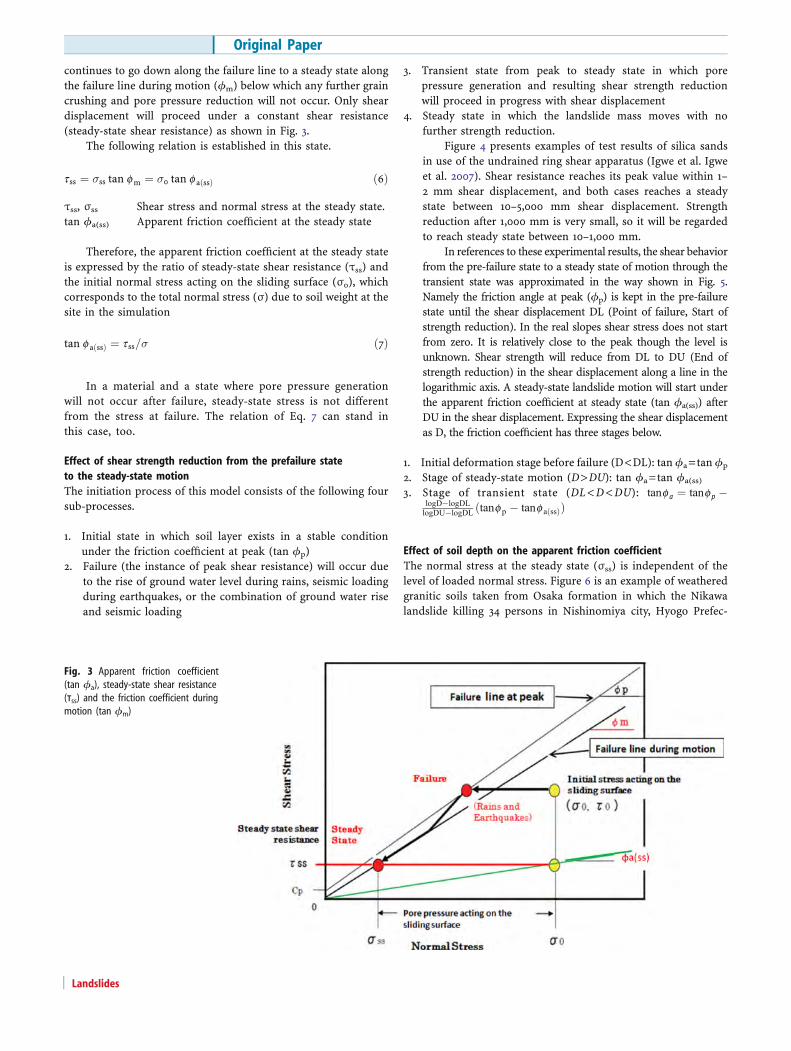
continues to go down along the failure line to a steady state alongthe failure line during motion (ϕm) below which any further graincrushing and pore pressure reduction will not occur. Only sheardisplacement will proceed under a constant shear resistance(steady-state shear resistance) as shown in Fig. 3.

The following relation is established in this state.

tss ¼ �ss tan fm ¼ �0 tan f aðssÞ ð6Þ

τss, σss Shear stress and normal stress at the steady state.tan ϕa(ss) Apparent friction coefficient at the steady state

Therefore, the apparent friction coefficient at the steady stateis expressed by the ratio of steady-state shear resistance (τss) andthe initial normal stress acting on the sliding surface (σ0), whichcorresponds to the total normal stress (σ) due to soil weight at thesite in the simulation

tan f aðssÞ ¼ tss=� ð7Þ

In a material and a state where pore pressure generationwill not occur after failure, steady-state stress is not differentfrom the stress at failure. The relation of Eq. 7 can stand inthis case, too.

Effect of shear strength reduction from the prefailure stateto the steady-state motionThe initiation process of this model consists of the following foursub-processes.

1. Initial state in which soil layer exists in a stable conditionunder the friction coefficient at peak (tan ϕp)

2. Failure (the instance of peak shear resistance) will occur dueto the rise of ground water level during rains, seismic loadingduring earthquakes, or the combination of ground water riseand seismic loading

3. Transient state from peak to steady state in which porepressure generation and resulting shear strength reductionwill proceed in progress with shear displacement

4. Steady state in which the landslide mass moves with nofurther strength reduction.

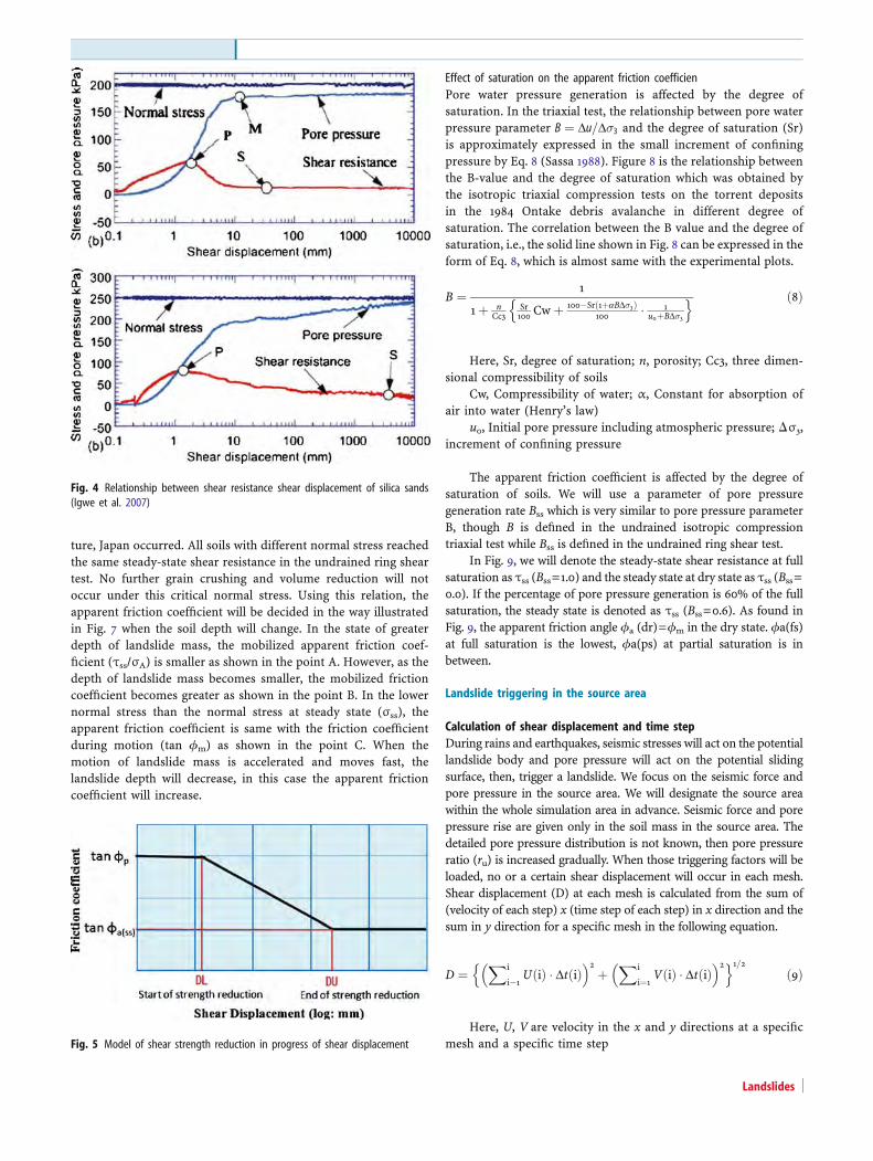
Figure 4 presents examples of test results of silica sandsin use of the undrained ring shear apparatus (Igwe et al. Igweet al. 2007). Shear resistance reaches its peak value within 1–2 mm shear displacement, and both cases reaches a steadystate between 10–5,000 mm shear displacement. Strengthreduction after 1,000 mm is very small, so it will be regardedto reach steady state between 10–1,000 mm.

In references to these experimental results, the shear behaviorfrom the pre-failure state to a steady state of motion through thetransient state was approximated in the way shown in Fig. 5.Namely the friction angle at peak (ϕp) is kept in the pre-failurestate until the shear displacement DL (Point of failure, Start ofstrength reduction). In the real slopes shear stress does not startfrom zero. It is relatively close to the peak though the level isunknown. Shear strength will reduce from DL to DU (End ofstrength reduction) in the shear displacement along a line in thelogarithmic axis. A steady-state landslide motion will start underthe apparent friction coefficient at steady state (tan ϕa(ss)) afterDU in the shear displacement. Expressing the shear displacementas D, the friction coefficient has three stages below.

1. Initial deformation stage before failure (D<DL): tan ϕa=tan ϕp

2. Stage of steady-state motion (D>DU): tan ϕa=tan ϕa(ss)

3. Stage of transient state (DL<D<DU): tanf a ¼ tanf p �logD�logDLlogDU�logDL ðtanf p � tanf aðssÞÞ

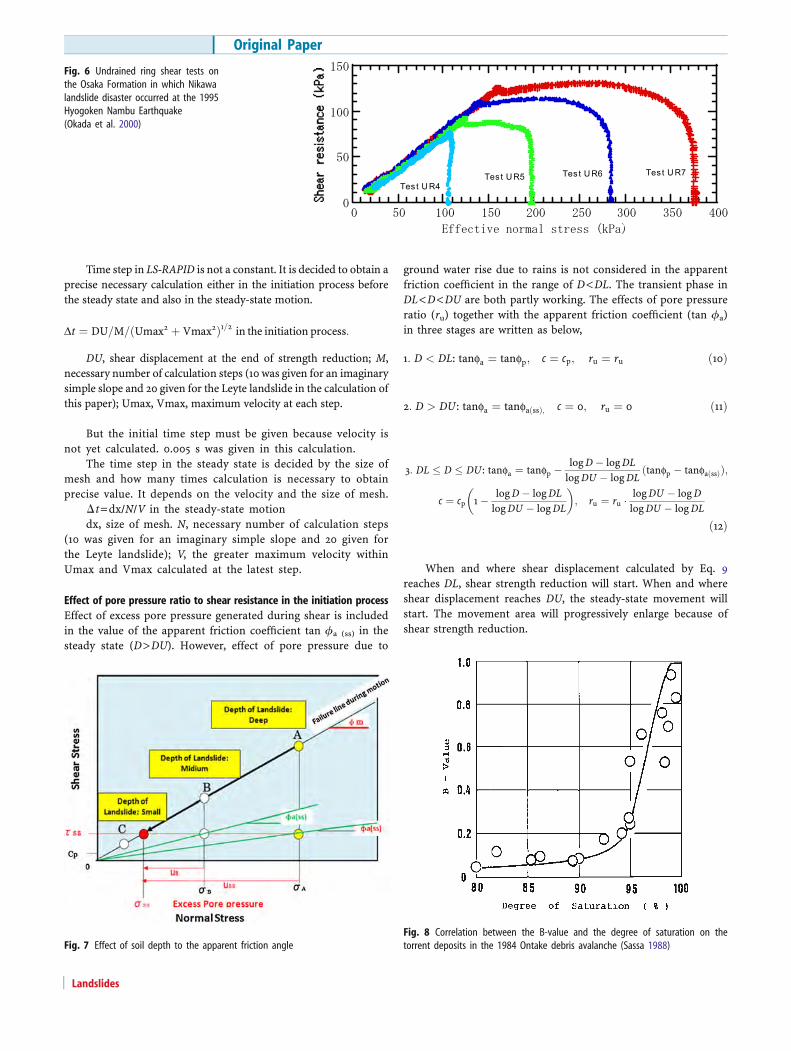
Effect of soil depth on the apparent friction coefficientThe normal stress at the steady state (σss) is independent of thelevel of loaded normal stress. Figure 6 is an example of weatheredgranitic soils taken from Osaka formation in which the Nikawalandslide killing 34 persons in Nishinomiya city, Hyogo Prefec-

Fig. 3 Apparent friction coefficient(tan ϕa), steady-state shear resistance(τss) and the friction coefficient duringmotion (tan ϕm)

Original Paper

Landslides

ture, Japan occurred. All soils with different normal stress reachedthe same steady-state shear resistance in the undrained ring sheartest. No further grain crushing and volume reduction will notoccur under this critical normal stress. Using this relation, theapparent friction coefficient will be decided in the way illustratedin Fig. 7 when the soil depth will change. In the state of greaterdepth of landslide mass, the mobilized apparent friction coef-ficient (τss/σA) is smaller as shown in the point A. However, as thedepth of landslide mass becomes smaller, the mobilized frictioncoefficient becomes greater as shown in the point B. In the lowernormal stress than the normal stress at steady state (σss), theapparent friction coefficient is same with the friction coefficientduring motion (tan ϕm) as shown in the point C. When themotion of landslide mass is accelerated and moves fast, thelandslide depth will decrease, in this case the apparent frictioncoefficient will increase.

Effect of saturation on the apparent friction coefficienPore water pressure generation is affected by the degree ofsaturation. In the triaxial test, the relationship between pore waterpressure parameter B ¼ Du=D�3 and the degree of saturation (Sr)is approximately expressed in the small increment of confiningpressure by Eq. 8 (Sassa 1988). Figure 8 is the relationship betweenthe B-value and the degree of saturation which was obtained bythe isotropic triaxial compression tests on the torrent depositsin the 1984 Ontake debris avalanche in different degree ofsaturation. The correlation between the B value and the degree ofsaturation, i.e., the solid line shown in Fig. 8 can be expressed in theform of Eq. 8, which is almost same with the experimental plots.

B ¼ 1

1þ nCc3

Sr100 Cw þ 100�Srð1þaBD�3Þ

100 � 1u0þBD�3

n o ð8Þ

Here, Sr, degree of saturation; n, porosity; Cc3, three dimen-sional compressibility of soils

Cw, Compressibility of water; α, Constant for absorption ofair into water (Henry’s law)

u0, Initial pore pressure including atmospheric pressure; Δσ3,increment of confining pressure

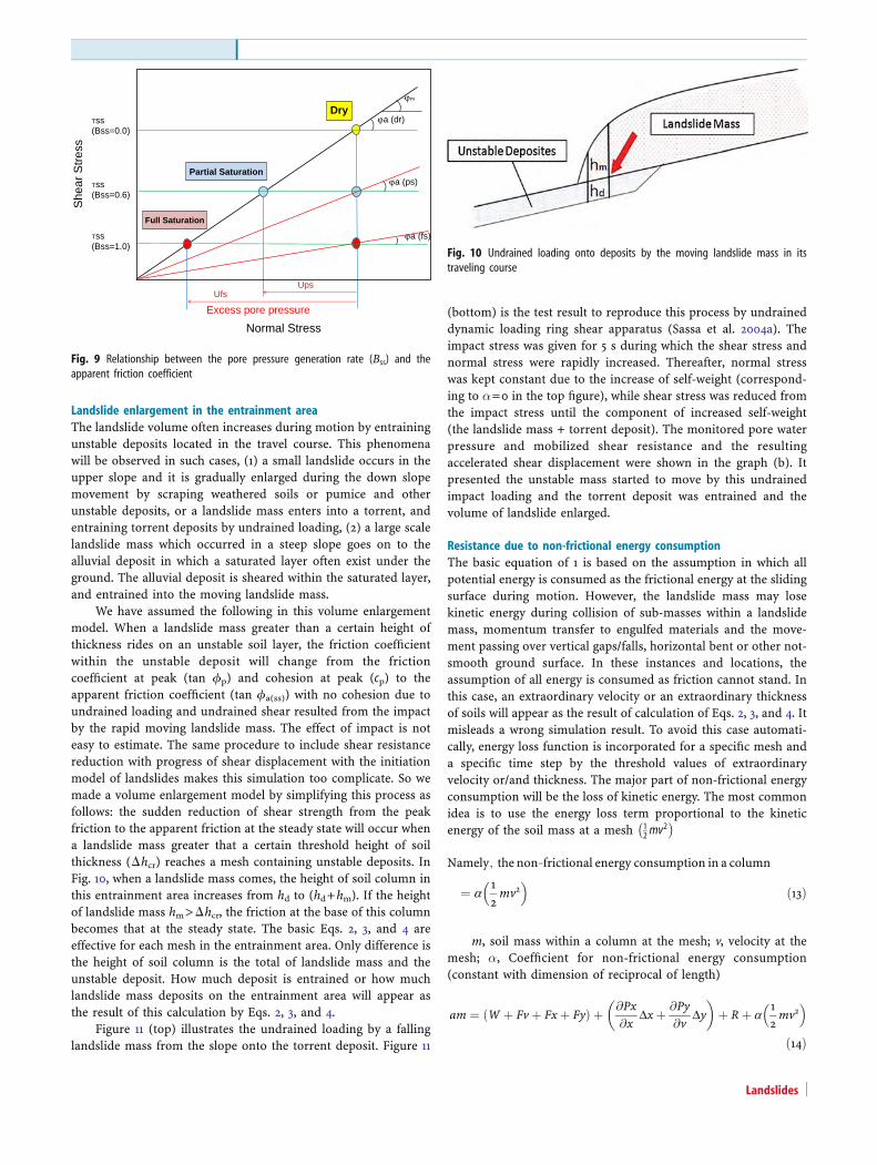
The apparent friction coefficient is affected by the degree ofsaturation of soils. We will use a parameter of pore pressuregeneration rate Bss which is very similar to pore pressure parameterB, though B is defined in the undrained isotropic compressiontriaxial test while Bss is defined in the undrained ring shear test.

In Fig. 9, we will denote the steady-state shear resistance at fullsaturation as τss (Bss=1.0) and the steady state at dry state as τss (Bss=0.0). If the percentage of pore pressure generation is 60% of the fullsaturation, the steady state is denoted as τss (Bss=0.6). As found inFig. 9, the apparent friction angle ϕa (dr)=ϕm in the dry state. ϕa(fs)at full saturation is the lowest, ϕa(ps) at partial saturation is inbetween.

Landslide triggering in the source area

Calculation of shear displacement and time stepDuring rains and earthquakes, seismic stresses will act on the potentiallandslide body and pore pressure will act on the potential slidingsurface, then, trigger a landslide. We focus on the seismic force andpore pressure in the source area. We will designate the source areawithin the whole simulation area in advance. Seismic force and porepressure rise are given only in the soil mass in the source area. Thedetailed pore pressure distribution is not known, then pore pressureratio (ru) is increased gradually. When those triggering factors will beloaded, no or a certain shear displacement will occur in each mesh.Shear displacement (D) at each mesh is calculated from the sum of(velocity of each step) x (time step of each step) in x direction and thesum in y direction for a specific mesh in the following equation.

D ¼Xi

i�1UðiÞ � DtðiÞ

� �2þ

Xi

i¼1VðiÞ � DtðiÞ

� �2n o1=2ð9Þ

Here, U, V are velocity in the x and y directions at a specificmesh and a specific time step

Fig. 4 Relationship between shear resistance shear displacement of silica sands(Igwe et al. 2007)

Fig. 5 Model of shear strength reduction in progress of shear displacement

Landslides

Time step in LS-RAPID is not a constant. It is decided to obtain aprecise necessary calculation either in the initiation process beforethe steady state and also in the steady-state motion.

Dt ¼ DU=M=ðUmax2 þ Vmax2Þ1=2 in the initiation process:

DU, shear displacement at the end of strength reduction; M,necessary number of calculation steps (10 was given for an imaginarysimple slope and 20 given for the Leyte landslide in the calculation ofthis paper); Umax, Vmax, maximum velocity at each step.

But the initial time step must be given because velocity isnot yet calculated. 0.005 s was given in this calculation.

The time step in the steady state is decided by the size ofmesh and how many times calculation is necessary to obtainprecise value. It depends on the velocity and the size of mesh.

Δt=dx/N/V in the steady-state motiondx, size of mesh. N, necessary number of calculation steps

(10 was given for an imaginary simple slope and 20 given forthe Leyte landslide); V, the greater maximum velocity withinUmax and Vmax calculated at the latest step.

Effect of pore pressure ratio to shear resistance in the initiation processEffect of excess pore pressure generated during shear is includedin the value of the apparent friction coefficient tan ϕa (ss) in thesteady state (D>DU). However, effect of pore pressure due to

ground water rise due to rains is not considered in the apparentfriction coefficient in the range of D<DL. The transient phase inDL<D<DU are both partly working. The effects of pore pressureratio (ru) together with the apparent friction coefficient (tan ϕa)in three stages are written as below,

1: D < DL: tanfa ¼ tanfp; c ¼ cp; ru ¼ ru ð10Þ

2: D > DU : tanfa ¼ tanfaðssÞ; c ¼ 0; ru ¼ 0 ð11Þ

3: DL � D � DU : tanfa ¼ tanfp �logD� logDLlogDU � logDL

ðtanfp � tanfaðssÞÞ;

c ¼ cp 1� logD� logDLlogDU � logDL

� �; ru ¼ ru � logDU � logD

logDU � logDL

ð12Þ

When and where shear displacement calculated by Eq. 9reaches DL, shear strength reduction will start. When and whereshear displacement reaches DU, the steady-state movement willstart. The movement area will progressively enlarge because ofshear strength reduction.

Fig. 6 Undrained ring shear tests onthe Osaka Formation in which Nikawalandslide disaster occurred at the 1995Hyogoken Nambu Earthquake(Okada et al. 2000)

Fig. 7 Effect of soil depth to the apparent friction angleFig. 8 Correlation between the B-value and the degree of saturation on thetorrent deposits in the 1984 Ontake debris avalanche (Sassa 1988)

Original Paper

Landslides

Landslide enlargement in the entrainment areaThe landslide volume often increases during motion by entrainingunstable deposits located in the travel course. This phenomenawill be observed in such cases, (1) a small landslide occurs in theupper slope and it is gradually enlarged during the down slopemovement by scraping weathered soils or pumice and otherunstable deposits, or a landslide mass enters into a torrent, andentraining torrent deposits by undrained loading, (2) a large scalelandslide mass which occurred in a steep slope goes on to thealluvial deposit in which a saturated layer often exist under theground. The alluvial deposit is sheared within the saturated layer,and entrained into the moving landslide mass.

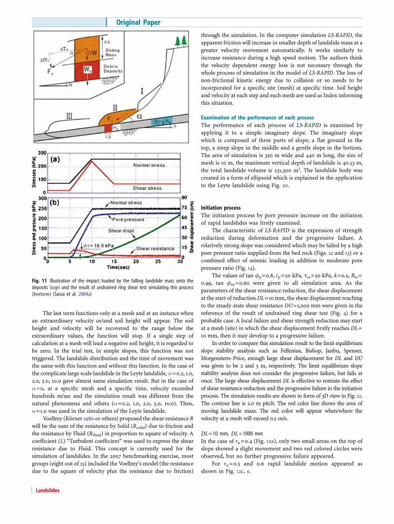
We have assumed the following in this volume enlargementmodel. When a landslide mass greater than a certain height ofthickness rides on an unstable soil layer, the friction coefficientwithin the unstable deposit will change from the frictioncoefficient at peak (tan ϕp) and cohesion at peak (cp) to theapparent friction coefficient (tan ϕa(ss)) with no cohesion due toundrained loading and undrained shear resulted from the impactby the rapid moving landslide mass. The effect of impact is noteasy to estimate. The same procedure to include shear resistancereduction with progress of shear displacement with the initiationmodel of landslides makes this simulation too complicate. So wemade a volume enlargement model by simplifying this process asfollows: the sudden reduction of shear strength from the peakfriction to the apparent friction at the steady state will occur whena landslide mass greater that a certain threshold height of soilthickness (Δhcr) reaches a mesh containing unstable deposits. InFig. 10, when a landslide mass comes, the height of soil column inthis entrainment area increases from hd to (hd+hm). If the heightof landslide mass hm>Δhcr, the friction at the base of this columnbecomes that at the steady state. The basic Eqs. 2, 3, and 4 areeffective for each mesh in the entrainment area. Only difference isthe height of soil column is the total of landslide mass and theunstable deposit. How much deposit is entrained or how muchlandslide mass deposits on the entrainment area will appear asthe result of this calculation by Eqs. 2, 3, and 4.

Figure 11 (top) illustrates the undrained loading by a fallinglandslide mass from the slope onto the torrent deposit. Figure 11

(bottom) is the test result to reproduce this process by undraineddynamic loading ring shear apparatus (Sassa et al. 2004a). Theimpact stress was given for 5 s during which the shear stress andnormal stress were rapidly increased. Thereafter, normal stresswas kept constant due to the increase of self-weight (correspond-ing to α=0 in the top figure), while shear stress was reduced fromthe impact stress until the component of increased self-weight(the landslide mass + torrent deposit). The monitored pore waterpressure and mobilized shear resistance and the resultingaccelerated shear displacement were shown in the graph (b). Itpresented the unstable mass started to move by this undrainedimpact loading and the torrent deposit was entrained and thevolume of landslide enlarged.

Resistance due to non-frictional energy consumptionThe basic equation of 1 is based on the assumption in which allpotential energy is consumed as the frictional energy at the slidingsurface during motion. However, the landslide mass may losekinetic energy during collision of sub-masses within a landslidemass, momentum transfer to engulfed materials and the move-ment passing over vertical gaps/falls, horizontal bent or other not-smooth ground surface. In these instances and locations, theassumption of all energy is consumed as friction cannot stand. Inthis case, an extraordinary velocity or an extraordinary thicknessof soils will appear as the result of calculation of Eqs. 2, 3, and 4. Itmisleads a wrong simulation result. To avoid this case automati-cally, energy loss function is incorporated for a specific mesh anda specific time step by the threshold values of extraordinaryvelocity or/and thickness. The major part of non-frictional energyconsumption will be the loss of kinetic energy. The most commonidea is to use the energy loss term proportional to the kineticenergy of the soil mass at a mesh 1

2mv2

�

Namely; the non�frictional energy consumption in a column

¼ a12mv2

� �ð13Þ

m, soil mass within a column at the mesh; v, velocity at themesh; α, Coefficient for non-frictional energy consumption(constant with dimension of reciprocal of length)

am ¼ ðW þ Fvþ Fxþ FyÞ þ @Px@x

Dxþ @Py@v

Dy� �

þ Rþ a12mv2

� �

ð14Þ

Partial Saturation

ϕa (dr)

ϕa (ps)

ϕa (fs)

ϕm

Excess pore pressure

UpsUfs

Normal Stress

Dry

Full Saturation

Tss(Bss=0.0)

She

ar S

tres

s

Tss (Bss=0.6)

Tss (Bss=1.0)

Fig. 9 Relationship between the pore pressure generation rate (Bss) and theapparent friction coefficient

Fig. 10 Undrained loading onto deposits by the moving landslide mass in itstraveling course

Landslides

The last term functions only at a mesh and at an instance whenan extraordinary velocity or/and soil height will appear. The soilheight and velocity will be recovered to the range below theextraordinary values, the function will stop. If a single step ofcalculation at a mesh will lead a negative soil height, it is regarded tobe zero. In the trial test, in simple slopes, this function was nottriggered. The landslide distribution and the time of movement wasthe same with this function and without this function. In the case ofthe complicate large scale landslide in the Leyte landslide, α=0.2, 1.0,2.0, 5.0, 10.0 gave almost same simulation result. But in the case ofα=0, at a specific mesh and a specific time, velocity exceededhundreds m/sec and the simulation result was different from thenatural phenomena and others (α=0.2, 1.0, 2.0, 5.0, 10.0). Then,α=1.0 was used in the simulation of the Leyte landslide.

Voellmy (Körner 1980 or others) proposed the shear resistanceRwill be the sum of the resistance by Solid (Rsolid) due to friction andthe resistance by Fluid (Rfluid) in proportion to square of velocity. Acoefficient (ξ) “Turbulent coefficient” was used to express the shearresistance due to Fluid. This concept is currently used for thesimulation of landslides. In the 2007 benchmarking exercise, mostgroups (eight out of 13) included the Voellmy’s model (the resistancedue to the square of velocity plus the resistance due to friction)

through the simulation. In the computer simulation LS-RAPID, theapparent friction will increase in smaller depth of landslide mass at agreater velocity movement automatically. It works similarly toincrease resistance during a high speed motion. The authors thinkthe velocity dependent energy loss is not necessary through thewhole process of simulation in the model of LS-RAPID. The loss ofnon-frictional kinetic energy due to collision or so needs to beincorporated for a specific site (mesh) at specific time. Soil heightand velocity at each step and each mesh are used as Index informingthis situation.

Examination of the performance of each processThe performance of each process of LS-RAPID is examined byapplying it to a simple imaginary slope. The imaginary slopewhich is composed of three parts of slope; a flat ground in thetop, a steep slope in the middle and a gentle slope in the bottom.The area of simulation is 350 m wide and 440 m long, the size ofmesh is 10 m, the maximum vertical depth of landslide is 40.53 m,the total landslide volume is 231,300 m3. The landslide body wascreated in a form of ellipsoid which is explained in the applicationto the Leyte landslide using Fig. 20.

Initiation processThe initiation process by pore pressure increase on the initiationof rapid landslides was firstly examined.

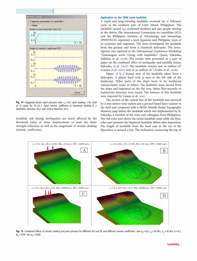
The characteristic of LS-RAPID is the expression of strengthreduction during deformation and the progressive failure. Arelatively strong slope was considered which may be failed by a highpore pressure ratio supplied from the bed rock (Figs. 12 and 13) or acombined effect of seismic loading in addition to moderate porepressure ratio (Fig. 14).

The values of tan ϕp=0.8, cp=50 kPa, τss=50 kPa, k=0.5, Bss=0.99, tan ϕm=0.60 were given to all simulation area. As theparameters of the shear resistance reduction, the shear displacementat the start of reductionDL=10mm, the shear displacement reachingto the steady-state shear resistance DU=1,000 mm were given in thereference of the result of undrained ring shear test (Fig. 4) for aprobable case. A local failure and shear strength reduction may startat a mesh (site) in which the shear displacement firstly reaches DL=10 mm, then it may develop to a progressive failure.

In order to compare this simulation result to the limit equilibriumslope stability analysis such as Fellenius, Bishop, Janbu, Spenser,Morgenstern–Price, enough large shear displacement for DL and DUwas given to be 2 and 5 m, respectively. The limit equilibrium slopestability analysis does not consider the progressive failure, but fails atonce. The large shear displacement DL is effective to restrain the effectof shear resistance reduction and the progressive failure in the initiationprocess. The simulation results are shown in form of 3D view in Fig. 12.The contour line is 2.0 m pitch. The red color line shows the area ofmoving landslide mass. The red color will appear when/where thevelocity at a mesh will exceed 0.5 m/s.

DL=10 mm, DL=1000 mmIn the case of ru=0.4 (Fig. 12a), only two small areas on the top ofslope showed a slight movement and two red colored circles wereobserved, but no further progressive failure appeared.

For ru=0.5 and 0.6 rapid landslide motion appeared asshown in Fig. 12c, e.

Fig. 11 Illustration of the impact loaded by the falling landslide mass onto thedeposits (top) and the result of undrained ring shear test simulating this process(bottom) (Sassa et al. 2004a)

Original Paper

Landslides

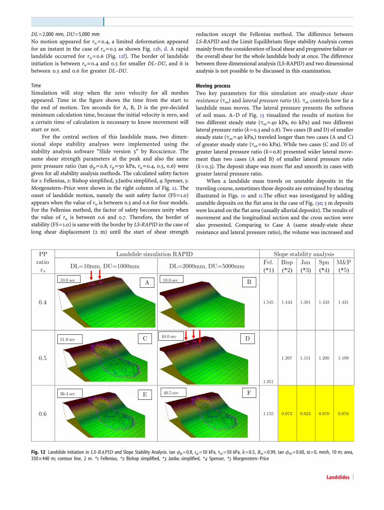
DL=2,000 mm, DU=5,000 mmNo motion appeared for ru=0.4, a limited deformation appearedfor an instant in the case of ru=0.5 as shown Fig. 12b, d. A rapidlandslide occurred for ru=0.6 (Fig. 12f). The border of landslideinitiation is between ru=0.4 and 0.5 for smaller DL–DU, and it isbetween 0.5 and 0.6 for greater DL–DU.

TimeSimulation will stop when the zero velocity for all meshesappeared. Time in the figure shows the time from the start tothe end of motion. Ten seconds for A, B, D is the pre-decidedminimum calculation time, because the initial velocity is zero, anda certain time of calculation is necessary to know movement willstart or not.

For the central section of this landslide mass, two dimen-sional slope stability analyses were implemented using thestability analysis software “Slide version 5” by Rocscience. Thesame shear strength parameters at the peak and also the samepore pressure ratio (tan ϕp=0.8, cp=50 kPa, ru=0.4, 0.5, 0.6) weregiven for all stability analysis methods. The calculated safety factorsfor 1: Fellenius, 2: Bishop simplified, 3:Janbu simplified, 4: Spenser, 5:Morgenstern–Price were shown in the right column of Fig. 12. Theonset of landslide motion, namely the unit safety factor (FS=1.0)appears when the value of ru is between 0.5 and 0.6 for four models.For the Fellenius method, the factor of safety becomes unity whenthe value of ru is between 0.6 and 0.7. Therefore, the border ofstability (FS=1.0) is same with the border by LS-RAPID in the case oflong shear displacement (2 m) until the start of shear strength

reduction except the Fellenius method. The difference betweenLS-RAPID and the Limit Equilibrium Slope stability Analysis comesmainly from the consideration of local shear and progressive failure orthe overall shear for the whole landslide body at once. The differencebetween three dimensional analysis (LS-RAPID) and two dimensionalanalysis is not possible to be discussed in this examination.

Moving processTwo key parameters for this simulation are steady-state shearresistance (τss) and lateral pressure ratio (k). τss controls how far alandslide mass moves. The lateral pressure presents the softnessof soil mass. A–D of Fig. 13 visualized the results of motion fortwo different steady state (τss=40 kPa, 60 kPa) and two differentlateral pressure ratio (k=0.3 and 0.8). Two cases (B and D) of smallersteady state (τss=40 kPa,) traveled longer than two cases (A and C)of greater steady state (τss=60 kPa). While two cases (C and D) ofgreater lateral pressure ratio (k=0.8) presented wider lateral move-ment than two cases (A and B) of smaller lateral pressure ratio(k=0.3). The deposit shape was more flat and smooth in cases withgreater lateral pressure ratio.

When a landslide mass travels on unstable deposits in thetraveling course, sometimes those deposits are entrained by shearingillustrated in Figs. 10 and 11.The effect was investigated by addingunstable deposits on the flat area in the case of Fig. 13e; 5 m depositswere located on the flat area (usually alluvial deposits). The results ofmovement and the longitudinal section and the cross section werealso presented. Comparing to Case A (same steady-state shearresistance and lateral pressure ratio), the volume was increased and

Fig. 12 Landslide initiation in LS-RAPID and Slope Stability Analysis. tan ϕp=0.8, cp=50 kPa, τss=50 kPa, k=0.5, Bss=0.99, tan ϕm=0.60, α=0, mesh, 10 m; area,350×440 m; contour line, 2 m. *1 Fellenius, *2 Bishop simplified, *3 Janbu simplified, *4 Spenser, *5 Morgenstern–Price

Landslides

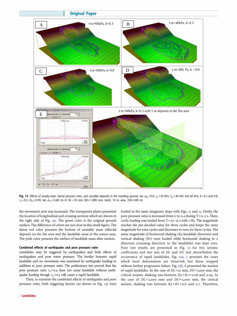
the movement area was increased. The transparent plates presentedthe location of longitudinal and crossing sections which are shown inthe right side of Fig. 13e. The green color is the original groundsurface. The difference of colors are not clear in this small figure. Thedense red color presents the bottom of unstable mass (alluvialdeposit) on the flat area and the landslide mass in the source area.The pink color presents the surface of landslide mass after motion.

Combined effects of earthquake and pore pressure ratioLandslides may be triggered by earthquakes and both effects ofearthquakes and pore water pressure. The border between rapidlandslide and no movement was examined by earthquake loading inaddition to pore pressure ratio. The preliminary test proved that thepore pressure ratio ru=0.4 does not cause landslide without earth-quake loading though ru=0.5 will cause a rapid landslide.

Then, to examine the combined effects of earthquake and porepressure ratio, both triggering factors (as shown in Fig. 14) were

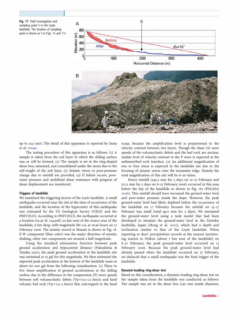
loaded in the same imaginary slope with Figs. 12 and 13. Firstly, thepore pressure ratio is increased from 0 to 0.4 during T=0–5 s. Then,cyclic loading was loaded from T=10–25 s with 1 Hz. The magnitudereaches the pre-decided value for three cycles and keeps the samemagnitude for nine cycles and decreases to zero for three cycles. Thesame magnitude of horizontal shaking (Ky-landslide direction) andvertical shaking (Kv) were loaded while horizontal shaking in xdirection (crossing direction to the landslide) was kept zero.Four test results are presented in Fig. 15 for two seismiccoefficients and two sets of DL and DU just above/below theoccurrence of rapid landslides. Fig. 15a, c presents the caseswhich local deformation are observed, but those stoppedwithout further progressive failure. Fig. 15b, d presented the motionof rapid landslides. In the case of DL=10 mm, DU=1,000 mm, thecritical seismic shaking was between Ky=Kv=0.08 and 0.09. Inthe case of DL=2,000 mm and DU=5,000 mm, the criticalseismic shaking was between Ky=Kv=0.6 and 0.7. Therefore,

τ ss=60kPa, k=0.8 τ ss=40k Pa, k =0.8

τ ss=60kPa, k=0.3 τ ss=40kPa, k=0.3

τ ss=60kPa, k=0.3 with 5 m deposits in the flat area

A B

C D

E

Fig. 13 Effects of steady-state, lateral pressure ratio, and unstable deposits in the traveling ground. tan ϕp=0.8; cp=50 kPa; τss=40 kPa and 60 kPa; k=0.3 and 0.8;ru=0.5; Bss=0.99; tan ϕm=0.60; α=0; DL=10 mm; DU=1,000 mm; mesh, 10 m; area, 350×440 m)

Original Paper

Landslides

landslide risk during earthquakes are much affected by thethreshold value of shear displacement to start the shearstrength reduction as well as the magnitude of seismic shaking(seismic coefficient).

Application to the 2006 Leyte landslideA rapid and long-traveling landslide occurred on 17 February2006 in the southern part of Leyte Island, Philippines. Thelandslide caused 154 confirmed fatalities and 990 people missingin the debris. The International Consortium on Landslides (ICL)and the Philippine Institute of Volcanology and Seismology(PHIVOLCS) organized a joint Japanese and Philippine team of22 scientists and engineers. The team investigated the landslidefrom the ground and from a chartered helicopter. The inves-tigation was reported at the International Conference-Workshop“Guinsaugon 2008—Living with landslides” (Sassa, Fukuoka,Solidum et al. 2008). The results were presented as a part ofpaper on the combined effect of earthquake and rainfalls (Sassa,Fukuoka, et al. 2007). The landslide volume was 20 million m3

(Catane et al. 2007) and 16–30 million m3 (Araiba et al. 2008).Figure 16 is a frontal view of the landslide taken from a

helicopter. A planer hard rock is seen at the left side of theheadscarp. Other parts of the slope seem to be weatheredvolcanoclastic rocks or debris. The landslide mass moved fromthe slope and deposited on the flat area. Many flow-mounds orhummocky structure were found. The features of this landslidewere reported by Catane et al. 2007.

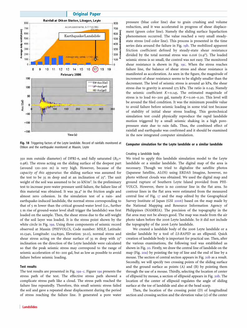
The section of the central line of the landslide was surveyedby a non-mirror total station and a ground-based laser scanner inthe field and compared with a SRTM (Shuttle Radar TopographyMission) map before the landslide which was implemented by H.Fukuoka, a member of the team and colleagues from Philippines.The red-color part shows the initial landslide mass while the blue-color part presents the displaced landslide debris after deposition.The length of landslide from the head scar to the toe of thedeposition is around 4 km. The inclination connecting the top of

Fig. 14 Triggering factors (pore pressure ratio: ru=0.4, cyclic loading: 1 Hz, totalof 15 cycles for 10–25 s, Same seismic coefficient in horizontal shaking in y(landslide) direction (Ky) and vertical direction (Kv)

Fig. 15 Combined effects of seismic loading and pore pressure for different DU and DL and different seismic coefficients. (tan fp=0.8, cp=50 kPa, τss=50 kPa, k=0.5,Bss=0.99, tan fm=0.60)

Landslides

the initial landslide and the toe of the displaced landslide depositis approximately 10°, which indicates the average apparent frictionangle mobilized during the whole travel distance. The value ismuch smaller than the usual friction angle of debris (sandygravel) of 30–40°. Therefore, it suggests that high excess pore-waterpressure was generated during motion. Figure 17b shows a flowmound that traveled from the initial slope to this flat area withoutmuch disturbance. Movement without much disturbance is possiblewhen the shear resistance on the sliding surface became very low; thus,movement of the material is like that of a sled.

The material of the flow mound is volcanoclastic debris,including sand and gravel. We observed the material in the sourcearea by eye observation from the surface and by hand scoopexcavation in the valley-side slope after the landslide. It consisted ofvolcanoclastic debris or strongly weathered volcanoclastic rocks. It isregarded to be the same material (either disturbed or intact)observed in the flow mound shown in Fig. 17. Therefore, we took asample of about 100 kg from the base of the flow mound shown inthe point “S” in the section of Fig. 17a) and the photo of Fig. 17b. The

location is in the center of travel course and just below the sourcearea. Then, we transported the material to Japan and subjected it tothe undrained dynamic-loading ring-shear test.

Testing apparatusThe undrained dynamic-loading ring-shear apparatus (DPRI-3)was developed from 1992 to 2004 (DPRI-7). The basic concept ofthis apparatus is to reproduce the formation of sliding surfaceand its post-failure motion by reproducing the stress acting onthe sliding zone and to observe the generated pore water pressure,mobilized shear resistance and post-failure rapid motion. It canprovide seismic stress in addition to gravity and pore-waterpressure as triggering factors. The leakage of pore water from theedge of rotating half and stable half is prevented by a rubber edgewhich is pressed at a contact pressure greater than the pore waterpressure inside the shear box by servo-control system. Theapparatus used for this test is DPRI-6, which is capable to dotests under dynamic loading, up to 5 Hz, and high-speed shearing,

S

Manila

LandslidLandslide

Philippines

Fig. 16 The front view of the Leytelandslide on 17 February 2006.(Taken by K. Sassa from a charteredhelicopter. S sampling point)

Original Paper

Landslides

up to 224 cm/s. The detail of this apparatus is reported by Sassaet al. 2004a.

The testing procedure of this apparatus is as follows: (1) Asample is taken from the soil layer in which the sliding surfacewas or will be formed, (2) The sample is set in the ring-shapedshear box, saturated, and consolidated under the stress due to theself-weight of the soil layer, (3) Seismic stress or pore-pressurechange due to rainfall are provided, (4) If failure occurs, pore-water pressure and mobilized shear resistance with progress ofshear displacement are monitored.

Triggers of landslideWe examined the triggering factors of the Leyte landslide. A smallearthquake occurred near the site at the time of occurrence of thelandslide, and the location of the hypocenter of this earthquakewas estimated by the US Geological Survey (USGS) and thePHIVOLCS. According to PHIVOLCS, the earthquake occurred ata location (10.30 N, 124.90E) 22 km west of the source area of thelandslide, 6 km deep, with magnitude Ms 2.6, at 10:36 hours on 17February 2006. The seismic record at Maasin is shown in Fig. 18.E-W component (blue color) was the major direction of seismicshaking, other two components are around a half magnitude.

Using the standard attenuation function between peakground acceleration and hypocentral distance (Fukushima &Tanaka 1990), the peak ground acceleration at the landslide sitewas estimated at 10 gal for this magnitude. We then estimated theexpected peak acceleration at the bottom of the landslide mass asabout 60–200 gal from the following consideration. (1) Three tofive times amplification of ground accelerations at the slidingsurface due to the difference in the compression (P) wave speedsbetween soft volcanoclastic debris (Vp=0.5–1.5 km/s) and hardvolcanic bed rock (Vp=2.5–5 km/s) that outcropped in the head

scarp, because the amplification level is proportional to thevelocity contrast between two layers. Though the shear (S) wavespeeds of the volcanoclastic debris and the bed rock are unclear,similar level of velocity contrast to the P wave is expected at thesediment/bed rock interface. (2) An additional magnification oftwo to four times is expected in the landslide site due to thefocusing of seismic waves onto the mountain ridge. Namely thetotal magnification of this site will be 6–20 times.

Heavy rainfall (459.2 mm for 3 days on 10–12 February and571.2 mm for 5 days on 8–12 February 2006) occurred in this areabefore the day of the landslide as shown in Fig. 18a (PAGASA2006). This rainfall should have increased the ground-water leveland pore-water pressure inside the slope. However, the peakground-water level had likely depleted before the occurrence ofthe landslide on 17 February because the rainfall on 13–17February was small (total 99.0 mm for 5 days). We simulatedthe ground-water level using a tank model that had beendeveloped to simulate the ground-water level in the Zentokulandslide, Japan (Hong et al. 2005), which had a depth andinclination similar to that of the Leyte landslide. Wheninputting 10 days’ precipitation records at the nearest monitor-ing station in Otikon (about 7 km west of the landslide) on8–17 February, the peak ground-water level occurred on 13February 2006. Because the peak ground-water level hadalready passed when the landslide occurred on 17 February,we deduced that a small earthquake was the final trigger of thelandslide.

Dynamic-loading ring-shear testBased on this consideration, a dynamic-loading ring-shear test onthe sample taken from the landslide was conducted as follows:The sample was set in the shear box (250 mm inside diameter,

A

B

SFig. 17 Field investigation andsampling point S in the Leytelandslide. The location of samplingpoint is shown as S in Figs. 16 and 17a

Landslides

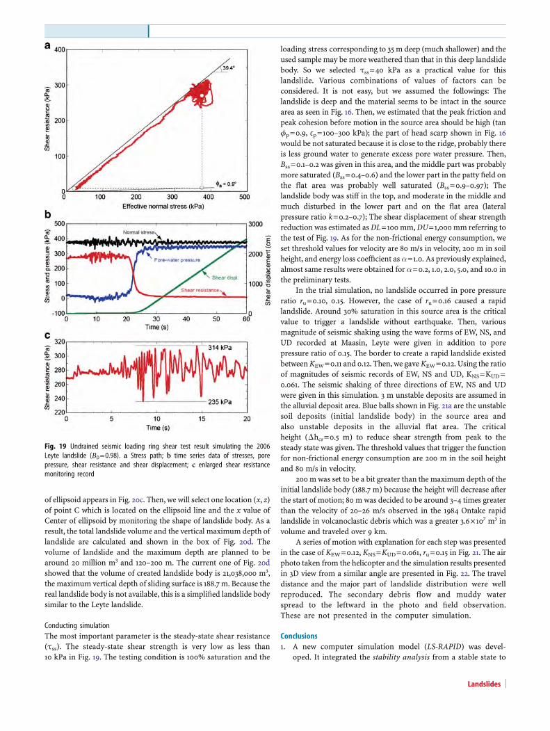
350 mm outside diameter) of DPRI-6, and fully saturated (BD=0.98). The stress acting on the sliding surface of the deepest part(around 120–200 m) is very high. However, because of thecapacity of this apparatus: the sliding surface was assumed forthe test to be 35 m deep and at an inclination of 25°. The unitweight of the soil was assumed to be 20 kN/m3. In the preliminarytest to increase pore-water pressure until failure, the failure line ofthis material was obtained. It was 39.4° in the friction angle andalmost zero cohesion. In the simulation test of a rain- andearthquake-induced landslide, the normal stress corresponding tothat of 5 m lower than the critical ground-water level (i.e., further5 m rise of ground-water level shall trigger the landslide) was firstloaded on the sample. Then, the shear stress due to the self-weightof the soil layer was loaded. It is the stress point shown by thewhite circle in Fig. 19a. Using three components of seismic recordobserved at Massin (PHIVOLCS, Code number: MSLP, Latitude:10.1340, Longitude: 124.8590, Elevation: 50.0), normal stress andshear stress acting on the shear surface of 35 m deep with 25°inclination on the direction of the Leyte landslide were calculatedso that the peak seismic stress may correspond to the range ofseismic acceleration of 60–200 gal, but as low as possible to avoidfailure before seismic loading.

Test resultsThe test results are presented in Fig. 19a–c. Figure 19a presents thestress path of the test. The effective stress path showed acomplicate stress path like a cloud. The stress path reached thefailure line repeatedly. Therefore, this small seismic stress failedthe soil and gave a repeated shear displacement during the periodof stress reaching the failure line. It generated a pore water

pressure (blue color line) due to grain crushing and volumereduction, and it was accelerated in progress of shear displace-ment (green color line). Namely the sliding surface liquefactionphenomenon occurred. The value reached a very small steady-state stress (red color line). This process is presented in the timeseries data around the failure in Fig. 19b. The mobilized apparentfriction coefficient defined by steady-state shear resistancedivided by the total normal stress was 0.016 (0.9°). The loadedseismic stress is so small, the control was not easy. The monitoredshear resistance is shown in Fig. 19c. When the stress reachesfailure line, the balance of shear stress and shear resistance ismanifested as acceleration. As seen in the figure, the magnitude ofincrement of shear resistance seems to be slightly smaller than thedecrement. The level of seismic stress is around 40 kPa, the shearstress due to gravity is around 275 kPa. The ratio is 0.145. Namelythe seismic coefficient K=0.145. The estimated magnitude ofstress is to load 60–200 gal, namely K=0.06–0.20. This level willbe around the filed condition. It was the minimum possible valueto avoid failure before seismic loading in some trial test becauseof stability of initial shear stress loading. This geotechnicalsimulation test could physically reproduce the rapid landslidemotion triggered by a small seismic shaking in a high pore-pressure state due to rain falls. Thus, the combined effect ofrainfall and earthquake was confirmed and it should be examinedin the new integrated computer simulation.

Computer simulation for the Leyte landslide or a similar landslide

Creating a landslide bodyWe tried to apply this landslide simulation model to the Leytelandslide or a similar landslide. The digital map of the area isnecessary. Though we tried to digitalize the satellite photos(Japanese Satellite, ALOS) using ERDAS Imagine, however, nophoto without clouds was obtained. We used the digital map andground rupture of Southern Leyte Island provided from PHI-VOLCS. However, there is no contour line in the flat area. Socontour lines in the flat area were estimated from the measuredcentral line of Fig. 17 and the map edited by the GeographicalSurvey Institute of Japan (GSI 2006) based on the map made bythe National Mapping and Resource Information Agency ofPhilippines (NAMRIA). The precision of the topography in theflat area may not be always good. The map was made from the airphoto taken before the 2006 Leyte landslide. So it did not includethe topography of the 2006 Leyte landslide.

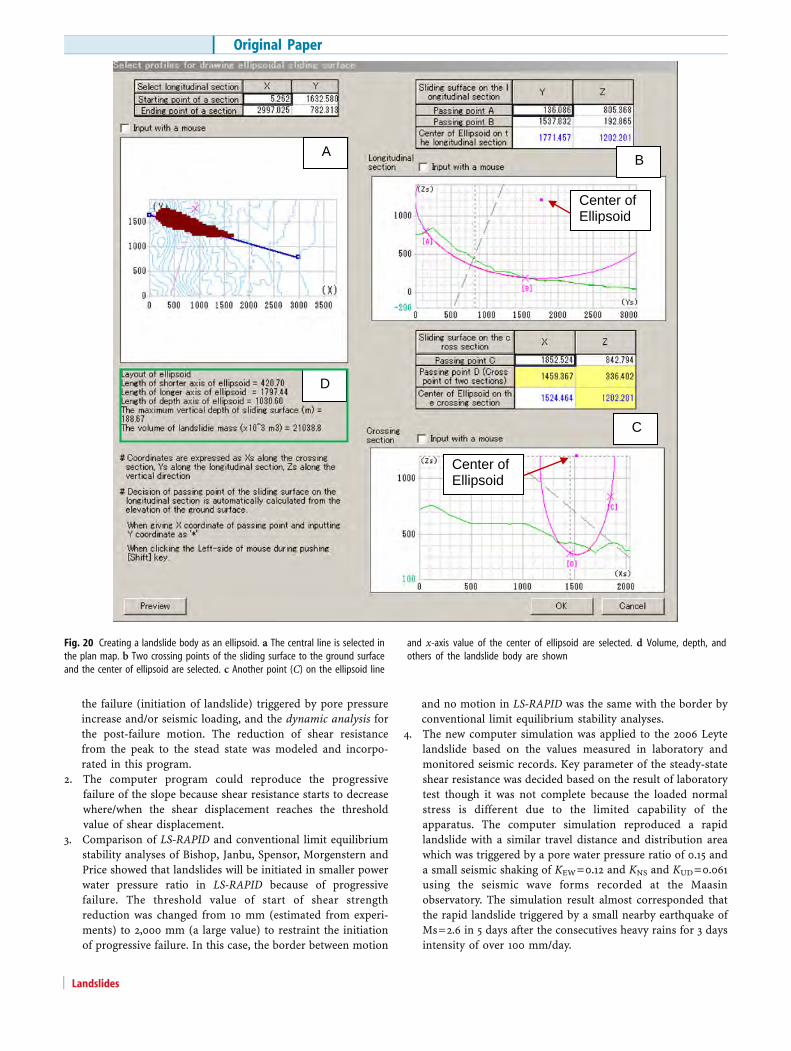
We created a landslide body of the 2006 Leyte landslide or asimilar landslide by a tool of LS-RAPID as an ellipsoid. Quickcreation of landslide body is important for practical use. Then, afterthe various examinations, the following tool was established asshown in Fig. 20. Firstly, we draw the central line of landslide on themap (Fig. 20a) by pointing the top of line and the end of line by amouse. The section of central section appears in Fig. 20b as a result.Secondly, we will specify two crossing points of the sliding surfaceand the ground surface as points (A) and (B) by pointing themthrough the use of a mouse. Thirdly, selecting the location of centerof ellipsoid by mouse, a section of ellipsoid appears in Fig. 20b. Thelocation of the center of ellipsoid regulates the angle of slidingsurface at the toe of landslide and also at the head scarp.

Then, the location of the crossing point (D) of longitudinalsection and crossing section and the elevation value (z) of the center

Fig. 18 Triggering factors of the Leyte landslide. Record of rainfalls monitored atOtikon and the earthquake monitored at Maasin, Leyte

Original Paper

Landslides

of ellipsoid appears in Fig. 20c. Then, we will select one location (x, z)of point C which is located on the ellipsoid line and the x value ofCenter of ellipsoid by monitoring the shape of landslide body. As aresult, the total landslide volume and the vertical maximum depth oflandslide are calculated and shown in the box of Fig. 20d. Thevolume of landslide and the maximum depth are planned to bearound 20 million m3 and 120–200 m. The current one of Fig. 20dshowed that the volume of created landslide body is 21,038,000 m3,the maximum vertical depth of sliding surface is 188.7m. Because thereal landslide body is not available, this is a simplified landslide bodysimilar to the Leyte landslide.

Conducting simulationThe most important parameter is the steady-state shear resistance(τss). The steady-state shear strength is very low as less than10 kPa in Fig. 19. The testing condition is 100% saturation and the

loading stress corresponding to 35m deep (much shallower) and theused sample may be more weathered than that in this deep landslidebody. So we selected τss=40 kPa as a practical value for thislandslide. Various combinations of values of factors can beconsidered. It is not easy, but we assumed the followings: Thelandslide is deep and the material seems to be intact in the sourcearea as seen in Fig. 16. Then, we estimated that the peak friction andpeak cohesion before motion in the source area should be high (tanϕp=0.9, cp=100–300 kPa); the part of head scarp shown in Fig. 16would be not saturated because it is close to the ridge, probably thereis less ground water to generate excess pore water pressure. Then,Bss=0.1–0.2 was given in this area, and the middle part was probablymore saturated (Bss=0.4–0.6) and the lower part in the patty field onthe flat area was probably well saturated (Bss=0.9–0.97); Thelandslide body was stiff in the top, and moderate in the middle andmuch disturbed in the lower part and on the flat area (lateralpressure ratio k=0.2–0.7); The shear displacement of shear strengthreduction was estimated asDL=100mm,DU=1,000mm referring tothe test of Fig. 19. As for the non-frictional energy consumption, weset threshold values for velocity are 80 m/s in velocity, 200 m in soilheight, and energy loss coefficient as α=1.0. As previously explained,almost same results were obtained for α=0.2, 1.0, 2.0, 5.0, and 10.0 inthe preliminary tests.

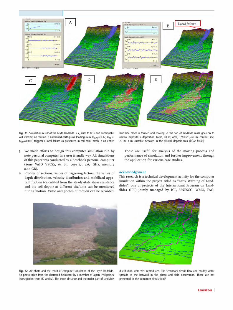
In the trial simulation, no landslide occurred in pore pressureratio ru=0.10, 0.15. However, the case of ru=0.16 caused a rapidlandslide. Around 30% saturation in this source area is the criticalvalue to trigger a landslide without earthquake. Then, variousmagnitude of seismic shaking using the wave forms of EW, NS, andUD recorded at Maasin, Leyte were given in addition to porepressure ratio of 0.15. The border to create a rapid landslide existedbetweenKEW=0.11 and 0.12. Then, we gaveKEW=0.12. Using the ratioof magnitudes of seismic records of EW, NS and UD, KNS=KUD=0.061. The seismic shaking of three directions of EW, NS and UDwere given in this simulation. 3 m unstable deposits are assumed inthe alluvial deposit area. Blue balls shown in Fig. 21a are the unstablesoil deposits (initial landslide body) in the source area andalso unstable deposits in the alluvial flat area. The criticalheight (Δhcr=0.5 m) to reduce shear strength from peak to thesteady state was given. The threshold values that trigger the functionfor non-frictional energy consumption are 200 m in the soil heightand 80 m/s in velocity.

200mwas set to be a bit greater than the maximum depth of theinitial landslide body (188.7 m) because the height will decrease afterthe start of motion; 80 m was decided to be around 3–4 times greaterthan the velocity of 20–26 m/s observed in the 1984 Ontake rapidlandslide in volcanoclastic debris which was a greater 3.6×107 m3 involume and traveled over 9 km.

A series of motion with explanation for each step was presentedin the case of KEW=0.12, KNS=KUD=0.061, ru=0.15 in Fig. 21. The airphoto taken from the helicopter and the simulation results presentedin 3D view from a similar angle are presented in Fig. 22. The traveldistance and the major part of landslide distribution were wellreproduced. The secondary debris flow and muddy waterspread to the leftward in the photo and field observation.These are not presented in the computer simulation.

Conclusions1. A new computer simulation model (LS-RAPID) was devel-

oped. It integrated the stability analysis from a stable state to

Fig. 19 Undrained seismic loading ring shear test result simulating the 2006Leyte landslide (BD=0.98). a Stress path; b time series data of stresses, porepressure, shear resistance and shear displacement; c enlarged shear resistancemonitoring record

Landslides

the failure (initiation of landslide) triggered by pore pressureincrease and/or seismic loading, and the dynamic analysis forthe post-failure motion. The reduction of shear resistancefrom the peak to the stead state was modeled and incorpo-rated in this program.

2. The computer program could reproduce the progressivefailure of the slope because shear resistance starts to decreasewhere/when the shear displacement reaches the thresholdvalue of shear displacement.

3. Comparison of LS-RAPID and conventional limit equilibriumstability analyses of Bishop, Janbu, Spensor, Morgenstern andPrice showed that landslides will be initiated in smaller powerwater pressure ratio in LS-RAPID because of progressivefailure. The threshold value of start of shear strengthreduction was changed from 10 mm (estimated from experi-ments) to 2,000 mm (a large value) to restraint the initiationof progressive failure. In this case, the border between motion

and no motion in LS-RAPID was the same with the border byconventional limit equilibrium stability analyses.

4. The new computer simulation was applied to the 2006 Leytelandslide based on the values measured in laboratory andmonitored seismic records. Key parameter of the steady-stateshear resistance was decided based on the result of laboratorytest though it was not complete because the loaded normalstress is different due to the limited capability of theapparatus. The computer simulation reproduced a rapidlandslide with a similar travel distance and distribution areawhich was triggered by a pore water pressure ratio of 0.15 anda small seismic shaking of KEW=0.12 and KNS and KUD=0.061using the seismic wave forms recorded at the Maasinobservatory. The simulation result almost corresponded thatthe rapid landslide triggered by a small nearby earthquake ofMs=2.6 in 5 days after the consecutives heavy rains for 3 daysintensity of over 100 mm/day.

D

A B

C

Center of Ellipsoid

Center of Ellipsoid

Fig. 20 Creating a landslide body as an ellipsoid. a The central line is selected inthe plan map. b Two crossing points of the sliding surface to the ground surfaceand the center of ellipsoid are selected. c Another point (C) on the ellipsoid line

and x-axis value of the center of ellipsoid are selected. d Volume, depth, andothers of the landslide body are shown

Original Paper

Landslides

5. We made efforts to design this computer simulation run bynote personal computer in a user friendly way. All simulationsof this paper was conducted by a notebook personal computer(Sony VAIO VPCZ1, 64 bit, core i7, 2.67 GHz, memory8.00 GB).

6. Profiles of sections, values of triggering factors, the values ofdepth distribution, velocity distribution and mobilized appa-rent friction (calculated from the steady-state shear resistanceand the soil depth) at different site/time can be monitoredduring motion. Video and photos of motion can be recorded.

Those are useful for analysis of the moving process andperformance of simulation and further improvement throughthe application for various case studies.

AcknowledgementThis research is a technical development activity for the computersimulation within the project titled as “Early Warning of Land-slides”, one of projects of the International Program on Land-slides (IPL) jointly managed by ICL, UNESCO, WMO, FAO,

A

C D E

B

Fig. 21 Simulation result of the Leyte landslide. a ru rises to 0.15 and earthquakewill start but no motion. b Continued earthquake loading (Max K(EW)=0.12, KNS=KUD=0.061) triggers a local failure as presented in red color mesh, c an entire

landslide block is formed and moving, d the top of landslide mass goes on toalluvial deposits, e deposition. Mesh, 40 m; Area, 1,960×3,760 m; contour line,20 m; 3 m unstable deposits in the alluvial deposit area (blue balls)

Fig. 22 Air photo and the result of computer simulation of the Leyte landslide.Air photo taken from the chartered helicopter by a member of Japan–Philippinesinvestigation team (K. Araiba). The travel distance and the major part of landslide

distribution were well reproduced. The secondary debris flow and muddy waterspreads to the leftward in the photo and field observation. Those are notpresented in the computer simulation@

Landslides

UNISDR, ICSU and WFEO. The project was financially supportedby the Ministry of Education, Culture, Sports, Science andTechnology of Japan (MEXT) in the frame work of InternationalJoint Research Promotion Fund. The project (leader: K. Sassa) wasjointly conducted by the International Consortium on Landslides(ICL) and the Disaster Prevention Research Institute (DPRI) ofKyoto University, the China Geological Survey, the Korean Instituteof Geosience and Mineral Resources (KIGAM) and the NationalInstitute for Disaster Prevention (NIDP) in Korea, University ofGadjah Mada (UGM) and the Bandung Institute of Technology(ITB) of Indonesia, Philippine Institute of Volcanology andSeismology (PHIVOLCS). The part of Leyte landslide investigationwas conducted together with Assoc. Prof. Hiroshi Fukuoka, Prof.Hideaki Marui, Assoc Prof. Fawu Wang and Dr Wang Gonghui.

References

Araiba K, Nagura H, Jeong B, Koarai M, Sato H, Osanai N, Itoh H, Sassa K (2008)Topography of failed and deposited areas of the large collapse in Southern Leyte,Philippines occurred on 17 February 2006. In: Proc. International Conference onManagement of Landslide Hazard in the Asia-Pacific Region (Satellite Symposium onthe First World Landslide Forum). pp 434–443

Catane SG, Cabria HB, Tomarong CP, Saturay RM, Zarco MA, Pioquinto WC (2007)Catastrophic rockslide-debris avalanche at St. Bernard, Southern Leyte, Philippines.Landslides 4(1):85–90

Chen H, Lee CF (2003) A dynamic mode for rainfall-induced landslides on naturalslopes. Geomorphology 51:269–288

Chen H, Lee CF (2007) Landslide mobility analysis using MADFLOW. Proc The 2007International Forum on Landslide Disaster Management 2:857–874

Denlinger RP, Iverson RM (2004) Granular avalanches across irregular three-dimensionalterrain: 1. Theory and computation. J Geophys Res 106(F01014):14

Fukushima Y, Tanaka T (1990) A new attenuation relation for peak horizontal accelerationof strong earthquake ground motion in Japan. Bull Seismol Soc Am 84:757–783

GSI (2006) 1:50,000 topographical map “Surroundding area of Leyte landslide”,Geological Survey Institute of Japan

Hong Y, Hiura H, Shino K, Sassa K, Fukuoka H (2005) Quantitative assessment on theinfluence of heavy rainfall on the crystalline schist aldnslide by monitoirng system—case study on Zentoku landslide in Japan. Landslides 2-1:31–41

Hungr O (2009) Numerical modelling of the motion of rapid, flow-like landslides forhazard assessment. KSCE J Civ Eng 13(4):281–287

Hungr O, KcKinnon M, McDougall S.(2007a). Two models for analysis of landslidemotion: Application to the 2007 Hong Kong benchmarking exersies. In: Proc. the2007 International Forum on landslide disaster management, vol. 2. pp 919–932

Hungr O, Morgenstern NR, Wong HN (2007b). Review of benchmarking exercise onlandslide debris runout and mobility modelling. In: Proc. the 2007 InternationalForum on landslide disaster management, vol. 2. pp 755–812

Igwe O, Sassa K, Wang FW (2007) The influence of grading on the shear strength ofloose sands in stress-controlled ring shear tests. Landslides 4(1):43–51

Körner, H (1980). Model conceptions for the rock slide and avalanche movement. Proc.Iternational Symposium ”INTERPRAEVENT 1980”, Bad Ischl, vol. 2. pp 15–55

Kwan J, Sun HW (2007). Benchmarking exersise on landslide mobility modelling-runoutanayses using 3dDMM. In: Proc. the 2007 International Forum on landslide disastermanagement, vol.2. pp 945–966

Okada Y, Sassa K, Fukuoka H (2000) Liquefaction and the steady state of weatheredgranite sands obtained by undrained ring shear tests: a fundamental study on themechanism of liquidized landslides. J Nat Disaster Sci 22(2):75–85

Philippine Atmospheric, Geophysical and Astronomical Services Agency (PAGASA) (2006)Precipitation record at Otikon, Libagon

PHIVOLCS (2008) Digital map and ground rupture of Southern Leyte Island. PhilippineInstitute of Volcanology and Seismology (PHIVOLCS) in CD

Sassa K (1988) Geotechnical model for the motion of landslides. In: Proc. 5th InternationalSymposium on Landslides, “Landslides”, Balkema, Rotterdam, vol. 1. pp 37–56

Sassa K, Fukuoka H, Wang G, Ishikawa N (2004a) Undrained dynamic-loading ring-shearapparatus and its application to landslide dynamics. Landslides 1(1):7–19

Sassa K, Wang G, Fukuoka H, Wang FW, Ochiai T, Sugiyama, Sekiguchi T (2004b)Landslide risk evaluation and hazard mapping for rapid and long-travel landslides inurban development areas. Landslides 1(3):221–235

Sassa K, Fukuoka H, Wang FW, Wang GH (2007) Landslides induced by a combinedeffects of earthquake and rainfall. Progress in Landslide Science (Editors: Sassa ,Fukuoka, Wang, Wang), Springer, Berlin. pp 311–325

Sassa K, Fukuoka H, Solidum R, Wang G, Marui H, Furumura T, Wang F (2008) Mechanism ofthe initiation and motion of the 2006 Leyte landslide, Philippines. In: Proc InternationalConference-Workshop “Guinsaugon 2008—Living with Landslides (in CD)

Stone R (2009) Peril in the Pamirs. Science 326:1614–1617Takahashi T, Tsujimoto H (2000) A mechanical model for Merapi-type pyroclastic flow. J

Volcanol Geotherm Res 98:91–115Wang FW, Sassa K (2007). Landslide simulation by geotechnical model adopting a

model for variable apparent friction coefficient. In: Proc. the 2007 InternationalForum on landslide disaster management, vol. 2. pp 1079–1096

Zhang D, Sassa K (1996) A study of the apparent friction angle after failure duringundrained shear of loess soils. J Japan Soc Erosion Control Eng 49(3):20–27

K. Sassa ()) : O. NagaiInternational Consortium on Landslides,Kyoto, Japane-mail: sassa@iclhq.orge-mail: nagai@iclhq.org

R. SolidumPhilippine Institute of Volcanology and Seismology (PHIVOLCS),Quezon City, Philippinese-mail: solidr@phivolcs.dost.gov.ph

Y. YamazakiGODAI Development Corporation,Kanazawa, Japane-mail: yamazaki@godai.co.jp

H. OhtaOhta Geo-Research Co., Ltd.,Nishinomiya, Japane-mail: ohta@ohta-geo.co.jp

Original Paper

Landslides