Kollisjonsanalyse mellom flytende vindturbin og ...

Mathias Tomren Viktor Aanesen

Kollisjonsanalyse mellom flytende

vindturbin og installasjonsfartøy

Bacheloroppgave i Marinteknikk

Bergen, Norge 2020

Kollisjonsanalyse mellom flytende vindturbin og

installasjonsfartøy

Mathias Tomren

Viktor Aanesen

Institutt for Maskin- og Marinfag

Høgskulen på Vestlandet

NO-5063 Bergen, Norge

IMM 2020-M33

Høgskulen på Vestlandet Fakultet for Ingeniør- og Naturvitskap Institutt for maskin- og marinfag Inndalsveien 28 NO-5063 Bergen, Norge Omslag fotografi © Norbert Lümmen

English title: Collision analysis between a floating wind turbine and an installation vessel

Forfatter(e), studentnummer: Mathias Tomren, 180307

Viktor Aanesen, 571635 Studieprogram: Marinteknikk Dato: 05 2020 Rapportnummer: IMM 2020-M33 Veileder ved HVL: David Roger Lande-Sudall, Førsteamanuensis IMM, HVL Thore Clifford Thuestad, Førstelektor IMM, HVL Oppdragsgiver: Equinor Oppdragsgivers referanse: Gudmund Per Olsen

Antall filer levert digitalt: 2

Kollisjonsanalyse mellom flytende vindturbin og installasjonsfartøy

5

Forord

Denne bacheloroppgaven er gjennomført ved institutt for maskin- og marinfag, IMM ved

Høgskolen på Vestlandet, HVL. Oppgaven er gjennomført i tidsrommet januar 2020 til mai

2020. Oppgaven er skrevet av kandidatene Mathias Tomren og Viktor Aanesen, i

kollaborasjon med gruppe M32, Daniel W. Ekerhovd og Stian N. Boge. Oppgaven er

gjennomført i samarbeid med Equinor. Interne veiledere for bacheloroppgaven er David

Roger Lande-Sudall, førsteamanuensis ved IMM, og Thore Clifford Thuestad, førstelektor

ved IMM. Gruppen kom i kontakt med Equinor høsten 2020 via HVLs bachelor oppgaver.

Etter samtaler med Equinor og interne veiledere ble endelig utforming av oppgaven bestemt.

Oppgaven går ut på å teste om et fartøy med halvt nedsenkbare egenskaper vil redusere

kollisjonskreftene med vindturbinen ved installasjon. Resultatene fra oppgaven presenteres på

artikkelform.

Takk til

Kandidatene ønsker å rette en stor takk til de som har hjulpet oss å gjennomføre oppgaven:

David Roger Lande-Sudall og Thore Clifford Thuestad, interne veiledere ved HVL, for

veiledning under gjennomføring av oppgaven.

Idunn Olimb og Bernt Karsten Lyngvær, eksterne veileder ved Equinor, for godt

samarbeid og informative samtaler.

Mathias Tomren Viktor Aanesen

Mathias Tomren, Viktor Aanesen

6


7

Sammendrag

Flytende vindturbiner som benytter sparbøyfundamenter har vist seg å være en effektiv

løsning for å utnytte havvind som ren energi. En negativ faktor for sparbøyfundamentet er at

det behøver en stor dypgang for å beholde stabilitet. Antallet mulige havner for installasjon er

derfor redusert til et fåtall. Tidligere arbeid har forsket på om det er mulig å redusere

dypgangen på vindturbinen ved å benytte en lekter som et installasjonsfartøy. Ved

eksperimentell testing av kobling mellom lekter og vindturbin har det oppstått kollisjoner ved

avkobling av uønsket størrelse. Derfor vil det i denne oppgaven fokuseres på å se om et fartøy

med halvt nedsenkbare egenskaper kan redusere disse kollisjonskreftene med vindturbinen

ved numeriske analyser.

De numeriske analysene er gjennomført for fire installasjonsfartøyer; en numerisk versjon av

lekteren som ble benyttet eksperimentelt, og tre halvt nedsenkbare fartøyer med noe

forskjellige geometrier. Analysene for fartøyene er gjennomført for to scenarioer, der det

første har forankret installasjonsfartøyene og vindturbinen, og det andre er kun

installasjonsfartøyene forankret. Begge scenarioene er gjennomført med bølgeretning 0° og

180°, og bølgehøyder H = 1.5 m og H = 2.9 m. Resultatene fra analysene viste at de halvt

nedsenkbare fartøyene har en reduksjon av gjennomsnittlig kollisjonsimpuls mellom 35-66%

avhengig av parameterne, som bølgeretning, bølgehøyde og bølgeperiode.


8


9

Abstract

Floating wind turbines (FWTs) utilizing spar-buoy platforms have proven to be a rigid

solution to harness clean energy from offshore wind. A downside to the spar-buoy concept is

the great draught needed to maintain stability, which in turn reduces the number of possible

quayside assembly and installation locations. Previous work investigating a possible draught

reduction of the floating wind turbine using a barge type installation vessel is here continued

with the use of a numerical method. During the experimental testing, large collision impulses

between the barge and the FWT were registered for higher wave heights. Therefore, the

numerical analysis focuses on collision impulses between the installation vessel and FWT.

The numerical analysis is run for four installation vessels: a numerical version of the

experimental barge, and three vessels with semi-submersible properties, with some

geometrical differences. Analysis are performed with moored installation vessel, and with

moored and unmoored FWT. Wave directions for 0° and 180°, with wave height, H = 1.5 m,

and H = 2.9 m, are performed for all vessels. Both wave directions are examined in the

numerical work with results showing a reduction in mean collision impulse between 35-66%

when using a vessel with semi-submersible properties, depending on test parameters, such as

wave period, wave height and wave direction.


10


11

Innholdsfortegnelse Forord ..................................................................................................................................................................... 5

Sammendrag ........................................................................................................................................................... 7

Abstract ................................................................................................................................................................... 9

1. Innledning ......................................................................................................................................................... 13

1.1 Bakgrunn og motivasjon .............................................................................................................................. 13

1.2 Mål for oppgaven ......................................................................................................................................... 14

1.3 Synopsis ....................................................................................................................................................... 15

2. Teori .................................................................................................................................................................. 16

2.1 De seks frihetsgrader ................................................................................................................................... 16

2.2 Regulære lineære bølger .............................................................................................................................. 16

2.3. RAO ............................................................................................................................................................ 18

2.4 Egenperiode og egenfrekvens ...................................................................................................................... 18

2.5 Massematrise ............................................................................................................................................... 19

2.6 Impuls .......................................................................................................................................................... 20

3. Programvare ..................................................................................................................................................... 20

3.1 SESAM ........................................................................................................................................................ 20

3.2 MATLAB .................................................................................................................................................... 22

4. Metode ............................................................................................................................................................... 23

4.1 Utvikling av konsept .................................................................................................................................... 23

4.2 Modellering.................................................................................................................................................. 23

4.2.1 Halvt nedsenkbare fartøy ..................................................................................................................... 24

4.2.2 Lekter ................................................................................................................................................... 26

4.2.3 Flytende vindturbin .............................................................................................................................. 28

4.3 Hydrodynamisk beregning ........................................................................................................................... 30

4.4 Numeriskkollisjonsanalyse .......................................................................................................................... 33

5. Introduksjon til artikkel ................................................................................................................................. 35

6. Oppsummering og konklusjon ........................................................................................................................ 36

6.1 Oppsummering av funn ............................................................................................................................... 36

TT1 – Forankret fartøy og turbin .................................................................................................................. 36

TT2 – Forankret fartøy .................................................................................................................................. 37

6.2 Konklusjon ................................................................................................................................................... 37

7. Fremtidig arbeid .............................................................................................................................................. 38

8. Feilkilder ........................................................................................................................................................... 39

9. Referanser ......................................................................................................................................................... 40

Vedlegg .................................................................................................................................................................. 41


12


13

1. Innledning

1.1. Bakgrunn og motivasjon

Det er for tiden stort fokus på den globale overgangen til lavkarbonsamfunnet, samt bruk av

fornybare energikilder for å tilfredsstille verdens økende behov for elektrisk energi. I følge

Equinor kommer havvind til å spille en nøkkelrolle i denne prosessen [1].

Vind til havs har potensialet til å generere i overkant av 420 000 TWh per år verden

over, dette tilsvarer mer enn 18 ganger verdens elektriske energibehov i dag [2]. Nær 80% av

dette potensialet ligger i havområder med havdyp større enn 60 meter hvor vinden er sterkere

og mer konsis [1]. Når havdypet øker, vil flytende vindturbiner være eneste alternativ for å

kunne utnytte denne energien da bunnfaste vindturbiner normalt har en begrensning på 50

meter. En flytende vindturbin er en vindturbin som er montert oppå en flytende konstruksjon

og holdes på plass ved hjelp av forankring til havbunnen. Det vil i denne oppgaven fokuseres

på Equinor sin Hywind løsning og da spesielt utformingen benyttet i pilot prosjektet deres

Hywind Scotland som var verdens første flytende havvindpark. Hywind konseptet benytter

sparbøye som den flytende konstruksjon som vindturbinen er montert oppå. En sparbøye er en

dyp vertikal flytende fundament, med lavt vannlinjeareal og har god stabilitet grunnet et

tyngdepunkt som er plassert under oppdriftssenteret. Sammenstillingen av vindturbinene for

Hywind Scotland foregikk i en dyp fjord utenfor Stord i Vestland fylke ved hjelp av verdens

største flytende kranfartøy, Saipem 7000 [3]. Montering av vindturbinene nært land kan gi en

fordel ved at det antageligvis er en rimeligere prosess sammenlignet med den som gjøres med

de bunnfaste turbinene som monteres og installeres offshore. En av de store utfordringene ved

dette konseptet er sparbøyens store dypgang, som på vindturbinen installert i Hywind

Scotland er over 70 meter. Dette gir store begrensninger med tanke på lokasjoner for

montering, da det finnes få lokasjoner i verden med havner som har dette dypet. Også ruten ut

til lokasjon fra havnen må være dyp nok til at vindturbinene kan slepes ut. En annen faktor

som gir begrensninger til denne installasjons metoden er bruken av flytende kranfartøy. Når et

stort antall flytende vindturbiner skal installeres verden over vil det være behov for å lage nye

fartøyer spesifikk til jobben. Dette er kostbart dersom det skal gjennomføres få installasjoner,

men lønner seg dersom det blir mange installasjoner. For at sparbøye konseptet skal bli mer

tilgjengelig og benyttes flere steder i verden arbeides det med ulike metoder for å gjøre denne

installasjonen på. I 2014 avholdt Equinor en innovasjonskonkurranse hvor flere installasjons

konsepter ble presentert. Fra de innsendte forslagene ble det kåret tre konsepter som vinnere;

MODEC, Ulstein og Atkins [4].


14

MODEC og Ulstein sine konsepter baserer seg på et fartøy som transporterer ferdig monterte

turbiner og tårn ut til lokasjon som monteres på spar-fundamentet som er slept ut og forankret

på forhånd. Metodene skilles fra hverandre ved en noe ulik sammenkoblings metode mellom

turbintårn og spar-fundament. Atkins sitt forslag er en gjenbrukbar transportramme for opptil

fire turbiner, metoden reduserer spar-fundamentets dypgang og gir en økt stabilitet når de fire

turbinene er koblet til rammen ved at de fungerer som et halvt nedsenkbare fartøy. Den

reduserte dypgangen gir også mulighet til installasjon nært kai, som fjerner behovet for løft

ved bruk av flytende kranfartøy [5].

Fra før har Atkins sin metode vært inspirasjon for en masteroppgave [6] og en påfølgende

konferanseartikkel [7] hvor fokuset har vært å kartlegge veltende moment som oppstår i

koblingen mellom fartøyet og de flytende vindturbinene, samt mulige kollisjoner mellom de

to. I disse prosjektene ble det utført modellforsøk hvor transportrammen til Atkins ble byttet

ut med en lekter, og kun en flytende vindturbinene med forenklet geometri tilkoblet forut på

lekteren for å forenkle modellforsøket. Begge prosjektene ga gode resultater som viste at både

moment og kollisjoner mellom fartøy og vindturbinen kunne håndteres ved hjelp av relativt

enkle tiltak, men det var fortsatt noen usikkerheter som gjør at det er verdt å jobbe videre

med. Med disse prosjektene som bakgrunn vil denne oppgaven fokusere videre på

egenskapene til selve installasjons fartøyet, og hva de betyr for de ulike kreftene som oppstår

mellom fartøyet og den flytende vindturbinen.

1.2. Mål for oppgaven

Målet for oppgaven er å undersøke om et installasjonsfartøy med egenskaper likt et halvt-

nedsenkbart fartøy vil kunne resultere i en reduksjon av kollisjonskrefter mellom

installasjonsfartøyet og den flytende vindturbinen når den skal slippes løs fra fartøyet.

For å undersøke dette vil det genereres tre numeriske modeller med egenskaper som er

typiske for et halvt-nedsenkbart fartøy. De tre modellene har alle samme hoveddimensjoner

og utforming, men har ulik dimensjonering på søylene mellom pongtong og dekk for å kunne

undersøke effekten som vannlinjearealet til fartøyet har. Figur (1) illustrerer lekteren og de tre

ulike modellene av det nye installasjonsfartøyet, og deres ulikheter.


15

Det skal i tillegg genereres en numerisk modell av lekteren som ble benyttet i de to tidligere

prosjektene, samt en numerisk modell av den flytende vindturbinen benyttet i Hywind

Scotland. Det er ønskelig å utføre analyser av oppsettet som ble benyttet i de tidligere

prosjektene for å avdekke om den numeriske metoden gir lignende resultater som den

eksperimentelle, samt for å kunne sammenligne den nye utformingen på fartøyet med

lekteren. Den numeriske modellen av vindturbinen vil bli benyttet i alle kollisjonsanalysene

uavhengig av fartøystype. Resultatene fra analysene vil bli behandlet i MATLAB for å

illustrere og kalkulerer de ulike parameterne som skal beregnes. Ved hjelp av dette vil

resultatene fra analysene fremstilles på en god og oversiktlig måte.

Figur (1): Illustrasjon av fartøyer benyttet i kollisjonsanalysen. Fra venstre NV-1, NV-2, NV-3, lekter.

1.3. Synopsis

I seksjon 2 og 3 presenteres teori og programvare som er benyttet for å gjennomføre de

numeriske analysene. Videre i seksjon 4 presenteres utviklingen av konseptene og

modelleringen av de fem benyttede elementene. I seksjon 5 presenteres den fullstendige

artikkelen med beskrivelse av gjennomføring, resultater og konklusjon. Avslutningsvis tar

seksjon 6 for seg en oppsummering av resultatene presentert i seksjon 5 samt konklusjon,

videre arbeid og feilkilder er presentert i seksjon 7 og 8.


16

2. Teori

Denne seksjonen foretar en gjennomgang av relevant teori benyttet i oppgaven. Teoridelen

introduseres med bevegelsessystem og dynamikk for flytende konstruksjoner, og avsluttes

med forklaring om beregning av massematrise og impulskrefter.

2.1. De seks frihetsgrader

Et flytende legeme har seks uavhengige bevegelser og kan beskrives som et system med seks

frihetsgrader, ofte referert til som 6 DOF. Dette betyr at legemet kan bevege seg i tre

retninger, også kjent som translasjoner, og rotere i tre retninger som vist i Figur (2). De seks

bevegelsene er definert som bevegelse av legemets tyngdepunkt og rotasjon om et sett av

vinkelrette akser gjennom tyngdepunktet. De tre translasjonene kalles for jag (surge), svai

(sway) og hiv (heave), som er henholdsvis bevegelse langs x, y og z-akse. De tre

rotasjonsbevegelsene kalles rull (roll), stamp (pitch) og gir (yaw), som er henholdsvis rotasjon

om x, y og z-akse [8].

Figur (2): De seks frihetsgrader for et flytende legeme [8].

2.2. Regulære lineære bølger

Den enkleste bølgeteorien anskaffes ved at bølgehøyden antas å være mindre enn både

bølgelengden og vanndybden. Dette refereres til som lineær bølgeteori. For regulære, lineære

bølger er høyden til bølgekammen lik halve bølgehøyden og betegnes derfor amplitude

[9]. Figur (3) viser en regulær bølge sett fra to ulike perspektiv. Figur (3-a) viser et øyeblikk i

tiden, og beskriver bølgeprofilen som en funksjon av avstanden x. I Figur (3-b) blir

bølgeprofilen beskrevet som en funksjon av tiden t [10]. Som det kommer frem av figurene

kan en regulær bølge beskrives som en kontinuerlig sinus- eller cosinusfunksjon med konstant

periodisk svingning.


17

Figur (3): Illustrasjon av regulær bølge [10].

Positiv z-verdi er oppover fra stillevannsnivå, som er det nivået vannet har når det ikke er

bølger til stede, x-aksen er positiv i den retningen som bølgene beveger seg. h tilsvarer

vanndypet fra havbunnen og opp til stillevannsnivå, og er en positiv verdi. Bølgens amplitude,

𝜁𝑎, er avstanden mellom stillevannsnivå og bølgetopp/bunn. Bølgens høyde H blir dermed

2𝜁𝑎. Bølgelengden, 𝜆, er den horisontale avstanden mellom to punkt likt plassert på to

etterfølgende bølger, avstanden bølgetopp til bølgetopp blir ofte brukt her. Denne avstanden

på tidsaksen tilsvarer bølgeperioden T. Ved hjelp av de fysiske størrelsene over kan

bølgeprofilen beskrives som funksjon av på følgende måte:

𝜁 = 𝜁𝑎𝑐𝑜𝑠(𝑘𝑥 − 𝜔𝑡) (1)

Hvor k er bølgetallet og ω er bølgefrekvensen, med følgende relasjon:

𝑘 =2𝜋

𝜆

(2)

𝜔 =2𝜋

𝑇

(3)


18

2.3 RAO

Fra analysene i frekvensdomenet finnes transferfunksjonene for ulike variabler, som blant

annet fartøyets bevegelser per enhet bølgeamplitude. Førsteordens lineære kraft/ moment

transferfunksjon betegnes som 𝐻(𝜔), mens transferfunksjon for lineær bevegelse også kalt

RAO betegnes som 𝜁(𝜔). RAO gir responsen per enhet amplitude hevning som funksjon av

bølgefrekvensen og vises i ligning (4) [9].

𝜁(𝜔) = 𝐻(𝜔) × 𝐿−1(𝜔) (4)

Hvor 𝐿(𝜔) er en lineær struktur operator som karakteriserer bevegelsesligningen som

beskrevet i ligning (5).

𝐿(𝜔) = −𝜔2[𝑀 + 𝐴(𝜔)] + 𝑖𝜔𝐵(𝜔) + 𝐶 (5)

Hvor 𝑀 er strukturmassen og treghet, 𝐴 er tilleggsmassen, 𝐵 er bølgedemping og 𝐶 er

hydrostatisk og strukturell stivhet [9].

2.4 Egenperiode og egenfrekvens

Egenperiode for fartøyene beregnes da denne er viktig å ha kjennskap til for å unngå at man

oppnår resonans. For å designe et fartøy med høyere egenperiode i hiv enn lekteren som

tidligere er benyttet, er følgende likning for naturlig periode i hiv brukt [11]:

𝑇𝐸,ℎ𝑖𝑣 = 2𝜋 × √𝑀 + 𝐴

𝐶= 2𝜋 × √

𝑀 + 𝐴

𝜌 × 𝑔 × 𝐴𝑉𝐿

(6)

𝜌 = Tetthet til væske

g = Tyngdeakselerasjon

𝐴𝑉𝐿 = Vannlinjeareal

𝑀 = Deplasement

𝐴 = Tilleggsmasse

Egenfrekvensen til fartøyet kan regnes ut ved hjelp av formelen:

𝜔𝐸 =2𝜋

𝑇𝐸

(7)


19

2.5 Massematrise

For at den solide og flytende ballasten skal plasseres i riktig høyde er det nødvendig å utføre

beregninger på dette. Denne massen legges inn som punktmasser, der solid ballast beregnes

først ettersom at denne ligger i bunn av sparbøyfundamentet. Følgende formel er benyttet for

høyden til solid ballast;

𝑉𝑖 = 𝐴𝑖 × ℎ => ℎ =𝑉𝑖𝐴𝑖

=> ℎ =

𝑚𝜌

𝜋 × 𝑑𝑖4

(8)

ℎ = Høyde

𝑉𝑖 = Volum av ballast

𝑚 = Masse av ballast

⍴ = Tetthet, ballast

𝑑 = Diameter sparbøye

Videre benyttes høyden for solid ballast til å beregne senteret av massen, hvor punktmassen

plasseres;

ℎ𝐶𝑆𝐵 =1

2× ℎ𝑆𝐵 + 𝑡

(9)

ℎ𝑆𝐵 = Høyde, solid ballast ℎ𝐶𝑆𝐵 =Senterhøyde, solid ballast

𝑡 = Platetykkelse

For å beregne høyden av væskeballast benyttes likning (10) som for solidballast, i tillegg

adderes høyden til den solide ballasten, da væske ballast plasseres over.

ℎ𝐶𝐿𝐵 =1

2× ℎ𝐿𝐵 + ℎ𝑆𝐵 + 𝑡

(10)

ℎ𝐿𝐵 = Høyde, væske ballast ℎ𝐶𝐿𝐵 = Senterhøyde, væske ballast


20

2.6 Impuls

Impuls er i mekanikken det samme som et kraftstøt, det vil si kraft ganger den tid kraften

virker [12]. Dersom kraften F er konstant under kraftstøtet kan resulterende impuls skrives

som:

𝐼 = 𝐹 × 𝑡 (11)

Om kraften F ikke er konstant, må impulsen skrives ved hjelp av integral på følgende måte:

𝐼 = ∫ 𝐹𝑡2

𝑡1

𝑑𝑡

(12)

Hvor 𝑡1 og 𝑡2 representerer tidsintervallet hvor kraften virker.

Ved design av konstruksjoner til havs skal det tas høyde for eventuelle kollisjonskrefter som

kan oppstå ved en uønsket hendelse. I DNV-GLs standard for flytende vindturbin

strukturer skal flateområdet som er utsatt for kollisjonskrefter, når spesifikke laster ikke er

gitt, være designet for å tåle en kollisjonskraft tilsvarende [13]:

𝐹 = 2.5 × 𝛥 (13)

Hvor F er kollisjonskraften i kN og Δ er deplasementet i tonn til det fullastede fartøyet som

kolliderer med vindturbinen, med antagelse om at skipet kolliderer med en solid

konstruksjon.

3. Programvare

De ulike programvarene benyttet i løsningen av denne oppgaven vil i denne seksjonen

presenteres. Siden alle resultater som presenteres er hentet ut av DNV GLs offshore struktur

analyserinsgsverktøy SESAM, vil det foretas en mer detaljert gjennomgang av denne

programvaren og dets oppbygning.

3.1. SESAM

SESAM er et struktur analyseringsprogram som er utviklet av DNV-GL, og brukes til design,

optimalisering, simulering og analysering av forskjellige offshore konstruksjoner og

operasjoner [14]. Programpakken består av flere underprogrammer som hver har ansvar for

forskjellige operasjoner og analyser. Figur (4) viser hele programpakkens oppbygning og dets

underprogrammer. Programtitler markert med rødt er programmer som benyttes i denne

oppgaven.

https://snl.no/mekanikk

https://snl.no/kraftst%C3%B8t

https://snl.no/kraft_-_fysikk


21

Figur (4): Oppbygning til SESAM programpakke [14].

Modellering utføres i GeniE, her blir modellene som vises i Figur (5) generert [14].

Figur (5): Modeller som genereres i GeniE [14].

• I panelmodellen modelleres strukturens våte areal, eller det området som vil være

utsatt for hydrodynamiske krefter. Modellen brukes til beregninger av diffraksjon,

bevegelse og hydrodynamisk trykk på panelene.

• Morison modell benyttes for å få med fulle bidrag fra eventuelle slanke

konstruksjonselementer i tillegg til det viskøse bidraget til elementene som er

modellert i panelmodellen.

• I compartment modellen legges konstruksjonens tanker og oppbevaringsrom inn.

Spesielt tanker som benyttes til ballastering er viktig å få med i denne modellen.

• Massemodellen inneholder globale massedata, her kan det angis en massematrise for

modellen eller masser kan beregnes ut fra strukturmodellen ved at platetykkelse og

materialtype defineres. Dersom strukturmodellen skal benyttes for generering av

massemodell, vil det være krav til en viss grad av detaljer som er med i denne for at

massemodellen skal gi et nøyaktig nok bilde av strukturens masser og deres

plassering.


22

• Strukturmodellen viser hele konstruksjonens struktur, og benyttes til strukturanalyse.

Trykket fra panelene blir også overført til strukturmodellen. Denne modellen kan også

brukes som en massemodell dersom tilstrekkelig informasjon er gitt inn.

Hydrostatiske og hydrodynamiske beregninger blir utført i HydroD, som benytter seg av

Wadam for beregninger av bølgelaster i frekvensområdet uten foroverhastighet, og Wasim

ved tilfeller med foroverhastighet. For denne testingen står fartøyene i ro, og Wadam blir

derfor benyttet. For å generere bølgeanalyser benytter Wadam diffraksjon og Morison teori

[15]. Avhengig av utformingen på modellen bruker Wadam tre forskjellige metoder på å

regne ut påførte krefter; Morison ligning for slanke konstruksjoner, første- og andre ordens

potensialteori for strukturer med større volumer eller benytter en kombinasjon av begge

foregående metoder dersom modellen har elementer av slanke og massive strukturer [15].

Analysene baserer seg på de ulike modellene som er generert i GeniE. De hydrodynamiske

resultatene kan brukes til å bestemme kort- og langsiktig statistikk for konstruksjonen, samt

hydrodynamiske koeffisienter kan hentes ut.

SIMA benyttes for analyse av marine operasjoner og vil i denne oppgaven benyttes for

å analysere kollisjonskreftene mellom de ulike fartøyene og flytende vindturbin. For å

analysere interaksjonen mellom disse strukturene og deres ulike respons på de påsatte bølgene

benytter SIMA seg av de hydrodynamiske resultatene fra analysen i HydroD. Ulike

analyserings programmer kan benyttes i SIMA og det vil i denne oppgave benyttes et program

som heter SIMO, som simulerer bevegelse og posisjons opprettholdelse av flytende objekter

[14]. For modellering av innkommende bølger benytter SIMO seg av potensialfunksjonen fra

den lineære bølgeteorien. SIMO tar også i bruk underprogrammer for å gjøre nødvendige

beregninger, i dette tilfelle RIFLEX som analyserer slanke nedsenkede strukturer som for

eksempel forankringsliner. Resultatene fra analysene hentes ut ved hjelp av post-prosessoren

som er innebygd i SIMA-programvaren.

3.2. MATLAB

For behandling av resultatene som er hentet ut av post-prosessoren i SIMA benyttes det i

denne oppgaven MATLAB. MATLAB er et programmeringsverktøy som benyttes for

kalkulasjoner og plott av ulike funksjoner [16].


23

4. Metode

Dette kapittelet tar for seg hvordan konseptet ble utviklet, modelleringen av elementene og

hvordan analysene gjennomføres.

4.1 Utvikling av konsept

Ved utvikling av utformingen til de tre halvt nedsenkbare fartøyene ble det hentet inspirasjon

fra moderne fartøy som benyttes i olje- og gassindustrien i dag, og da spesielt utformingen på

pongtonger og søyler. Ved observasjon av ulike halvt nedsenkbare fartøy som er i drift i dag

ses benyttelsen av søyler med rektangulært tverrsnitt og avrundede hjørner, samt pongtonger

med en avrundet geometri i front og hekk. Eksempler på slike fartøy er blant annet West Mira

og Deepsea Atlantic. Det var ikke ønskelig å utvikle et konsept med like store dimensjoner

som de overnevnte eksemplene da det ikke er nødvendig for et fartøy med dette formålet, og

ville gitt en ugunstig konstruksjons kostnad. Dimensjonene for fartøyet er dermed skalert i

forhold til den flytende vindturbinen slik at fartøyet har kapasitet for transportering av to

vindturbiner. Ved bruk av ligning (6) finnes et egnet lettskips deplasement for fartøyene for å

oppnå en egenperiode i hiv på omtrent 20 sekunder, og pongtongenes dimensjoner tilpasses

deretter for å kunne holde denne vekten flytende. For at fartøyet skal kunne operere med ulike

dypganger tilegnes det et volum som resulterer i en vannlinje på omtrent 5 m ved lettskips

deplasementet, som er 1 m under toppen av pongtongene. Mellom toppen av pongtongene og

hoveddekket er det en avstand på 16 m for å gi rom for vertikale bevegelser samt ulike

operasjonsdypganger. Dekket er utformet med to innhugg, ett forut og ett i hekk for å

akkomodere for vindturbinene slik at de kommer nærmere fartøyets senterpunkt hvor spesielt

stamp bevegelsene er mindre.

4.2 Modellering

Modellene benyttet i rapporten er modellert i full skala. Det er gjort forenklinger på

elementene ettersom at detaljer av innvendig geometri er ukjent og det i første omgang er

fartøyenes utforming som er interessant. Detaljene som er forenklet antas å ikke være relevant

for analysene i denne oppgaven. Første steg i den numeriske metoden er å modellere de ulike

numeriske modellene til de halvt nedsenkbare fartøyene, lekteren og vindturbinen. Dette

gjennomføres ved bruk av programvaren GeniE.


24

4.2.1 Halvt nedsenkbare fartøy

Herfra vil de tre halvt nedsenkbare fartøyene bli beskrevet som NV-1, NV-2 og NV-3.

Det er ønskelig å modellere tre ulike utgaver av det nye fartøyet for å se effekten de ulike

utformingene har på hydrodynamiske egenskaper og kollisjonskreftene. Tekniske tegninger

av de ulike modellene finnes i [Vedlegg 1].

Pongtongene til de halvt nedsenkbare fartøyene modelleres som rektangulære bokser

med avrundede kanter og halvsirkulære ender for å danne et bedre strømningsmønster rundt

pongtongene og gi fartøyet bedre hydrodynamiske egenskaper. Disse modelleres ved å

benytte hjelpeplan funksjonen “guideplane” som vist i Figur (9).

På fartøy NV-1 er det modellert 3 søyler med likt tverrsnitt på toppen av pongtongen i angitte

posisjoner [Vedlegg 1]. Fartøy NV-2 har tilsvarende modellering med unntak av at den midtre

søylen er fjernet, mens fartøy NV-3 har modellert 3 søyler med redusert tverrsnitt på hver

pongtong. Det modelleres deretter langsgående og tverrgående skott i pongtongene slik at

tankene som benyttes til ballastering blir definert. Til slutt modelleres dekket på toppen av

søylene før fartøyet speiles. Dette sparer tid ved modelleringen. Ved hjelp av ligning (6) blir

nødvendig deplasement for å oppnå en egenperiode i hiv på rundt 20 sekunder funnet. En

egenperiode i hiv på 20 sekunder er benyttet da det gir et godt operasjonsområde for

fartøyene, samt det er innenfor normalen for fartøy av denne typen. Nødvendig deplasement

for å oppnå den ønskede egenperioden i hiv ble funnet til å være på om lag 7000 tonn. For å

tilegne denne vekten til de numeriske modellene blir det benyttet en platetykkelse på 70 mm

av materialet stål med tetthet på 7850 kg

m3. Når platetykkelsen er lagt til, markeres den ytre

overflaten til pongtongen og søylene som utsettes for hydrodynamisk trykk på den ene

halvdelen av modellen, mens resterende skjules. På det markerte området blir det tilegnet et

mesh slik at HydroD senere kan identifisere flatene som vil oppleve et hydrodynamisk trykk,

modellen blir så lagret som en T1.FEM fil, og panelmodellen er laget. Figur (6) illustrer

elementene som inngår i panelmodellen. Kun pongtongen og tilhørende søyler i positiv x- og

y-kvadrant er inkludert i panelmodellen for å spare kalkulasjonstid ved hydrodynamiske

analyser ved hjelp av symmetri.


25

Figur (6): Panelmodell for NV-1.

Hele modellen blir så tatt fram igjen og en compartment-modell genereres ved hjelp av

skottene som ble lagt inn tidligere. GeniE gjenkjenner alle lukkede volumer som er i modellen

og lager en tank i hvert volum. Modellen blir så meshet i sin helhet og lagret som en

strukturmodell T2.FEM-fil. Størrelsene på anvendt mesh vises i Tabell (1) for alle modeller.

Figur (7) viser strukturmodellen for NV-1 i sin helhet med tilegnet mesh.

Figur (7): Strukturmodell for NV-1.

Morison modellen vist i Figur (8) modelleres separat, og har en svært forenklet geometri.

Denne innehar alle elementer som behøver en Morison beregning, for pongtongene og

søylene er det kun det viskøse bidraget som tas med. Modellen lagres som T3.FEM-fil.

Figur (8): Morison modell for NV-1. For NV-2 er de midtre søylene fjernet, og NV-3 har smalere søyler.


26

4.2.2 Lekter

Grunnet lekterens geometri er det også her kun nødvendig å modellere halve modellen for

bruk i panelmodellen, og videre speile denne om x-aksen for å få hele modellen til struktur og

compartment modell. Dimensjonene benyttet for den numeriske lekteren er hentet fra Høyven

[6]. Lekterens koordinatsystem plasseres i bunnen og i senter. For å lettere modellere

lekterens geometri benyttes et “guideplane” hvor kjente dimensjoner fra de tekniske

tegningene er blitt lagt inn. Ved hjelp av dette planet kan dekket til lekteren enkelt tegnes inn

og senere flyttes opp i riktig høyde for videre hjelp med modellering av resten av geometrien.

Figur (9) viser guide plane med innlagt hjelpe geometri for lekteren.

Figur (9): Guide plane for lekter.

Med hjelpegeometrien innlagt starter prosessen med å legge inn plater mellom linjene, det er i

denne oppgaven valgt å forenkle lekterens geometri noe, da radiuser i overgangen mellom

plater har blitt neglisjert og det benyttes heller rette kanter. Dette vil ikke føre med seg særlige

virkninger for analysene som skal kjøres senere da viktige størrelser som benyttes i disse vil

endre seg svært lite av forenklingene som er gjort. Det er også valgt å se bort ifra styrefinnene

i akterkant av lekteren da disse har liten innvirkning på de hydrodynamiske egenskapene. Å

kunne gjøre slike forenklinger var svært ønskelig da det resulterte i god besparelse av tid på

bruk til modellering. Videre legges det inn langs- og tverrgående plater for at de ulike

skottene skal kunne bli definert. Disse tankene vil bli brukt til ballastering av lekteren.

Lekteren har i alt 24 vanntette skott, 6 langskips og 4 tverrskips.

Deretter speiles modellen tilsvarende som NV-fartøyene. For generering av panelmodellen

markeres halve den våte overflaten av skroget som ligger i positiv y-retning, mens resterende

konstruksjon blir skjult. Det er kun interessant å få med de ytre panelene til denne modellen

da det er disse som brukes til beregninger av hydrodynamisk trykk og bevegelse. På det


27

markerte området tilegnes et mesh tilsvarende som de andre modellene. Modellen blir så

lagret som en T1.FEM fil. Hele modellen blir så tatt fram igjen og en compartment-modell

genereres ved hjelp av skottene som ble lagt inn tidligere. Strukturmodellen blir så meshet i

sin helhet, som for tidligere modeller, og eksportert.

Figur (10): Panelmodell lekter.


28

4.2.3 Flytende vindturbin

Modellering av den flytende vindturbinen gjøres i henhold til dimensjonene anvist i Figur

(11) [17]. Koordinatsystemet er plassert i bunn og i senter av vindturbinen.

Figur (11): Dimensjonering av vindturbin med sparbøye [17].

Første steg ved modellering av vindturbinen er panelmodellen. Da modelleres først

sparbøyfundamentet. Grunnflaten til sparbøyfundamentet med tilhørende diameter modelleres

ved hjelp av “guideplane” funksjonen og strekkes i z-retning til angitt høyde. Videre benyttes

to ulike “guideplanes” med diameter henholdsvis 14,4 m i bunn og 9,5 m. Det trekkes så en

kon til 72 m, ettersom at denne lengden ikke er definert i Figur (11) er den antatt. Deretter

strekkes siste sylinderform til antatt lengde da dette målet heller ikke er angitt. Fra gjeldende

høyde genereres en kon som dekker resterende høyde av vindturbinen med dimensjoner fra

Figur (11). Etter at turbinen er ferdigstilt modelleres turbinhodet. Ut fra turbinhodet

modelleres tre rotorblader. Først modelleres et av rotorbladene ved hjelp av et vertikalt

“guideplane”. Fra “guideplanet” strekkes en kon tilsvarende lengden på rotorbladet som vist i

Figur (11). Etter rotorbladet er klart kopieres to blader om senteret av turbinhode slik at

avstandene mellom bladene blir like. For å generere panelmodellen markeres den våte

overflaten som for de andre modellene, for deretter å lagres som en T1.FEM fil.


29

Når panelmodellen er generert markeres hele modellen som deretter tildeles et felles mesh

som i HydroD leses som strukturmodellen, men før T2 filen genereres tildeles en

platetykkelse til sparbøyfundamentet og turbinsøylen. Platetykkelsen beregnes ut fra

respektive deplasement for disse. Sparbøyfundamentet har et deplasement på 2300 tonn og

turbinsøylen et deplasement på 670 tonn. Ettersom at materialet som tilegnes er stål med en

tetthet på 7850 kg

m3 blir platetykkelsene beregnet til henholdsvis 77 mm og 48 mm.

Rotorbladene og turbinhode er modellert for illustrering og forenkles derfor ved å legge inn

en punktlast i HydroD i senteret av turbin hodet med vekt tilhørende rotorene og turbin hodet.

Når platetykkelsen er tilegnet genereres T2.FEM filen.

Struktur/Model Lekter [m] NV-1 [m] NV-2 [m] NV-3 [m] Vindturbin [m] BFWT [m]

T1 1 0.7 0.7 0.7 1.5 1

T2 1.5 1 1 1 2 1.5

Tabell (1): Størrelse på mesh for modeller benyttet i numeriske analyser.

Størrelsen på mesh er sentralt for å få resultatene så nøyaktig som mulig. For å bekrefte at

størrelsen som er valgt er tilfredsstillende, ble det gjennomført en mesh-studie med en verdi

lavere og en høyere enn den valgte. Resultatene fra analysen vises i Figur (12).

(a) (b)

Figur (12): Mesh sammenligning for NV-1 med mesh (0,7 m (―), 1 m (---), 0,5 m (―)) i a) hiv, b) stamp.

Som det observeres i Figur (12a) og (12b) er det tilnærmet ingen forskjell på forløpet til

kurvene. Den store forskjellen var tidsbruken for å kjøre analysen, som var en del lenger for


30

finere mesh størrelse som vist i Tabell (2). Det kan derfor konkluderes med at den valgte

mesh størrelsen er god.

Mesh størrelse [m] 0,5 0,7 1

Tidsbruk, analyse [min] 112 6 4

Tabell (2): Tidsbruk for analysering av hydrodynamiske egenskaper.

For vindturbinen genereres det en Morison modell tilsvarende som for NV fartøyene.

Modellen tar en forenklet sylinderform hvor 3 sylinderformede søyler modelleres oppå

hverandre, for å få endringen i drag på delen av søylen som er kon. Morison modellen vises i

Figur (13). I det eksperimentelle forsøket som dette sammenlignes med er vindturbinen én

tykkelse over hele høyden, og avvik kan derfor forekomme.

Figur (13): Morison modell for vindturbinen.

4.3 Hydrodynamisk beregning

Før analysene kan utføres er det nødvendig å legge inn en del data inn i HydroD som benyttes

til beregning av hydrodynamiske egenskaper. Modellene som er generert i GeniE hentes opp

og tilegnes de respektive navnene. En viktig sjekk som må gjøres før videre data legges inn er

å se til at de hydrostatiske trykkvektorene peker i riktig retning, altså inn på flateelementene

til konstruksjonen som vist i Figur (14).


31

Figur (14): Hydrostatiske trykkpiler illustrert på sparbøyfundamentet til vindturbinen.

For Morison modellene som ble lagt inn for vindturbinen og NV fartøyene merkes det av

hvilke beregninger som skal utføres på disse. Det merkes kun av for dragkrefter på søyler for

vindturbinen og, søyler og pongtonger for NV fartøyene. For resterende geometri i Morison

modellen blir det merket av for både masse- og dragkrefter. Det legges også inn tilhørende

koeffisienter for de ulike elementene som er i modellene.

For lekteren og NV modellene blir tankvolumene justert slik at modellert og virkelig

volum er i en overensstemmelse, slik at når de fylles ved tilpasning av operasjonsdypgang er

ikke volumene større enn tiltenkt da forenklinger er gjort for indre geometri og utstyr. Det er i

denne oppgaven benyttet lik «structure reduction» og «permeabilitet» for alle

modellene. Massen for NV fartøyene og Lekteren legges inn gjennom strukturmodellen.

Fartøyene ballasteres til operasjonsdypgang som er henholdsvis 13 m og 4 m med saltvann

med tetthet på 1025 kg

m3. Strukturmodellen til vindturbinen har masse fra sparbøyfundamentet

og turbinsøylen. For å få riktig dypgang legges det inn fast- og væskebasert ballast. Massen

på ballasten regnes ut ved å trekke vekten av sparbøyfundamentet, turbinsøylen og

punktlasten i turbinhodet fra totalmassen til vindturbinen ved operasjonsdypgang, som leses

ut fra hydrostatisk tabell. Ut ifra denne beregningen ender den totale ballastvekten på 8166

tonn. Det benyttes 5000 tonn jernmalm som er estimert til å ha en tetthet på 5000 kg

m3 og

resterende 3166 tonn ballast tilføres i form av saltvann. Disse plasseres i henholdsvis z =3.21

m og z =15.86 m. De foregående plasseringene er beregnet ved hjelp av ligning (9).


32

ℎ𝐶𝑆𝐵 =1

2×

5000000kg

5000kgm3

𝜋(14.4m − 2 × 0.077m)2

4

= 3.13m

Fra denne høyden legges tykkelsen i bunn av vindturbinen tilsvarende 0,077 m til, slik at

koordinatet blir [0,0,3.21 m]. Tilsvarende beregnes plasseringen til ballasteringen for saltvann

ved bruk av ligning (10):

ℎ𝐶𝐿𝐵 =1

2×

3166000kg

1025kgm3

𝜋(14.4m − 2 × 0.077m)2

4

= 9.59m

Ettersom den væskebaserte ballasten plasseres over den solide ballasten adderes tykkelsen til

bunnen av vindturbinen og den totale høyden på den solide ballasten til denne beregningen.

Koordinatet for punktmassen blir da [0,0,15.93 m].

Når fartøyene er ballastert til operasjonsdypgang kjøres de hydrodynamiske analysene. Denne

analyserer fartøyenes hydrodynamiske egenskaper. Fra de hydrodynamiske analysene hentes

RAOene til lekteren og NV fartøyene, i tillegg til at kjøringen lagrer en G1.SIF fil som

benyttes i SIMA for videre analyser. Responsen beskriver for hvilken periode fartøyet blir satt

i bevegelse og for hvilken periode bevegelsen når toppunktet. Dette toppunktet indikerer

egenperioden til fartøyet og er kalt resonans. Disse responsspekterne vises i Figur (15). I

denne oppgaven benyttes responsen i hiv og stamp i 0°.

(a) (b)

Figur (15): RAO med normalisert frekvens til periode på 18s for NV fartøyene i a) hiv, b) stamp. NV-1 (―),

NV-2 (---) og NV-3 (―).


33

4.4 Numerisk kollisjonsanalyse

Før kollisjonsanalysene kan gjennomføres må det legges inn en del data. Først importeres

G1.SIF filene for ønskede modeller. Deretter er det nødvendig å definere et område hvor

analysene går. Der legges det inn areal på sjøbunn og at dette skal være flatt. Deretter legges

et miljø inn hvor regulære bølger benyttes. Ved valg av initial testkjøring settes bølgeretning,

bølgehøyde og bølgeperiode som variabler. Disse variablene benyttes i “condition sets” som

opprettes for bølgeretning i baug (0°) og i hekk (180°). Havdypet blir satt til 300 m.

For å opprettholde fartøyets posisjon benyttes fortøyningsliner. Lekteren og NV

fartøyene har forankring under alle kjøringer, mens vindturbinen kjøres i både forankret og fri

tilstand. Dette gjør at analysene får to ulike testsituasjoner som videre vil refereres til som test

type 1 (TT1) og test type 2 (TT2) henholdsvis. Modellene forankres med samme linelengde,

forspenning og bruddstyrke for at analysene skal ha likt grunnlag for sammenligning. Da det

viser seg at fartøyet omtrent ikke beveger seg i y-retning er linene satt i 0° og 180°.

Figur (16): Lekter med forankret vindturbin.

Når forankringslinene er festet til modellene, tilføres ekstra vekt slik at dypgangen endres for

modellene vist i Tabell (3). For at dypgangen til modellene skal forbli som definert påføres

motvirkende vertikale krefter, tilsvarende kraften som trekker ned. Disse vertikale kreftene

plasseres i samme festepunkt som forankringslinene, slik at det blir fire vertikale krefter på

NV fartøyene, mens vindturbinen har én.

Model NV-1 NV-2 NV-3 Vindturbin

Magnitude [N] 6.72 × 105 6.73 × 105 6.81 × 105 1.3723 × 106

Tabell (3): Vertikale krefter for modellene.


34

Før analysene kan gjennomføres er det behov for å legge til “bumpers” som registrerer

kollisjonene. Disse “bumperne” tildeles en stivhet samt damping for å få resultater tilnærmet

det registrert i eksperimentelt forsøk. For å finne nødvendige innstillinger i

analyseringsprogrammet som vil gi resultater for lekteren tilsvarende resultatene fra den

eksperimentelle testingen, er det en del variabler som må tildeles en verdi. Fra de aktuelle

variablene er det stivhet og dempning på bumperen, og forspenning på forankringen som

justeres for å få en tilnærmet verdi. Denne prosessen har vært tidkrevende ettersom at det ikke

var noe utgangspunkt å gå etter, og justeringene som ble gjort underveis, ikke korresponderte

med det forventede resultatet. Derfor ble det gjennomført testing av et stort kvantum av ulike

stivheter, dempninger og forspenninger, hvor det til slutt ble bestemt at innstillinger ved

henholdsvis 1.5 × 108 N

m og 2.05 × 107

Ns

m og 1000 kN ga de mest korresponderende

resultatene, når kollisjonskreftene og varigheten på kollisjonene ble analysert. Resultater fra

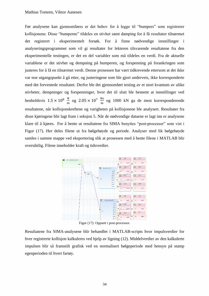
disse kjøringene blir lagt fram i seksjon 5. Når de nødvendige dataene er lagt inn er analysene

klare til å kjøres. For å hente ut resultatene fra SIMA benyttes “post-processor” som vist i

Figur (17). Her deles filene ut fra bølgehøyde og periode. Analyser med lik bølgehøyde

samles i samme mappe ved eksportering slik at prosessen med å hente filene i MATLAB blir

oversiktlig. Filene inneholder kraft og tidsverdier.

Figur (17): Oppsett i post-processor.

Resultatene fra SIMA-analysene blir behandlet i MATLAB-scripts hvor impulsverdier for

hver registrerte kollisjon kalkuleres ved hjelp av ligning (12). Middelverdier av den kalkulerte

impulsen blir så framstilt grafisk ved en normalisert bølgeperiode med hensyn på stamp

egenperioden til hvert fartøy.


35

5. Introduksjon til artikkel

Artikkelen er gjort i kollaborasjon med en annen gruppe som har fokus på eksperimentell

testing av hvordan retningsendring påvirker oppstående bøyemoment og kollisjonskreftene

mellom lekter og vindturbin. Begge oppgavene bygger videre på tidligere eksperimentelle

prosjekter [6] og [7], derfor presenteres resultatene på samme format som disse artiklene med

eksperimentelle og numeriske resultater. I denne artikkelen presenteres en introduksjon til

oppgaven og grunnlag for hvorfor den gjennomføres, eksperimentelt oppsett og

gjennomførelse, hvilke numeriske innstillinger som er benyttet i programvaren for

installasjons-fartøyene og vindturbinen, og hvorfor disse er valgt. Deretter vil resultatene som

er opparbeidet ved eksperimentell testing og numeriske analyser presenteres, og

sammenlignes med tidligere resultater. Oppgaven vil til slutt oppsummeres, hvor det

diskuteres for videre testing.

Investigation into the loads occurring between a floating offshore windturbine and an installation vessel

D. Ekerhovda, S. Bogea, M. Tomrena, V. Aanesena, T.C. Thuestada, D. Lande-Sudalla,∗

aWestern Norway University of Applied Sciences, Department of Mechanical and Marine Engineering, Inndalsveien 28,5063 Bergen. Norway

Abstract

Floating wind turbines (FWTs) utilizing spar-buoy platforms have proven to be a feasible solution to harness

clean energy from offshore wind. A downside to the spar-buoy concept is the significant draught needed to

maintain stability, which in turn reduces the number of possible quayside assembly and installation loca-

tions. Previous work investigating a possible draught reduction of the floating wind turbine using a barge

type installation vessel in irregular head seas is continued here for irregular following seas; where the turbine

is lying the wake of the barge. Overturning moments between the barge and FWT are measured experi-

mentally, and for following seas, the loads on the mechanical linkage between barge and FWT are found to

be greater than previously reported results in head seas. Collisions between the barge and FWT have also

been investigated in regular following waves. Using this wave direction the collision forces are significantly

reduced compared to previous results in regular head waves and most of the results are within the relevant

existing design standards. A numerical model, developed in DNV-GL’s Sesam package and validated against

the experimental results, is used to examine if a vessel with semi-submersible properties can reduce the mag-

nitude of the possible collision forces. Both wave directions are examined in the numerical work with results

showing a reduction in mean collision impulse between 35-66% when using a vessel with semi-submersible

properties, depending on test parameters, such as wave height, wave period and wave direction.

Keywords: Floating, offshore wind, installation vessel, collision, load modelling

∗Corresponding authorEmail address: [email protected] (D. Lande-Sudall)

1

1. Introduction

Governments have a unique opportunity to aide a new era for global climate action with economic

stimulus packages to confront the COVID-19 crisis [1]. By investing in development, deployment and

integration of clean energy technologies a twin beneficial situation is achieved where economies are stimulated

and the transition to clean energy sources is accelerated [1]. One of the industries with potential to meet

this aim is offshore wind. Offshore wind has the potential to generate more than 420 000 TWh per year

world wide, equivalent to more than 18 times the global electricity demand today [2]. Approximately 80% of

this potential is located in ocean areas with water depths exceeding 60 m, where the resource is greater and

less turbulent [3]. Fixed-bed foundations for offshore wind turbines become less economically viable with

increasing depth due to excessive material usage per MW installed capacity [4], and so there is significant

interest to utilise floating platforms. Multiple floating concepts are currently in development, and one of

the leading companies is Equinor with their Hywind concept utilising a spar-buoy platform. Their pilot

project Hywind Scotland has been operational since 2017 and features five, 6 MW floating wind turbines,

providing electrical power equivalent to the consumption of 36 000 households [3]. The turbines for Hywind

Scotland are assembled in a deep water fjord just outside of Stord, Norway, utilising the world’s largest

floating crane, Saipem 7000. A challenge with the spar-buoy platform is the large draft of the buoy, which

for Hywind Scotland is over 70 m. This limits the number of available ports for turbine assembly, due to

the low number of ports with such deep waters, and deep enough transit routes out to the production site.

A second challenge with the assembly of the turbines is the use of specialist floating crane vessels, which

will become less available when multiple wind parks are to be completed in different locations. Numerous

assembly methods are currently being investigated, in order to make the spar-buoy concept more accessible.

In 2014 Equinor held an ‘Innovation Challenge‘, where different installation concepts were presented. Among

the participants were the three winning companies; MODEC, Ulstein and Atkins [5]. MODEC and Ulstein

both have a method based on a transportation vessel that transports ready assembled turbines out to the

production site and mounted on the preinstalled spar-buoy platform. The methods are distinguishable by

a different connection method between the turbine tower and the spar-buoy. The proposal from Atkins is

a reusable transportation frame for up to four turbines. The method reduces the draft of the spar-buoy

and gives an increased stability when the four turbines are connected to the frame. The reduced draft also

gives the possibility for quayside assembly, which removes the need for floating crane vessels. The method

presented by Atkins was the source of inspiration for an earlier masters thesis [6] and a subsequent conference

paper [7]. Here, overturning moments and possible collision loads in the mechanical linkage between the

frame and turbine induced by met-ocean conditions during tow-out and installation at site were evaluated.

The work presented herein is a continuation of the work done in these projects and is divided into two parts;

an experimental part and a numerical modelling part.

2

The experimental method employs the same lab-setup used in previous testing, but with some modifica-

tions on the mooring system, and with opposite wave direction. The aim is to investigate if a change in wave

heading will alter the magnitude of the overturning moments and possible collision forces between the vessel

and floating wind turbine (FWT), further the numerical model examines if a vessel with semi-submersible

properties can reduce the magnitude of the possible collision forces. To achieve these aims, the following

steps have been conducted:

• Connected FWT-vessel in irregular JONSWAP spectra with significant wave height HS = 1.5 m,

HS = 2 m and peak spectral period TP between 6.5-16.5 s

• Collision impulse between disconnected FWT and barge under regular waves with wave height, H = 1.5 m

and period, T , varied between 6.5-16.5 s

• Collision impulse between disconnected FWT and semi-submersible vessels under regular waves with

wave height, H = 1.5 m, H = 2.9 m and period, T , varied between 6.5-22 s

The experimental and numerical methods employed are presented in Section 2. Section 3 evaluates

the results for magnitude and occurrence of overturning moments between the connected vessel and wind

turbine. Section 4 evaluates the possible impulse loads occurring during separation of the wind turbine from

the vessel. Section 5 presents the main conclusions from the work along with suggestions for future work.

2. Method

2.1. Test matrix

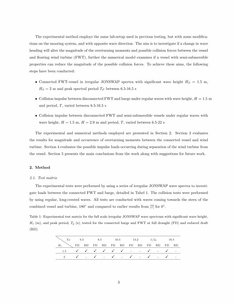
The experimental tests were performed by using a series of irregular JONSWAP wave spectra to investi-

gate loads between the connected FWT and barge, detailed in Tabel 1. The collision tests were performed

by using regular, long-crested waves. All tests are conducted with waves coming towards the stern of the

combined vessel and turbine, 180◦ and compared to earlier results from [7] for 0◦.

Table 1: Experimental test matrix for the full scale irregular JONSWAP wave spectrum with significant wave height,

Hs (m), and peak period, Tp (s), tested for the connected barge and FWT at full draught (FD) and reduced draft

(RD).

Hs

TP 6.5 8.5 10.5 13.2 1/f0 16.5

FD RD FD RD FD RD FD RD FD RD FD RD

1.5 ! ! ! ! ! ! - - ! - ! -

2 ! - ! - ! - ! - ! - ! -

3

Table 2: Experimental test matrix for full scale regular sinusoidal wave parameters wave height, H (m), and period,

T (s), of the barge and full draught FWT. Each time-series was conducted with a minimum of seven repetitions.

H

T6.5 8.5 10.5 13.2 1/f0 16.5

1.5 ! ! ! ! ! !

The numerical cases are for the same sea-states as the experimental tests as well as an additional case

for the eigenperiod of the new installation vessels. The numerical cases are performed with waves coming in

towards the bow (0◦) and the stern (180◦). Testing involves four different installation vessels, a numerical

version of the experimental barge and three vessels with semi submersible properties, referred to as new

vessel 1 (NV-1) with 6 equal columns, new vessel 2 (NV-2) has removed the center columns and new vessel

3 (NV-3) have narrower columns than NV-1. The eigenperiod varies with each vessel, as shown in Table 3 .

The second period is changed from 8.5 s to 9 s as that is the pitch eigenperiod for installation vessels with

semi-submersible properties. The advantage with numerical simulations is that there is no load-capacity

limit on mechanical load cells to impede testing higher periods. Therefore more tests have been performed

on the barge-like vessel in simulation than for experimental tests.

Table 3: Numerical test matrix for full scale regular wave spectrum with wave height, H (m), and period, T (s) for

connected installation vessels and full draught FWT.

H

T6.5 9 10.5 12.3 13.2 13.7 14.8 16.5 18/20/22

1.5 ! ! ! ! ! ! ! ! !

2.9 ! ! ! ! ! ! ! ! !

2.2. Experimental Method

All the experimental tests have been performed in the MarinLab towing tank at the Western Norway

University of Applied Sciences. This has a length, width and depth dimensions of 50 m, 3 m and 2.2 m

respectively, and is equipped with a six-flap Edinburgh Designs wavemaker with force feedback. A four

camera Qualisys motion-capture system is focused at the center of the tank with sampling frequency of

150 Hz. In order to compare the results from a wave heading of 180◦ with previous results at 0◦ [7], the

same barge-type vessel and floating wind turbine (FWT) as used in [7] are utilized. This involves testing

with a single floating wind turbine, (FWT) and a barge, as opposed to the semi-submersible model with

multiple turbines presented by Atkins, which simplifies testing.

4

The overall dimensions of the barge and FWT are given in Table 5 and these have been Froude-scaled

from full-scale dimensions given in [6] and [7] respectively using a 1:72 geometric scaling factor. The geometry

of the scaled FWT is simplified from the conical hywind shape at the waterline to a cylinder with a constant

diameter of D=0.2 m. The reduced draught model FWT is 18% shallower than the full draught. This is less

than the expected 30% reduction in draught at full scale, due to material limitations of the test model [6].

Some minor changes to the mooring system were implemented compared to the previous tests. Both vessels

were lightly moored to the tank walls using pulleys at the far end so that the mooring lines could be more

easily adjusted from one end. The barge is attached with two lines to both the starboard and port sides in the

bow and rear with an approximate 45◦ angle from the tank walls. For the FWT, two lines are attached with

a 90◦ angle with the tank walls. Each line is equipped with two springs in serial which results in a combined

stiffness of 98 N/m per line. The mooring lines are pre-tensioned to both the barge and FWT just before the

springs start to act. The camera system was used to verify that the global position of the combined barge

floating wind turbine (BFWT) was centered in the tank. In order to measure the wave elevation during

the experiments, resistance-type wave gauges are used. At the model, two wave gauges (analog and digital

signals) were placed in a parallel at the upstream position for synchronisation. To capture undisturbed wave

signal, a wave gauge with a digital signal, is placed 10 m in front of the model. The experimental setup are

shown in Figure 1. The digital wave gauge signals are recorded at 128 Hz, whilst the analogue wave gauge

and load cell signals are recorded at 2000 Hz. All wave gauges are calibrated using a three-point calibration

at different depths. To measure the horizontal collision loads and overturning moments about the deck, a

load cell rig consisting of two tension/compression load cells (one Applied Measurements DDEN 250 N and

one HBM U9C 500 N capacity) was fitted to the barge. In addition to the load cells, two electromagnets

(12V RS Pro EM80) were also mounted on the load cell rig and automated in LabView to control the release

of the FWT from the barge during the experiments.

Figure 1: Experimental setup of the barge and FWT connected in the wave tank, with mooring lines, wave gauges

and reflectors.

5

2.2.1. Load cell calibration

To measure the collision loads and overturning moments between the model scaled barge and FWT, a

load cell rig is mounted on the barge which is designed to prevent off-axis loading. Each of the two load cells

are calibrated by applying five loads varying from 0-200 N for both tension and compression. The load cells

are thereafter calibrated whilst assembled on the rig, also here with loads varying from 0-200 N, at three

distances, one in center and two at the sides of the loading plate shown in Figure 2 (a). From Figure 2 (b)

the rig behaves linearly, with the step-change at 0 N load occurring due to the weight change of the device

when orientated for tension and compression. This step is removed by applying a zero-load offset before

each test commences.

(a) (b)

Figure 2: (a) Load cell rig calibration in compression, with three load positions across the loading plate measured

from the center. (b) Calibration curves of the upper load cell (ULC) with five loads varying from 0-200 N tension

( •) and compression ( ◦) applied at F2.

6

2.2.2. Wave calibration

To ensure that the wavemaker generates an accurate theoretical irregular JONSWAP spectra, all wave

data captured from the wave gauges is processed through Edinburgh Design’s wave generating software,

Njord Synthesis [8]. A gain correction is applied after measuring each wave spectra for a 20 minute period

without the model, in order to remove the residual difference between the measured spectral energy, Sxx,

generated by the wavemaker and theoretical spectra across all frequencies, f . As shown in Figure 3, the

measured spectral energy from the wave gauges after a gain correction is applied, agrees well with the

theoretical JONSWAP spectra. It should be noted that the maximum frequency cut-out for the wavemaker

is limited to 2 Hz.

Figure 3: Comparison of the measured, gain corrected wave spectra (black) and the theoretical JONSWAP wave

spectra (blue), for Hs=1.5 m and Tp=1/f0 s ( ), Hs=2 m and Tp=8.5 s ( ). The wave frequency is normalized

against the full draught BFWT eigenfrequency, f0.

2.2.3. Decay testing

Decay tests have been conducted for the barge, the turbine and for the BFWT, for the pitch and roll

rotation. The purpose of the decay test is to observe the natural, free decay of each body and allow the

theoretical eigenperiod to be compared to the experimental eigenperiod measured in the tests. It is thus

possible to identify how much the mooring system affects the vessel response and also calculate the damping

coefficient of the different bodies. The eigenperiods and the damping coefficients are presented in Table 4.

The decay test is performed by applying an initial displacement to the body so that it begins to oscillate.

The displacement is applied manually, so the same decay test is performed several times to obtain a repeat-

able average. A decay test in surge has also been conducted, but is only used to evaluate the stiffness of the

7

mooring system. The FWT with a reduced draught was too unstable due to a negative metacentric height,

therefore no decay tests were conducted for this case.

The natural periods and damping ratios were found by the least squares method with an exponential

sinusoidal decay curve, (1) [7]. As shown in Figure 4 there is a excellent similarity between the experimental

data and the curve fit.

yn = A sin(√

1− ζ2ω0t+ φ)e−ζω0t (1)

In equation (1), A is the initial magnitude of the oscillation curve, ζ is the damping ratio, ω0 = 2πf0

the natural un-damped frequency and φ is the phase angle at some arbitrary point [7]. Decay tests in heave

were only conducted for the FWT, since the heave response for the barge and the BFWT is highly damped,

and therefore it is not possible to obtain an accurate natural period and a damping ratio. The same applies

to the decay test for the barge, because of the large waterline area, the barge acts like a overdamped system

so there are too few oscillations from which to obtain accurate estimates of frequency and damping ratio.

Figure 4: The experimental data ( ) and the belonging curve fit ( ) for the decay of the FWT in pitch.

Table 4: Presentation of the natural periods in full-scale, 1/f0(s), and the damping ratio, ζ , for the barge, FWT

and the BFOWT at full and reduced draught.

ModeB FWTFD BFWTFD BFWTRD

s [-] s [-] s [-] s [-]

Heave - - 18.11 0.017 - - - -

Pitch 7.9 0.251 36.972 0.05 13.7 0.039 13.05 0.032

Roll 6.65 0.112 34.3 0.016 20.04 0.01 22.72 0.015

Surge 61.42 0.113 835.28 0.159 163.74 0.07 132.68 0.091

8

2.3. Numerical method

The numerical analysis of collision loads between the installation vessel and FWT is performed using

DNV-GL’s offshore structural engineering software, Sesam. Four different numerical models (shown in

Figure 5) of the installation vessel have been created, where one is similar to the barge-type vessel used in

the experimental method and specified with dimensions detailed in Høyven [6]. The other three models are

different variations of a new installation vessel concept with semi-submersible characteristics. A numerical

model of the FWT is created from the full-scale Hywind turbine dimensions from [9], with the rotor and

nacelle assembly (RNA) represented by a point mass. An appropriate plate thickness is added to each vessel

structure and to the FWT’s substructure to include the mass of these in the structure model, remaining

mass of solid and liquid ballast is added separately in the hydrodynamic analysis (see Section 2.3.1). All

models are modeled using Sesam’s sub-program GeniE. Weight of the models is displayed in Table 5 along

with main dimensions.

Table 5: Main dimensions and particulars of the barge, NV-1, NV-2, NV-3 and FWT in full and model scales. Values

in brackets () indicate reduced draught dimensions and values with respective symbols, are the new displacement mass

and draught, due to modifications to the barge. Where (*)=1.27×107 kg, (?)=33.25 kg, (◦)=0.0543 kg, (�)=3.91

m, (�)=3.74 m and (∗)=0.0519 m.

Particular, unit Barge NV-1 NV-2 NV-3 FWT

full model full full full full model

Overall length, m 100 1.389 62 62 62 - -

Beam, m 37 0.514 42 42 42 - -

Diameter, m - - - - - 14.4 0.2

Draught, m 4 � 0.056 ◦ 13 13 13 76 1.06 (0.86)

Displacement mass,

kg1.30×107 * 33.85 ? 1.15×107 1.05×107 1.10×107 1.15×107 30.06

Top head mass, kg - - - - - 3.6×105 0.94

Centre of gravity

above keel, m3.77 � 0.052 ∗ 8.93 8.67 8.77 26.42 0.367 (0.507)

(a) (b) (c) (d)

Figure 5: Numerical models - NV-1 (a), NV-2 (b), NV-3 (c) and the numerical barge (d)

9

2.3.1. Hydrodynamic analysis

Hydrodynamic analysis of the numeric models are executed in HydroD. HydroD uses Wadam to calcu-

late the frequency domain wave loads analysis at zero speeds. The software calculates the hydrodynamic

coefficients by diffraction and Morison theory [10]. For its calculations, Wadam differentiate between three

methods; Morison equation for slim structures, first and second order potential theory for structures with

a large volume or a combination of both mentioned methods if the structure incorporate slim and large

structured sections. A mesh is applied in Genie to generate the panel model and structure model. The

tetrahedral mesh covers the outer area of the chosen structure. Different sizes of mesh are applied to the

panel model and structure model. The reason for the difference in mesh size is due to the computational

capacity required to run the analysis. The panel model is the wet surface structure used for hydrodynamic

calculations and so a finer mesh is desirable. A finer mesh size results in more accurate calculation (within

the limit of potential flow theory), but computational expense increases. The Panel model also provides an

expression for added mass and damping. To describe this geometry, a quadrilateral mesh is applied. The

structure model contains everything of the model to simulate a mass matrix, which is used to calculate the

response of the vessel. A sensitivity study were run on NV-1 to decide if the applied panel model size was

appropriate. Mesh sizes of 0.5 m, 0.7 m and 1 m were tested as shown in Figure 6. Transfer functions in

heave and pitch showed no significant difference in accuracy, but the duration for generating the finer mesh

was considerably greater. The mesh sizes adopted for each model are shown in Table 6.

Table 6: Maximum mesh size for models used in numerical cases.

Structure/model Barge [m] NV-1 [m] NV-2 [m] NV-3 [m] FWT [m] BFWT [m]

Panel 1 0.7 0.7 0.7 1.5 1

Structure 1.5 1 1 1 2 1.5

A Morison model is added to include contributions from slender elements, and structural elements which

is in the boundary area between slender and large volume. Wave loads on slender elements is calculated

using Morison equation (2) and is added to the forces form the panel model. Elements that are in the

boundary area between slender and large volume is already included in the panel model and the mass

force contribution is added through this. However these elements may have a viscous contribution which

is included by Morison drag. Further, appropriate added mass and drag coefficients are assigned to the

different sections, see Table 7. These calculations are based on the Morison equation (2). By including a

Morison model, any external forces applied to the models, such as mooring lines and tethers are included in

a hydro model. The Morison model is combined from a set or sets of Morrison elements and are based on

two node beam elements and single nodes in a first level superelement generated by GeniE. The Morrison

elements are defined by assigning hydrodynamic properties to nodes and beam elements in HydroD [10].

10

Figure 6: Sensitivity study NV-1 - a) heave, b) pitch. Mesh size 0.5 m ( ), 0.7 m ( ) and 1 m ( )

There are several types of Morrison elements available to calculate hydrostatic and hydrodynamic effects,

but for these cases the 2D Morrison element calculations on wet surface are utilized. The coefficients are

chosen on the basis of cross section of elements, using look-up tables in DNV-RP-C205 [11]

Table 7: Coefficient for added mass and drag on pipe and box respectively

Name Cd,y Cd,z Ca,y Ca,z

Pipe 0.7 0.7 1 1

Box 1.9 2.4 1.6 1.43

F = ρCmV u˙ + 1/2 ρCdAu|u| (2)

All numerical models of the installation vessels use the structural model from GeniE as a mass model,

due to the plate thickness and material type that is applied. For the FWT, point masses are added in

HydroD for the solid and liquid ballasts along with a point mass for the turbine head. Remaining structural

mass for the FWT is included true the structure model. The FWT achieves the appropriate draft of 76 m.

A loading condition that results in a draft of 4 m and 13 m along with zero trim and heel are applied for the

barge and NV-types respectively. HydroD calculates the appropriate filling of the available compartments

to fulfill this loading condition. The compartments are filled with seawater with a density of 1025 kg/m3.

Results from the Hydrodynamic analysis is shared with SIMA, a marine operations analysis software, where

the collisions between the installation vessel and FWT are simulated and analysed.

11

Further work is done under the assumption that the numerical models of the installation vessel and FWT

are independent of each other, meaning no radiation force is present between the models during the SIMA

analysis.

2.3.2. Transfer functions

In HydroD the response amplitude operators (RAOs) for each NV are calculated. These are used to

assess in which wave period the vessel reaches its resonant frequency. Figure 7 shows the RAOs for all the

NV-models in heave and pitch. From Figure 7 (a) the largest response occurs for NV-3 with a peak nearly 3

times greater than the input wave height. Compared to NV-1 and NV-2 the response is unreasonably high

even though all vessels had the same specified data input when running the hydrodynamic analysis. Since

the response in heave does not affect the results of collision testing to a noticeable degree, no further effort is

spent on reducing this peak. In Figure 7 (b) the pitch curves are illustrated, and these demonstrate similar

response. NV-3 has a slightly higher peak than the other two.

(a) (b)

Figure 7: Response amplitude operator vs. normalised wave frequency, f/f0 for: a) heave [m/m] b) pitch [deg/m].

NV-1 ( ), NV-2 ( ) and NV-3 ( ).

12

2.3.3. Numerical collision analysis

The numerical testing in SIMA is divided into two different cases for each vessel; one where both objects

are moored and one where only the vessel is moored and the FWT is floating freely. The two test cases

are hereby referred to as test type 1 (TT1) and test type 2 (TT2) respectively. The purpose of TT1 is to

simulate the conditions in the experimental testing where both objects are lightly moored to the test basin

wall. This will cause the two objects to maintain a position where they will seek back together if they drift

apart. To simulate this motion in SIMA, the vessel is moored with four mooring lines with a pretension of

1000 kN, and the FWT with two lines of the same pretension. The lines are directed in 0◦ and 180◦ along

the x-axis due to little movement transverse to the wave direction. TT2 with the FWT floating freely serves

to simulate more realistic conditions where the vessel is held in place using dynamic positioning or similar

systems, and the FWT is released from the vessel. Another reason for conducting TT2 is to monitor what

effects the mooring of the FWT has on the collisions in TT1. The vessel in TT2 is moored using the same

method as in TT1. Both test types have the same environmental setup, with a water depth of 300 m and

wave variation as presented in the test matrix.

2.3.4. Specified mooring forces

Results of the hydrodynamic analysis should represent the vessel with the draft corresponding to the

loading condition, which includes all vertical components from the mooring forces. Vertical compensating

forces are included by adding specified forces equal to the vertical component of each mooring line. For each

mooring line a corresponding vertical force is inserted in the same coordinate as the respective body point

for that mooring line. Doing this ensures that the vessel has the correct draft for the SIMA analysis. Table

8 displays the magnitude of the specified vertical mooring forces applied to the different vessel types.

Table 8: Magnitude of vertical component of mooring line.

Model NV-1 NV-2 NV-3 FWT

Magnitude [N] 6.72×105 6.73×105 6.81×105 1.37×106

2.3.5. Bumper characteristics

Bumpers are added to the vessel and FWT to register the collision forces between the two. As the

stiffness of the load cell rig and model FWT has not been recorded, multiple analyses have been run to

find appropriate properties to assign the bumpers. Figure 8 and 9 show differences in impulse results for

multiple runs with a variation in bumper input. The impulse, I, is calculated for each collisions as the area

under the force-time curve, F, during the start t1 , and end t2, time of the collision [12], as shown in Figure

14 (b).

I =

∫ t2

t1

F (t)dt (3)

13

As seen in the figures, the run which gives results closest to the experimental results from the previous

work is chosen as a baseline and the properties from this run are used in the remaining analyses. From

Figure 8 (a), a high overall impulse force is found when no damping is applied to the bumpers, with high

impulse arising due to high impact forces despite a short duration of the impact. Furthermore, by analysing

multiple setups, a damping coefficient of 20.5 MNs/m is found to be an appropriate value in this setup.

Varying the stiffness values with this level of damping is compared to the results from the experimental

testing in Figure 8 (b), and some variations can be observed between them. The final combination is found

by investigating the collision forces and their duration. By applying a stiffness property of 150 MN/m,

along with the damping, a force distribution similar to the experimental work is found with results shown

in Figure 9. The other combinations shown in Figure 8 (b) resulted in collision forces that were significantly

grater than the forces found in the experimental work and were therefor excluded.

(a) (b)

Figure 8: Mean impulse, I, versus normalised wave frequency, f/f0 for wave height, H = 1.5 m and wave direction

0◦ for Barge with varying bumper stiffness and (a) no damping, (b) constant damping of 2.05×107 Ns/m.

Figure 9: Collision forces between the FWT and Barge versus impulse, with least-squares linear-fit ( ) through all

collisions (•), wave from 0◦ and H = 1.5 m from chosen stiffness at 1.5×108 N/m and damping 2.05×107 Ns/m

14

3. Moments between vessel and floating turbine

This section focuses at the overturning moments that occurs between the barge and the turbine in the

various irregular sea states, both at full and reduced draft.

3.1. Response amplitude operators of the connected vessel

The response amplitude operators (RAOs) in pitch for the BFWT, are obtained from the irregular sea

state test with Hs=1.5 m and Tp=10.5 s. The experimental RAOs are compared with a full scale and fully

drafted panel model in HydroD with mesh size 1 m, shown in Figure 10 (a). The numerical curves shows a

reasonable degree of resemblance to the experimental curve, especially at the peak response which is found

at the respective pitch eigenfrequency. The small deviations between the RAOs obtained by experiment

and HydroD are expected, especially given uncertainties in the experimental testing, as shown in Figure 10

(b). Such as those associated with having a finite test period and the ability of the wavemaker to generate

the exact theoretical spectrum. Similarly, the lack of accuracy in numerical modelling of viscous forces

also contributes to the discrepancies, especially around the pitch eigenfrequency where the viscous drag is

greatest. The peak response is greatest for the full draught BFWT in compassion to the reduced draught

BFWT.

(a) (b)

Figure 10: (a) Experimental response amplitude operator in pitch, deg/m response for the full ( ) and reduced

( ) draught BFWT, compared with a fully draught HydroD panel model (red). All RAO’s are obtained by

the square root of the respective response spectrum divided by input from the wave spectrum for Hs=1.5 m and

Tp=10.5 s. (b) Variation in experimental RAO’s obtained in different wave peak periods Tp=10.5 s, Tp=14.2 s and

Tp=16.5 s compared to HydroD panel model.

15

3.1.1. Overturning moments

The experiments where the barge and the FWT are connected, are performed with various irregular

JONSWAP spectra. The wave-induced forces are measured by the load cells on the load cell rig. From

the force measurements, the bending moment are calculated around point P , as shown in Figure 11. The

bending moment, M , is calculated from equation (4).

M = Fd (4)

Where F is the force vector calculated from the load cells and d is the vertical distance from the point P

to the respective load cell. The total moment is then found by adding the bending moment from the upper

and lower load cell.

Figure 11: Side-view of the connected barge and FWT, showing how the force are acting on the load cells and the

distance from the barge deck to the lower and upper load cell [6].

3.1.2. Load occurrence statistics

The overturning moments from each time series are binned into 40 evenly distributed bins of overturning

moment magnitude, Figure 12 (a). The height of these bins indicates the probability that each of the different

moment intervals occur. A probability density function is then obtained using a method of least squares fit

from the normal distributed binned diagram. When comparing this probability function to the measured

data to each of the different seastates, it appears to be a excellent compliance for the occurring loads. For

the extreme values, there is some overestimation of the occurrence of the loads compared to the measured

data, as shown in Figure 12 (b). Since the time-series start at the same time as the wave-generator starts,

the irregular sea-states are not fully developed in the beginning, because of this, the start of the time-series

is removed from each dataset to remove the distortion this would create to the otherwise normal distribution

of the occurring moments.

16

(a) (b)

Figure 12: Probability density function ( ) of the normal distributed binned histogram (a) and the corresponding

measured data ( ) plotted against the standard normal distribution (b) for Tp = 10.5 s and Hs = 1.5 m with a

wave heading at 180◦.

To evaluate the most extreme values of the occurring moments, three standard deviations (3σ) which

represents a 99.7% probability interval, is shown in Figure 13 for each sea-state and with full and reduced

draught. These standard deviations are shown for wave headings at both 0◦ and 180◦. As expected, there

is an increase in load as the significant wave height increases, which is greatest about the natural pitch

frequency for the connected BFWT, where max (3σ)=0.92 GNm at Hs=1.5 m and max (3σ)=1.45 GNm

at Hs=2 m, with a wave heading at 180◦. However the bending moments are consistently higher for 180◦,

especially with increasing significant wave height. It is also seen that the loads are consistently higher when

the FWT has a reduced draught with a wave heading at 180◦.

Furthermore, it can be observed from Figure 13 that the loads at a significant wave height of 2 m are

almost the same magnitude as the wave height of 3.5 m. This may be due to the fact that there was water

floating on deck during the experiments at a significant wave height of 3.5 m. This causes a free surface

effect which can attenuate the movement of the system, and the measured bending moments could therefore

be lower than they should be, had the vessel had a greater freeboard and no water on deck. From the

decay tests, the connected bodies were shown to be an underdamped system in pitch, which may explain the

rapidly increasing loads around the pitch eigenfrequency as the system is unable to dampen out its motions

in pitch to any particular degree. A contributing factor to this may be the simplification done of the scaled

turbine, where the coned part of the substructure is ignored. It is assumed that the coned geometry will

dampen the coupled heave and pitch response, but after running numerical analysis in HydroD, it is found

that there is almost no difference in the pitch and heave response with and without the coned geometry for

the connected barge and turbine.

17

Figure 13: Normalised peak overturning moment (3σ/max{3σ}) versus wave frequency, f/f0 with Hs=1.5 m (�),

Hs=2 m (×) and Hs=3.5 m (◦), for the full draught ( , filled markers) and reduced draught ( , open markers)

for waveheadings 180◦ (blue) and 0◦ (black). Here, max{3σ}=1.49 GNm, in full-scale.

4. Collision load results

Regular waves were used during the collision tests for both the experimental and numerical method.

Coordinate system is equal for the two methods, with waves from 0 and 180◦ indicating waves propagating

towards the bow or stern respectively.

4.1. Experimental collision loads

For each of the sea states mentioned in Table 2, seven repetitions were performed such that the mean

impulse could be calculated. Depending on the sea state, 2-7 collisions occurred during each time series.

However it proved difficult predicting when the collisions were to occur, due to the light mooring system

which will not be presented at full scale. When releasing the FWT, some collision may occur in the early

release phase, otherwise the vessels seems to drift naturally apart, and thus no collisions would be expected

to occur. However, as an effect of the light moorings the barge and FWT are forced back together due to

their respective eigenperiods in surge, given in Table 4. As a result of this, these collisions impacts could

measure a possible worst case scenario when interacting in different sea states.

When releasing the FWT from the barge, the release phase of the electromagnets was randomly set

during the experiments, except for the collision tests conducted with wave period the same as the pitch

eigenperiod of the BFWT. The electromagnets were not able to hold the turbine during this wave set, which

18

led to releasing just before the magnets startet to slipp. According to [6] and [7] the release phase of the

electromagnets relative to the wave phase showed to have no significant correlation to the magnitude of the

collision impulse. During the experiment, the electromagnets was set to release the FWT for a period of 60

seconds for each time series before connecting it back on to the load cell rig, as shown i Figure 14 (a)

(a) (b)

Figure 14: (a) Model scale force-time series with occurring collisions ( ) for H = 1.5 m and T = 10.5 s, showing

magnet release point ( ). (b) The area between curve and x-axis is used to obtain the impulse, I, of the first

collision from (a).

Figure 15 (a) shows that the maximum collision impulse with wave heading 180◦, is reduced significantly,

by 47% when comparing to the wave heading at 0◦. Furthermore the shape of the curves during the higher

wave frequencies can be observed as to be quite similar for both wave headings. As a result of this, the

collision test with the turbine lying in the barges wake shows an improvement in reducing the collision

impulses, however it is still advantageous to operate in shorter wave periods than the pitch eigenperiod of

the BFWT. To measure the collision forces a vessels is to withstand when interacting with the FWT, all the

collision forces are plotted against the corresponding impulses in Figure 15 (b). According to [13], the surface

area between the barge and FWT is designed to withstand a force of 2.5 times the mass displacement of the

barge, which in this case is 32.4 MN. From Figure 15 (b) the majority of the collision forces lies beneath

the design force level, however there are some collisions extending this level which correlates with the wave

periods close to the eigenperiod of the BFWT.

19

(a) (b)

Figure 15: (a) Variations in full scaled impulse loads, I, with normalized wave frequency f/f0 for wave

height, H = 1.5 m. Wave direction 180◦ (mean: and max: ) compared with wave direction 0◦ (mean:

and max: ) from previous results [7]. (b) Collision forces between the FWT and barge versus impulse, with least-

squares linear-fit ( ) through all collisions (•). Maximum collision forces from each regular wave set of H = 1.5 m

and T = 6.5 (◦), 8.5 (+), 10.5 (�), 13.2 (×), 14.2(∆) s.

4.2. Numerical collisions loads

Results from the numerical analysis are presented in this section and are divided accordingly to the two test

types, TT1 and TT2, presented earlier. Regular waves are used for both test types with values presented in

Table 3.

TT1 - Moored wind turbine and barge

Due to the mooring of the vessel and FWT, the numerical method experienced similar challenges as

the experimental tests with regards to selecting which collisions to include in the calculations. Therefore

a window of 100 s is used where all collisions from t = 0 s and to t = 100 s are included and the collision

impacts measure a possible worst case scenario when interacting in different sea states.

Figure 16 shows an average 65% reduction of mean collision impulse between the NV-models and the

numerical barge type vessel with wave height, H = 1.5 m and waves from 0◦. Comparable results are found

with an average reduction of 66% with wave height, H = 2.9 m. Similar to [7] impulse for H = 1.5 m is

around 50-60% of that measured for H = 2.9 m stating that operations of this kind should be conducted in

conditions with a low wave height to reduce the risk of collisions with high impulse load. When comparing

with experimental results for 0◦ and H = 1.5 m, the mean impulse value for the NV-types is found to

be of a similar magnitude, with experimental results showing a somewhat greater peak value of the mean

20

impulse. The larger impulse values for the numerical barge compared to experiment is due to longer lasting

collisions in the numerical work, resulting in a larger integration area. This may suggest that the stiffness or

damping of the numerical bumper is not right, and ideally measures from a free-decay test of the load cell

rig would be used. A different behavior is observed in both plots for the NV-2 model, due to the removal

of the two mid columns it seems to have gained other properties at the lower wave periods, with the peak

mean value at a wave period of 6.5 s. Lower wave periods should be tested to locate the peak value for NV-2.

Figure 17 (a) and (b) compares the impulse to the corresponding peak force from each collision with

H = 1.5 m and H = 2.9 m for NV1-3 with waves at 0◦. The contact area between the vessel and FWT is

required to withstand 27.5 MN on average between the three NV-models [13]. Figure 17 (a) shows that all

collisions with H = 1.5 m are below this design load by nearly 10 MN, furthermore for Figure 17 (b) only

a few collisions exceed this limit with H = 2.9 m. When comparing the collision forces from [7] with the

collision forces for the NV-types, a lower overall force is found for the NV-type with H = 1.5 m.

Figure 16: Mean impulse loads, I, with normalized wave frequency f/f0 for each vessels pitch eigenfrequency , wave

height H = 1.5 m ( ) and H = 2.9 m ( ), Wave direction 0◦ for Barge ( / (numerical) (experimental))

and NV1-3 ( / (1) / (2) / (3)).

21

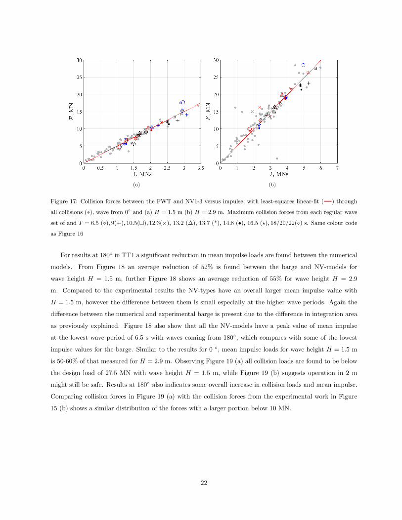
(a) (b)

Figure 17: Collision forces between the FWT and NV1-3 versus impulse, with least-squares linear-fit ( ) through

all collisions (•), wave from 0◦ and (a) H = 1.5 m (b) H = 2.9 m. Maximum collision forces from each regular wave

set of and T = 6.5 (◦), 9(+), 10.5(�), 12.3(×), 13.2 (∆), 13.7 (*), 14.8 (•), 16.5 (?), 18/20/22(�) s. Same colour code

as Figure 16

For results at 180◦ in TT1 a significant reduction in mean impulse loads are found between the numerical

models. From Figure 18 an average reduction of 52% is found between the barge and NV-models for

wave height H = 1.5 m, further Figure 18 shows an average reduction of 55% for wave height H = 2.9

m. Compared to the experimental results the NV-types have an overall larger mean impulse value with

H = 1.5 m, however the difference between them is small especially at the higher wave periods. Again the

difference between the numerical and experimental barge is present due to the difference in integration area

as previously explained. Figure 18 also show that all the NV-models have a peak value of mean impulse

at the lowest wave period of 6.5 s with waves coming from 180◦, which compares with some of the lowest

impulse values for the barge. Similar to the results for 0 ◦, mean impulse loads for wave height H = 1.5 m

is 50-60% of that measured for H = 2.9 m. Observing Figure 19 (a) all collision loads are found to be below

the design load of 27.5 MN with wave height H = 1.5 m, while Figure 19 (b) suggests operation in 2 m

might still be safe. Results at 180◦ also indicates some overall increase in collision loads and mean impulse.

Comparing collision forces in Figure 19 (a) with the collision forces from the experimental work in Figure

15 (b) shows a similar distribution of the forces with a larger portion below 10 MN.

22

Figure 18: Mean impulse loads, I, with normalized wave frequency f/f0 for each vessels pitch eigenfrequency,

wave height H = 1.5 m ( ) and H = 2.9 m ( ), Wave direction 180◦ for Barge ( / (numerical)

(experimental)) and NV1-3 ( / (1) / (2) / (3)).

(a) (b)


all collisions (•), wave from 180 degrees and (a) H = 1.5 m (b) H = 2.9 m. Maximum collision forces from each

regular wave set and T = 6.5 (◦), 9(+), 10.5(�), 12.3(×), 13.2 (∆), 13.7 (*), 14.8 (•), 16.5 (?), 18/20/22(�) s. Same

colour code as Figure 18

23

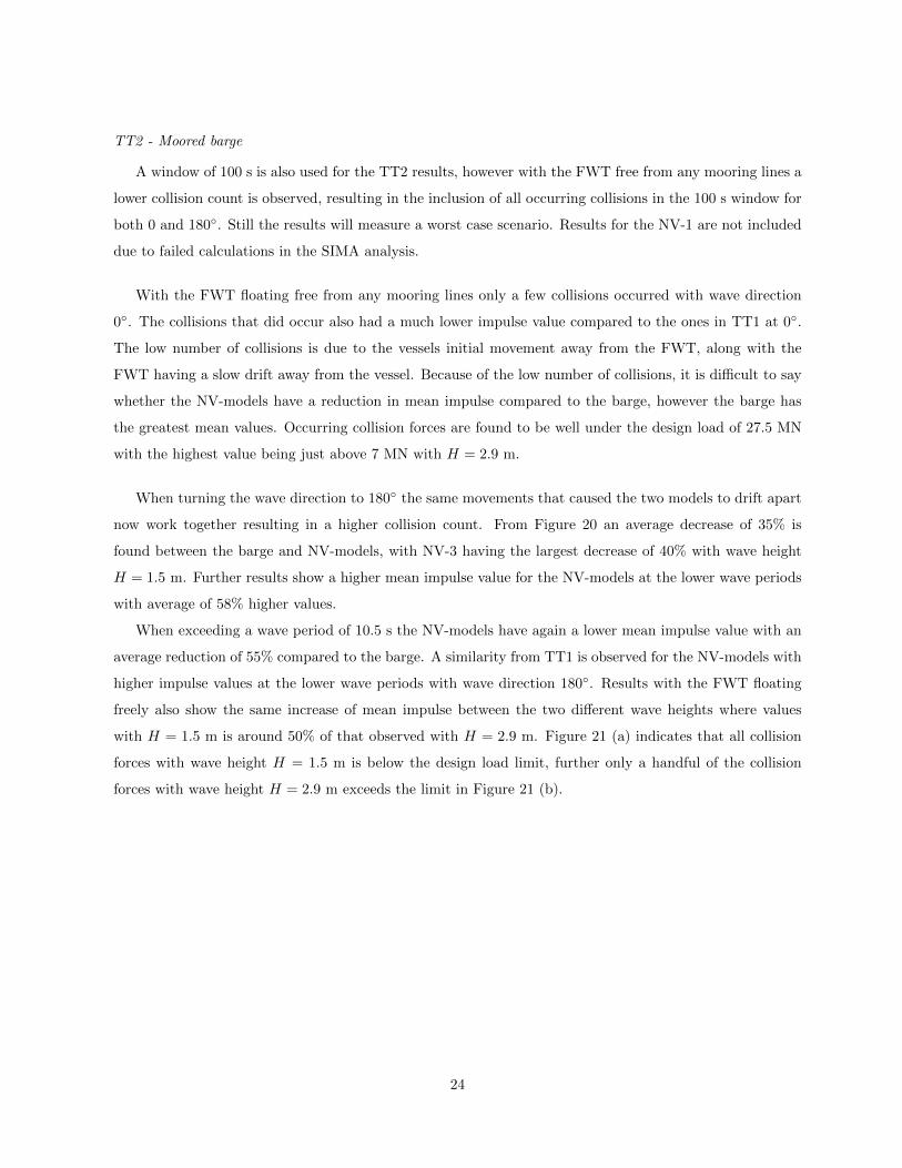
TT2 - Moored barge

A window of 100 s is also used for the TT2 results, however with the FWT free from any mooring lines a

lower collision count is observed, resulting in the inclusion of all occurring collisions in the 100 s window for

both 0 and 180◦. Still the results will measure a worst case scenario. Results for the NV-1 are not included

due to failed calculations in the SIMA analysis.

With the FWT floating free from any mooring lines only a few collisions occurred with wave direction

0◦. The collisions that did occur also had a much lower impulse value compared to the ones in TT1 at 0◦.

The low number of collisions is due to the vessels initial movement away from the FWT, along with the

FWT having a slow drift away from the vessel. Because of the low number of collisions, it is difficult to say

whether the NV-models have a reduction in mean impulse compared to the barge, however the barge has

the greatest mean values. Occurring collision forces are found to be well under the design load of 27.5 MN

with the highest value being just above 7 MN with H = 2.9 m.

When turning the wave direction to 180◦ the same movements that caused the two models to drift apart

now work together resulting in a higher collision count. From Figure 20 an average decrease of 35% is

found between the barge and NV-models, with NV-3 having the largest decrease of 40% with wave height

H = 1.5 m. Further results show a higher mean impulse value for the NV-models at the lower wave periods

with average of 58% higher values.

When exceeding a wave period of 10.5 s the NV-models have again a lower mean impulse value with an

average reduction of 55% compared to the barge. A similarity from TT1 is observed for the NV-models with

higher impulse values at the lower wave periods with wave direction 180◦. Results with the FWT floating

freely also show the same increase of mean impulse between the two different wave heights where values

with H = 1.5 m is around 50% of that observed with H = 2.9 m. Figure 21 (a) indicates that all collision

forces with wave height H = 1.5 m is below the design load limit, further only a handful of the collision

forces with wave height H = 2.9 m exceeds the limit in Figure 21 (b).

24

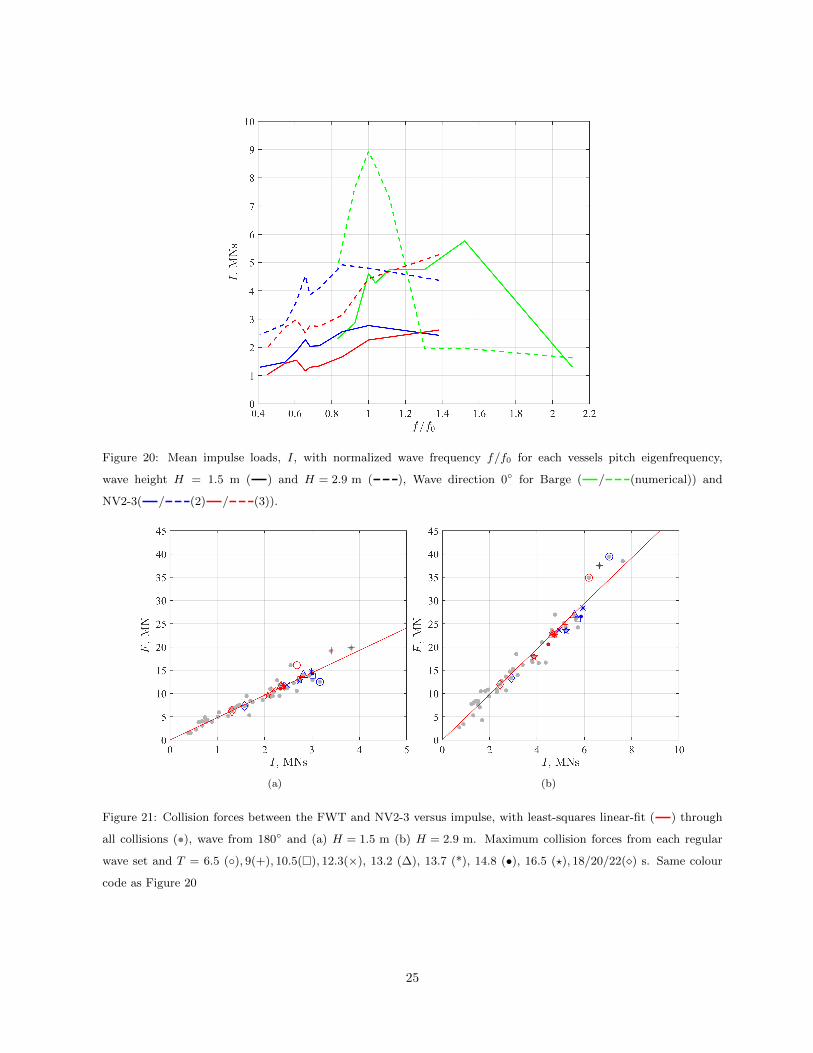
Figure 20: Mean impulse loads, I, with normalized wave frequency f/f0 for each vessels pitch eigenfrequency,

wave height H = 1.5 m ( ) and H = 2.9 m ( ), Wave direction 0◦ for Barge ( / (numerical)) and

NV2-3( / (2) / (3)).

(a) (b)


all collisions (•), wave from 180◦ and (a) H = 1.5 m (b) H = 2.9 m. Maximum collision forces from each regular

wave set and T = 6.5 (◦), 9(+), 10.5(�), 12.3(×), 13.2 (∆), 13.7 (*), 14.8 (•), 16.5 (?), 18/20/22(�) s. Same colour

code as Figure 20

25

5. Conclusion and future work

From the experimental tests using a JONSWAP wave spectra, a 15% increase in the peak overturning

moment around the pitch eigenfrequency of the BFWT, for the full draught case with a wave height at

Hs=1.5 m is found for waves from 180◦ compared to waves at 0◦. Furthermore, the overturning moments

shows a minor increase compared to a wave heading at 0◦ for all wave peak periods. It is also seen that the

loads increases as the significant wave height increases, especially around the eigenpriod of the BFWT. For

the reduced draught case with waves at 180◦, the overturning moments are consistently higher compared to

for waves at 0◦. As a result of this, it would be preferable, in terms of reducing loads on the mechanical

linkage, to operate with the reduced draught in head waves as opposed to following waves. Since the peak

overturning moments occured during the pitch eigenfrequncy of the combined BFWT, a vessel with lower

eigenfrecuency would be recommended.

Collision loads in regular waves were also investigated numerically and experimentally. For the experi-

mental tests, the collision loads with the turbine lying in the barges wake showed a significant reduction of

the max collision impulse with 47% compared to waves at 0◦. When considering the magnitude of collision

forces that the contact area between the barge and FWT would be required to withstand, waves at 180◦

reduces the majority of the collision forces below the level specified in existing design standards, compared

to loading in waves at 0◦ which regularly exceed this level.

However some of the collisions, corresponding to waves at the pitch eigenfrequency of the BWFT, exceed

this design limit and thus, it would still be advantageous to operate in higher wave frequencies than the

pitch eigenfrequency of the BFWT. As an effect of the light mooring system which will not be present at

full scale, the collisions proved difficult to predict. These collisions impacts could be used as a measurement

of a possible worst case scenario when interacting in different sea states.

Numerical analysis of the moored wind turbine and barge showed a reduction of mean collision impulse

with 65% on average between the numerical barge and the three NV-models with waves from 0◦. A further

52% reduction of mean collision impulse was found for waves at 180◦. When comparing results for the

numerical and experimental barge, mean collision impulse for the experimental results is found to be 35%

of that calculated in the numerical analysis, suggesting that the bumper setup may not have the correct

stiffness or damping characteristics. An other possible explanation is the assumption of no notable radiation

force between models. Analysis for the un-moored FWT resulted in a low collision count with a wave

direction of 0◦, with only three recorded collisions. However with a wave direction of 180◦, more collisions

were recorded and an average reduction of 35% in mean collision impulse by using the NV-models compared

to the barge, was found. With results for the NV-models showing a reduction in mean collision impulse

compared to the numerical barge it is reasonable to conclude that a vessel with semi-submersible properties

can reduce the magnitude of the possible collision forces between the vessel and FWT.

26

Future experimental work should focus on testing further irregular sea states and new off axis wave

directions. Testing a new vessel, such as one of the NV-models, with a lower pitch eigenfrequency could be

used to increase operationality in a wider range of sea-states. In addition to this, the acceleration of the

top-head mass could be investigated to assess limitations on loading of the turbine nacelle. The numerical

model should be further developed, focusing on a free-decay test of the load cell rig used in the experimental

method to determine appropriate damping and stiffness values to assign the bumpers used in the analysis.

Further a multi-body analysis with the FWT and NV-models should be done to include possible radiation

forces. Since regular waves rarely occur in real-seas, the collision loads and likelihood of occurrence for

irregular waves should be investigated, along with waves from off-axis directions.

27

References

[1] D. F. Birol. (2020) Put clean energy at the heart of stimulus plans to

counter the coronavirus crisis. [Online]. Available: https://www.iea.org/commentaries/

put-clean-energy-at-the-heart-of-stimulus-plans-to-counter-the-coronavirus-crisis

[2] IEA. (2019) Offshore wind outlook 2019. [Online]. Available: https://www.iea.org/reports/

offshore-wind-outlook-2019

[3] Equinor. (2020) We’re determined to be a global offshore wind energy major. here’s how. [Online].

Available: https://www.equinor.com/en/what-we-do/wind.html

[4] IRENA, “Floating foundations: a game changer for offshore wind power,” International Renewable

Energy Agency, Abu Dhabi, Tech. Rep., 2016.

[5] Equinor, “Hywind installation,” 2020. [Online]. Available: https://www.equinor.com/no/

how-and-why/innovate/the-hywind-challenge.html

[6] T. S. Høyven, “Bending moments and collision loads between a floating offshore wind turbine and a

supporting barge,” University of Bergen, 2019, master thesis.

[7] D. R. Lande-Sudall, “Wave-induced collision loads and moments between a spar-buoy floating wind

turbine and an installation vessel,” in DeepWind, 2020.

[8] E. Designs. (2016) Wave generating software. [Online]. Available: http://www4.edesign.co.uk/product/

wave-generating-software/

[9] T. I. Ulla, “Expanding into deeper waters: Development of the hywind floating wind concept,”

Sacramento, 2014. [Online]. Available: https://www.boem.gov/NREL-Expanding-Deeper-Waters/

[10] DNV-GL, WADAM - SESAM USER MANUAL, 2017.

[11] DNVGL, DNV-RP-C205 Environmental Conditions and Environmental Loads, 2014.

[12] S. N. Leksikon. (2018) Kraftstøt. [Online]. Available: https://snl.no/kraftst\%C3\%B8t

[13] DNVGL, DNVGL-ST-0119 Floating wind turbine structures, 2018.

28


36

6. Oppsummering og konklusjon

Det vil her presenteres en oppsummering av de numeriske funnene presentert i artikkelen.

Ved hjelp av funnene som er presentert vil det legges frem en konklusjon med fokus på å

svare på oppgavens problemstilling.

6.1 Oppsummering av funn

Resultatene vil bli oppsummert i henhold til de to ulike testsituasjonene, TT1 og TT2, som

presentert tidligere.

TT1 - Forankret fartøy og turbin

Fra analysene ved 0° og H = 1.5 m, ble det funnet en gjennomsnittlig reduksjon i

kollisjonenes impulsmiddelverdi på 65% mellom de tre NV-modellene og den numeriske

lekteren. Også ved bølgehøyde, H = 2.9 m, ble det funnet en betydelig reduksjon i impulsens

middelverdi som var på 66% gjennomsnittlig mellom NV-modellene og den numeriske

lekteren. Sammenligning av resultater for den numeriske og eksperimentelle lekteren viste at

de eksperimentelle verdiene lå på om lag 35% av det som ble målt for den numeriske. Dette

kan tyde på at de valgte verdiene for “bumpers”-innstillingene i SIMA ikke stemmer overens

med de fysiske verdiene for lastcellen benyttet i de eksperimentelle forsøkene. På grunn av

dette ble integrasjonsområdet ved beregning av de numeriske impulsverdiene større enn for de

eksperimentelle grunnet et lengre tidsintervall for de numeriske kollisjonene. Dette gjorde at

resultater for den eksperimentelle lekteren oppnådde omtrent like verdier som for de

numeriske NV-modellene og en eventuell reduksjon i impuls var ikke til stede. Ved en

endring av bølgeretningen til 180° ble det igjen funnet en gjennomsnittlig reduksjon på

impulsens middelverdi mellom NV-modellene og den numeriske lekteren på 52% og 55%

ved bølgehøyde, H = 1.5 m og H = 2.9 m henholdsvis. Igjen viste eksperimentelle verdier for

lekteren å ikke samsvare med de numeriske, trolig av samme årsak som nevnt tidligere.

Kontaktflaten mellom NV-modellene og turbinen skal kunne motstå en kraft på 27.5

MN, ifølge ligning (13). Ved observasjon av de opptredende kollisjonskreftene ved 0° og

180° i TT1 finnes alle kollisjonskrefter ved H= 1.5 m å være under denne designkraften.

Videre er det bare et fåtall av kollisjonene ved H = 2.9 m som har en kraft som overstiger en

verdi på 27.5 MN.


37

TT2 - Forankret fartøy Når den flytende vindturbinen ikke var forankret, oppsto kun et fåtall kollisjoner i analysene

med en bølgeretning på 0°. Kollisjonene som ble observert var også av en lavere størrelse enn

det som ble registrert ved 0° i TT1, med høyeste kollisjonskraft i overkant av 7 MN ved

H= 2.9 m. For analyser med bølgeretning 180° oppsto et større antall kollisjoner som ga

mulighet til å sammenligne de ulike modellene. Resultatene viste da en gjennomsnittlig

reduksjon i impuls middelverdi mellom den numeriske lekteren og NV-modellene på 35%

med H = 1.5 m, NV-3 oppnådde størst reduksjon på 40%. Med H = 2.9 m viste NV-

modellene å ha en høyere impuls middelverdi ved lavere bølgeperioder enn det som ble målt

for den numeriske lekteren. Gjennomsnittlig hadde NV-modellene i overkant av dobbelt så

høye impuls middelverdier ved lavere perioder. Når bølgeperioden oversteg en verdi på

10.5 s var det igjen NV-modellene som oppnådde den laveste impuls middelverdien med en

gjennomsnittlig reduksjon på 55% sammenlignet med den numeriske lekteren. Resultater fra

TT2 viser igjen at alle kollisjoner som oppsto ved H = 1.5 m resulterer i en kraft lavere enn

den beregnede designkraften på 27 MN, samtidig oversteg få av kollisjonene denne kraften

ved H = 2.9 m. Ved å se på forløpet til de ulike grafene for NV-modellene undersøkes det om

modellenes ulike utforming har hatt stor påvirkning på resultatene som er funnet. Det ses ikke

en markant forskjell mellom de ulike modellene i form av impuls middelverdi, da de ulike

modellene stort sett ligger i samme verdiområde. Det ses likevel et noe ulikt forløp i grafene

til NV-2, noe som er naturlig da det er denne som skiller seg mest fra de andre med kun fire

søyler.

6.2 Konklusjon

Målet med denne oppgaven var å undersøke om et installasjonsfartøy med egenskaper likt et

halvt nedsenkbart fartøy vil kunne resultere i en reduksjon av kollisjonskrefter mellom

installasjonsfartøyet og den flytende vindturbinen når den skal slippes løs fra fartøyet.

Konklusjonene som presenteres er basert på resultatene fra de ulike analysene som er kjørt.

Resultater fra TT1 og TT2 ga et godt innsyn i kollisjonenes størrelse og deres avhengighet av

bølgehøyde og retning. Fra analysene hvor vindturbinen ikke var forankret ble det vist at

sannsynligheten for at kollisjoner mellom installasjonsfartøyet og den flytende vindturbinen

er til stede, men med klart færre tilfeller med bølger i baug av fartøyet. Ved undersøkelse av

kollisjonenes impuls middelverdi viser numeriske verdier for den nye fartøystypen å ligge

godt under verdier som er funnet for lekter fartøyet ved de aller fleste tilfeller.


38

Den nye fartøystypen opplevde noe høyere impuls ved lavere perioder når vindturbinen ikke

var forankret. Verdier for impuls ved H= 1.5 m viste seg å være omtrent 50% av det som ble

målt for impuls med H= 2.9 m, noe som tilsier at det vil være fordelaktig å utføre denne type

operasjoner i sjøtilstander med lav bølgehøyde. Men grunnet det nye fartøyets bidrag i å

redusere kollisjonskrefter åpner det opp for at operasjonsgrenser med tanke på bølgehøyde

kan heves. Det nye fartøyet oppnådde en reduksjon på mellom 35-66% i impulsens

middelverdi sammenlignet med lekter fartøyet, avhengig av hvilken testsituasjon det ses på.

Det konkluderes derfor med at et fartøy med halvt nedsenkbare egenskaper vil føre til en

reduksjon av kollisjonskrefter mellom fartøyet og den flytende vindturbinen. Sammenligning

av numeriske og eksperimentelle verdier viste at impulsverdiene funnet for de numeriske

modellene ikke samsvarte med verdiene fra de eksperimentelle forsøkene. Høyere

impulsverdier ble funnet for de numeriske modellene grunnet kollisjoner med lengre durasjon

enn kollisjonene i de eksperimentelle forsøkene som resulterte i et større integrasjonsområde

når impuls ble beregnet. Dette kan være en indikasjon på at innstillingene for bumpers

benyttet i analysene ikke stemmer overens med egenskapene til lastcellen benyttet i lab-

forsøkene.

7. Fremtidig arbeid

For fremtidig arbeid er det flere elementer som bør fokuseres på. Da det i denne oppgaven er

flere faktorer som gjør at resultatene for den numeriske lekteren, ikke samsvarte med

resultatene for den eksperimentelle testingen. Det bør derfor gjennomføres tester av

lastcelleplaten som registrerer treffene i de eksperimentelle testene, for å beregne stivhet og

demping som skal benyttes i analyseringsprogrammet. Forspenningen til fartøyet i det

eksperimentelle forsøket bør også kalkuleres slik at den numeriske innstillingen blir

tilsvarende. Det bør også gjennomføres hydrodynamiske analyser med kombinerte fartøyer

for å sammenligne med individuelle analyser, for å avgjøre om de er avhengige av hverandre,

da diffraksjonskrefter mellom fartøyene kan endre responsen. I denne oppgaven er de antatt å

være uavhengige. Videre bør det gjennomføres analyser med irregulære bølger, ettersom at

det sjeldent forekommer regulære bølger i realiteten, samt se på påvirkningen av å teste flere

bølgeretninger enn 0° og 180°, for å se om dette kan redusere kollisjonskreftene ytterligere.

Fra de numeriske resultatene er det vist at fartøyene med halvt nedsenkbare egenskaper har

reduserte gjennomsnittlig impuls. Det kan derfor være interessant å lage en fysisk modell av


39

et av NV-fartøyene, for så å gjennomføre eksperimentelle tester, for deretter å sammenligne

med de eksperimentelle resultatene for lekteren.

8. Feilkilder

Ulike feilkilder kan ha hatt innvirkning på resultatene lagt fram i denne oppgaven og vil

herunder presenteres og diskuteres.

Resultatene for den eksperimentelle - og numeriske lekteren ble ganske ulike, som følge av at

data inputen som ble gitt til analyseringsprogrammet ikke korresponderte med det

eksperimentelle oppsettet. Siden fartøyene er antatt å være uavhengig av hverandre, er det

ukjent hvorvidt diffraksjon mellom fartøyene spiller en rolle for kollisjonslastene. Dette kan

derfor være en årsak til at kollisjonsimpulsene er en del større enn for det eksperimentelle

forsøket, og bør undersøkes nøyere. I mesh analysen ble det kun analysert tre forskjellige

størrelser, som kom av at grafene viste tilnærmet ingen forskjell, og det var derfor ikke behov

for å bruke mer tid på dette. På en annen side ble mesh-analysen kun gjennomført på ett av de

halvt nedsenkbare fartøyene, og kunne muligens vært gjennomført for lekteren og

vindturbinen for bekreftelse. En annen faktor som kan ha ført til ulike resultater mellom det

eksperimentelle og den numeriske testingen, er at geometrien til vindturbinen i det

eksperimentelle forsøket hadde en ren sylinder form, mens den numeriske hadde en mer

virkelighetstilpasset form.


40

9. Referanser

[1] Equinor, 2019, «Vi akter å bli en global aktør innen vindkraft til havs. Slik skal vi klare

det» https://www.equinor.com/no/what-we-do/wind.html

[2] IEA, 2019, “Offshore wind outlook 2019” [online]. Hentet fra:

https://www.iea.org/reports/offshore-wind-outlook-2019

[3] Kjetil Malkene Hovland, «Slik er Statoil store vindmøllesatsing», 2017, Hentet

fra: https://e24.no/olje-og-energi/i/ddWQQw/slik-er-statoil-store-vindmoellesatsing

[4] Equinor.” Hywind installation”, 2020. Hentet fra: https://www.equinor.com/no/how-and-

why/innovate/the-hywind-challenge.html

[5] Atkins, “Hywind floating wind installation challenge”, Hentet fra:

https://www.atkinsglobal.com/en-GB/projects/hywind-installation-challenge

[6] Høyven T S, “ Bending moments and collision loads between a floating offshore wind

turbine and a supporting barge”, Mastergradsavhandling, Institutt for fysikk og teknologi,

Universitetet i Bergen, 2019.

[7] D R Lande-Sudall, T S Høyven, K Herfjord, and T C Thuestad,” Wave-induced collision

loads and moments between a spar-buoy floating wind turbine and an installation vessel”,

DeepWind, Trondheim, Norge, 2020.

[8] Molland, Anthony F, “Maritime Engineering Reference Book - A Guide to Ship Design,

Construction and Operation”. Utgivelsessted: Elsevier, 2008. [online]. Hentet fra:

https://app.knovel.com/hotlink/toc/id:kpMERBAGS2/maritime-engineering/maritime-

engineering

[9] DNVGL 2014 DNV-RP-C205 Environmental Conditions and Environmental Loads.

[10] J.M.J. Journée, W.W. Massie. “Offshore hydromechanics”. Første utgave. Delft

University of Technology, 2001

[11] O.M. Faltinsen, “Sea loads on ships and offshore structures”, Første utgave. Cambridge,

UK. CU Press, 1990.

[12] Øyvind Grøn, «Kraftstøt», I Store norske leksikon. Hentet 7. april 2020 fra:


[13] Floating wind turbine structures, DNVGL-ST-0119, 2018.

[14] DNV-GL, SESAM feature description, (2019), Manual

[15] DNV-GL, Wadam user manual. (2017, mars), Manual

https://www.equinor.com/no/what-we-do/wind.html

https://www.iea.org/reports/offshore-wind-outlook-2019

https://e24.no/olje-og-energi/i/ddWQQw/slik-er-statoil-store-vindmoellesatsing

https://www.equinor.com/no/how-and-why/innovate/the-hywind-challenge.html

https://www.equinor.com/no/how-and-why/innovate/the-hywind-challenge.html

https://www.atkinsglobal.com/en-GB/projects/hywind-installation-challenge

https://app.knovel.com/hotlink/toc/id:kpMERBAGS2/maritime-engineering/maritime-engineering

https://app.knovel.com/hotlink/toc/id:kpMERBAGS2/maritime-engineering/maritime-engineering



41

[16] MathWorks, "MATLAB Primer," The MathWorks Inc, Ed., ed, 2015.

[17] T. I. Ulla, “Expanding into deeper waters: Development of the Hywind floating wind

concept,” Sacramento, 2014. Henter fra: https://www.boem.gov/NREL-Expanding-Deeper-

Waters/

Vedlegg:

Vedlegg nr. Beskrivelse Filtype

1 Tekniske tegninger .pdf

Kollisjonsanalyse mellom flytende vindturbin og ...

Documents

Transcript of Kollisjonsanalyse mellom flytende vindturbin og ...