JOINT STOCHASTIC INTERPRETATION OF CONVENTIONAL WELL … · JOINT STOCHASTIC INTERPRETATION OF...

1

SPWLA 54th

Annual Logging Symposium, June 22-26, 2013

JOINT STOCHASTIC INTERPRETATION OF CONVENTIONAL WELL

LOGS ACQUIRED IN HYDROCARBON-BEARING SHALE

Qinshan Yang and Carlos Torres-Verdín, The University of Texas at Austin

Copyright 2013, held jointly by the Society of Petrophysicists and Well Log Analysts (SPWLA) and the submitting authors This paper was prepared for presentation at the SPWLA 54th Annual Logging Symposium held in New Orleans, Louisiana June 22-26, 2013.

ABSTRACT

Hydrocarbon-bearing shale has become a major source of energy in recent years. Assessment of rock properties is extremely important in source rocks because of pervasive heterogeneity, thin beds, and incomplete and uncertain knowledge of saturation-porosity-resistivity models. Two major interpretation challenges in hydrocarbon-bearing shale are (a) constructing a reliable petrophysical model, and (b) quantifying the uncertainty of interpretation products. Many factors impact the petrophysical model, including complex solid composition, pore structure, and porous kerogen. This paper introduces a stochastic joint inversion method specifically developed to address the quantitative petrophysical interpretation of hydrocarbon-bearing shale. The method is based on the rapid and interactive numerical simulation of resistivity and nuclear logs. Instead of property values themselves, the estimation method delivers the posterior probability of each property. The Markov-Chain Monte Carlo (MCMC) algorithm is employed to sample the model space to quantify the posterior distribution of formation properties. This procedure optimally contends with the challenges of complex mineralogy. Compared to traditional deterministic estimation procedures, the new interpretation method explicitly quantifies the uncertainty of hydrocarbon-bearing shale properties. Additionally, it allows the use of fit-for-purpose statistical correlations between water saturation, salt concentration, porosity, and electrical resistivity to implement uncertain, non-Archie resistivity models derived from core data, including those affected by total organic carbon (TOC). The estimation method also explicitly corrects for shoulder-bed effects on well logs across thin beds, thereby providing enhanced layer-by-layer values of solid composition, porosity, and fluid saturation. In the case of under-determined estimation problems, i.e. when the number of measurements is lower than the number of unknowns, the use of a-priori information

enables plausible results within pre-specified petrophysical and compositional bounds. The developed stochastic interpretation technique is successfully verified with data acquired in the Barnett shale. Core data are combined into a-priori information for interpretation of nuclear and resistivity logs. Results consist of mineral concentrations, TOC, and porosity together with their uncertainty. The agreement between estimated mineral/fluid concentrations and core data is better than 80%. INTRODUCTION

Low porosity, low permeability, and organic-rich shale has become a major source of energy in recent years due to developments in horizontal drilling and hydraulic fracturing technology. It is extremely important to estimate porosity, water saturation, TOC, mineral volumetric concentrations, and their uncertainty in unconventional reservoirs. These properties are necessary to determine hydrocarbon reserves and favorable zones for well placement and hydraulic fracturing. Uncertainty of estimated properties can be propagated into interpretation methods to calculate the corresponding uncertainty of hydrocarbon reserves. One method to quantify mineral composition is with commercially available spectroscopy measurements, which deliver neutron-capture gamma-ray spectroscopy logs. Such measurements allow the inference of elementary concentrations and solid compositions. However, spectroscopy logging measurements are not widely available in well logging programs. A less difficult way to quantify mineral and fluid concentrations is through interpretation of conventional well logs. The interpretation combines measurements provided by tools such as resistivity, density, PEF, acoustic, and neutron (Clavier and Rust, 1976; Darling, 2005; Ellis and Singer, 2007). Heidari and Torres-Verdín (2010) introduced an improved method to estimate mineral and fluid volumetric concentrations in conventional reservoirs. However, two challenges arise in the interpretation

SPWLA 54th


2

of hydrocarbon-bearing shale: (a) construction of a reliable petrophysical model, and (b) quantification of the uncertainty of interpretation products. Many factors impact the petrophysical model, including complex solid composition, pore structure, and porous kerogen. There is always some uncertainty in estimated properties because measurement errors propagate nonlinearly to errors in final properties (Grana et al., 2012). Another source of uncertainty originates from the numerical models adopted in the interpretation. Deterministic inversion procedures are not always efficient or reliable to quantify the uncertainty of estimated properties. This paper introduces a stochastic inversion workflow specifically developed to address quantitative petrophysical interpretation and property uncertainty. The stochastic inversion method uses conventional well logs to estimate mineral and fluid concentrations of hydrocarbon-bearing shale formations together with their uncertainty. Instead of property values themselves, the method delivers the posterior probability of each property. Additionally, we introduce a non-Archie resistivity model to honor statistical correlations between water saturation, volumetric concentration of shale, electrolyte concentration, porosity, water saturation, and electrical resistivity. The joint inversion method is based on the rapid and interactive numerical simulation of resistivity and nuclear logs. Interpretation begins with mineral model calibration based on core analysis. A-priori distributions are adopted to guide the search of unknown properties and decrease ambiguity in the estimation. The algorithm generates statistical realizations of formation properties (e.g. porosity, water saturation, and mineral concentrations) at each depth. A Markov-Chain Monte Carlo (MCMC) algorithm is implemented to sample the model space to quantify the posterior distribution of formation properties. Interpretation results consist of histograms for each unknown property where each sample in the histogram honors the available core data and well logs. The histogram’s expected value and standard deviation quantify the uncertainty of interpretation products. Calculating uncertainty in this manner can also be used to quantify the uncertainty of interpretation products due to incomplete and/or partial knowledge of porosity-saturation-resistivity models included in the analysis. Resistivity models have been studied for decades; popular models include Archie’s equation (Archie,

1942), Waxman-Smits (Waxman and Smits, 1968), dual water (Clavier et al., 1984), Indonesia (Poupon and Leveaux, 1971), and Simandoux (Simandoux, 1963). However, these models were designed for conventional reservoirs rather than shale gas formations. In this paper, a posterior distribution model is proposed in lieu of a conventional resistivity model for the petrophysical evaluation of shale gas formations. Core data are combined with resistivity logs to implement a non-Archie resistivity model. A Bayesian inference method is invoked to quantify the posterior distribution of resistivity. The stochastic interpretation technique developed in this paper is verified with measurements acquired in the Barnett shale. Interpretation results are compared to both core data and commercial spectroscopy measurements. Core data are combined into a-priori information for interpretation of density, photoelectric factor (PEF), neutron, and resistivity logs. By honoring all the available measurements, petrophysical properties are calculated at each depth which become amenable to petrophysical modeling and simulation. Results consist of mineral/fluid concentrations, TOC, porosity, and their uncertainty. The following sections describe the stochastic joint inversion method and the corresponding interpretation workflow. METHOD AND WORKFLOW

Petrophysical model and forward problem

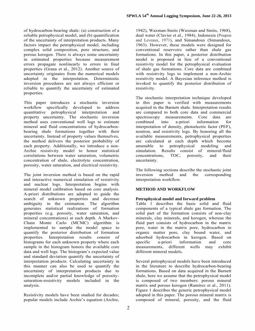
Table 1 describes the basic solid and fluid components of a typical shale gas formation. The solid part of the formation consists of non-clay minerals, clay minerals, and kerogen, whereas the fluid part consists of hydrocarbon in the matrix pore, water in the matrix pore, hydrocarbon in organic matter pore, clay bound water, and adsorbed hydrocarbon in kerogen. Based on specific a-priori information and core measurements, different wells may exhibit different mineral models. Several petrophysical models have been introduced in the literature to describe hydrocarbon-bearing formations. Based on data acquired in the Barnett shale, here we assume that the petrophysical model is composed of two members: porous mineral matrix and porous kerogen (Ramírez et al., 2011). Figure 1 describes the generic petrophysical model adopted in this paper. The porous mineral matrix is composed of mineral, porosity, and the fluid

SPWLA 54th


3

system within the porosity. Porous kerogen includes gas-filled porosity. It is also assumed that kerogen is oil-wet and does not contain water (Wang and Reed, 2009).

Table 1: Basic solid and fluid components of a typical shale gas formation.

Solid Fluid

Illite Water in matrix Chlorite Clay bound water Quartz Hydrocarbon in matrix Feldspars Hydrocarbon in kerogen Dolomite Calcite Pyrite Kerogen

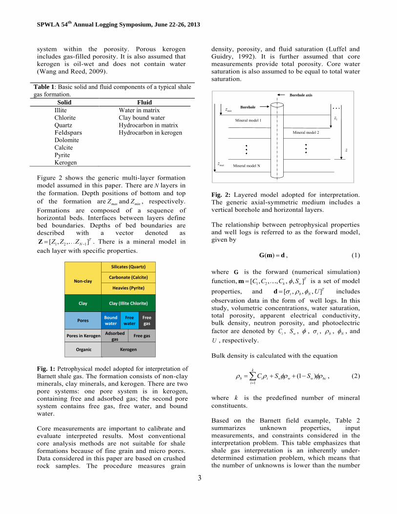
Figure 2 shows the generic multi-layer formation model assumed in this paper. There are N layers in the formation. Depth positions of bottom and top of the formation are maxZ and minZ , respectively. Formations are composed of a sequence of horizontal beds. Interfaces between layers define bed boundaries. Depths of bed boundaries are described with a vector denoted as

1 2 1[ , , ]TNZ Z Z Z . There is a mineral model in

each layer with specific properties.

Fig. 1: Petrophysical model adopted for interpretation of Barnett shale gas. The formation consists of non-clay minerals, clay minerals, and kerogen. There are two pore systems: one pore system is in kerogen, containing free and adsorbed gas; the second pore system contains free gas, free water, and bound water. Core measurements are important to calibrate and evaluate interpreted results. Most conventional core analysis methods are not suitable for shale formations because of fine grain and micro pores. Data considered in this paper are based on crushed rock samples. The procedure measures grain

density, porosity, and fluid saturation (Luffel and Guidry, 1992). It is further assumed that core measurements provide total porosity. Core water saturation is also assumed to be equal to total water saturation.

Fig. 2: Layered model adopted for interpretation. The generic axial-symmetric medium includes a vertical borehole and horizontal layers. The relationship between petrophysical properties and well logs is referred to as the forward model, given by

( ) G m d , (1)

where G is the forward (numerical simulation) function, 1 2[ , , , , , ]T

k wC C C Sm is a set of model properties, and [ , , , ]T

t b N U d includes observation data in the form of well logs. In this study, volumetric concentrations, water saturation, total porosity, apparent electrical conductivity, bulk density, neutron porosity, and photoelectric factor are denoted by iC , wS , , t , b , N , and U , respectively. Bulk density is calculated with the equation

1(1 )

k

b i i w w w hci

C S S

, (2)

where k is the predefined number of mineral constituents. Based on the Barnett field example, Table 2 summarizes unknown properties, input measurements, and constraints considered in the interpretation problem. This table emphasizes that shale gas interpretation is an inherently under-determined estimation problem, which means that the number of unknowns is lower than the number

Organic

Pores in Kerogen

Silicates (Quartz)

Carbonate (Calcite)

Heavies (Pyrite)

Clay (Illite Chlorite)

Kerogen

Free gas

Free water

Boundwater

Non-clay

Clay

Pores

Adsorbed gas

Free gas

Mineral model 2

Mineral model 1

Mineral model N

Borehole axis

Boreholeminz

1z

1Nz

maxz

SPWLA 54th


4

of input measurements and constraints. To circumvent this difficulty, we implement a statistical constraint between different minerals and their concentrations to reduce the number of unknown mineral concentrations.

Table 2: Summary of unknown and inputs properties for the Barnett shale, together with constraints adopted to estimate properties.

Unknowns Input

Porosity Photoelectric factor Water saturation Bulk density Calcite Neutron porosity Quartz/feldspars Electrical resistivity Illite Chlorite Kerogen Pyrite Hydrocarbon

Mass balance equation Kerogen and pyrite constraint Illite and chlorite constraint

We simulate PEF, density, and neutron logs using the fast linear iterative refinement method developed by Mendoza et al. (2010), that explicitly incorporates borehole and formation environmental conditions. Schlumberger’s SNUPAR code (McKeon and Scott, 1989) is used to calculate migration length and photoelectric factor from formation properties. Table 3 summarizes the mineral compositions and chemical formulas adopted for interpretation of the Barnett shale gas formation. A resistivity model is required to estimate water saturation. The challenge is, however, that common deterministic models are often not suitable for shale gas interpretation. Instead, we introduce a Bayesian inference method to quantify a posterior model for electrical resistivity.

Table 3: Mineral model adopted for the Barnett shale gas reservoir.

Component Chemical Formula

Quartz SiO2 Calcite CaCO3 Illite K0.8Al1.6Fe0.2Mg0.2Si3.4Al0.6O10(OH)2 Chlorite Mg5AlSi3AlO10(OH)8 Pyrite Kerogen Water Hydrocarbon/Gas

FeS2 C40H51O3S2N H2O CH4

Stochastic method and Bayesian rule

To perform interpretation of shale gas formations one needs to estimate vector m from the available well logs. In the Barnett field case, measurements consist of noisy density, neutron, resistivity, and PEF logs. We denote the a-priori distribution of

formation properties as ( )p m , the likelihood function as ( | )p d m , and the posterior probability distribution for properties as ( | )q m d . A-priori information aids in determining unknown properties and mitigates non-uniqueness in the interpretation, especially in under-determined estimation problems. The posterior distribution quantifies how well a formation model agrees with prior information and available measurements. Bayes’ theorem relates a-priori and posterior distributions in a way that makes the computations of ( | )q m d tractable (Aster et al., 2005). It can be written as

( | ) ( )( | )( )

p pqp

d m m

m dd

. (3)

Because d contains the data set which includes different well logs, ( )p d is a marginal likelihood and is not a function of model m . Thus, ( )p d will be absorbed as a constant, whereby equation 3 becomes

( | ) ( | ) ( )q p pm d d m m . (4)

A-priori models

The prior distribution of parameters is determined from prior petrophysical knowledge or other external and independent information about unknown properties. In general, the a-priori model is a multidimensional probability distribution (Buland and Kolbjørnsen, 2012). It is assumed that properties in different layers are stochastically independent in the a-priori model. To minimize subjectivity in shale gas interpretation, three rules are imposed to obtain a-priori information. First, we assume in this study that mineral volumetric concentrations follow uniform distributions. The probability density function (PDF) of the continuous uniform distribution is written as

1( )

0

ii

i i

for a C bf C b a

for C a or C b

, (5)

where iC denotes the unknown volumetric concentrations. In general, 0a and 1b . For specific cases, one may gather a-priori information from core measurements. Parameter a and b are set according to stochastic results ascertained from core measurements. The second type of a-priori

SPWLA 54th


5

information is a normal distribution. Specifically, we assume that porosity and water saturation follow a normal distribution. Without loss of generality, the expected value is set based on core measurements. We define the a-priori distribution as

11( ) exp ( ) ( )2

Tprior priorp

mm m m C m m , (6)

where priorm is the prior expected value of

petrophysical properties and m

C is a covariance matrix incorporating the standard deviation of unknown properties. The third type of a-priori information is an uninformative prior (Carlin and Louis, 1996). This a-priori information is employed in the analysis when core measurements or prior field knowledge are not available. Likelihood function

The likelihood function measures the probability of observing the data, d , when the model is m . We denote the likelihood function as ( | )p d m and calculate it by forward modeling ( )G m and assessing the mismatch between measurements and their simulations. According to physical experience, we assume the noise of resistivity measurements to be represented by a lognormal distribution, whereas density, neutron, and PEF exhibit normally distributed noise. For resistivity measurements, one has

1

( | )1exp ln( ( )) ln( ) ln( ( )) ln( ) ,2

r

Tr D r

p

d m

G m d C G m d (7)

where DC is the covariance matrix for the logarithm of the data, rd . Let dC be the covariance matrix for density, neutron, and PEF measurements; we have

1

( | )1exp ( ) ( )2

d

Td d d

p

d m

G m d C G m d (8)

where dd includes density, neutron, and PEF measurements. A data weighting matrix, W , is set to quantify the relative importance and reliability of different measurements during the inversion. For example, when the target properties are mineral concentrations, matrix W emphasizes (higher

weight) the density and PEF measurements. On the other hand, when the target property is water saturation, the data weighting matrix emphasizes the resistivity measurements. Thus, the likelihood functions become

1

( | )1exp ln( ( )) ln( ) ln( ( )) ln( )2

r

T Tr D r

p

d m

G m d W C W G m d

and

1

( | )1exp ( ) ( ) .2

d

T Td d d

p

d m

G m d W C W G m d (9)

Non-Archie resistivity model

For the shale gas resistivity model, the relationship between apparent resistivity measurements and petrophysical properties is not clear. The physical meaning of Archie’s parameters ( a , m , n , and water resistivity) is not fully understood in practice. We examined Archie’s equation with Barnet field data using 1a , 2m , and 2n . To match simulated resistivity logs with original resistivity logs, water resistivity must be set to an extremely low value, which is too low to be physically plausible. Alternative resistivity models were also tested, including Indonesia, dual water, and Simandoux, encountering similar unrealistic values of water resistivity. To circumvent this problem, here we introduce a Bayesian inference method to quantify a posterior distribution for the resistivity model. To that end, we assume that the model can be expressed as

( , , ,1/ ,1/ , )w sh w sh shR f S C R R , (10)

where shC , shR , sh , and R are volumetric concentration, resistivity, shale porosity, and apparent resistivity, respectively. The rule for our method is given by

( | , , ,1/ ,1/ , )( , , ,1/ ,1/ , | ) ( )

( , , ,1/ ,1/ , )

w sh w sh sh

w sh w sh sh

w sh w sh sh

q R S C R Rp S C R R R p R

p S C R R

, (11)

where ( )p is the a-priori PDF, ( )q is the posterior PDF, and ( | ) p is the likelihood function. To avoid specific assumptions about parameter distributions, an uninformative prior is adopted as PDF of the unknown formation properties. Thus a-priori distributions of 1/ wR ,1/ shR , and sh become constants. The a-priori PDF of resistivity is calculated from well logs, whereas the likelihood

SPWLA 54th


6

functions ( | )wp S R , ( | )p R , and ( | )shp C R are postulated from core measurements. We separate the elements of apparent resistivity into several equally-spaced (in the resistivity domain) entries. Calculated histograms describe the probability of occurrence of a given property value within the prescribed range. The resistivity posterior distribution is defined by Bayes’ theorem, i.e.

( | , , )( | ) ( ) ( | ) ( ) ( | ) ( ).

w sh

w sh

q R S Cp S R p R p R p R p C R p R

(12)

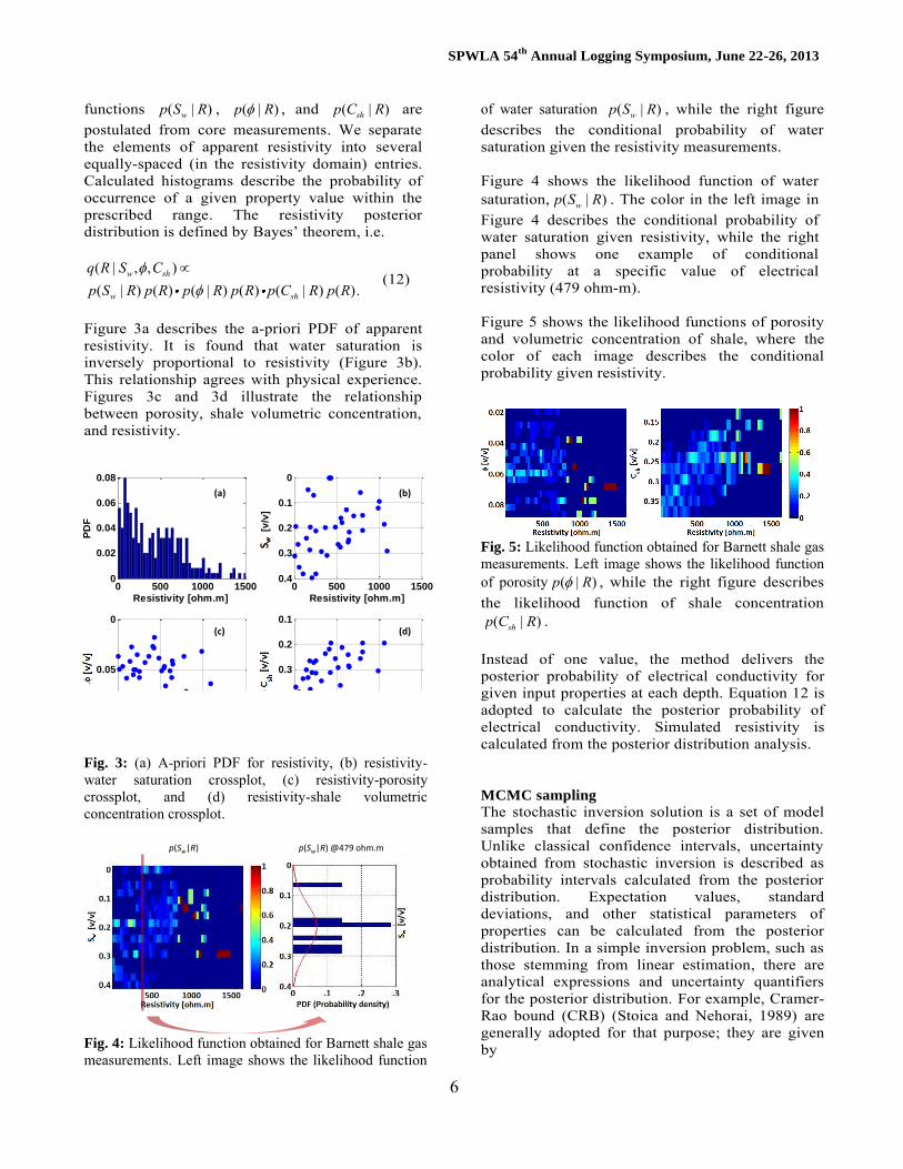
Figure 3a describes the a-priori PDF of apparent resistivity. It is found that water saturation is inversely proportional to resistivity (Figure 3b). This relationship agrees with physical experience. Figures 3c and 3d illustrate the relationship between porosity, shale volumetric concentration, and resistivity.

Fig. 3: (a) A-priori PDF for resistivity, (b) resistivity-water saturation crossplot, (c) resistivity-porosity crossplot, and (d) resistivity-shale volumetric concentration crossplot.

Fig. 4: Likelihood function obtained for Barnett shale gas measurements. Left image shows the likelihood function

of water saturation ( | )wp S R , while the right figure describes the conditional probability of water saturation given the resistivity measurements. Figure 4 shows the likelihood function of water saturation, ( | )wp S R . The color in the left image in Figure 4 describes the conditional probability of water saturation given resistivity, while the right panel shows one example of conditional probability at a specific value of electrical resistivity (479 ohm-m). Figure 5 shows the likelihood functions of porosity and volumetric concentration of shale, where the color of each image describes the conditional probability given resistivity.

Fig. 5: Likelihood function obtained for Barnett shale gas measurements. Left image shows the likelihood function of porosity ( | )p R , while the right figure describes the likelihood function of shale concentration

( | )shp C R . Instead of one value, the method delivers the posterior probability of electrical conductivity for given input properties at each depth. Equation 12 is adopted to calculate the posterior probability of electrical conductivity. Simulated resistivity is calculated from the posterior distribution analysis. MCMC sampling

The stochastic inversion solution is a set of model samples that define the posterior distribution. Unlike classical confidence intervals, uncertainty obtained from stochastic inversion is described as probability intervals calculated from the posterior distribution. Expectation values, standard deviations, and other statistical parameters of properties can be calculated from the posterior distribution. In a simple inversion problem, such as those stemming from linear estimation, there are analytical expressions and uncertainty quantifiers for the posterior distribution. For example, Cramer-Rao bound (CRB) (Stoica and Nehorai, 1989) are generally adopted for that purpose; they are given by

0 500 1000 15000

0.02

0.04

0.06

0.08

Resistivity [ohm.m]

PD

F

0 500 1000 1500

0

0.1

0.2

0.3

0.4

Resistivity [ohm.m]

Sw

[v

/v]

0 500 1000 1500

0

0.05

0.1

Resistivity [ohm.m]

[

v/v

]

0 500 1000 1500

0.1

0.2

0.3

0.4

0.5

Resistivity [ohm.m]

Csh

[v

/v]

(b)(a)

(c) (d)

p(Sw|R) @479 ohm.mp(Sw|R)

SPWLA 54th


7

2* 1

2cov( ) { ln[ ( | )]}E p

m d m

m, (13)

where the uncertainty of the inverted properties is quantified by the estimator’s covariance matrix (Habashy and Abubakar, 2004), written as

* 1 * 1 * 1cov( ) [cov( ) ( ) ( )]dC m m J m J m , (14)

where is the regularization parameter. Equation 14 is the theoretical minimum bound for uncertainty. The necessary and sufficient condition behind equation 14 (Zhang, 2002) is

*ln ( | ) ( )( )p K

d m m m m

m, (15)

where ( )K m is a function of m which has no relationship with d . The interpretation of hydrocarbon-bearing shale from well logs constitutes a nonlinear estimation problem with a non-Gaussian distribution. Equation 15 is a strong assumption about measurement uncertainty which cannot be satisfied in shale interpretation problems. Compared to existing uncertainty analysis methods, MCMC is a reliable and efficient choice to quantify the posterior distribution and perform uncertainty analysis. Alternative solutions to nonlinear estimation problems involve using asymptotic methods to obtain analytical approximations of the posterior density function. The normal approximation and Laplace’s method (Tierney and Kadane, 1986) fall into this category. The idea behind MCMC is to generate random samples from a specified probability distribution by constructing a Markov chain (Buland and Kolbjørnsen, 2012; Gilks et al., 1996), where the specified probability distribution is the posterior distribution in our application. On the other hand, MCMC is independent of the search point, whereby the posterior distribution has no relationship to the initial search point in model space. After an initial ‘burn-in’ period, in which random selections move toward the high posterior probability region, the Markov chain samples a desired posterior distribution. Gibbs sampling (Gelfand and Smith, 1990) and Metropolis-Hastings’s (Metropolis et al., 1953; Hasting, 1970) rule are adopted to trace the Markov chain.

As previously emphasized, unknown properties in the estimation problem are a set of model properties 1 2[ , , , , , ]T

k wC C C Sm , while inputs to the estimation are well logs, [ , , , ]T

t b N U d . The stochastic inversion will deliver the posterior distribution of all the unknown parameters. Let i

m denote the current state of the Markov chain in the i -th iteration. We define

1 2[ , , , , , ]i i i i i i Tk wC C C Sm , (16)

in which max1 i I , with maxI equal to the maximum number of iteration steps. In the first step of inversion, a classical method is adopted to calculate the initial points for each property in i

m (1i ). The posterior distribution for each property

is initial-guess independent; however, a good initial guess can increase the efficiency of the estimation. If we assume that samples, i

m , have been taken from the solution of the estimation problem, then the 1i

m sample of the solution is constructed as follows: any property of 1i

m , for example 1ijm , is

updated from the same property in im , such as i

jm .

Based on ijm , the candidate ,i propose

jm is calculated

from a jumping distribution ,( , )i i proposej jq m m , which

is the probability of returning a value of ,i proposejm

given a previous value of ijm . These are the steps

followed to obtain a random walk chain. In this paper, we employ the volumetric concentration of kerogen, denoted i

kerC , to illustrate in detail the mechanics of the method. Using a jumping distribution to obtain ,i propose

kerC , one has

,i propose iker kerC C , (17)

where is a random variable. Thus,

, ,( , ) ( , ) ( )i i propose i i proposej j ker kerq m m q C C q , (18)

where the jumping distribution is associated with the random variable . In this case, the symmetric normal distribution with zero expected value is adopted to generate the proposed parameters. Consequently,

, ,2, , , , ,

Ti propose i propose i i i iker k wC C C S m . (19)

SPWLA 54th


8

The random proposal function may generate properties that do not make physical sense, for example, a negative volumetric concentration. We solve this problem by setting the acceptance probability to zero in the a-priori distribution for an illegal property candidate. Let

1/ ( ), ,

,

( | ) ( , )( | ) ( , )

ii propose i i proposej j

i i propose ij j

p q m mL

p q m m

T

d m

d m, (20)

where function T is referred to as the cooling schedule, it is a function of iteration step, i . A more detailed introduction to the cooling schedule can be found in Walsh (2004). The function T is adopted to avoid locking into a local optimal peak. The new candidate is accepted with an acceptance probability, which is the rule to accept the ,

keri proposeC .

The rule is given by

,1

1(0,1)i propose

i keriker

C accept when L randm

C reject others

,(21)

where (0,1)rand is a uniform random distribution number. If the new candidate increases the PDF ( 1L ), then it is accepted. If the new candidate decreases the PDF ( 1L ), it is accepted with probability (0,1)rand . Otherwise, the new candidate is rejected and the procedure returns to obtain a new candidate ,i propose

kerC via equation 17. In this manner, the sampling process considers all the properties in the unknown set i

m . When all the parameters in the set i

m are updated, one reaches a new accepted set 1i

m . Following the afore-described procedure, we obtain enough model realizations to quantify the posterior distribution. Yang and Torres-Verdín (2011) introduced a solution to determine the number of steps required to converge to the stationary distribution within an acceptable error. The procedure comes to a halt when any of the following two convergence criteria are satisfied in the iteration process:

(1) The actual iteration number reaches the maximal iteration number, maxI , and

(2) The accepted sample sequence is tested by a modified z-test. Results reach the Geweke z-score requirement (Geweke, 1991).

FIELD CASE

We undertake the interpretation of field data

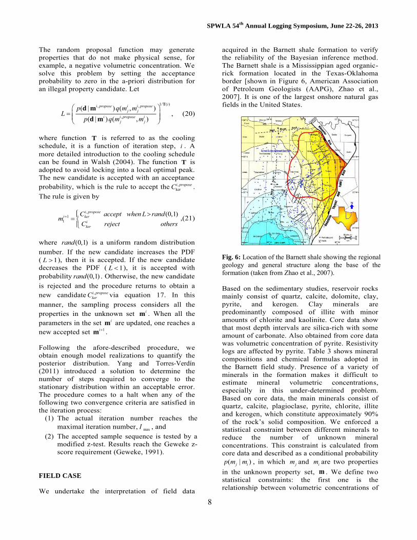
acquired in the Barnett shale formation to verify the reliability of the Bayesian inference method. The Barnett shale is a Mississippian aged organic-rick formation located in the Texas-Oklahoma border [shown in Figure 6, American Association of Petroleum Geologists (AAPG), Zhao et al., 2007]. It is one of the largest onshore natural gas fields in the United States.

Fig. 6: Location of the Barnett shale showing the regional geology and general structure along the base of the formation (taken from Zhao et al., 2007). Based on the sedimentary studies, reservoir rocks mainly consist of quartz, calcite, dolomite, clay, pyrite, and kerogen. Clay minerals are predominantly composed of illite with minor amounts of chlorite and kaolinite. Core data show that most depth intervals are silica-rich with some amount of carbonate. Also obtained from core data was volumetric concentration of pyrite. Resistivity logs are affected by pyrite. Table 3 shows mineral compositions and chemical formulas adopted in the Barnett field study. Presence of a variety of minerals in the formation makes it difficult to estimate mineral volumetric concentrations, especially in this under-determined problem. Based on core data, the main minerals consist of quartz, calcite, plagioclase, pyrite, chlorite, illite and kerogen, which constitute approximately 90% of the rock’s solid composition. We enforced a statistical constraint between different minerals to reduce the number of unknown mineral concentrations. This constraint is calculated from core data and described as a conditional probability

( | )j ip m m , in which jm and im are two properties in the unknown property set, m . We define two statistical constraints: the first one is the relationship between volumetric concentrations of

SPWLA 54th


9

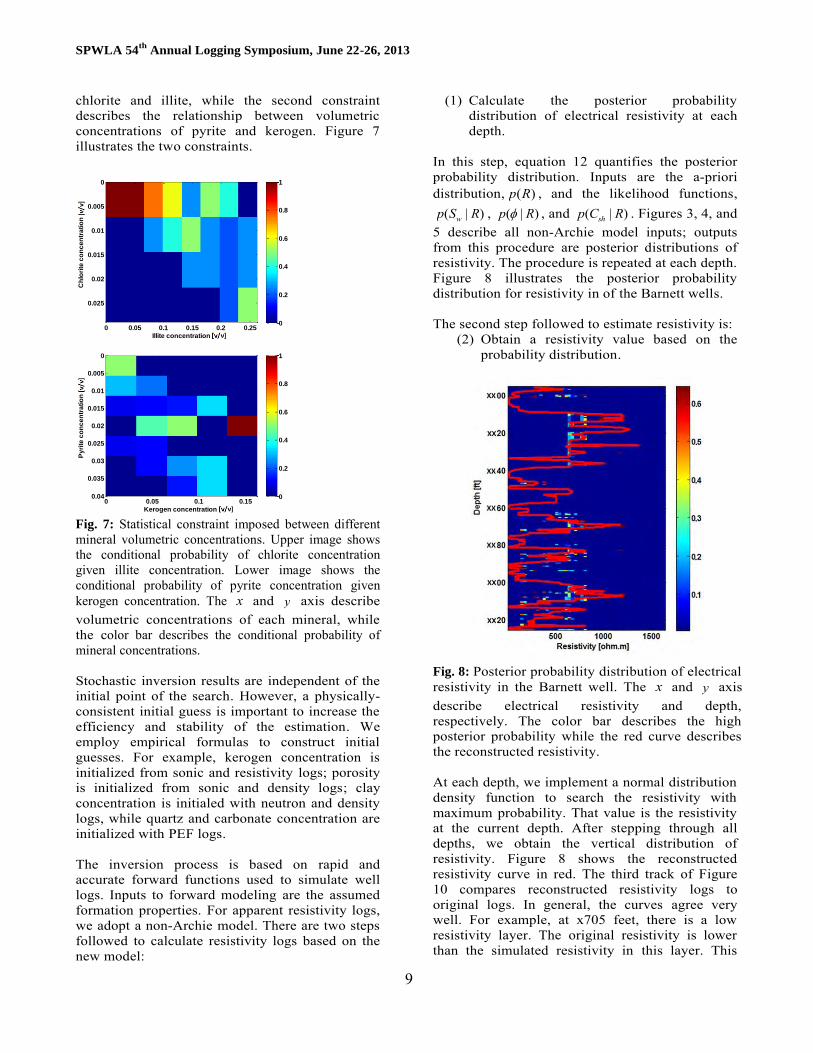
chlorite and illite, while the second constraint describes the relationship between volumetric concentrations of pyrite and kerogen. Figure 7 illustrates the two constraints.

Fig. 7: Statistical constraint imposed between different mineral volumetric concentrations. Upper image shows the conditional probability of chlorite concentration given illite concentration. Lower image shows the conditional probability of pyrite concentration given kerogen concentration. The x and y axis describe volumetric concentrations of each mineral, while the color bar describes the conditional probability of mineral concentrations. Stochastic inversion results are independent of the initial point of the search. However, a physically-consistent initial guess is important to increase the efficiency and stability of the estimation. We employ empirical formulas to construct initial guesses. For example, kerogen concentration is initialized from sonic and resistivity logs; porosity is initialized from sonic and density logs; clay concentration is initialed with neutron and density logs, while quartz and carbonate concentration are initialized with PEF logs. The inversion process is based on rapid and accurate forward functions used to simulate well logs. Inputs to forward modeling are the assumed formation properties. For apparent resistivity logs, we adopt a non-Archie model. There are two steps followed to calculate resistivity logs based on the new model:

(1) Calculate the posterior probability distribution of electrical resistivity at each depth.

In this step, equation 12 quantifies the posterior probability distribution. Inputs are the a-priori distribution, ( )p R , and the likelihood functions,

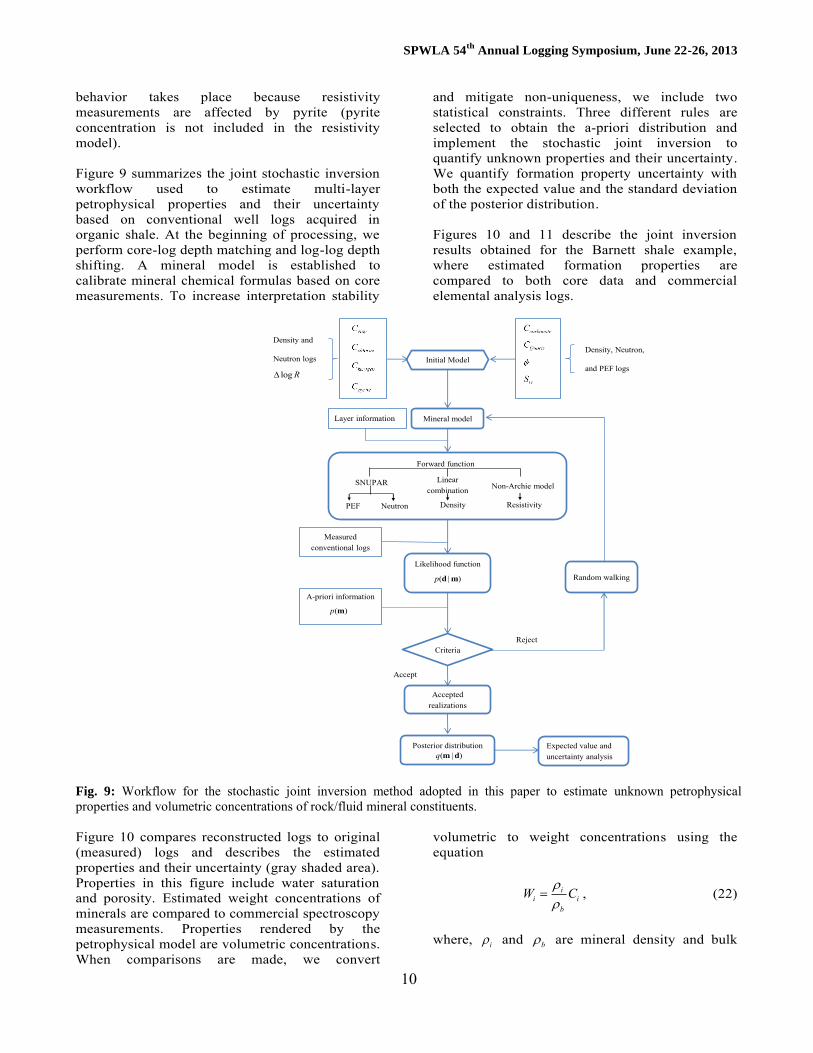
( | )wp S R , ( | )p R , and ( | )shp C R . Figures 3, 4, and 5 describe all non-Archie model inputs; outputs from this procedure are posterior distributions of resistivity. The procedure is repeated at each depth. Figure 8 illustrates the posterior probability distribution for resistivity in of the Barnett wells. The second step followed to estimate resistivity is:

(2) Obtain a resistivity value based on the probability distribution.

Fig. 8: Posterior probability distribution of electrical resistivity in the Barnett well. The x and y axis describe electrical resistivity and depth, respectively. The color bar describes the high posterior probability while the red curve describes the reconstructed resistivity. At each depth, we implement a normal distribution density function to search the resistivity with maximum probability. That value is the resistivity at the current depth. After stepping through all depths, we obtain the vertical distribution of resistivity. Figure 8 shows the reconstructed resistivity curve in red. The third track of Figure 10 compares reconstructed resistivity logs to original logs. In general, the curves agree very well. For example, at x705 feet, there is a low resistivity layer. The original resistivity is lower than the simulated resistivity in this layer. This

Illite concentration

Ch

lori

te c

on

ce

ntr

ati

on

0 0.05 0.1 0.15 0.2 0.25

0

0.005

0.01

0.015

0.02

0.025

0

0.2

0.4

0.6

0.8

1

Kerogen concentration

Py

rite

co

nc

en

tra

tio

n

0 0.05 0.1 0.15

0

0.005

0.01

0.015

0.02

0.025

0.03

0.035

0.04 0

0.2

0.4

0.6

0.8

1

SPWLA 54th


10

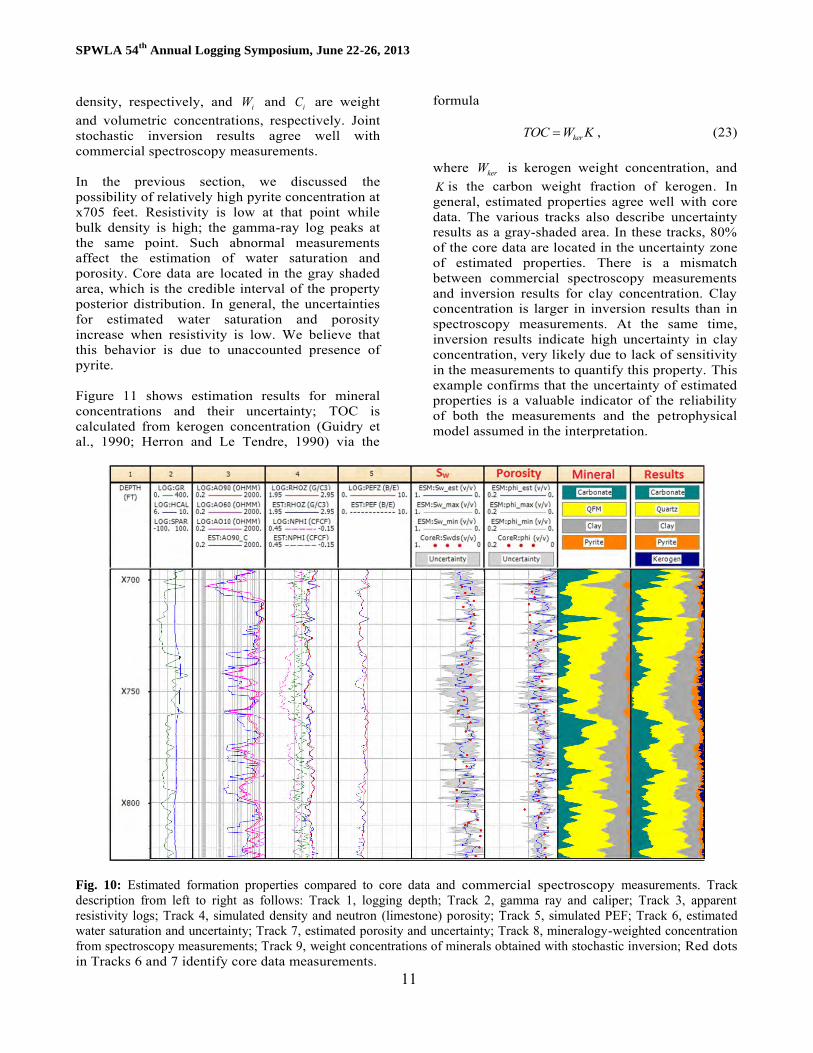
behavior takes place because resistivity measurements are affected by pyrite (pyrite concentration is not included in the resistivity model). Figure 9 summarizes the joint stochastic inversion workflow used to estimate multi-layer petrophysical properties and their uncertainty based on conventional well logs acquired in organic shale. At the beginning of processing, we perform core-log depth matching and log-log depth shifting. A mineral model is established to calibrate mineral chemical formulas based on core measurements. To increase interpretation stability

and mitigate non-uniqueness, we include two statistical constraints. Three different rules are selected to obtain the a-priori distribution and implement the stochastic joint inversion to quantify unknown properties and their uncertainty. We quantify formation property uncertainty with both the expected value and the standard deviation of the posterior distribution. Figures 10 and 11 describe the joint inversion results obtained for the Barnett shale example, where estimated formation properties are compared to both core data and commercial elemental analysis logs.

Fig. 9: Workflow for the stochastic joint inversion method adopted in this paper to estimate unknown petrophysical properties and volumetric concentrations of rock/fluid mineral constituents. Figure 10 compares reconstructed logs to original (measured) logs and describes the estimated properties and their uncertainty (gray shaded area). Properties in this figure include water saturation and porosity. Estimated weight concentrations of minerals are compared to commercial spectroscopy measurements. Properties rendered by the petrophysical model are volumetric concentrations. When comparisons are made, we convert

volumetric to weight concentrations using the equation

ii i

b

W C

, (22)

where, i and b are mineral density and bulk

Initial Model

Mineral model

Density and

Neutron logsDensity, Neutron,

and PEF logs

Layer information

Forward function

PEF Neutron Density Resistivity

SNUPAR Linear combination Non-Archie model

Likelihood function

Measured conventional logs

A-priori information

Criteria

Accepted realizations

Posterior distribution Expected value and uncertainty analysis

Accept

Random walking

Reject

log R

( | )p d m

( )p m

( | )q m d

SPWLA 54th


11

density, respectively, and iW and iC are weight and volumetric concentrations, respectively. Joint stochastic inversion results agree well with commercial spectroscopy measurements. In the previous section, we discussed the possibility of relatively high pyrite concentration at x705 feet. Resistivity is low at that point while bulk density is high; the gamma-ray log peaks at the same point. Such abnormal measurements affect the estimation of water saturation and porosity. Core data are located in the gray shaded area, which is the credible interval of the property posterior distribution. In general, the uncertainties for estimated water saturation and porosity increase when resistivity is low. We believe that this behavior is due to unaccounted presence of pyrite. Figure 11 shows estimation results for mineral concentrations and their uncertainty; TOC is calculated from kerogen concentration (Guidry et al., 1990; Herron and Le Tendre, 1990) via the

formula

kerTOC W K , (23)

where kerW is kerogen weight concentration, and K is the carbon weight fraction of kerogen. In general, estimated properties agree well with core data. The various tracks also describe uncertainty results as a gray-shaded area. In these tracks, 80% of the core data are located in the uncertainty zone of estimated properties. There is a mismatch between commercial spectroscopy measurements and inversion results for clay concentration. Clay concentration is larger in inversion results than in spectroscopy measurements. At the same time, inversion results indicate high uncertainty in clay concentration, very likely due to lack of sensitivity in the measurements to quantify this property. This example confirms that the uncertainty of estimated properties is a valuable indicator of the reliability of both the measurements and the petrophysical model assumed in the interpretation.

Fig. 10: Estimated formation properties compared to core data and commercial spectroscopy measurements. Track description from left to right as follows: Track 1, logging depth; Track 2, gamma ray and caliper; Track 3, apparent resistivity logs; Track 4, simulated density and neutron (limestone) porosity; Track 5, simulated PEF; Track 6, estimated water saturation and uncertainty; Track 7, estimated porosity and uncertainty; Track 8, mineralogy-weighted concentration from spectroscopy measurements; Track 9, weight concentrations of minerals obtained with stochastic inversion; Red dots in Tracks 6 and 7 identify core data measurements.

SPWLA 54th


12

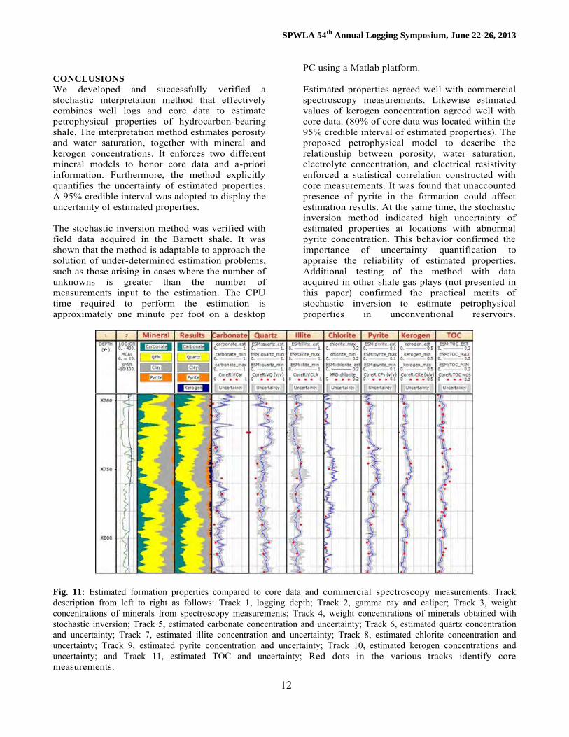
CONCLUSIONS

We developed and successfully verified a stochastic interpretation method that effectively combines well logs and core data to estimate petrophysical properties of hydrocarbon-bearing shale. The interpretation method estimates porosity and water saturation, together with mineral and kerogen concentrations. It enforces two different mineral models to honor core data and a-priori information. Furthermore, the method explicitly quantifies the uncertainty of estimated properties. A 95% credible interval was adopted to display the uncertainty of estimated properties. The stochastic inversion method was verified with field data acquired in the Barnett shale. It was shown that the method is adaptable to approach the solution of under-determined estimation problems, such as those arising in cases where the number of unknowns is greater than the number of measurements input to the estimation. The CPU time required to perform the estimation is approximately one minute per foot on a desktop

PC using a Matlab platform. Estimated properties agreed well with commercial spectroscopy measurements. Likewise estimated values of kerogen concentration agreed well with core data. (80% of core data was located within the 95% credible interval of estimated properties). The proposed petrophysical model to describe the relationship between porosity, water saturation, electrolyte concentration, and electrical resistivity enforced a statistical correlation constructed with core measurements. It was found that unaccounted presence of pyrite in the formation could affect estimation results. At the same time, the stochastic inversion method indicated high uncertainty of estimated properties at locations with abnormal pyrite concentration. This behavior confirmed the importance of uncertainty quantification to appraise the reliability of estimated properties. Additional testing of the method with data acquired in other shale gas plays (not presented in this paper) confirmed the practical merits of stochastic inversion to estimate petrophysical properties in unconventional reservoirs.

Fig. 11: Estimated formation properties compared to core data and commercial spectroscopy measurements. Track description from left to right as follows: Track 1, logging depth; Track 2, gamma ray and caliper; Track 3, weight concentrations of minerals from spectroscopy measurements; Track 4, weight concentrations of minerals obtained with stochastic inversion; Track 5, estimated carbonate concentration and uncertainty; Track 6, estimated quartz concentration and uncertainty; Track 7, estimated illite concentration and uncertainty; Track 8, estimated chlorite concentration and uncertainty; Track 9, estimated pyrite concentration and uncertainty; Track 10, estimated kerogen concentrations and uncertainty; and Track 11, estimated TOC and uncertainty; Red dots in the various tracks identify core measurements.

SPWLA 54th


13

ACKNOWLEDGEMENTS

The work reported in this paper was funded by The University of Texas at Austin's Research Consortium on Formation Evaluation, jointly sponsored by Afren, Anadarko, Apache, Aramco, Baker-Hughes, BG, BHP Billiton, BP, Chevron, China Oilfield Services, LTD., ConocoPhillips, ENI, ExxonMobil, Halliburton, Hess, Maersk, Marathon Oil Corporation, Mexican Institute for Petroleum, Nexen, ONGC, OXY, Petrobras, Repsol, RWE, Schlumberger, Shell, Statoil, Total, Weatherford, Wintershall, and Woodside Petroleum Limited.

SYMBOLS

mC : Covariance matrix of unknown properties.

DC : Covariance matrix for the logarithm of the measurements.

dC : Covariance matrix for the measurements.

iC : Volumetric concentration. d : Measurement vector.

maxI : Maximum number of iteration steps. k : Predefined number of mineral constituents. L : Ratio of likelihood function. m : Model parameter vector.

priorm : A-priori expected value of properties. i

m : Model parameter vector in the i -th steps of the inversion.

*m : Model parameter solution.

ijm : j -th parameter in the i -th steps of the

inversion. ,i proposejm : Candidate j -th parameter of model in the

i -th steps of the inversion. N : Number of layers.

t : Apparent conductivity. : Porosity.

b : Bulk density.

N : Neutron porosity. : Random offset. R : Apparent resistivity.

wS : Water saturation. T : Cooling schedule of the simulated

annealing method. T : Transpose of a matrix. : Regularization parameter. U : Photoelectric factor. W : Weighting matrix.

minZ : Minimal boundary of layered model.

maxZ : Maximal boundary of layered model.

Z : Bed-boundary vector. cov( ) : Covariance matrix function.

( )E : Expected value function. ( )G : Forward function.

( )J : Jacobian matrix function. ( )p m : A-priori distribution of model parameters. ( )p d : Marginal likelihood of measurements. ( | )p d m : Conditional probability distribution. ( | )q m d : Posterior probability distribution for

model parameters. ( | )w tp S R : Likelihood function of water saturation. ( | )tp R : Likelihood function of porosity. ( | )sh tp C R :Likelihood function of shale

concentration. ( | )j ip m m : Conditional probability between two

properties. (0,1)rand : Uniform distribution.

ACRONYMS

AAPG: American Association of Petroleum Geologists.

CRB: Cramer-Rao bounds. MCMC: Markov-Chain Monte Carlo. PDF: Probability density function. PEF: Photoelectric factor. TOC: Total organic carbon.

REFERENCES

Archie, G. E., 1942, The electrical resistivity log as an aid in determining some reservoir characteristics: Petroleum Transactions, AIME, vol. 146, pp. 54-62.

Aster, R. C., Borchers, B., and Thurber, C. H., 2005, Parameter Estimation and Inverse Problems: Elsevier Academic.

Buland, A., and Kolbjørnsen, O., 2012, Bayesian inversion of CSEM and magnetotelluric data: Geophysics, vol. 77, no. 1, pp. E33-E42.

Carlin, P. B. and Louis, A. T., 1996, Bayes and Empirical Bayes Methods for Data Analysis: Chapman and Hall.

Clavier, C. and Rust, D.H., 1976, MID-plot: A new lithology technique: The Log Analyst, vol. 17, no. 6.

Clavier, C., Coates, G., and Dumanoir, J., 1984, Theoretical and experimental bases for the dual-water model for interpretation of shaly sands: SPE Journal, vol. 24, pp. 153-167.

Darling, T., 2005, Well Logging and Formation Evaluation: Gulf Professional Publishing.

Ellis, D. V. and Singer, J. M., 2007, Well Logging for Earth Scientists: Springer.

Gelfand, A. E. and Smith, A. F. M., 1990, Sampling-based approached to calculation marginal densities:

SPWLA 54th


14

Journal of the American Statistical Association, vol. 85, no. 410, pp. 398-409.

Geweke, J., 1991, Evaluating the accuracy of sampling-based approaches to the calculation of posterior moments: Federal Reserve Bank of Minneapolis, Research Department Staff Report 148.

Gilks, W. R., Richardson, S., and Spiegelhalter, D., 1995, Markov Chain Monte Carlo in Practice: Chapman & Hall/CRC.

Grana, D., Pirrone, M., and Mukerji, T., 2012, Quantitative log interpretation and uncertainty propagation of petrophysical properties and facies classification from rock-physics modeling and formation evaluation analysis: Geophysics, vol. 77, no. 3, WA45-WA63.

Guidry, F. K., Luffel, D. L., Olszewski, A. J., and Scheper, R. J,. 1996, Devonian shale formation evaluation model based on logs, new core analysis methods, and production tests: SPE reprint series, pp. 101-120.

Habashy, T. M. and Abubakar, A., 2004, A general framework for constraint minimization for the inversion of electromagnetic measurements: Progress in Electromagnetics Research, 46, pp. 265-312.

Hastings, W.K., 1970, Monte Carlo sampling methods using Markov chains and their applications: Biometrika, vol. 57, no. 1, pp. 97-109.

Heidari, Z., Torres-Verdín, C., and W. E. Preeg., 2010, Improved estimation of mineral and fluid volumetric concentrations in thinly-bedded and invaded formations: Transactions of the SPWLA 51st Annual Symposium, Perth, Australia, June 19-23.

Herron, S. L. and Le Tendre, L., 1990, Wireline source-rock evaluation in the Paris basin: AAPG Studies in Geology, vol. 30, no. 57.

Luffel, D. L., and Guidry, F. K., 1992, New core analysis methods for measuring reservoir rock properties of Devonian shale: Journal of Petroleum Technology, vol. 44, no. 11, pp. 1184-1190.

McKeon, D.C. and Scott, H.D., 1989, SNUPAR-a nuclear parameter code for nuclear geophysics applications: IEEE Transactions on Nuclear Science, vol. 36, no. 1, pp. 1215-1219.

Mendoza, A., Torres-Verdín, C., and Preeg, W. E., 2010, Linear iterative refinement method for the rapid simulation of borehole nuclear measurements, part i: vertical wells: Geophysics, vol. 75, no. 1, pp. E9-E29.

Metropolis, N., Rosenbluth, A.W., Rosenbluth, M.N., Teller, A.H., and Teller, E., 1953, Equations of state calculations by fast computing machines: Journal of Chemical Physics, vol. 21, pp. 1087-1091.

Poupon, A. and Leveaux, J., 1971, Evaluation of water saturation in shaly formations: Transactions of SPWLA 12th Annual Logging Symposium, pp. 1-2.

Ramírez, T., Klein, J., Bonnie, R., and Howard, J., 2011, Comparative study of formation evaluation methods for unconventional shale gas reservoirs: application to the Haynesville shale (Texas): North American

Unconventional Gas Conference and Exhibition, SPE 144052.

Simandoux, P., 1963, Dielectric measurements in porous media and application to shaly formation: Revue del’Institut Francais du Petrole, Supplementary Issue, pp.193-215.

Stoica, P. and Nehorai, A., 1989, MUSIC, maximum likelihood, and Cramer-Rao bound: IEEE Transactions on Signal Processing, vol. 3, no. 5, pp. 720-741.

Tierney, L. and Kadane, J. B., 1986, Accurate approximations for posterior moments and marginal densities: Journal of the American Statistical Association, vol. 81, no. 393, pp. 82-86.

Walsh, B., 2004, Markov Chain Monte Carlo and Gibbs Sampling: Lecture Notes for EEB 581, version 26.

Wang, F. and Reed, R., 2009, Pore networks and fluid flow in gas shales: SPE Annual Technical Conference and Exhibition, 124253-MS.

Waxman, M. H. and Smits, L. J. M., l968, Electrical conductivities in oil bearing shaly sands: SPE Journal, vol. 24, pp. 107-122.

Zhang, X., 2002, Modern Signal Processing: Tsinghua University Press.

Yang, Q. and Torres-Verdín, C., 2011, Efficient 2D Bayesian Inversion of borehole resistivity measurements: 82nd SEG Annual Meeting, San Antonio, Texas, USA, September18 – 23, pp. 427-431.

Zhao, H., Givens, N. B., and Curtis, B., 2007, Thermal maturity of the Barnett Shale determined from well-log analysis: AAPG bulletin, vol. 91, no. 4, pp. 535-549.

ABOUT THE AUTHORS

Qinshan Yang is a research fellow with the Department of Petroleum and Geosystems Engineering at The University of Texas at Austin. He has been with the University since 2010. He received his Ph.D. in signal and information processing from the Chinese Academy of Sciences in 2003. His research interests include borehole geophysics, petrophysics, formation evaluation, well logging, integrated reservoir description, signal processing, and inverse problems. From 2006 to 2010, he worked with the China National Petroleum Corporation as Vice Dean for the Logging Research Institute. From 2003 to 2006 he worked for Schlumberger in BGC and IPC.

Carlos Torres-Verdín received a Ph.D. in Engineering Geoscience from the University of California at Berkeley in 1991. During 1991–1997 he held the position of Research Scientist with Schlumberger-Doll Research. From 1997–1999 he was Reservoir Specialist and Technology Champion with YPF (Buenos Aires, Argentina). Since 1999, he has been with the Department

SPWLA 54th


15

of Petroleum and Geosystems Engineering at The University of Texas at Austin, where he is currently holds the Zarrow Centennial Professorship. He conducts research on borehole geophysics, formation evaluation, well logging, and integrated reservoir characterization. Dr. Torres-Verdín is the founder and director of the Joint Industry Research Consortium on Formation Evaluation at The University of Texas at Austin.

JOINT STOCHASTIC INTERPRETATION OF CONVENTIONAL WELL … · JOINT STOCHASTIC INTERPRETATION OF...

Documents

Transcript of JOINT STOCHASTIC INTERPRETATION OF CONVENTIONAL WELL … · JOINT STOCHASTIC INTERPRETATION OF...