C© 2005 Springer Science + Business Media, Inc. Manufactured in The Netherlands.

An Autonomic Reservoir Framework for the Stochastic Optimizationof Well Placement

WOLFGANG BANGERTH and HECTOR KLIECenter for Subsurface Modeling, The University of Texas at Austin, Austin, TX

VINCENT MATOSSIAN and MANISH PARASHARThe Applied Software Systems Laboratory, Rutgers University, Piscataway, NJ

MARY F. WHEELERCenter for Subsurface Modeling, The University of Texas at Austin, Austin, TX

Abstract. The adequate location of wells in oil and environmental applications has a significant economic impact on reservoir management.However, the determination of optimal well locations is both challenging and computationally expensive. The overall goal of this research isto use the emerging Grid infrastructure to realize an autonomic self-optimizing reservoir framework. In this paper, we present a policy-drivenpeer-to-peer Grid middleware substrate to enable the use of the Simultaneous Perturbation Stochastic Approximation (SPSA) optimizationalgorithm, coupled with the Integrated Parallel Accurate Reservoir Simulator (IPARS) and an economic model to find the optimal solutionfor the well placement problem.

Keywords: Grid computing, autonomic Grid middleware, stochastic optimization, optimal well placement, reservoir management

1. Introduction

The locations of wells in oil and environmental applica-tions significantly affect the productivity and environmen-tal/economic benefits of a subsurface reservoir. However, thedetermination of optimal well locations is a challenging prob-lem since it depends on geological and fluid properties as wellas on economic parameters. This leads to a very large numberof potential scenarios that must be evaluated using numeri-cal reservoir simulations. Reservoir simulators are based onthe numerical solution of a complex set of coupled nonlinearpartial differential equations over hundreds of thousands tomillions of gridblocks. The high costs of simulation make anexhaustive evaluation of all these scenarios infeasible. As aresult, the well locations are traditionally determined by an-alyzing only a few scenarios. However, this ad hoc approachmay often lead to incorrect decisions with a high economicimpact.

Optimization algorithms offer the potential for a systematicexploration of a broader set of scenarios to identify optimumlocations under given conditions. These algorithms togetherwith the experienced judgment of specialists, allow a betterassessment of uncertainty and significantly reduce the riskin decision-making. Consequently, there is an increasing in-terest in the use of optimization algorithms for finding theoptimum well location in oil industry [4,8,17,32]. However,the selection of appropriate optimization algorithms, the run-time configuration and invocation of these algorithms, and thedynamic optimization of the reservoir remain a challengingproblem.

The overall goal of this research is to use the emerging Gridinfrastructure [7] and its support for seamless aggregations,compositions and interactions, to realize an autonomic self-optimizing reservoir application. The application consists of:(1) sophisticated reservoir simulation components that encap-sulate complex mathematical models of the physical interac-tion in the subsurface, and execute on distributed computingsystems on the Grid; (2) Grid services that provide secure andcoordinated access to the resources required by the simula-tions; (3) distributed data archives that store historical, ex-perimental and observed data; (4) sensors embedded in theinstrumented oilfield providing real-time data about the cur-rent state of the oil field; (5) external services that provide datarelevant to optimization of oil production or of the economicprofit such as current weather information or current prices;and (6) the actions of scientists, engineers and other experts,in the field, the laboratory, and in management offices.

These components need to dynamically discover one an-other and interact as peers to achieve the overall applica-tion objectives. First, the simulation components interact withGrid services to dynamically obtain necessary resources, de-tect current resource state, and negotiate required quality ofservice. Next, we recall that the data necessary for reservoirsimulation is usually sparse and incomplete; in particular, thisconcerns the data on the geology of the subsurface and onthe resident fluids which are very difficult to obtain. There-fore, the simulation components interact with one anotherand with data archives and real-time sensor data to enablebetter characterization of the reservoir through processes ofdynamic data injection, and data driven adaptations. Then,

Cluster Computing 8, 255–269, 2005

256 BANGERTH ET AL.

the reservoir simulation components interact with other ser-vices on the Grid, for example, with optimization servicesto optimize well placement, with weather services to controlproduction, and with economic modeling services to detectcurrent and predicted future oil prices so as to maximize therevenue from the production. Finally, the experts (scientists,engineers, and managers) collaboratively access, monitor, in-teract with, and steer the simulations and data at runtime todrive the discovery process.

The overall oil production process described above is au-tonomic in that the peers involved automatically detect sub-optimal oil production behaviors at runtime and orchestrateinteractions among themselves to correct this behavior. Fur-ther, the detection and optimization process is achieved usingpolicies and constraints that minimize human intervention.The interactions between instances of peer services are op-portunistic, based on runtime discovery and specified policies,and are not predefined.

In this paper we use our prototype autonomic reservoirframework [15] to investigate the policy-driven runtime selec-tion and invocation of optimization services to determine opti-mal well placement and configuration. The specific objectivesof this paper include: (1) characterization of the behavior andapplicability of optimization techniques for oil reservoir opti-mization; (2) formulation of policies for the runtime selectionand invocation of optimization services for well placement;and (3) the design of a prototype policy-driven frameworkfor autonomic reservoir optimization in Grid environments.In our earlier work [15], we studied the use of the Very FastSimulated Annealing (VFSA) [24] optimization technique.In this paper we use the Simultaneous Perturbation StochasticApproximation (SPSA) [25,27] algorithm for optimizing wellplacement.

The reservoir framework consists of (i) instances of dis-tributed multi-model, multi-block reservoir simulation com-ponents provided by the IPARS reservoir simulator frame-work, (ii) optimization services based on the SPSA algorithm,(iii) economic modeling services, (iv) real-time services pro-viding current economic data (e.g. oil prices), (v) archives ofdata that has already been computed, and (vi) experts (sci-entists, engineers) connected via pervasive collaborative por-tals. It is built on the Pawn P2P substrate, which providesJXTA-based [22] peer-to-peer messaging services, and theDiscover computational collaboratory, which combines Gridinfrastructure services provided by Globus [6] and interactionand collaboration services.

The rest of this paper is organized as follows. Section 2describes the well placement problem and introduces theunderlying models and components. It also presents theSPSA optimization algorithm. Section 3 describes the de-sign and implementation of the autonomic reservoir frame-work. Sections 4 describes the well location optimizationprocess using SPSA. Section 5 derives policies for the se-lection and invocation of optimization services for auto-nomic well placement. Section 6 presents a summary andconclusions.

2. Autonomic oil well placement optimization

In this section, we specify the mathematical models under-lying the reservoir simulation (forward model), the revenuefunction (objective function), and the stochastic optimizationalgorithm. We end the section with a description of the casestudy based on a real application problem.

2.1. Problem description

Let us assume that there exists an oil reservoir whose proper-ties are known, at least at a given scale, and in which a fewwells are already operating. The problem is to find the opti-mum geographical location for drilling a new well in order tomaximize production, oil sweep efficiency or a given revenuevalue. In practice, the question of finding optimal operatingschedules of new and existing wells, i.e. for example pump-ing rates as a function of future time, is also important, but isa much more complicated problem that we will not considerhere. We will also only look at the placement of one well at atime.

The well placement problem is an optimization problemfor the well location p = (x, y), which has to lie in a set Pof possible parameter values. In order to describe what wemean by “optimal well location”, we need to define a scalarobjective function f (p) that measures the economic cost ofdrilling and operating at position p minus the revenue weget from the produced oil. The goal is then to minimize thisfunction, or equivalently to maximize the revenue minus thecost. We will describe this objective function in Section 2.3.

With this function defined, the optimization problem con-sists of finding that position popt ∈ P such that the cost f (popt)is less than or equal to the cost f (p) for all other possiblesource locations p ∈ P . The task of finding this optimum iscomplicated by three facts:

� First, the set P does not necessarily have to be continuous;rather, it can, and in fact it will in the example shown below,consist of single points because our numerical model onlyallows us to place wells at a discrete set of positions (theonly viable locations are the centers of cells of our finiteelement scheme). This discreteness of the set P of courseprecludes the computation of derivatives.

� Secondly, even if P is a continuous set, derivatives of f (p)are usually unavailable analytically because of the com-plexity of computing them; in addition, f (p) may notbe differentiable at all, rendering the question of com-puting derivatives moot. Therefore we focus on a classof gradient-free optimization methods which require onlythe evaluation of the objective function f (p) at certainpoints. This task is accomplished by running a reservoirsimulator for a number of trial positions p and evaluatingthe economic objective function f (p) for the predictedproduction of a model with a well at position p.

� Thirdly, computing function values for models as the onesconsidered here is expensive: for realistic simulations,

AN AUTONOMIC RESERVOIR FRAMEWORK FOR THE STOCHASTIC OPTIMIZATION OF WELL PLACEMENT 257

evaluating the objective function for a given well loca-tion can easily take many hours even on fast computers.This forces us to make use of efficient optimization meth-ods, as well as novel approaches to distributed computing.In the model application considered here, we use a simpli-fied model that reduces the computing time for one eval-uation of f (p) to about 25 minutes on an AMD Athlon2 GHz Linux-based desktop computer. This reduction incomplexity enables us to completely map the objectivefunction for all possible well locations in order to verifythe path the optimizer is describing. However, this is nei-ther possible nor economic in realistic applications and itis only used in this paper to illustrate the effectiveness ofthe method.

In the following, we provide a brief overview of the mathe-matical models and optimization methods. We note that thesetwo parts are essentially independent of one another: the sim-ulator just computes f (p) for a given p ∈ P , without knowl-edge of what will be done with this value; on the other hand,the optimizer just asks for f (p) for a given p, without caringhow it is computed. This independence is reflected in the im-plementation by making the reservoir simulation model andthe optimizer two independent components that interact onlyby using the Pawn interaction middleware.

2.2. Mathematical model for the flow in an oil reservoir

We consider a heterogeneous 3D oil reservoir, denoted by�, surrounded by impermeable rocks (i.e., no flow boundaryconditions). The set of partial differential equations describingthe conservation of mass of each component m = o, w (oil andwater) are

∂(φNm)

∂t+ ∇ · Um = qm . (1)

Here, φ is the porosity of the porous medium, Nm theconcentration of a component m, and qm the sources (pro-duction and injection rates). The fluxes Um are defined us-ing Darcy’s law [9] which, with gravity ignored, reads asUm = −ρm Kλm∇ Pm , where ρm denotes the density of a com-ponent, K the permeability tensor, λm the mobility of a com-ponent, and Pm the pressure of a phase. Additional equationsspecifying volume, capillary, and state constraints are added,and boundary and initial conditions complement the system,see [2,9]. Finally, Nm = Smρm with Sm denoting saturationof a phase. The resulting system (omitting gravity terms forsimplicity) is

∂(φρm Sm)

∂t− ∇ · (ρm Kλm∇ Pm) = qm . (2)

In this paper we consider wells that either produce (a mix-ture of) oil and water, or at which water is injected. At aninjection well, the source term qw is nonnegative (we will usethe notation q+

w := qw to make this explicit). At a productionwell, both qo and qw may be non-positive and we will denotethis by q−

m := −qm . In practice, both injection and production

rates are subject to control, and thus to optimization; however,in this paper we assume that rates are user predefined and arenot decision parameters in our problem.

This model is discretized in space using the expandedmixed finite element method which, in the case consideredin this paper, is numerically equivalent to the cell-centeredfinite difference approach [1,23]. Time discretization can beeither fully implicit, semi-implicit or sequential; here we onlyconsider the sequential method in which two linear systems ofequations, the pressure equation and the concentration equa-tion, are solved at each time step.

This discrete model is solved by the IPARS (Integrated Par-allel Accurate Reservoir Simulator) software developed at theCenter for Subsurface Modeling at The University of Texasat Austin [10,13,19,21,28–31]. IPARS is a parallel reservoirsimulation framework for modeling multiphase, multiphysicsflow in porous media. It offers sophisticated simulation com-ponents that encapsulate complex mathematical models of thephysical interaction in the subsurface, and which execute onparallel and distributed systems. Solvers employ state-of-the-art techniques for nonlinear and linear problems includingmultigrid and other preconditioners [11]. It can handle an ar-bitrary number of wells each with one or more completionintervals. Although not used here, IPARS supports multiplephysical models and their multiphysics couplings.

2.3. The economic model

In general, the economic value of production is a function ofthe time of production and of injection and production rates inthe reservoir. It takes into account fixed costs such as drillinga well, prices of oil, costs of injection, extraction, and disposalof water, as well as associated operating costs. We assume herethat operation and drilling costs are fixed, i.e. independent ofthe well location.

We therefore define our objective function by summingthe revenues from produced oil over all production wells, andsubtracting the costs of disposing produced water and the costof injecting water. We then obtain

f (p) = −∫ T

0

{ ∑prod. wells

{(coq−o (s) − cw,disp q−

w (s))}

−∑

inj. wells

cw,inj q+w (s)

}(1 + r )−t dt, (3)

where q−o and q−

w are production rates for oil and water, re-spectively, and q+

w are injection rates, each in barrel per day.The coefficients co = 24, cw,disp = 1.5 and cw,inj = 2 are theprices of oil and the costs of disposing and injecting water,in dollars per barrel each. The exponential factor takes intoaccount that the drilling costs have to be paid up front andhave to be paid off with interest. We choose an interest rateof r = 10% = 0.1 per year. T is the time horizon up to whichwe perform our simulations, and up to which we integratethe revenue. Finally, we define f (p) to be the negative total

258 BANGERTH ET AL.

revenue, since we want to minimize f (p), which then amountsto maximizing the revenue.

Note that f (p) depends on the location p of the additionalwell in two ways. First, the injection rates of the additionalwell, and thus its associated costs, depend on its location ifthe bottom hole pressure (BHP) is prescribed. Secondly, theproduction rates of the other wells as well as their water-oilratio depend on where water is injected.

We remark that other objective functions would also bepossible. For example, one may want to minimize the amountof bypassed oil, i.e. oil that is not going to be produced fromthe reservoir by the given set of wells. Or, one may wishto minimize the amount of produced water. This last case issomewhat akin to preventing the water coning and water fin-gering phenomena [5, 20]. Note, however, that the (negative)cost of water production already appears as one term in theobjective function defined above.

2.4. Optimization

As mentioned above, viable methods for finding the maxi-mum or minimum of our objective function f (p), p ∈ P,

must be content with evaluating f (·) directly since gradientsare not available. In addition, we are only interested in meth-ods that are efficient, i.e. need only a small number of func-tion evaluations, in order to keep computing times within amanageable range. In a previous study [15], we have usedthe Very Fast Simulated Annealing (VFSA) algorithm to findthe minimum of f (p). Here, we focus on the use of the Si-multaneous Perturbation Stochastic Approximation (SPSA)algorithm, see [25, 27].

Stochastic approximation (SA) methods represent animportant class of stochastic search algorithms. Manywell-known techniques are special cases of SA, includingneural-network backpropagation, perturbation analysis fordiscrete-event systems, recursive least squares and least meansquares, genetic algorithms and simulated annealing. SPSAworks by starting from an initial guess p0 ∈ P and then ineach iteration k performing the following steps:

Algorithm 2.1 (SPSA).

1 Set k = 1, γ = 0.101, α = 0.602.

2 While k < Kmax or convergence has not been reached do

2.1 Compute a random search direction �k in {−1, +1}.2.2 Compute ck = c

kγ , ak = akα .

2.3 Evaluate f + = f (pk + ck�k) and f − = f (pk −ck�k).

2.4 Compute an approximation to the magnitude of thegradient by gk = ( f + − f −)/2ck .

2.5 Set pk+1 = pk − ak gk�k .2.6 Set k = k + 1.

end while

Some comments are in order. Step 2.1 selects each vec-tor component of �k to be independent and satisfy certainstatistical properties. The simplest choice that satisfies these

requirements is to choose them from a Bernoulli distribution,i.e., �k in {−1, +1}. The gain parameters ck, ak are decreas-ing sequences with respect to k. Although they may changeaccording to the problem, we have found it suitable to definethem as suggested in [26]. For the present problem, we usec = 5 and a = 2 · 10−5. Step 2.3 and 2.4 are used to computean approximation gk to the magnitude of the gradient. Thereader may realize that the update of the solution in Step 2.5is basically a stochastic version of a steepest descent method(see [27]).

In other words, in each step the algorithm chooses a randomdirection and looks ahead and back a certain distance ck in thisdirection for the value of the objective function f (·). Depend-ing on whether the function value is smaller in the forwardor backward direction, it moves the next iteration forward orbackward by ak gk . In practice, we stop the iteration if it didnot make any significant progress in the last κ steps (i.e. cyclesback and forth), measured by the criterion |pk − pk−κ | < ξ ;in our computations, we chose κ = 6 and ξ = 2. Note that wedo not necessarily stop at an optimum but rather at some ran-dom point while jumping back and forth; however, both thestopping point as well as the best point encountered during theprocess are usually very close in value to the global optimum.

The success of this algorithm is due to the fact that eventhough it only uses two function evaluations per iteration anduses random directions, it always generates a descent direction(at least with respect to the given step length). It is thus able toapproximate the gradient of f (·) without actually computingit, by generating random directions that, on average, resemblethe gradient.

As mentioned above, we only consider a discrete and finiteset P for the possible well locations. Thus, the above algorithmrequires two modifications:

� ck and ak gk need to be integers. To enforce this, we al-ways round these values up to the next integer, i.e. we use� c

kγ �, � akα gk� where ck and ak gk appear. This, together with

the choice of �k makes sure that all iterates and evaluationpoints are on the integer lattice on which we optimize.

� Iterates and evaluation points have to stay within thebounds surrounding P . For this, let �(p) be the clos-est point in P for a given point p (which may lie out-side of P). Then we use f + = f (�(pk + ck�k)) andf − = f (�(pk − ck�k)). The new step is computed aspk+1 = �(pk ± ak gk�k). Since our feasible region P isthe set of integers inside a box, this simple procedure al-ways guarantees that we find a viable step.

With these modifications, the algorithm only ever evaluatespoints that are members of the set P .

We note that in the present context of distributed peer-to-peer applications, SPSA has a number of advantages com-pared to some other optimization algorithms, for example theVFSA algorithm mentioned above [15]. In particular, in Step2.4 of the SPSA algorithm outlined above, we need to per-form two function evaluations, each of which requires runningIPARS for a given well location. Since these computations are

AN AUTONOMIC RESERVOIR FRAMEWORK FOR THE STOCHASTIC OPTIMIZATION OF WELL PLACEMENT 259

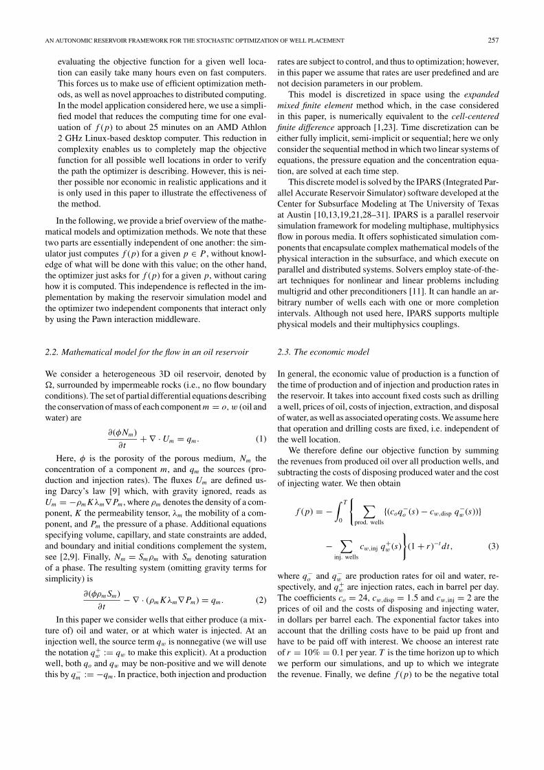
Figure 1. Permeability field showing the positions of current wells. The symbols ‘∗’ and ‘+’ indicate injection and producer wells, respectively.

independent, they could well be run in parallel, for exampleon two different clusters. Given the high cost of running eachof these simulations, this can reduce the run-time by a factorof two. Also, there are modifications of the basic SPSA al-gorithm that not only compute one search direction �k andevaluate the objective function in forward and backward di-rection, but rather generate several, say S search directions,resulting in 2S function evaluations [25]. The final update stepfrom pk to pk+1 is then done by incorporating the informationof all these computations. This modification allows a better ap-proximation of the true gradient of f (·) and will thus convergein less iterations. The cost of additional function evaluationscould be buffered by running some or all of the independent2S IPARS computations in parallel, a task which the IPARSFactory (to be described below) could easily distribute to avail-able resources. Finally, by starting at different initial points,the algorithm may converge to the same optimum solution(augmenting the reliability of reaching a unique global solu-tion) or to a set of different solutions (several extrema due tothe nonlinearity of the problem). In the latter case, specialistsand management could be interested in looking at clusters ofsolutions for comparison against other complex factors notincluded during the optimization stage. We have not yet im-plemented these extensions to the basic SPSA algorithm, butplan to explore them in a future work.

2.5. Case study

In our case study we consider a 2D reservoir � = [0, 4880]×[0, 5120] of roughly 25 million ft2, which is discretized by

a 61 × 64 spatial grid of 80 ft spacing along each horizontaldirection, and a depth of 30 ft. Hence, the model consistsof 3904 gridblocks. The reservoir under study is located ata depth of 3868.94 ft (i.e., 1 km) and corresponds to a 2Dsection extracted from the Gulf of Mexico. The porosity hasbeen fixed at φ = 0.2 but the reservoir has a heterogeneouspermeability field as shown in figure 1. The fluids are initiallyin equilibrium with water pressures set to 2600 psi and oilsaturation to 0.7.

The original reservoir consists of 5 wells: 2 water injectorsand 3 oil producers. Figure 1 shows the opposite-corner dis-tribution of injectors (bottom left) and producers (top right).Injection and production rates are computed by specifying afixed bottom hole pressure (BHP). Since oil flows from thelower left corner to the upper right corner, one would intu-itively guess that the new injection well should be locatedsomewhere in the neighborhood of the reservoir center. Thepermeability field suggests that flow should be faster in thelower part of the reservoir, so the new well should shift itslocation to the upper part, where oil is displaced more slowly.This is also indicated by looking at the oil saturation and pres-sures at the end of the simulation period at T = 2000 days, asshown in figure 2. However, such analysis is not that straight-forward when more wells are involved.

Given this description of the domain, the parameterspace is the set of 3904 points of the integer lattice P ={40, 80, 120, . . . , 4840} × {40, 80, 120, . . . , 5080} of cellmidpoints, at which we can place wells in our computationalmodel. We assume that the well penetrates through the entiredepth of the reservoir, that is, the depths of its bottom andtop are fixed. We also fix the BHP operating conditions at the

260 BANGERTH ET AL.

Figure 2. Top: Oil saturation at the end of the simulation for the original well distribution. Bottom: Oil pressure.

new injection well to be the same as that at the other injectionwells. We note that in general, the BHP and well penetrationparameter could vary and become an element of P . Also, morewells could be placed.

The goal of the case study is then to find the optimal posi-tion p ∈ P of a new well, with respect to the objective functionf (p) defined above. Given enough computing resources, one

could evaluate f (p) for all 3904 possible p ∈ P and from thiseasily determine the optimal well location. For the simple testcase considered here where every function evaluation takesabout 25 min on a Linux PC consisting of dual 2 GHz AMDAthlon processors, we have actually done this and show theresults in figure 3. However, for more realistic computations,this is of course not possible, and optimization algorithms

AN AUTONOMIC RESERVOIR FRAMEWORK FOR THE STOCHASTIC OPTIMIZATION OF WELL PLACEMENT 261

Figure 3. Search space response surface: Expected revenue − f (p) for all possible well locations p ∈ P . White marks indicate optimal well locations foundby SPSA for 7 different starting points of the algorithm.

have to use much less than this number of function evalua-tions. In this paper we achieve this using the SPSA algorithmdiscussed above.

Note that while we would in general like to compute theglobal optimum, we will usually be content if the algorithmfinds a solution that is almost as good. This is important inthe present context where the revenue surface plotted in fig-ure 3 has 72 local optima, with the global optimum beingf (p = {2920, 920}) = −1.09804 · 108. However, there are 5more local extrema within only half a per cent of this optimalvalue, which makes finding the global optimum rather com-plicated. The white marks in the figure indicate the best wellpositions found by the SPSA algorithm when started fromseven different points on the top-left to bottom-right diagonalof the domain. As can be seen, SPSA is able to find very goodwell locations from arbitrary starting points, even though itdoes not find the global optimum every time.

3. Enabling autonomic oil reservoir optimization usingdecentralized services

The overall application scenario is illustrated in figure 4. Theprimary peers and services participating in the application aredescribed below.

3.1. Integrated Parallel Accurate Reservoir Simulator(IPARS)

IPARS is the reservoir simulator that, together with the eco-nomic model, is used to evaluate the objective function. It is

a peer in our application that takes a number of input fileswhich, among other things, specify a well position p, andreturns the production history of all wells. IPARS is primar-ily implemented in Fortran and C, but is integrated with theframework discussed in this paper using C++ wrappers andthe Java Native Interface.

3.2. IPARS factory

The IPARS Factory is responsible for configuring instancesof IPARS simulations, deploying them on resources on theGrid, and managing their execution. Configuration consistsof generating the relevant input files that select appropriatemodels from those provided by IPARS, define the structureand properties of the reservoir to be simulated, and list requiredparameters. Deployment and management of IPARS instancesuse services provided by Discover [14] and Globus [6], andbuild on the CORBACoG Kit [18].

3.3. SPSA optimization service

The SPSA Optimization service runs on the Optimization peerand implements the SPSA algorithm presented in Section 2.4.It also offers interfaces and mechanisms for interactive andautonomic communications between the Optimization peer,IPARS instances, and the IPARS Factory. The optimizationservice uses the SPSA algorithm to generate guesses of newwell positions. This guess is first compared against an archiveof already computed well positions, therefore preventing use-less computation of already known data. If no match is found,

262 BANGERTH ET AL.

Figure 4. Autonomous oil reservoir optimization using decentralized services.

the new guess is added to the archive and is forwarded tothe IPARS Factory. The IPARS factory then uses these wellpositions to initialize and configure a new instance of IPARS.

3.4. Economic modeling service

The Economic Modeling Service is based on the eco-nomic model presented in Section 2.3 and uses the out-put produced by an IPARS simulation instance and cur-rent market parameters (e.g. oil prices, drilling costs, etc.)to compute estimated revenues for a particular reservoirconfiguration.

The market parameters used by the model are variableeconomic indices including the price of oil per volume pro-duced, the cost of water per volume, the cost of disposal ofwater, and the current discount rate. These indices are ob-tained using a network information service that collects in-formation at regular intervals from different sources on theInternet. The network information service is implementedas a threaded Java Servlet and is part of the Discover mid-dleware. The Servlet essentially queries a relevant URL(e.g. http://money.cnn.com/markets/commodities.html), andparses the responses to extract current oil, gas and water prices.This information is then fed into the economic model duringthe optimization process.

In general, instead of fixed current prices obtained by thenetwork information services, one may be able to use a set of“forecasts” of prices, delivered by stochastic or other math-

ematical models. This would allow a more realistic planningof future revenues from an oil field. However, this capabilityis not currently implemented and is not a part of the prototypeapplication.

3.5. Discover computational collaboratory

Discover [14] is a virtual, interactive computational collab-oratory that provides services to enable geographically dis-tributed scientists and engineers to collaboratively monitorand control high performance parallel/distributed applicationson the Grid. Its primary goal is to bring Grid applicationsto the scientists’/engineers’ desktops, enabling them to col-laboratively access, interrogate, interact with, and steer theseapplications using pervasive portals. Key components of theDiscover collaboratory include:

� Discover Interaction & Collaboration Middleware Sub-strate [3] that enables global collaborative access to mul-tiple, geographically distributed instances of the Discovercomputational collaboratory, and provides interoperabilitybetween Discover and external Grid services. The middle-ware substrate enables Discover interaction and collabo-ration servers to dynamically discover and connect to oneanother to form a peer network. This allows clients con-nected to their local servers to have global access to allapplications and services across all servers based on theircredentials, capabilities and privileges.

AN AUTONOMIC RESERVOIR FRAMEWORK FOR THE STOCHASTIC OPTIMIZATION OF WELL PLACEMENT 263

Figure 5. Pawn architecture: Pawn builds on network and interaction services to enable P2P interactions in Grid applications.

The Discover middleware also integrates Discover col-laboratory services with the Grid services provided by theGlobus Toolkit [6] using the CORBA Commodity Grid(CORBA CoG) Kit [18]. Clients can use the servicesprovided by the CORBA CoG Kit to discover availableresources on the Grid, to allocate required resources, torun applications on these resources, and use Discover toconnect to and collaboratively monitor, interact with, andsteer the applications.

� DIOS Interactive Object Framework (DIOS) [12,16] thatenables the runtime monitoring, interaction and compu-tational steering of parallel and distributed applicationson the Grid. DIOS enables application objects to be en-hanced with sensors and actuators so that they can beinterrogated and controlled. Application objects may bedistributed (spanning many processors) and dynamic (becreated, deleted, changed or migrated at runtime). A con-trol network connects and manages the distributed sensorsand actuators, and enables their external discovery, interro-gation, monitoring and manipulation. The control networkenables sensors and actuators to be encapsulated within,and directly deployed with the computational objects. TheDIOS distributed rule engine allows users to remotely de-fine and deploy rules and policies at runtime and enablesautonomic monitoring and steering of Grid applications.

� Discover Collaborative Portals [14] that provide the ex-perts (scientists, engineers) with collaborative access toother peer components. Using these portals, experts candiscover and allocate resources, configure and launchpeers, and monitor, interact with, and steer peer execution.The portal provides a replicated shared workspace archi-tecture and integrates collaboration tools such as chat andwhiteboard. It also integrates “Collaboration Streams,”that maintain a navigable record of all client-client andclient-applications interactions and collaboration.

3.6. Pawn peer-to-peer messaging framework

Pawn builds on Project JXTA [22] and enables peers to ex-change messages through common services and interactionmodes. Figure 5 shows the services and interaction modali-ties enabled by the Pawn framework.

Pawn offers four key services to enable dynamic collab-orations and autonomic interactions in scientific computingenvironments.

The Application Runtime and Control [ARC] announces theexistence of an application to the peergroup, sends applica-tion responses, publishes application update messages, andnotifies the peergroup of an application termination.

The Application Monitoring and Steering Service [AMS] en-ables users to interact with an application in real-time. Us-ing the AMS service a user can monitor, retrieve, or setapplication data.

The Application Execution Service [AEX] enables a peer toremotely start, stop, get the status of, or restart an appli-cation. This service requires a mechanism that supportssynchronous and guaranteed remote calls necessary for re-source allocation and application deployment (i.e. transac-tion oriented interactions) in a P2P environment.

The Collaboration Service [Group Communication,Presence] extends the Discover substrate to providecollaborative tools and support for group communicationand detection of presence.

Every peer can implement all or a subset of these services.Particular services subsets characterize a role for the peer.There are three distinct roles that a peer can take:

Client Peer that can deploy applications on available resourcesfor monitoring and/or steering; the client can also collab-orate with other peers in the group using Chat and White-board tools.

Application Peer that exports the application interfaces andcontrols to the peergroup; these interfaces are used by otherpeers to interact with the application. An application mayalready be enabled to communicate remotely with a middle-ware server as in the Discover computational collaboratory[14]; in such a case, the application peer acts as a proxypeer, relaying queries and responses to and from clients toapplications.

Rendezvous Peer to distribute or relay messages. Rendezvouspeers filter messages as defined by filtering rules input fromthe connected clients. The communication uses TCP unicastmessages between endpoints to establish one-to-one andone-to-many delivery modes.

264 BANGERTH ET AL.

Using the Pawn and Discover computational collaboratory,clients can connect to a local server using the portal, and canuse it to discover and access active applications and serviceson the Grid as long as they have appropriate privileges andcapabilities. Furthermore, they can form or join collaborationgroups and can securely, consistently, and collaboratively in-teract with and steer applications based on their privilegesand capabilities. The components described above need todynamically discover and interact with one another as peersto achieve the overall application objectives. As can be seenin figure 4, the experts use the portals to interact with theDiscover middleware and the Globus Grid services to dis-cover and allocate appropriate resource, and to deploy theIPARS Factory, SPSA and Economic Model peers (Step 1).The IPARS Factory discovers and interacts with the SPSAservice peer to configure and initialize it (Step 2). The expertinteracts with the IPARS Factory and SPSA to define appli-cation configuration parameters (Step 3). The IPARS Factorythen interacts with the Discover middleware to discover andallocate resources and to configure and execute IPARS sim-ulations (Step 4). The IPARS simulation now interacts withthe Economic Model to determine current revenues, and dis-covers and interacts with the SPSA service when it needsoptimization (Step 5). SPSA provides the IPARS Factorywith a new guess for a better well location (Step 6), whichthen uses it to configure and launch new IPARS simulations(Step 7). Experts can, at anytime, discover, collaborativelymonitor, and interactively steer IPARS simulations, configurethe other services, and drive the scientific discovery process(Step 8). Once the optimal well parameters are determined, theIPARS Factory configures and deploys a production IPARSrun.

These interactions are enabled by the Pawn services thatbuild on JXTA’s pipe and resolver services to provide statefuland guaranteed messaging. In Pawn, messages are platform-independent, and are composed of source and destinationidentifiers, a message type, a message identifier, a payload,and a handler tag. State is maintained by making every mes-sage a self-sufficient and self-describing entity that carriesenough information such that, in case of a link failure, it canbe resent to its destination by an intermediary peer withoutthe need to be recomposed by its original sender. In addition,messages can include system and application parameters inthe payload to maintain application state.

Pawn implements application-level communication guar-antees by combining stateful messages, message queueing,and a per-message acknowledgment table maintained at ev-ery peer. This messaging is used to enable the key application-level interactions such as :

Synchronous/Asynchronous Communication: Communica-tion in JXTA can be synchronous (using blocking pipes)or asynchronous (using non-blocking pipes or the resolverservice). In order to provide reliable messaging, Pawn com-bines these communication modalities with stateful mes-saging and guarantee mechanism.

Dynamic Data Injection: Pawn leverages JXTA pipes mecha-nisms and combines it with its guaranteed message deliverymechanism to provide Dynamic Data Injection.

Remote Procedure Calls (PawnRPC): The PawnRPC mecha-nism provides the low-level constructs for building appli-cations interactions across distributed peers. Using Pawn-RPC, a peer can dynamically invoke a method on a remotepeer by passing its request as an XML message through apipe.

4. Reservoir optimization using the pawn framework

In this section, we describe how Pawn is used to support theprototype autonomic oil reservoir optimization applicationoutlined in Section 2. Every interacting component is a peerthat implements Pawn services. The IPARS Factory, SPSA,and the Discover collaboratory are Application peers and im-plement ARC and AEX services. The Discover portals areClient peers and implement AMS and Group communicationservices. Key operations in the process include peer deploy-ment (e.g. IPARS Factory deploys IPARS), peer discovery(e.g IPARS Factory discovers SPSA), peer initialization andconfiguration (e.g. Expert configures SPSA), autonomic op-timization (e.g IPARS and SPSA interactively optimize rev-enue), interactive monitoring and steering (e.g. Experts con-nect to, monitor, and steer IPARS), and collaboration (e.g.Experts collaborate with one another). These operations aredescribed below.

4.1. IPARS factory and SPSA optimization servicedeployment

The IPARS Factory and SPSA Optimization peers aredeployed using Globus services accessed through Dis-cover/CORBACoG. The SPSA peer is a C++ program that isintegrated with Pawn using the Java Native Interface. Figure 6presents the sequence of operations involved. The deploymentis orchestrated by the Expert through the Discover portal. Theportal gives the Expert secure access to all the machines reg-istered with Globus Meta Directory Service (MDS) to whichthe Expert has access privileges. Authentication and autho-rization is based on the Globus Grid Security Infrastructure(GSI) service. Once authenticated, the Expert can use the por-tal to deploy the IPARS Factory and SPSA peers on machinesof choice after verifying their availability and current status(load, CPU, memory). Deployment uses the Globus GRAMservice. The portal also gives the Expert access to already de-ployed services and applications for collaborative monitoringand steering using Discover.

4.2. Peer initialization and discovery

At startup, peers use the underlying JXTA discovery service topublish an advertisement to the peergroup. This advertisement

AN AUTONOMIC RESERVOIR FRAMEWORK FOR THE STOCHASTIC OPTIMIZATION OF WELL PLACEMENT 265

Figure 6. Peer deployment.

describes the functionalities and services offered by the peer.It also contains a pipe advertisement for input and outputcommunications, and the RPC interfaces offered by the peerfor remote monitoring, steering, service invocation and man-agement. To enable peers to mutually identify each other,the peer that discovers an advertisement sends its adver-tisement back to the discovered peer. This discovery pro-cess is also used by IPARS instances to discover the SPSAservice.

4.3. IPARS and SPSA configuration

The Expert uses the portal and the control interfaces exportedto configure the SPSA service and to define its operating pa-rameters. The Expert also configures the IPARS Factory byspecifying the parameters for IPARS simulations. The IPARSFactory uses these parameters to set up IPARS instances dur-ing the optimization process, and initialize the SPSA service.Note that the Expert can always use the interaction and con-trol interfaces to modify these configurations. The configura-tion uses AMS to send application parameters to the IPARSFactory and SPSA peer. A response is generated and sentback (using AEX) to the client to confirm the configurationchange.

4.4. Oil reservoir optimization

The reservoir optimization process consists of two phases,an initialization phase and an iterative optimization phase asdescribed below.

Initialization phase: In the initialization phase, SPSA providesthe IPARS Factory with an initial guess of well parametersbased on its configuration by the Expert and the IPARS

Factory. This is done using the channel established duringdiscovery and is used by the IPARS Factory to initializeand deploy an IPARS instance.

Iterative optimization phase: In the iterative optimizationphase, the IPARS instance uses the Economic Model alongwith current market parameters to estimate the current rev-enue f (p) for the trial well locations p. SPSA uses thisvalue to generate an updated guess of the well parameterspk+1. It then sends new trial well locations to the IPARSFactory. The IPARS Factory now configures a new instanceof IPARS with the updated well parameters and deploys it.This process continues until the required terminating con-dition is reached. Figure 7 shows the overall optimizationprocess between IPARS Factory, IPARS, and SPSA. Notethat experts can connect to any of these peers at any timeand steer the optimization process.

Well parameter and revenue archive: After each evaluation ofa trial well location, these well parameters and the corre-sponding revenue computed by IPARS and the EconomicModel are stored in an archive (a MySQL database) main-tained by an archival peer. During the optimization pro-cess, when a new trial location is received from SPSA,the IPARS Factory checks the archive before launching anIPARS instance. If the current location is already presentin the archive, the corresponding normalized revenue valueis sent back to SPSA and a redundant IPARS instance isavoided.

Note that peer interactions during the optimization pro-cess are highly dynamic and require synchronous or asyn-chronous RPC semantics with guarantees, rather than doc-ument exchanges typically supported by P2P systems. InPawn, these interactions are enabled by PawnRPC, whichprovides the same semantics as the traditional RPC in a

Figure 7. Optimization process.

266 BANGERTH ET AL.

Figure 8. Graphical user interface of the Expert’s portal.

Figure 9. Computed well positions and economic revenue during the optimization process.

client-server system, but is implemented in a purely P2Pmanner.

4.5. Production runs and collaborative monitoring andsteering

Once the optimization process terminates and the optimalwell parameters are determined, the IPARS Factory allo-cates appropriate resources, configures a production run basedon these parameter, and launches this run on the allocatedresources.

Experts can now collaboratively connect to the running ap-plication, collectively monitor its execution and interactivelysteer it. Figure 8 presents the client peer’s portal interface usedby the Experts. The portal interface can also be used to access,

monitor and steer the IPARS Factory, the SPSA Optimizationservice, and the Economic Model.

4.6. Sample results from the oil reservoiroptimization process

Sample results from the oil reservoir optimization processare shown in figures 3 and 9. The first shows the computedrevenue for each possible well location, and the points whichSPSA chooses as optimal well locations for a number of differ-ent initial guesses. Figure 9 shows the path the SPSA iteratestake for a particular initial guess. Note that, in general, startingat different initial values yields different end points, which isnot suprising given that the shown surface has 72 local optima.However, in all cases we investigated, the found optimum is

AN AUTONOMIC RESERVOIR FRAMEWORK FOR THE STOCHASTIC OPTIMIZATION OF WELL PLACEMENT 267

within half a per cent of the global one. In view of this, thealgorithm performs very favorably and took on average only25–30 iterations to converge.

5. Policy-driven reservoir optimization

A key objective of the research presented in this paper is toformulate policies that can be used by the autonomic self-optimizing reservoir framework to discover, select, configure,and invoke appropriate optimization services to determine op-timal well locations.

The choice of optimization service depends on the sizeand nature of the reservoir. The SPSA algorithm studied inthis paper is suited for larger reservoirs with relatively smoothcharacteristics. In case of reservoirs with many randomly dis-tributed maxima and minima, the VFSA algorithm studied inour previous paper [15] can be employed during the initial op-timization phase. Once convergence slows down, VFSA canbe replaced by SPSA. Alternate optimization schemes (e.g.,genetic algorithms, local methods such as Newton) can alsobe used if convergence breaks down. We plan to study andcharacterize the behavior and interaction of these schemes ina future work.

Similarly, policies can also be used to manage the be-havior of the reservoir simulator. For example, the policymay monitor convergence of the optimizer and as it ap-proaches the solution, it may use a finer mesh and/or smallertimesteps. The policy may even attempt to activate other nu-merical algorithms (e.g., time discretization schemes, solvers)or physical models (e.g., one-, two-, or three-phase flow, ge-omechanical). Moreover, the policy may replace IPARS bysome other simulator capable of using unstructured grids oradaptive mesh refinement in order to generate more accuratesimulations.

In an alternative scenario, policies may be defined to en-able various optimizers to execute concurrently on dynam-ically acquired Grid resources, and select the best well lo-cation among these based on some metric (e.g., estimatedrevenue, time or cost of completion). This aspect is impor-tant for speeding up the search, or for studying the effects ofparameters that were not included at the start of the optimiza-tion. For instance, some topological difficulties or unforeseencosts for drilling a well may eventually arise in some parts ofthe reservoir. In such a case, the expert may decide to stopthe process based on a small set of nearly optimal solutionsor perturb the course of the optimization (e.g. by the intro-duction or removal of decision variables, constraints or trialpoints).

The autonomic reservoir framework and the underlyingPawn peer-to-peer middleware substrate presented in this pa-per enable the decoupling of services and the separation ofpolicy and mechanism. This allows external policies, suchas those outlined above, to be dynamically defined and usedto manage the behavior of the components/services, and toorchestrate interactions between them to achieve overall op-timization goals of the reservoir.

6. Summary and conclusions

In this paper we presented the design, development, and op-eration of a prototype autonomic self-optimizing reservoirframework that uses peer-to-peer interactions between ap-plications and services on the Grid to enable the autonomicoptimization of well placement and operation to maximizeoverall revenue. The application consisted of instances of dis-tributed multi-model, multi-block reservoir simulation com-ponents provided by IPARS, stochastic optimization servicesprovided by SPSA, economic modeling services, real-timeservices providing current economic data (e.g. oil prices),archives for already computed data, and experts (scientists,engineers) connected via pervasive collaborative portals. Itwas built on the Pawn P2P substrate, which provided JXTA-based peer-to-peer messaging services, and the Discover com-putational collaboratory, which combines Grid infrastructureservices provided by Globus and interaction and collabora-tion services. Sample outputs from the optimization processwere presented that showed how the interaction of all thesecomponents can be used to solve the economically impor-tant question of where to place a new well into an existingreservoir. This problem is computationally very challengingdue to the enormous complexity of optimizing a complicatedmathematical model, and can benefit from the distributed andautonomous features of the approach presented here. Further-more, the formulation of policies for the autonomic selec-tion, configuration and invocation of optimization services arenecessary ingredients of adaptively changing the componentsused in the optimization.

The prototype autonomic Grid application presented inthis paper demonstrated the potential of the emerging Gridinfrastructure and its support for secure and seamless interac-tions, enabling a new generation of autonomic applications.These applications will be based on peer-to-peer interactionsbetween application components, Grid services, resources,and data, and will use separately defined policies to orches-trate these interactions and enable self-managing and self-optimizing behaviors. We believe that such autonomic behav-iors will be critical for addressing the scale, complexity, het-erogeneity and dynamism inherent in Grid applications andenvironments.

Acknowledgments

The research presented in this paper is supported in part bythe National Science Foundation (NSF) via grants numbersACI 9984357 (CAREERS), EIA 0103674 (NGS), NSF EIA-0121523/EIA-0120934 (ITR), ANI-0335244 (NRT), CNS-0305495 (NGS) and by DOE ASCI/ASAP (Caltech) via grantnumber 82-1052856.

References

[1] T. Arbogast, M.F. Wheeler and I. Yotov, Mixed finite elements for ellip-tic problems with tensor coefficients as cell-centered finite differences,SIAM J. Numer. Anal 34(2) (1997) 828–852.

268 BANGERTH ET AL.

[2] K. Aziz and A. Settari, Petroleum Reservoir Simulation (Applied Sci-ence Publishers Ltd., London, 1979).

[3] V. Bhat and M. Parashar, Discover middleware substrate for integratingservices on the grid, in: Proceedings of the 10th International Confer-ence on High Performance Computing (HiPC 2003), eds. T.M. Pinkstonand V.K. Prasanna, volume 2913 of Lecture Notes in Computer Science,Springer-Verlag, (Dec. 2003) pp. 373–382.

[4] A.C. Bittencourt and R.N. Horne, Reservoir development and designoptimization, in: SPE Annual Technical Conference and Exhibition,San Antonio, Texas, (Oct. 1997) SPE 38895.

[5] G. Chavent and J. Jaffre, Mathematical Models and Finite Elements forReservoir Simulation (North-Holland, Amsterdam, 1986).

[6] I. Foster and C. Kesselman, (eds.), Globus: A Toolkit Based Grid Ar-chitecture, Morgan Kaufman, (1999) pp. 259–278.

[7] I. Foster and C. Kesselman, The Grid 2: Blueprint for a New ComputingInfrastructure (Morgan Kaufman, 2004).

[8] B. Guyaguler and R.N. Horne, Uncertainty assessment of well place-ment optimization, in: SPE Annual Technical Conference and Exhibi-tion (New Orleans, Louisiana, September, 2001). SPE 71625.

[9] R. Helmig, Multiphase Flow and Transport Processes in the Subsurface(Springer, 1997).

[10] IPARS: Integrated Parallel Reservoir Simulator, http://www.ices.utexas.edu/CSM.

[11] S. Lacroix, Y. Vassilevski and M.F. Wheeler, Iterative solvers of the im-plicit parallel accurate reservoir simulator (IPARS), Numerical LinearAlgebra with Applications 4 (2001) 537–549.

[12] H. Liu and M. Parashar, DIOS++: A framework for rule-based auto-nomic management of distributed scientific applications, in: Proceed-ings of the 9th International Euro-Par Conference (Euro-Par 2003),eds. H. Kosch, L. Boszormenyi and H. Hellwagner, volume 2790 ofLecture Notes in Computer Science, Springer Verlag (2003), pp. 66–73.

[13] Q. Lu, M. Peszynska and M.F. Wheeler, A parallel multi-block black-oil model in multi-model implementation, SPE Journal 7(3) (2002)278–287, SPE 79535.

[14] V. Mann, V. Matossian, R. Muralidhar and M. Parashar, DISCOVER:An environment for Web-based interaction and steering of high-performance scientific applications, Concurrency and Computation:Practice and Experience 13(8/9) (2001) 737–754.

[15] V. Matossian, V. Bhat, M. Parashar, M. Peszynska, M. Sen, P. Stoffa andM.F. Wheeler, Concurrency and Computation: Practice and Experience,John Wiley and Sons, Vol. 17, Issue 1, pp. 1–26, 2005.

[16] R. Muralidhar and M. Parashar, A distributed object infrastructure forinteraction and steering, Concurrency and Computation: Practice andExperience 15(10) (2003) 957–977.

[17] Y. Pan and R.N. Horne, Improved methods for multivariate optimizationof field development scheduling and well placement design, in: SPEAnnual Technical Conference and Exhibition, New Orleans, Louisiana,(Sept. 1998) pp. 27–30. SPE 49055.

[18] M. Parashar, G. von Laszewski, S. Verma, K. Keahey J. Gawor andN. Rehn, A CORBA commodity grid kit, Special Issue on Grid Com-puting Environments, Concurrency and Computation: Practice and Ex-perience 14 (2002) 1057–1074.

[19] M. Parashar, J.A. Wheeler, G. Pope, K. Wang and P. Wang, A newgeneration EOS compositional reservoir simulator, Part II: Frameworkand multiprocessing, in: Fourteenth SPE Symposium on Reservoir Sim-ulation, Dallas, Texas, Society of Petroleum Engineers (June 1997) pp.31–38.

[20] D.W. Peaceman, Fundamentals of Numerical Reservoir Simulation, 1stedition (Elsevier Scientfic Publishing Company, Amsterdam-Oxford-New York, 1977).

[21] M. Peszynska, Q. Lu and M.F. Wheeler, Multiphysics coupling of codes,in: Computational Methods in Water Resources, eds., L.R. Bentley, J.F.Sykes, C.A. Brebbia, W.G. Gray and G.F. Pinder, A. A. Balkema (2000)pp. 175–182.

[22] Project JXTA: http://www.jxta.org, 2001.

[23] T.F. Russell and M.F. Wheeler, Finite element and finite differencemethods for continuous flows in porous media, in: The Mathematics ofReservoir Simulation, ed., R.E. Ewing, SIAM, Philadelphia (1983) pp.35–106.

[24] M. Sen and P. Stoffa, Global Optimization Methods in GeophysicalInversion (Elsevier, 1995).

[25] J.C. Spall, Multivariate stochastic approximation using a simultaneousperturbation gradient approximation, IEEE Trans. Autom. Control 37(1992) 332–341.

[26] J.C. Spall, Adaptive stochastic approximation by the simulateousperturbation method, IEEE Trans. Autom. Contr 45 (2000) 1839–1853.

[27] J.C. Spall, Introduction to Stochastic Search and Optimization: Esti-mation, Simulation and Control, Inc., Publication, John Wiley & Sons,New Jersey (2003).

[28] P. Wang, I. Yotov, M.F. Wheeler, T. Arbogast, C.N. Dawson,M. Parashar and K. Sepehrnoori, A new generation EOS composi-tional reservoir simulator. Part I: Formulation and discretization, in:Fourteenth SPE Symposium on Reservoir Simulation, Dallas, Texas,Society of Petroleum Engineers (June 1997) pp. 55–64.

[29] M.F. Wheeler and M. Peszynska, Computational engineering and sci-ence methodologies for modeling and simulation of subsurface appli-cations, Advances in Water Resources, in press.

[30] M.F. Wheeler, M. Peszynska, X. Gai and O. El-Domeiri, Modelingsubsurface flow on PC cluster, in: High Performance Computing, ed.A. Tentner, SCS (2000) pp. 318–323.

[31] M.F. Wheeler, J.A. Wheeler and M. Peszynska, A distributed comput-ing portal for coupling multi-physics and multiple domains in porousmedia, in: Computational Methods in Water Resources, (eds.), L.R.Bentley, J.F. Sykes, C.A. Brebbia, W.G. Gray, and G.F. Pinder, A. A.Balkema, (2000) pp. 167–174.

[32] B. Yeten, L.J. Durlofsky and K. Aziz, Optimization of nonconventionalwell type, location, and trajectory, SPE Journal 8(3) (2003) 200–210.SPE 86880.

Wolfgang Bangerth is a postdoctoral research fel-low at both the Institute for Computational Engi-neering and Sciences, and the Institute for Geo-phyics, at the University of Texas at Austin. He ob-tained his Ph.D. in applied mathematics from theUniversity of Heidelberg, Germany in 2002. He isthe project leader for the deal.II finite element li-brary (http://www.dealii.org). Wolfgang is a mem-ber of SIAM, AAAS, and ACM.E-mail: bangerth@ices.utexas.edu

Hector Klie obtained his Ph.D. degree in Computa-tional Science and Engineering at Rice University,1996, he completed his Master and undergraduatedegrees in Computer Science at the Simon Boli-var University, Venezuela in 1991 and 1989, re-spectively. Hector Klie’s main research interestsare in the development of efficient parallel linearand nonlinear solvers and optimization algorithmsfor large-scale transport and flow of porous mediaproblems. He currently holds the position of As-sociate Director and Senior Research Associate inthe Center for Subsurface Modeling at the Instituteof Computational Science and Engineering at TheUniversity of Texas at Austin. Dr. Klie is currentmember of SIAM, SPE and SEG.E-mail: klie@ices.utexas.edu

AN AUTONOMIC RESERVOIR FRAMEWORK FOR THE STOCHASTIC OPTIMIZATION OF WELL PLACEMENT 269

Vincent Matossian obtained a Masters in appliedphysics from the French Universite Pierre et MarieCurie. Vincent is currently pursuing a Ph.D. degreein distributed systems at the Department of Electri-cal and Computer Engineering at Rutgers Univer-sity under the guidance of Manish Parashar. His re-search interests include information discovery andad-hoc communication paradigms in decentralizedsystems.E-mail: vincentm@caip.rutgers.edu

Manish Parashar is Professor of Electrical andComputer Engineering at Rutgers University,where he also is director of the Applied Soft-ware Systems Laboratory. He received a BE de-gree in Electronics and Telecommunications fromBombay University, India and MS and Ph.D. de-grees in Computer Engineering from Syracuse Uni-versity. He has received the Rutgers Board ofTrustees Award for Excellence in Research (2004–2005), NSF CAREER Award (1999) and the EnricoFermi Scholarship from Argonne National Labo-ratory (1996). His research interests include auto-nomic computing, parallel & distributed comput-ing (including peer-to-peer and Grid computing),

scientific computing, software engineering. He isa senior member of IEEE, a member of the IEEEComputer Society Distinguished Visitor Program(2004–2007), and a member of ACM.E-mail: parashar@caip.rutgers.edu

Mary Fanett Wheeler obtained her Ph.D. atRice University in 1971. Her primary researchinterest is in the numerical solutions of par-tial differential systems with applications to flowin porous media, geomechanics, surface flow,and parallel computation. Her numerical workincludes formulation, analysis and implementa-tion of finite-difference/finite-element discretiza-tion schemes for nonlinear, coupled PDE’s as wellas domain decomposition iterative solution meth-ods. She has directed the Center for SubsurfaceModeling, The University of Texas at Austin, sinceits creation in 1990. Dr. Wheeler is recepient of theErnest and Virginia Cockrell Chair in Engineeringand is Professor in the Department of AerospaceEngineering & Engineering Mechanics and in theDepartment of Petroleum & Geosystems Engineer-ing of The University of Texas.