Introduction to EEG and MEG - Max Planck Society · EEG WS 2012/2013, Thomas R. Knösche Max Planck...
67
EEG WS 2012/2013, Thomas R. Knösche Max Planck Institute for Human Cognitive and Brain Sciences Introduction to EEG and MEG Thomas R. Knösche Max Planck Institute for Human Cognitive and Brain Sciences
Transcript of Introduction to EEG and MEG - Max Planck Society · EEG WS 2012/2013, Thomas R. Knösche Max Planck...

EEG WS 2012/2013, Thomas R. Knösche Max Planck Institute for Human Cognitive and Brain Sciences
Introduction to EEG and MEG
Thomas R. Knösche
Max Planck Institute
for Human Cognitive and
Brain Sciences

EEG WS 2012/2013, Thomas R. Knösche Max Planck Institute for Human Cognitive and Brain Sciences
History: Discovery of Biological Electricity
Luigi Galvani (1737-1798) "Ich secirte einen Frosch, präparierte ihn und legt ihn auf
einen Tisch, auf dem eine Electrisirmaschine stand, weit
von deren Conductor getrennt. Wie nun der eine von den
Leuten, die mir zur Hand gingen, mit der Spitze des
Skalpellmessers die inneren Schenkelnerven des Frosches
zufällig ganz leicht berührte, schienen sich alle Muskeln an
den Gelenken wiederholt derart zusammenzuziehen, als
wären sie anscheinend von heftigen tonischen Krämpfen
befallen. Der andere aber, welcher uns bei den
Electrizitätsversuchen behilflich war, glaubte bemerkt zu
haben, dass sich das ereignet hätte, während dem
Conductor der Maschine ein Funken entlockt wurde."
1789
Physician, anatomist, biophysicist

EEG WS 2012/2013, Thomas R. Knösche Max Planck Institute for Human Cognitive and Brain Sciences
History: Theory of Bioelectricity
• Foundations of
electrophysiology
• Discovery of
electrical activity in
nerves and
muscles (1848)
Emil Heinrich du Bois-Reymond
(1818-1896)

EEG WS 2012/2013, Thomas R. Knösche Max Planck Institute for Human Cognitive and Brain Sciences
History: Discovery of Human EEG
Hans Berger (1873-1941)
(published 1929)
1924

EEG WS 2012/2013, Thomas R. Knösche Max Planck Institute for Human Cognitive and Brain Sciences
EEG: Recording
Electrodes
Amplifier
Display
1929 2012

EEG WS 2012/2013, Thomas R. Knösche Max Planck Institute for Human Cognitive and Brain Sciences
EEG Electrodes
Shape
Material: gold (durable, no DC), silver/silver chloride (care
intensive, DC), tin (cheap)
Attachement
ring cup sponge
glue geodesic nets caps

EEG WS 2012/2013, Thomas R. Knösche Max Planck Institute for Human Cognitive and Brain Sciences
EEG Amplifiers
• differential amplifiers
• sometimes separated into pre- and main amplifiers
• integrated high pass filters
• high input impedances, minimal distance from head
• AD converter: discretization in time and voltage
ANT - high-density amplifier
Number of channels 32, 64, 128 and 256
Sampling frequency 256, 512, 1024 and 2048 Hz
Resolution 22 bit, 71.5 nV per bit
Input impedance > 1012 Ohm
Noise < 1.5 Vpp (at 100 Hz)
CMRR > 110 dB
Connection to PC fiber optic to PCI card or USB2

EEG WS 2012/2013, Thomas R. Knösche Max Planck Institute for Human Cognitive and Brain Sciences
Electrode placement
10-20 system (Jasper, 1958)
21 positions
10-10 system (Chatrian, 1985)
74 positions
10-5 system (Oostenveld 2001)
~300 positions
Geodesic nets (Tucker)
64, 128, 256, … positions

EEG WS 2012/2013, Thomas R. Knösche Max Planck Institute for Human Cognitive and Brain Sciences
Reference and Montage
• Unipolar (against nasion, mastoid, Cz, …)
• Average reference (against mean of all channels)
• Bipolar (e.g., neighbouring electrodes in ant.-post. direction,
homologuous electrodes between hemispheres)

EEG WS 2012/2013, Thomas R. Knösche Max Planck Institute for Human Cognitive and Brain Sciences
EEG Display and Analysis

EEG WS 2012/2013, Thomas R. Knösche Max Planck Institute for Human Cognitive and Brain Sciences
Spontaneous EEG
Alpha waves: ca. 10 Hz
Delta waves: ca. 0.5 – 4 Hz
Subdelta: < 0.5 Hz
Slow waves/ spindles
Beta/gamma waves: >12 Hz

EEG WS 2012/2013, Thomas R. Knösche Max Planck Institute for Human Cognitive and Brain Sciences
Spontaneous EEG - Interpretation
Normal EEG – adult, light sleep

EEG WS 2012/2013, Thomas R. Knösche Max Planck Institute for Human Cognitive and Brain Sciences
Spontaneous EEG - Interpretation
Epileptiform discharges Creutzfeld-Jacob disease, different stages
left delta
epileptiform discharges

EEG WS 2012/2013, Thomas R. Knösche Max Planck Institute for Human Cognitive and Brain Sciences
Artifacts
Biological artifacts
• Movement (esp. MEG)
• Eye movement
• Eye blink
• muscle
• cardiac
Technical artifacts
• Electrodes
• Drifts
• Picking up from environment

EEG WS 2012/2013, Thomas R. Knösche Max Planck Institute for Human Cognitive and Brain Sciences
Treatment of Artifacts
Rejection
• Contaminated epochs are rejected
Advantages
• simple
• no signal distortion
Drawbacks
• Loss of data (especially if number of
epochs is limited)
• Selection bias
• Extra task „do not move your eyes“ can
influence experiment.
Correction
• Artifacts will be mathematically
eliminated
Advantages
• Avoidance of disadvantages of
rejection
Drawbacks
• Signal can and will be distorted. Extent
of distortion difficult to quantify.

EEG WS 2012/2013, Thomas R. Knösche Max Planck Institute for Human Cognitive and Brain Sciences
Event-related Potentials
sampling
250-2000 Hz
10-1000,
typically
20-200
epochs
32-256
electrodes

EEG WS 2012/2013, Thomas R. Knösche Max Planck Institute for Human Cognitive and Brain Sciences
Event-related Potentials - Example
Musical phrasing musical culture
CZ
Source: Nan, Knösche & Friederici, 2006
Stimulus material is presented in 4 variants, which differ in
two two-stage factors..
German, phrased
Chinese, phrased
German, unphrased
Chinese, unphrased
II: 100 - 300 ms
0
0.5
1
1.5
2
2.5
3
3.5
4
4.5
5
Chinese music Western music
diffe
rence a
mplit
ude (
uV
)
Chinese musicians
German musicians

EEG WS 2012/2013, Thomas R. Knösche Max Planck Institute for Human Cognitive and Brain Sciences
Magnetoencephalography

EEG WS 2012/2013, Thomas R. Knösche Max Planck Institute for Human Cognitive and Brain Sciences
Magnetoencephalography
EEG WS 2012/2013, Thomas R. Knösche Max Planck Institute for Human Cognitive and Brain Sciences
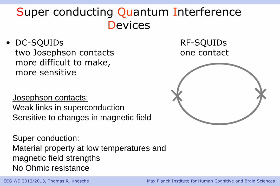
• DC-SQUIDs RF-SQUIDs two Josephson contacts one contact more difficult to make, more sensitive
Josephson contacts:
Weak links in superconduction
Sensitive to changes in magnetic field
Super conduction:
Material property at low temperatures and
magnetic field strengths
No Ohmic resistance
Super conducting Quantum Interference Devices

EEG WS 2012/2013, Thomas R. Knösche Max Planck Institute for Human Cognitive and Brain Sciences
Detector Coils
a) Magnetometers
b) Planar gradiometers 1. ord.
c) Radial gradiometers 1. ord.
d) Radial gradiometers 2. ord.

EEG WS 2012/2013, Thomas R. Knösche Max Planck Institute for Human Cognitive and Brain Sciences
Neuromag system
Three channels per chip
• Magnetometer
• Planar gradiometer
• Planar gradiometer

EEG WS 2012/2013, Thomas R. Knösche Max Planck Institute for Human Cognitive and Brain Sciences
Magnetometers and/or Gradiometers?

EEG WS 2012/2013, Thomas R. Knösche Max Planck Institute for Human Cognitive and Brain Sciences
MEG-Lab Gantry Sensor 3D-Digitizer
Shielded room
Stretcher

EEG WS 2012/2013, Thomas R. Knösche Max Planck Institute for Human Cognitive and Brain Sciences
The Forward Problem
Thomas R. Knösche
Max Planck Institute
for Human Cognitive and
Brain Sciences

EEG WS 2012/2013, Thomas R. Knösche Max Planck Institute for Human Cognitive and Brain Sciences
The Forward Problem
R2
R1
R3
I U
Law of Ohm
I=U/R2
???
We know the source current,
and want to compute the
EEG/MEG.

EEG WS 2012/2013, Thomas R. Knösche Max Planck Institute for Human Cognitive and Brain Sciences
Description of Electromagnetic Fields
0 E
JH
D
0 B
EJ
ED
HB
Quasistatic Maxwell equations
0
03
0
00
||
)()(
4
1)(
xx
xdxx
xxxJx
03
0
00
||
)()(
4)( xd
xx
xxxJxB
Sensor location Source location

EEG WS 2012/2013, Thomas R. Knösche Max Planck Institute for Human Cognitive and Brain Sciences
Primary and Volume Currents
EJJ p
+
cell body
sink
source
synapse
+
Secondary/volume
currents Primary/ source currents

EEG WS 2012/2013, Thomas R. Knösche Max Planck Institute for Human Cognitive and Brain Sciences
Volume Conductor: What needs to be modelled?
EEG
MEG
Modelling MEG Modelling EEG
MEG: Only volume
currents within the skull
need to be considered.
EEG: Also volume
currents outside the skull
interior must be modelled.

EEG WS 2012/2013, Thomas R. Knösche Max Planck Institute for Human Cognitive and Brain Sciences
How to Describe the Head Geometry?
Spherical model
Simplest solution

EEG WS 2012/2013, Thomas R. Knösche Max Planck Institute for Human Cognitive and Brain Sciences
Spherical Head Model
MEG EEG
Skull interior
Skull
Scalp
Described by: sphere center (M), radii (R) , conductivities ()
R3
R1
M 1
R2 R1
M 1
2
3
EEG WS 2012/2013, Thomas R. Knösche Max Planck Institute for Human Cognitive and Brain Sciences
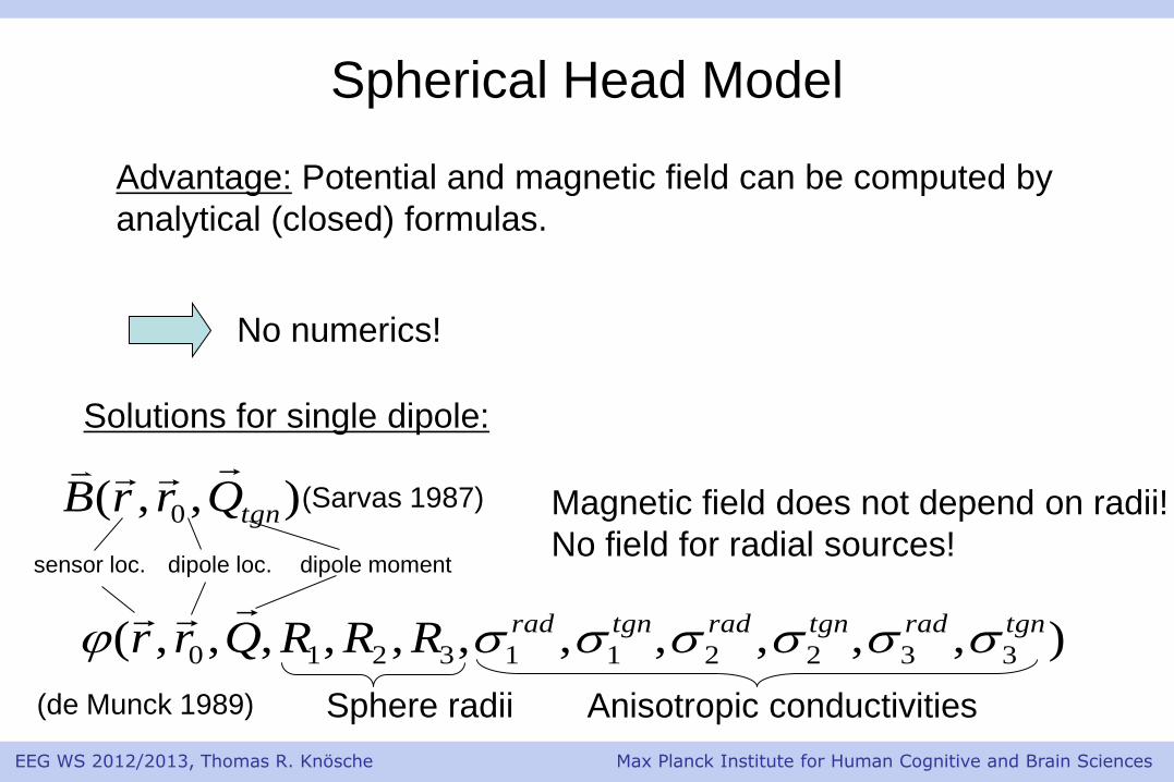
Spherical Head Model
Advantage: Potential and magnetic field can be computed by
analytical (closed) formulas.
No numerics!
),,( 0 tgnQrrB
Solutions for single dipole:
),,,,,,,,,,,( 3322113210
tgnradtgnradtgnradRRRQrr
sensor loc. dipole loc. dipole moment
Sphere radii Anisotropic conductivities
(Sarvas 1987)
(de Munck 1989)
Magnetic field does not depend on radii!
No field for radial sources!

EEG WS 2012/2013, Thomas R. Knösche Max Planck Institute for Human Cognitive and Brain Sciences
Spherical Head Model
fromTanzer, PhD thesis 2006
Electrical potential and magnetic field have orthogonal
topographies.
MEG
EEG

EEG WS 2012/2013, Thomas R. Knösche Max Planck Institute for Human Cognitive and Brain Sciences
Local Spherical Model
Dor each sensor a separate spher
is fitted to the local curvature of
the skull.

EEG WS 2012/2013, Thomas R. Knösche Max Planck Institute for Human Cognitive and Brain Sciences
Ellipsoidal Head Model
• Ellipsoids have more degrees of
freedom compared to spheres.
• Also ellipsoidal volume
conductors can be described
analytically .

EEG WS 2012/2013, Thomas R. Knösche Max Planck Institute for Human Cognitive and Brain Sciences
Boundary Elements Method (BEM)
• Realistic description of tissue
compartments with different
conductivities.
• Mostly: inner and outer skull
surface, outer head surface, but
also others, e.g. vetricles, CSF.
• Each compartment is described
by a homogeneous and isotropic
conductivity.

EEG WS 2012/2013, Thomas R. Knösche Max Planck Institute for Human Cognitive and Brain Sciences
Segmentation Grid generation
Boundary Elements Method (BEM)
EEG WS 2012/2013, Thomas R. Knösche Max Planck Institute for Human Cognitive and Brain Sciences
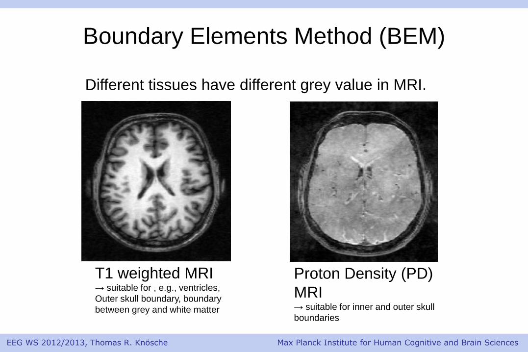
Different tissues have different grey value in MRI.
T1 weighted MRI → suitable for , e.g., ventricles,
Outer skull boundary, boundary
between grey and white matter
Proton Density (PD)
MRI → suitable for inner and outer skull
boundaries
Boundary Elements Method (BEM)

EEG WS 2012/2013, Thomas R. Knösche Max Planck Institute for Human Cognitive and Brain Sciences
Boundary Elements Methods (Conductivities)
1
2
3
• 1 - 3 are equivalent values
• true conductivities are
inhomogeneous and anisotropic
in each compartment.
• How to get these values?
• Usual choices: 1 = 0.33 S/m, 2
= 0.004 S/m, 3 = 0.33 S/m

EEG WS 2012/2013, Thomas R. Knösche Max Planck Institute for Human Cognitive and Brain Sciences
Finite Elements Method (FEM) Influence of anisotropic conductivity

EEG WS 2012/2013, Thomas R. Knösche Max Planck Institute for Human Cognitive and Brain Sciences
Finite Elements Method (FEM)
from Tanzer, PhD thesis2006
• Volume is divided into small
tetraedras or cubes.
• In every element one
conductivity tensor!
• Simultaneous solution of
Poisson‘s equation in all
elements, with boundary
conditions.

EEG WS 2012/2013, Thomas R. Knösche Max Planck Institute for Human Cognitive and Brain Sciences
Finite Elements Method (FEM) (Conductivities)
from Ramon et al (2006)
Values from Literature
However, no anisotropy DWI (see Tuch 2001)

EEG WS 2012/2013, Thomas R. Knösche Max Planck Institute for Human Cognitive and Brain Sciences
Finite Elements Method (FEM)
In principle, FEM is the ideal method, since all relevant volume
conductor properties can be accounted for, at any desired
resolution.
However …
• … it is still an unsolved problem to obtain these values in
real situations.
• … the computations demands are very high (however, recent
advances in fast solver technology seem to ameliorate this
problem, see Wolters et al. 2004)
• … the correct modeling of the source injection is still a
problem (Schimpf et al. 2002)

EEG WS 2012/2013, Thomas R. Knösche Max Planck Institute for Human Cognitive and Brain Sciences
Comparison of Methods
Analytical models (sphere, ellipsoid)
Advantages
• easy to implement, fast to compute
• no problems with model generation (no segmentation, grid
generation)
• analytical solution, no typically numerical problems, such as
accuracy, convergence, etc.
Drawbacks
• Heads are no balls! → Modelling error

EEG WS 2012/2013, Thomas R. Knösche Max Planck Institute for Human Cognitive and Brain Sciences
BEM models
Advantages
• Individual head geometry can be accounted for
• Relatively fast and economic solution
• No problems with source injection
Drawbacks
• Constant and isotropic conductivity in each compartment
• Inhomogeneities, such as skull holes or fontanelles/surtures
cannot be modelled and cause large errors.
Comparison of Methods

EEG WS 2012/2013, Thomas R. Knösche Max Planck Institute for Human Cognitive and Brain Sciences
FEM models
Advantages
• All relevant volume conductor properties can be accounted
for, at any desired resolution.
Drawbacks
• Material parameters difficult to obtain
• Possible numerical problems with source singularity.
• Model generation can be challenge.
Comparison of Methods

EEG WS 2012/2013, Thomas R. Knösche Max Planck Institute for Human Cognitive and Brain Sciences
Source Reconstruction
Thomas R. Knösche
Max Planck Institute
for Human Cognitive and
Brain Sciences

EEG WS 2012/2013, Thomas R. Knösche Max Planck Institute for Human Cognitive and Brain Sciences
Source Reconstruction
Measurement (EEG/MEG) Neuronal currents

EEG WS 2012/2013, Thomas R. Knösche Max Planck Institute for Human Cognitive and Brain Sciences
Source Reconstruction
Highly underdetermined
Measurement (EEG/MEG) Average currents in elements
of suitable size

EEG WS 2012/2013, Thomas R. Knösche Max Planck Institute for Human Cognitive and Brain Sciences
M L J = +
measurements
max. 430 values
lead field matrix (forward solution)
each column for 1 dipole
dipoles (3 per voxel)
several thousand values
noise

EEG WS 2012/2013, Thomas R. Knösche Max Planck Institute for Human Cognitive and Brain Sciences
Underdeterminedness Noise in data
Probability instead of certainty
Law of Bayes

EEG WS 2012/2013, Thomas R. Knösche Max Planck Institute for Human Cognitive and Brain Sciences
2
22
1exp)|( jLmjm
Extremely simple example:
one electrode, 2 dipoles
Likelihood
-2
-1.5
-1
-0.5
0 0
0.5
1
1.5
2
0
0.5
1
Likelihood

EEG WS 2012/2013, Thomas R. Knösche Max Planck Institute for Human Cognitive and Brain Sciences
object measurement
It is impossible to reconstruct the object just from the
shadow image
However: If we know that vases are in general rotationally symmetric and if we skip the
colouring, we can reconstruct an image that is similar to the original in important aspects.
Give up? Wait a minute ...

EEG WS 2012/2013, Thomas R. Knösche Max Planck Institute for Human Cognitive and Brain Sciences
2
2
1exp)( jjprior
Extremely simple example:
one electrode, 2 dipoles
A priori information
-2
-1.5
-1
-0.5
0 0
0.5
1
1.5
2
0
0.5
1
Prior

EEG WS 2012/2013, Thomas R. Knösche Max Planck Institute for Human Cognitive and Brain Sciences
A posteriori distribution – Bayes‘ law
)|()()|( jmjmj prior
-2
-1.5
-1
-0.5
0 0
0.5
1
1.5
2
0
0.5
1
Prior
-2
-1.5
-1
-0.5
0 0
0.5
1
1.5
2
0
0.5
1
Likelihood -2
-1.5
-1
-0.5
0 0
0.5
1
1.5
2
0
0.2
0.4
0.6
0.8
1Posterior

EEG WS 2012/2013, Thomas R. Knösche Max Planck Institute for Human Cognitive and Brain Sciences
A posteriori distribution – Bayes‘ law
)|()()|( jmjmj prior
Mostly, only the expectation of the posterior distribution is
computed:
)))|(log())(min(log(arg jmjj prior
Maximum a posteriori (MAP) estimator

EEG WS 2012/2013, Thomas R. Knösche Max Planck Institute for Human Cognitive and Brain Sciences
Where does a priori information come from
No information available – use mathematical constraints that select a
representative out of the class of possible solutions bearing maximum
likelihood
Specific qualitative function-anatomical knowledge
e.g. minimum norm, minimum support
e.g. sources are known to be focal for early evoked responses
Anatomical information
e.g. restriction to cortex by MRI
Quantitative functional information
e.g. weighting of positions by fMRI or PET

EEG WS 2012/2013, Thomas R. Knösche Max Planck Institute for Human Cognitive and Brain Sciences
Different types of priors different methods
Restriction priors Certain solutions are impossible
Exclude certain brain areas (e.g. white matter) or certain current
directions (e.g. tangetial to cortex)
Often needs additional prior (e.g. minimum norm)
Limit the number of non-zero elements to a small number
Leads to overdetermined problem (e.g. dipole fit)
Examples:

EEG WS 2012/2013, Thomas R. Knösche Max Planck Institute for Human Cognitive and Brain Sciences
Different types of priors different methods
„Qualitative“ priors Solutions with certain general
properties are preferred
Select the solution with a minimum
weighted lp norm
e.g. minimum l1 or l2 norm, LORETA
Select the sparsest solution
minimum support estimate
Examples:
p
prior jDj2
1exp)(
i i
iprior
j
jj
2
2
2exp)(

EEG WS 2012/2013, Thomas R. Knösche Max Planck Institute for Human Cognitive and Brain Sciences
Different types of priors different methods
„Quantitative“ priors
Give a higher probability to regions that are active in an equivalent
imaging experiment
Mostly needs additional prior (e.g. minimum norm)
Source regions that appear connected by dwMRI based tractography
have a higher probability to be active together
Examples:
Source parameters have explicit
a priori distribution
Multimodal approaches

EEG WS 2012/2013, Thomas R. Knösche Max Planck Institute for Human Cognitive and Brain Sciences
Inverse Methods
„True“ Inverse Methods
compute current density
that accounts for the
signals
Scanning Methods
compute a sources
strength at every point
independently
Low Parametric Models
sources are described by
fewer than signal values
Distributed Source
Models
sources are described by
many parameters
EEG WS 2012/2013, Thomas R. Knösche Max Planck Institute for Human Cognitive and Brain Sciences
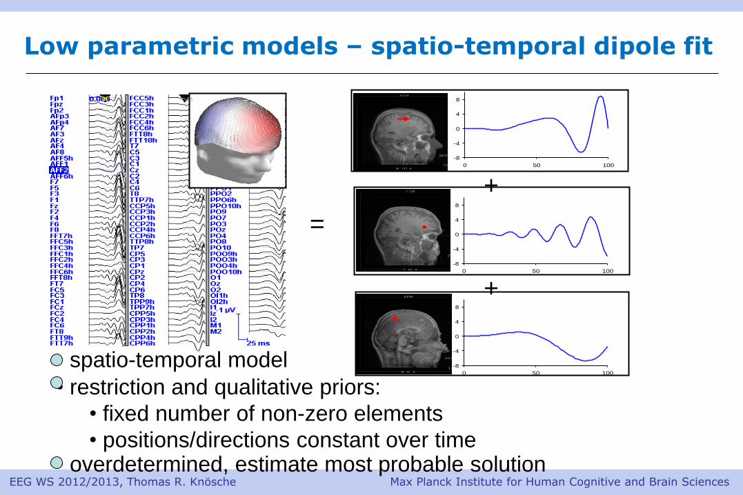
Low parametric models – spatio-temporal dipole fit C1
-8
-4
0
4
8
0 50 100
C2
-8
-4
0
4
8
0 50 100
C3
-8
-4
0
4
8
0 50 100
=
+
+
• spatio-temporal model
• restriction and qualitative priors:
• fixed number of non-zero elements
• positions/directions constant over time • overdetermined, estimate most probable solution

EEG WS 2012/2013, Thomas R. Knösche Max Planck Institute for Human Cognitive and Brain Sciences
Distributed sources – cortical current density imaging
=
• spatial model
• restriction and qualitative priors:
• activity only in cortex with perpendicular direction
• minimum norm (e.g. L2, L1, LORETA) • estimate most probable solution
Dale et al. (Neuron 2000); Liu et al. (Proc. Nat. Acad. Sci. USA 1998)
EEG WS 2012/2013, Thomas R. Knösche Max Planck Institute for Human Cognitive and Brain Sciences
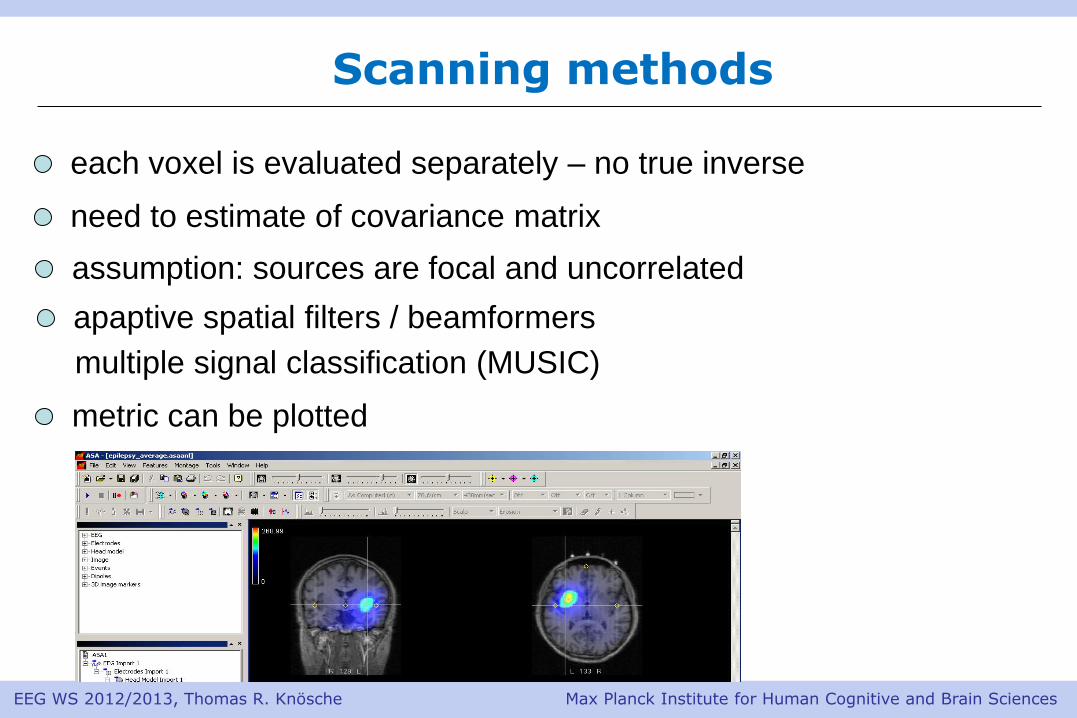
Scanning methods
each voxel is evaluated separately – no true inverse
need to estimate of covariance matrix
assumption: sources are focal and uncorrelated
apaptive spatial filters / beamformers
multiple signal classification (MUSIC)
metric can be plotted
EEG WS 2012/2013, Thomas R. Knösche Max Planck Institute for Human Cognitive and Brain Sciences
Take home messages
The inverse problem is non-unique. There is a multi-dimensional
manifold of solutions with equal maximum probability conditional
upon the measurements.
Every solution is equally valid conditional upon the data and the
priors.
Scanning methods are no true inverse solutions. Yet, they yield
much useful information on the sources.
Due to noise and errors, we cannot determine solutions with certaintly.
This is expressed by posterior distributions. However, mostly we
estimate the most probable solution.
We need priors. Priors can encode source space restrictions,
general qualitative properties or explicit quantitative knowledge.

EEG WS 2012/2013, Thomas R. Knösche Max Planck Institute for Human Cognitive and Brain Sciences
Take home messages

EEG WS 2012/2013, Thomas R. Knösche Max Planck Institute for Human Cognitive and Brain Sciences
Thank you
Thank you