INTERNATIONAL JOURNAL OF · PDF fileDickson Siele Cheruiyot [email protected] ... Egerton...

INTERNATIONAL JOURNAL OF SCIENTIFIC AND STATISTICAL COMPUTING (IJSSC)

VOLUME 5, ISSUE 1, 2014

EDITED BY

DR. NABEEL TAHIR

ISSN (Online): 2180-1339

International Journal of Scientific and Statistical Computing (IJSSC) is published both in

traditional paper form and in Internet. This journal is published at the website

http://www.cscjournals.org, maintained by Computer Science Journals (CSC Journals), Malaysia.

IJSSC Journal is a part of CSC Publishers

Computer Science Journals

http://www.cscjournals.org

INTERNATIONAL JOURNAL OF SCIENTIFIC AND STATISTICAL

COMPUTING (IJSSC)

Book: Volume 5, Issue 1, January / February 2014

Publishing Date: 11-02-2014

ISSN (Online): 2180 -1339

This work is subjected to copyright. All rights are reserved whether the whole or

part of the material is concerned, specifically the rights of translation, reprinting,

re-use of illusions, recitation, broadcasting, reproduction on microfilms or in any

other way, and storage in data banks. Duplication of this publication of parts

thereof is permitted only under the provision of the copyright law 1965, in its

current version, and permission of use must always be obtained from CSC

Publishers.

IJSSC Journal is a part of CSC Publishers

http://www.cscjournals.org

© IJSSC Journal

Published in Malaysia

Typesetting: Camera-ready by author, data conversation by CSC Publishing Services – CSC Journals,

Malaysia

CSC Publishers, 2014

EDITORIAL PREFACE

The International Journal of Scientific and Statistical Computing (IJSSC) is an effective medium for interchange of high quality theoretical and applied research in Scientific and Statistical Computing from theoretical research to application development. This is the First Issue of Fifth Volume of IJSSC. International Journal of Scientific and Statistical Computing (IJSSC) aims to publish research articles on numerical methods and techniques for scientific and statistical computation. IJSSC publish original and high-quality articles that recognize statistical modeling as the general framework for the application of statistical ideas.

The initial efforts helped to shape the editorial policy and to sharpen the focus of the journal. Started with Volume 5, 2014, IJSSC appears with more focused issues. Besides normal publications, IJSSC intend to organized special issues on more focused topics. Each special issue will have a designated editor (editors) – either member of the editorial board or another recognized specialist in the respective field.

This journal publishes new dissertations and state of the art research to target its readership that not only includes researchers, industrialists and scientist but also advanced students and practitioners. The aim of IJSSC is to publish research which is not only technically proficient, but contains innovation or information for our international readers. In order to position IJSSC as one of the top International journal in computer science and security, a group of highly valuable and senior International scholars are serving its Editorial Board who ensures that each issue must publish qualitative research articles from International research communities relevant to Computer science and security fields.

IJSSC editors understand that how much it is important for authors and researchers to have their work published with a minimum delay after submission of their papers. They also strongly believe that the direct communication between the editors and authors are important for the welfare, quality and wellbeing of the Journal and its readers. Therefore, all activities from paper submission to paper publication are controlled through electronic systems that include electronic submission, editorial panel and review system that ensures rapid decision with least delays in the publication processes. To build international reputation of IJSSC, we are disseminating the publication information through Google Books, Google Scholar, Directory of Open Access Journals (DOAJ), Open J Gate, ScientificCommons, Docstoc, Scribd, CiteSeerX and many more. Our International Editors are working on establishing ISI listing and a good impact factor for IJSSC. I would like to remind you that the success of the journal depends directly on the number of quality articles submitted for review. Accordingly, I would like to request your participation by submitting quality manuscripts for review and encouraging your colleagues to submit quality manuscripts for review. One of the great benefits that IJSSC editors provide to the prospective authors is the mentoring nature of the review process. IJSSC provides authors with high quality, helpful reviews that are shaped to assist authors in improving their manuscripts.

EDITORIAL BOARD Associate Editor-in-Chief (AEiC) Dr Hossein Hassani Cardiff University United Kingdom EDITORIAL BOARD MEMBERS (EBMs) Dr. De Ting Wu Morehouse College United States of America Dr Mamode Khan University of Mauritius Mauritius Dr Costas Leon César Ritz College Switzerland

Assistant Professor Christina Beneki Technological Educational Institute of Ionian Islands Greece

Professor Abdol Soofi University of Wisconsin-Platteville United States of America Assistant Professor Yang Cao Virginia Tech United States of America

International Journal of Scientific and Statistical Computing (IJSSC), Volume (5) : Issue (1) : 2014

TABLE OF CONTENTS

Volume 5, Issue 1, January / February 2014

Pages

1 - 14

Distribution of Nairobi Stock Exchange 20 Share Index Returns: 1998-2011

Cox Lwaka Tamba, Dickson Siele Cheruiyot, Martin Wafula Nandelenga

15 - 23

Probabilistic Analysis of a Desalination Plant with Major and Minor Failures and Shutdown

During Winter Season

Padmavathi N, S. M. Rizwan, Anita Pal, Gulshan Taneja

Cox Lwaka Tamba, Dickson Siele Cheruiyot & Martin Wafula Nandelenga

International Journal of Scientific and Statistical Computing (IJSSC), Volume (5) : Issue (1) : 2014 1

Distribution of Nairobi Stock Exchange 20 Share Index Returns: 1998-2011

Cox Lwaka Tamba [email protected] Faculty of Science/Department of Mathematics Division of Statistics Egerton University P.o. Box 536-20115, Egerton, Kenya

Dickson Siele Cheruiyot [email protected] Faculty of Science/Department of Mathematics Division of Statistics Egerton University P.o. Box 536-20115, Egerton, Kenya

Martin Wafula Nandelenga [email protected] Faculty of Arts and Social Sciences Department of Economics Egerton University P.o. Box 536, Egerton, Kenya

Abstract

The assumption that returns of daily share index prices are normally distributed has long been disputed by the data. In this paper, the normality assumption has been tested using time series data of daily Nairobi Stock Exchange 20-Share Index (NSE 20-Share Index) for the period 1998-2011. It has been confirmed that the share price index returns does not follow the normal distribution. Other symmetrical distributions have been fit to the data i.e. logistic distribution and t- location scale distribution. With the aid of a programming language; Matlab we have computed the various Maximum Likelihood (ML) estimates from this distributions and tested how well they fit to the data. It has been established that the NSE 20 Share Index returns follows a t-location scale distribution (normal inverse gamma mixture). We recommend that since we have found that the normal inverse gamma mixture best fits the NSE 20 Share Index return, other normal mixtures can be investigated how well they fit this data.

Keywords: Returns, Leptokurtosis, Tail, 20 Share Index, t-location Scale.

1. INTRODUCTION A stock market index is a measure of changes in the stocks markets and is usually considered to be a reasonably representative of the market as a whole. Indexes are usually tabulated on a daily basis and involve summarizing sample share price movements (NSE 20 share index) or all the share prices movements (NSE All Share Index, (NASI)). The NSE 20 Share index measures the average performance of 20 large cap stocks drawn from different industries. Stock prices and returns have been assumed to be normally distributed.

The first complete development of a theory of random walks in security prices is due to Bachelier (1900), whose original work first appeared around the turn of the century. Unfortunately his work did not receive much attention from economists. The Bachelier (1900) model assumed that under the central-limit theorem the daily, weekly, and monthly price changes will each have normal or Gaussian distributions. However it has been found out that most of the distributions of price changes are leptokurtic; that is, there are too many values near the mean and too many out in the extreme tails.



Mandelbrot (1962) asserts that, in the past, academic research has too readily neglected the implications of the leptokurtosis usually observed in empirical distributions of price changes. Mandelbrot (1963) studied the stable Paretian distribution and showed that it is the distribution of price changes provided the characteristic exponent is less than two.

Fama (1965) discussed first in more detail the theory underlying the random-walk model and then tested the model's empirical validity. The past behaviour of a security's price is rich in information concerning its future behaviour (Fama, 1965). The theory of random walk shows that the successive price changes are independent, identically distributed random variables. Most simply this implies that the series of price changes has no memory, that is, the past cannot be used to predict the future in any meaningful way. The probability distribution of the price changes during time period t is independent of the sequence of price changes during the previous time periods i.e,

1 1Pr s|S , s , . . . Pr st t t tS S (1)

The actual tests were not performed on the daily prices themselves but on the first differences of their natural logarithms. The variable of interest was

1 1log logt e t e tu S S , (2)

where1tS is the price of the security at the end of day t+1.

Fama (1965) demonstrated that first differences of stock prices seem to follow stable Paretian distributions with characteristic exponent is less than two.

According to Officer, (1972), the distribution of stock returns has some characteristics of a non-normal generating process i.e. the results indicate the distribution is "fat- tailed" relative to a normal distribution. However, characteristics were also observed which are inconsistent with a stable non-normal generating process. Evidence is presented illustrating a tendency for longitudinal sums of daily stock returns to become "thinner-tailed" for larger sums, but not to the extent that a normal distribution approximates the distribution. This confirms that the normal distribution is not a good fit for the distribution of stock and index prices.

Praetz (1972) presented both theoretical and empirical evidence about a probability distribution which describes the behaviour of share price changes. Osborne's Brownian motion theory of share price changes was modified to account for the changing variance of the share market. This produced a scaled t-distribution which is an excellent fit to series of share price indices. This distribution was the only known simple distribution to fit changes in share prices. It provided a far better fit to the data than the stable Paretian, compound process, and normal distributions (Praetz, 1972).

The Student and symmetric-stable distributions, as models for daily rates of return on common stocks, have been discussed and empirically evaluated (Blattberg, 1974). Both models were derived using the framework of subordinated stochastic processes. Some important theoretical and empirical implications of these models were also discussed. The descriptive validity of each model, relative to the other, was assessed by applying each model to actual daily rates of return. Interpretations of empirical results were guided by results from a Monte Carlo investigation of the properties of estimators and model-comparison methods. The major inference of this report was that, for daily rates of return, the Student model has greater descriptive validity than the symmetric-stable model.

Hung et al, (2007) studied the variation of Taiwan stock market using the statistical methods developed by econophysicists. The Taiwan market was found to have a fat tail as found in the markets of other countries, but it did not follow a power law as the others. The cumulative



distribution of daily returns in Taiwan stock index could be fitted quite well using the log-normal

distribution, and even better by a power law with an exponential cut-off. They believed that the distinct behaviour of Taiwan market was mainly due to the protective measures taken by the government.

Barndorff, (1977) introduced a family of continuous type distributions such that the logarithm of the probability (density) function is a hyperbola (or, in several dimensions, a hyperboloid). The focus was on the mass-size distribution of aeolian sand deposits however, this distribution has been widely used to model stock returns. Barndorff (1978) discussed the generalised hyperbolic distributions which includes the hyperbolic distributions and some distributions which induce distributions on hyperbolae or hyperboloids analogous to the von Mises-Fisher distributions on spheres. It is, among other things, shown that distributions of this kind are a mixture of normal distributions. Eberlin (1995) based on a data set consisting of the daily prices of the 30 DAX share over three years period, investigated the distributional form of compound returns. A class of hyperbolic distribution was fit to the empirical returns with high accuracy. Hyperbolic distributions fit empirical return adequately, (Kuchler et al. (1999) and Bibby (2003)).

The logistic distribution is a general stochastic measurement model; it has been used in measuring risk incurred in financial assets returns, (Osu, 2010). It has been observed that the initial stage of growth of the worth of a business enterprise is approximately exponential. At a time the growth slows down. Osu, 2010 asserts that this could be due to diversification (investing in more than one stock), since the returns on different stocks do not move exactly in the way all the time. Ultimately the growth of the firm is stable and it may not be affected by risk since diversification reduces risk.

Stock returns turn out to be quite sensitive to the degree to which distributions are thick tailed and asymmetric. Lack of encoding information about asymmetry and leptokurtosis is a well-known drawback of the Normal distribution. This has led to a search for alternative distributions. In this work, we test the normality assumption on the NSE 20 Share Price Index. We also fit the logistic and the t- location scale distribution to find the best fit to this data.

2. MODELS OF NSE 20 SHARE INDEX RETURNS In this section we present the distributions used in this study. The normal distribution is fully discussed in Section 2.1. Section 2.2 presents the logistic distribution whereas the t- location scale is presented in Section 2.3. In all this sections, we review the construction, properties and estimation of these distributions. It is important to mention that from this point onwards, the sample herein referred to consists of the NSE 20 Share Index for the year 1998 to 2011. These indices are published daily in the Kenya local newspapers. The series analyzed, is the series of returns, where returns are defined as,

1100 log logt t tR S S . (3)

The behavior of the NSE 20 Share Index considered during this period is shown below in Figure

1. The series analyzed for each market is the series of returns, where returns are defined as,



given in Equation (3).

0 500 1000 1500 2000 2500 3000 3500-6

-4

-2

0

2

4

6

8

10

Return %

Relat

ive F

requ

ency

RETURNS OF NSE 20 SHARE INDEX

FIGURE 1: Percentage Returns, Rt of NSE 20 Share Index.

where tR and

tS are the return and the index in day t, respectively. The histogram of this data is

shown below;

-4 -2 0 2 4 6 80

0.1

0.2

0.3

0.4

0.5

0.6

0.7

Data

Dens

ity

Rt data

FIGURE 2: A Histogram of Returns Rt of NSE 20 Share Index.

Table 1 below summarizes some relevant information about the empirical distributions of stock returns under consideration. The statistics reported are the mean, standard deviation, minimum and maximum return during the sample period, coefficients of skewness and kurtosis.

Mean Variance Minimum Value

Maximum Value

Skewness Kurtosis

47.9454 10 0.7881 -5.2339 9.1782 0.5970 13.1608

TABLE 1: Sample Moments of the Distributions NSE 20 Share Index.



The third central moment is often called a measure of asymmetry or skewness in the distribution. From our descriptive results shown above, the distribution of this data is approximately symmetrical though it shows signs of being positively skewed. The coefficient of skewness is almost 0.5970. This is well depicted from the histogram in Figure 2 above.

Kurtosis measures a different type of departure from normality by indicating the extent of the peak (or the degree of flatness near its center) in a distribution. We see that this is the ratio of the fourth central moment divided by the square of the variance. If the distribution is normal, then this ratio is equal to 3. A ratio greater than 3 indicates more values in the neighborhood of the mean (is more peaked than the normal distribution). Our data has a fat tail or excess kurtosis as shown in the coefficient of kurtosis (i.e. kurtosis of 13.1608). The distribution of this data is leptokurtic.

2.1 Normality Assumption Test

A random variable is said to be normal distributed with mean, and variance, 2 (Mood, 2001)

if its probability distribution is

2

22

1( ) exp , , 0.

22

i

i

t

t t

rf r for r

(4)

The maximum likelihood estimates of the normal distribution with their corresponding standard errors are shown below in Table 2 below;

Parameter Estimate Std error

0.000794536 0.0151517

0.887763 0.0107162

TABLE 2: ML Estimates of the Normal Distribution.

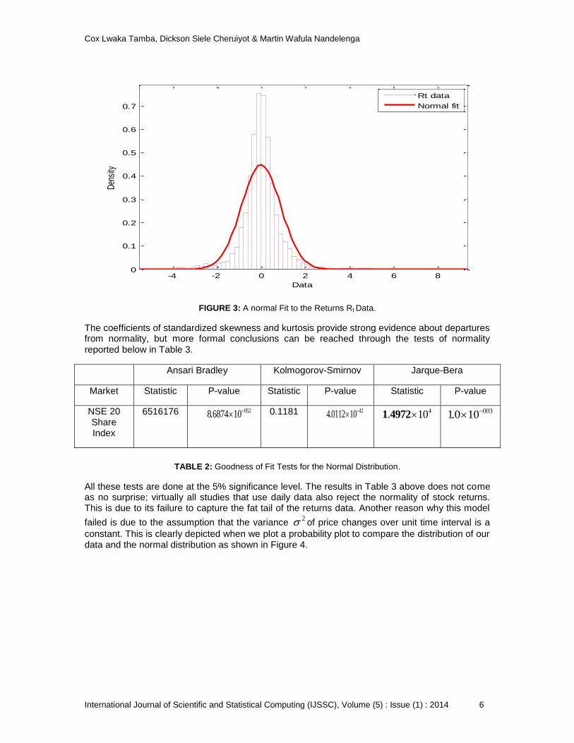
The distribution of financial returns over horizons shorter than a month is not well described by a normal distribution. In particular, the empirical return distributions, while unimodal and approximately symmetric, are typically found to exhibit considerable leptokurtosis. The typical shape of the return distribution, as compared to a fitted normal is presented in Figure 3 below.



-4 -2 0 2 4 6 80

0.1

0.2

0.3

0.4

0.5

0.6

0.7

Data

Den

sity

Rt data

Normal fit

FIGURE 3: A normal Fit to the Returns Rt Data.

The coefficients of standardized skewness and kurtosis provide strong evidence about departures from normality, but more formal conclusions can be reached through the tests of normality reported below in Table 3.

Ansari Bradley Kolmogorov-Smirnov Jarque-Bera

Market Statistic P-value Statistic P-value Statistic P-value

NSE 20 Share Index

6516176

052 8.6874 10 0.1181 42 4.0112 10

4. 101 4972 0031.0 10

TABLE 2: Goodness of Fit Tests for the Normal Distribution.

All these tests are done at the 5% significance level. The results in Table 3 above does not come as no surprise; virtually all studies that use daily data also reject the normality of stock returns. This is due to its failure to capture the fat tail of the returns data. Another reason why this model

failed is due to the assumption that the variance 2 of price changes over unit time interval is a

constant. This is clearly depicted when we plot a probability plot to compare the distribution of our data and the normal distribution as shown in Figure 4.



-4 -2 0 2 4 6 8

0.00010.00050.0010.0050.010.050.1

0.250.5

0.750.9

0.950.990.995

0.9990.99950.9999

Data

Pro

babi

lity

Rt data

normal fit

FIGURE 4: A Probability Plot of the Normal Fit.

The goodness of fit coupled with the probability plot give a clear evidence against the normal distribution as a fit of the Returns of NSE 20 Share Price Index. In order to test what specification describes the data better than the Normal distribution, we consider in the next part two alternative distributions that allow for the characteristics of the data discussed above; we then fit such distributions to the data in the following part.

2.2 Fitting a Logistic Distribution The density function of the logistic distribution is given by

2

exp

( | , ) ,

1 exp

i

i i

i

t

t t

t

r

f r for r

r

(5)

where µ (-∞ < µ < ∞) is a location parameter and ( >0) is a dispersion (or scale) parameter.

(Walck, 2007). This distribution, which is very similar to the normal in that it is symmetric but has thicker tails, and it has been first suggested as appropriate to model stock return. The maximum likelihood estimates of this distribution are obtained using the Expectation Maximization (EM) algorithm.

Parameter Estimate Std error

-0.00461803 0.0121681

0.423535 0.00620854

TABLE 4: ML Estimates for the Logistic Distribution.



The estimates in Table 4 above are used to fit the logistic distribution to the returns NSE 20 Share Index data. The shape of the return distribution, as compared to a fitted logistic distribution is presented in Figure 4 below.

-4 -2 0 2 4 6 80

0.1

0.2

0.3

0.4

0.5

0.6

0.7

Data

Den

sity

Rt data

logistic fit

FIGURE 5: A logistic Distribution Fit to the Returns Rt Data.

Tests of goodness of fit results at 5% level of significance are presented in Table 5 below;

Ansari Bradley Kolmogorov-Smirnov

Market Statistic P-value Statistic P-value

NSE 20 Share Index

6155059 0102.2026 10 0.0460 0.0013

TABLE 5: Goodness of Fit Tests for the Logistic Distribution.

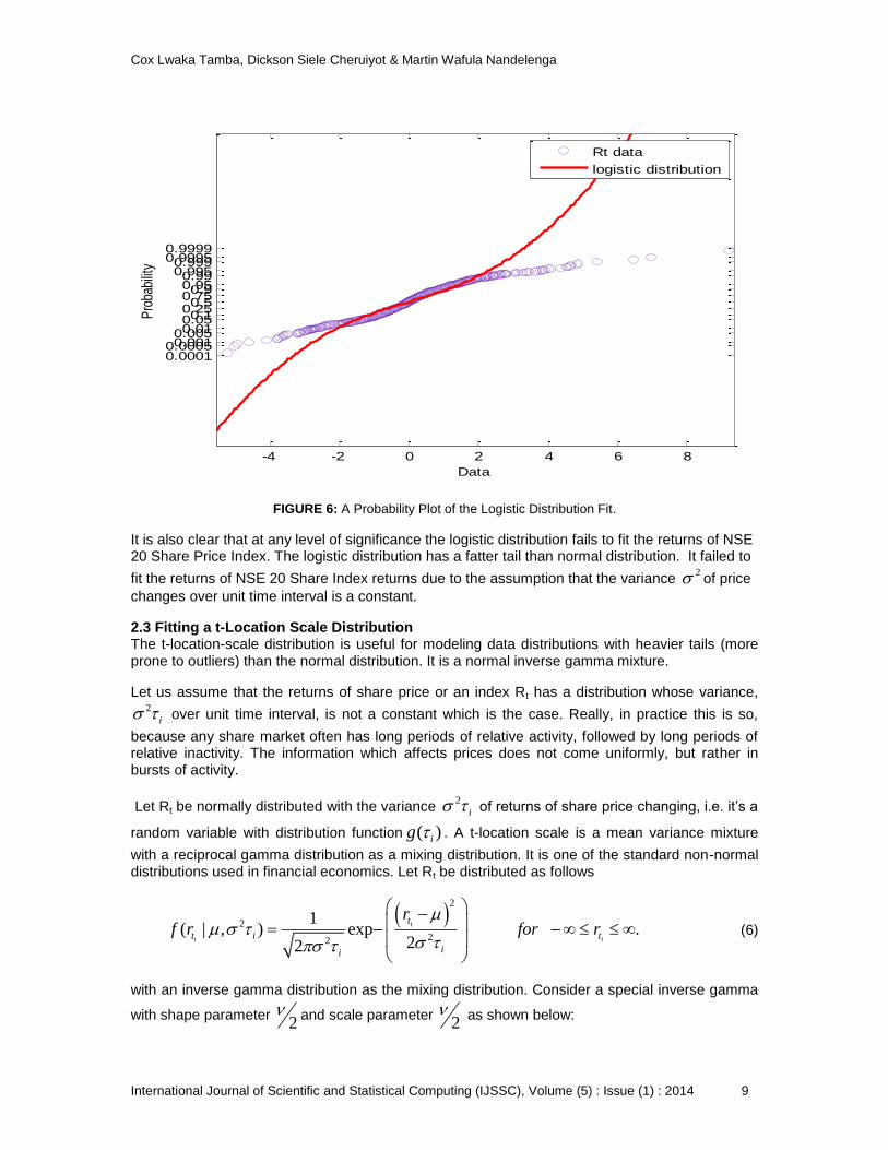
The probability plot of the distribution of our data and the logistic distribution is represented in Figure 6 below;



-4 -2 0 2 4 6 8

0.00010.00050.0010.0050.010.050.10.250.5

0.750.90.95

0.990.9950.9990.9995

0.9999

Data

P

roba

bilit

yRt data

logistic distribution

FIGURE 6: A Probability Plot of the Logistic Distribution Fit.

It is also clear that at any level of significance the logistic distribution fails to fit the returns of NSE 20 Share Price Index. The logistic distribution has a fatter tail than normal distribution. It failed to

fit the returns of NSE 20 Share Index returns due to the assumption that the variance 2 of price

changes over unit time interval is a constant.

2.3 Fitting a t-Location Scale Distribution The t-location-scale distribution is useful for modeling data distributions with heavier tails (more prone to outliers) than the normal distribution. It is a normal inverse gamma mixture.

Let us assume that the returns of share price or an index Rt has a distribution whose variance, 2

i over unit time interval, is not a constant which is the case. Really, in practice this is so,

because any share market often has long periods of relative activity, followed by long periods of relative inactivity. The information which affects prices does not come uniformly, but rather in bursts of activity.

Let Rt be normally distributed with the variance 2

i of returns of share price changing, i.e. it’s a

random variable with distribution function ( )ig . A t-location scale is a mean variance mixture

with a reciprocal gamma distribution as a mixing distribution. It is one of the standard non-normal distributions used in financial economics. Let Rt be distributed as follows

2

2

22

1( | , ) exp .

22

i

i i

t

t i t

ii

rf r for r

(6)

with an inverse gamma distribution as the mixing distribution. Consider a special inverse gamma

with shape parameter 2

and scale parameter 2

as shown below:



(7)

and so the distribution,

2 2

0

, , , ,i it t i i if r f r g d

(8)

which simplifies to,

1

2 2

2

2

11

12, , , , , 0

2

i

i i

t

t t

r

f r for r R

(9)

This is a t- location scale distribution as shown by (Barndorff, 1988). If a random variable Rt has a

t- location with parameters , and then the random variable tr

has a student t-

distribution with degrees of freedom. The mean, variance and kurtosis for this distribution are

,

2

2

and

3( 2)

4

respectively (Wenbo, 2006).

Using the Expectation Maximization algorithms of the t- location scale distribution, we obtain the maximum likelihood estimates of the t- location scale distribution.

Parameter Estimate Std. Error

-0.00889354 0.0102819

0.480765 0.0115711

2.42046 0.124132

TABLE 6: ML Estimates for the t-location Scale Distribution.

Using these estimates we fit the t-location scale distribution to the NSE 20 Share Index data. The shape of the return distribution, as compared to a fitted t-location scale distribution is presented in Figure 7 below.

2

1 222

2

i

i ig e



-4 -2 0 2 4 6 80

0.1

0.2

0.3

0.4

0.5

0.6

0.7

Data

Density

Rt data

t- location scale fit

FIGURE 7: A t- location Scale Distribution fit to the Returns Rt Data.

Tests of goodness of fit results at 5% level of significance are presented in Table 7 below;

Ansari Bradley Kolmogorov-Smirnov

Market Statistic P-value Statistic P-value

NSE 20 Share Index

5922916 0.4883 0.0192 0.5460

TABLE 7: Goodness of Fit Tests for the t-location Scale Distribution.

The probability plot of the return distribution and the t-location scale distribution is given Figure (8) below;



-4 -2 0 2 4 6 8

0.0001

0.00050.001

0.0050.01

0.05

0.1

0.25

0.5

0.75

0.9

0.95

0.990.995

0.9990.9995

0.9999

Data

Pro

babili

ty

Rt data

t-location scale fit

FIGURE 8: A Probability Plot of the t-location Scale Distribution Fit.

We have found strong support for the t-location scale distribution, which cannot be rejected at any reasonable significance level. This is because the t- location scale captures the fat tail exhibited in the NSE 20 Share Index returns. This also provides a clear evidence of the fact that the variance of price changes over unit time interval is a not constant. This is the case in practice because any share market often has long periods of relative activity, followed by long periods of relative inactivity. The information which affects prices does not come uniformly, but rather in

bursts of activity. This is a formal evidence of the fact 2 varies significantly from year to year, as

the degree of activity in the market also varies. Having established that the t-location scale (rather than the Normal) distribution properly describes daily NSE 20 Share Index, we conclude any predictions on the returns of NSE 20 Share Index should be based on the t-location scale distribution and not the normal distribution. Studies in financial economics can be based on the t- location scale distribution.

3. CONCLUSION This study was interested in fitting an empirical distribution to the NSE 20 share index. In finding returns we used changes in logarithms prices instead of simple price changes. This is because; i) The change in log price is the yield, with continuous compounding, from holding the security for that day. ii) It has been shown that the variability of simple price changes for a given stock is an increasing function of the price level of the stock. Taking logarithms seems to neutralize most of this price level effect.



iii) For changes less than 15 percent, the change in log price is very close to the percentage price change, and for many purposes it is convenient to look at the data in terms of percentage price changes.

After thorough descriptive analysis it was clear that the NSE 20 share price index data is approximately symmetrical though it shows signs of being positively skewed. The coefficient of skewness is almost 0.5970. The data also exhibited a fat tail or excess kurtosis hence leptokurtic (i.e. kurtosis of 13.1608).

In an attempt to fit a normal distribution to the NSE 20 share price index data all tests done at the 5% significance level led to rejection of this distribution. This is due to the fact that the normal distribution fails to capture the fat tail of the returns data. Another reason why this model failed is

due to the assumption that the variance 2 of price changes over unit time interval is a constant.

Though the logistic distribution has a fatter tail than normal distribution, it was also rejected at 5% level of significance. It failed to fit the returns of NSE 20 Share Index returns due to the

assumption that the variance 2 of price changes over unit time interval is a constant.

The t-location scale distribution has a fatter tail than the normal and logistic distributions. In the construction of this distribution, the scale parameter (i.e. the variance) is not assumed constant. From our results, we found strong support for the t-location scale distribution, which could not be rejected at any reasonable significance level. This is because it captures the fat tail exhibited in the NSE 20 Share Index returns. This also provides a clear evidence of the fact that the variance

of price changes over unit time interval is not a constant. This is a formal evidence of the fact 2

varies significantly from year to year, as the degree of activity in the market also varies. From these results, we conclude that any predictions on the returns of NSE 20 Share Index should be based on the t-location scale distribution and not the normal distribution. Studies in financial economics could be based on the t- location scale distribution. We further recommend that since we have found that the normal inverse gamma mixture best fits the NSE 20 Share Index return, other normal mixtures can be investigated how well they fit this data.

4. REFERENCES

[1] A. M. Mood, F.A. Graybill, and C. D. Boes. “An Introduction to the Theory of Statistics”. Tata McGraw Publishing Company Limited 2001, pp 107.

[2] B. Mandelbrot. "The Variation of Certain Speculative Prices," Journal of Business, 394-419 October 1963.

[3] B. Mandelbrot. “Paretian Distributions and Income Maximization”. The Quarterly Journal of Economics, Vol. 76, No. 1., pp. 57-85 Feb., 1962.

[4] C. Blattberg C., and N. J. Gonedes. “A Comparison of the Stable and Student Distributions as Statistical Models for Stock Prices”. Source: The Journal of Business, Vol. 47, No. 2, pp. 244-280. Apr., 1974.

[5] C. Hung, and S. Liaw.). “Statistical properties of Taiwan Stock Index”. Department of Physics, National Chung-Hsing University, 250 Guo-Kuang Road, Taichung, Taiwan Jan 9, 2007.

[6] C. Walck. “Handbook on Statistical Distributions for Experimentalists”.. University of Stockholm, Particle Physics Group. 2007, pp 84.

[7] F. Aparicio, and J. Estrada. “Empirical Distributions of Stock Returns: Scandinavian Securities Markets”. (1990-95).



[8] F. E. Fama. “The Behavior of Stock-Market Prices”. The Journal of Business, Vol. 38, No. 1., pp. 34-105 Jan., 1965.

[9] H. Wenbo, N. K. Alec. “The Skewed t-distribution for Portfolio Credit Risk”. Florida State University, 2006.

[10] L. Bachelier. “In the random character of stock market prices” (edited by P.H Cootner), Theorie de la speculation, Gauthiers, MA, (1964) Paris Cambridge; pp 17-18, 1900.

[11] M. Bibby. “Hyperbolic Processes in Finance”. Institute of Mathematics and Physics, The Royal Veterinary and Agricultural University Thorvaldsensvej 40 DK-1871 Frederiksberg C, DenmarkMichael Sørensen Department of Statistics and Operations Research Institute of Mathematical Sciences University of Copenhagen Universitetsparken 5 DK-2100 København Ø, Denmark, 2003.

[12] O. B. Osu. “Application of the logistic function to the Assessment of the Risk of Financial Assets Returns”. Journal of Modern Mathematics and Statistics, 4 (1) 7-10, 2010.

[13] O. Barndorff-Nielsen. “Exponentially Decreasing Distributions for the Logarithm of Particle Size”. Source: Proceedings of the Royal Society of London. Series A, Mathematical and Physical Sciences, Vol. 353, No. 1674, pp. 401-419, Mar. 25, 1977.

[14] O. Barndorff-Nielsen. “Hyperbolic Distributions and Distributions on Hyperbolae”. Source: Scandinavian Journal of Statistics, Vol. 5, No. 3, pp. 151-157 Published by: Wiley on behalf of Board of the Foundation of the Scandinavian Journal of Statistics,1978.

[15] O. Barndorff-Nielsen. Processes of normal inverse Gaussian type. Finance Stoch 2:41–68, 1988.

[16] P. D. Praetz. “The Distribution of Share Price Changes”. Source: The Journal of Business, Vol. 45, No. 1, pp. 49-55 Published by: The University of Chicago Press Jan., 1972.

[17] R. R. Officer. “The Distribution of Stock Returns”: R. R. Source: Journal of the American Statistical Association, Vol. 67, No. 340, pp. 807- 812 ,Dec., 1972.

[18] U. Keller. “Hyperbolic distributions in finance”- Ernst eberlin 1995.

Padmavathi N, S. M. Rizwan, Anita Pal & Gulshan Taneja

International Journal of Scientific and Statistical Computing (IJSSC), Volume (5) : Issue (1):2014 15

Probabilistic Analysis of a Desalination Plant with Major and Minor Failures and Shutdown During Winter Season

Padmavathi N [email protected] Department of Mathematics & Statistics Caledonian college of Engineering Muscat, Sultanate of Oman

S. M. Rizwan [email protected] Department of Mathematics & Statistics Caledonian college of Engineering Muscat, Sultanate of Oman

Anita Pal [email protected] Department of Mathematics National Institute of Technology Durgapur, India

Gulshan Taneja [email protected] Department of Statistics M D University Rohtak, India

Abstract In many desalination plants, multi stage flash desalination process is normally used for sea water purification. The probabilistic analysis and profitability of such a complex system with standby support mechanism is of great importance to avoid huge loses. Thus, the aim of this paper is to present a probabilistic analysis of evaporators of a desalination plant with major and minor failure categories and estimating various reliability indicators. The desalination plant operates round the clock and during the normal operation; six of the seven evaporators are in operation for water production while one evaporator is always under scheduled maintenance and used as standby. The complete plant is shut down for about one month during winter season for annual maintenance. The water supply during shutdown period is maintained through ground water and storage system. Any major failure or annual maintenance brings the evaporator/plant to a complete halt and appropriate repair or maintenance is undertaken. Measures of plant effectiveness such as mean time to system failure, availability, expected busy period for maintenance, expected busy period for repair, expected busy period during shutdown & expected number of repairs are obtained by using semi-Markov processes and regenerative point techniques. Profit incurred to the system is also evaluated. Seven years real data from a desalination plant are used in this analysis. Keywords: Desalination Plant, Minor/Major Failures, Repairs, Semi – Markov, Regenerative Process.

1. NOTATIONS

O Operative state of evaporator

U�� Under Maintenance during summer



U�� Under Maintenance during winter before service

U�� Under Maintenance during winter after service

U�� Under Maintenance during summer before service

F� Failed unit is under minor repair during summer

F�� Failed state of the evaporator due to minor repair during summer

F� Failed unit is under major repair during summer

F� � Failed state of the evaporator due to major repair during summer

F�� Failed unit is under minor repair during winter before service

F�� Failed state of the evaporator due to minor repair during winter before service

F� �� Failed unit is under major repair during winter before service

F� �� Failed state of the evaporator due to major repair during winter before service

F�� Failed unit is under minor repair during winter after service

F�� Failed state of the evaporator due to minor repair during winter after service

F� �� Failed unit is under major repair during winter after service

F� �� Failed state of the evaporator due to major repair during winter after service

F Failed state of one of the evaporator

β1 Rate of the unit moving from summer to winter

β2 Rate of the unit moving from winter to summer

λ Rate of failure of any component of the unit

γ Maintenance rate

γ1 Rate of shutting down

γ2 Rate of recovery after shut down during winter

α1 Repair rate for minor repairs

α2 Repair rate for major repairs

λ1 Maintenance rate including the rate of inspection

p1 Probability of occurrence of minor repair



p2 Probability of occurrence of major repair

©

Symbol for Laplace convolution

Symbol for Stieltje’s convolution

* Symbol for Laplace Transforms

** Symbol for Laplace Stieltje’s Transforms

C0 Revenue per unit uptime

C1 Cost per unit uptime for which the repairman is busy for maintenance

C2 Cost per unit uptime for which the repairman is busy for repair

C3 Cost per unit uptime for which the repairman is busy during shutdown

C4 Cost per unit repair require replacement (all costs are taken in Rial Omani i.e., RO)

A0 Steady state availability of the system

�� Expected busy period of the repairman during maintenance

�� Expected busy period of the repairman for repair

�� Expected busy period of the repairman during shutdown

�� Expected number of repairs require replacement

∅�(�)

c.d.f. of first passage time from a regenerative state i to a failed state j

qij(t), Qij(t)

p.d.f. and c.d.f. of first passage time from a regenerative state i to a regenerative state

j or to a failed state j in (0, t]

gm(t), Gm(t) p.d.f. and c.d.f. of maintenance rate

gm1(t),Gm1(t) p.d.f. and c.d.f. of maintenance time including inspection

gs(t), Gs(t) p.d.f. and c.d.f. of shutdown rate

gr(t), Gr(t) p.d.f. and c.d.f. of recovery rate

g1(t), G1(t) p.d.f. and c.d.f. of repair rate for minor repairs

g2(t), G2(t) p.d.f. and c.d.f. of repair rate for major repairs

2. INTRODUCTION Desalination is a water treatment process that removes the salt from sea water or brackish water. It is the only option in arid regions, since the rainfall is marginal. In many desalination plants, multi stage flash desalination process is normally used for water purification which is very expensive and involves sophisticated systems. Since, desalination plants are designed to fulfil the requirement of water supply for a larger sector in arid regions, they are normally kept in



continuous production mode especially during summer except for emergency/forced/planned outages. It is therefore; very important that the efficiency and reliability of such a complex system is maintained in order to avoid big loses. Establishing the numerical results of various reliability indices are extremely helpful in understanding the significance of these failures/maintenances on plant performance and assesses the impact of these failures on the overall profitability of the plant. Many researchers have expended a great deal of efforts in analysing industrial systems to achieve the reliability results that are useful for effective equipment/plant maintenance. Bhupender and Taneja [1] analysed a PLC hot standby system based on master-slave concept and two types of repair facilities, and many such analyses could be seen in the references therein. Mathew et al. [2] have presented an analysis of an identical two-unit parallel continuous casting plant system. Padmavathi et al. [3] have presented an analysis of the evaporator 7 of a seven unit desalination plant which fails due to any one of the six types of failures with the concept of inspection. Padmavathi et al. [4] explored a possibility of analyzing a desalination plant with emergency shutdown/unit tripping and online repair. Recently, Rizwan et al. [5] analyzed the desalination plant under the situation where repair or maintenance being carried out on a first come first served basis. Padmavathi et al. [6] analyzed a desalination plant with shutdown during winter season under the condition that the priority is given to repair over maintenance. However, analysis in [5] & [6] could have been better and more realistic results could be obtained if failures are categorized as minor and major failures and the repairs could be undertaken accordingly as the time to repair minor failures is comparatively lesser than the time required for fixing major failures. Also, it is viable to inspect the unit in order to identify the type of the failure and deal with it accordingly. Thus, as a future direction of [5], a variation into the analysis is shown and hence this paper is an attempt to present a probabilistic analysis of the plant under minor and major failure categories including inspection for estimating various reliability indicators. Seven years failure data of a desalination plant in Oman have been used for this analysis. Component failure, maintenance, plant shutdown rates, and various maintenance costs involved are estimated from the data. The desalination plant operates round the clock and during the normal operation; six of the seven evaporators are in operation for water production while one evaporator is always under scheduled maintenance and used as standby evaporator. This ensures the continuous water production with minimum possible failures of the evaporators. The complete plant is shut down for about a month during winter season because of the low consumption of water for annual maintenance; the water supply during this period is maintained through ground water and storage system. The evaporator fails due to any one of the two types of failure viz., minor and major. Repairable and serviceable failures are categorised as minor failures, whereas the replaceable failures are categorised as major failures. Any major failure or annual maintenance brings the plant to a complete halt and goes under forced outage state. Using the data, following values of rates and various costs are estimated:

• Estimated rate of failure of any component of the unit (λ) = 0.00002714 per hour

• Estimated rate of the unit moving from summer to winter (β1) = 0.0002315 per hour

• Estimated rate of the unit moving from winter to summer (β2) =0.0002315 per hour

• Estimated rate of maintenance (γ) = 0.0014881

• Estimated rate of shutting down (γ1) = 0.000114155 per hour

• Estimated rate of recovery after shut down during winter (γ2) = 0.0013889 per hour

• Estimated value of failure rate including inspection (λ1) = 0.4013889 per hour

• Estimated value of repair rate of minor repairs (α1) = 0.099216 per hour

• Estimated value of repair rate of major repairs (α2) = 0.059701 per hour

• Probability of occurrence of minor repair (p1) = 0.7419

• Probability of occurrence of major repair (p2) = 0.2581

• The revenue per unit uptime (C0) = RO 596.7 per hour



• Cost per unit uptime for which the repairman is busy for maintenance (C1) = RO 0.0626 per hour

• The cost per unit uptime for which the repairman is busy for repair (C2) = RO 0.003 per hour

• Cost per unit uptime for which the repairman is busy during shutdown (C3) = RO 16.378 per hour

• The cost per unit repair require replacement (C4) = RO 13.246 per hour

The plant is analysed probabilistically by using semi-Markov processes and regenerative point techniques. Measures of plant effectiveness/reliability indicators such as the mean time to system failure, plant availability, expected busy period during maintenance, expected busy period during repair, expected busy period during shut down and the expected number of repairs are estimated numerically.

3. MODEL DESCRIPTION AND ASSUMPTIONS

• There are seven evaporators in the desalination plant, of which 6 operate at any given time and one evaporator is always under scheduled maintenance.

• Maintenance of no evaporator is done if the repair of some other evaporator is going on.

• The various states of the evaporator are categorized under summer (states 0, 2, 5, 7,11and 12), winter (states 1, 4, 8, 9, 13 and 14), complete shutdown for overhaul/major service (state 3), and after major service (states 6, 10, 15, 16, 17and 18).

• The plant goes into shutdown for annual maintenance during winter season for one month.

• On completion of maintenance/repair, the repairman inspects as to whether the unit has failed due to minor/major failure, before putting the repaired unit into operation.

• If a unit is failed in one season, it gets repaired in that season only.

• Not more than two units fail at a time.

• During the maintenance of one unit, more than one of the other units cannot get failed.

• All failure times are assumed to have exponential distribution with failure rate ( λ )

whereas the repair times have general distributions.

4. TRANSITION PROBABILITIES AND MEAN SOJOURN TIMES A state transition diagram showing the possible states of transition of the plant is shown in Fig. 1. The epochs of entry into states 0, 1, 2, 3, 4, 5, 6, 7, 8, 9, 10, 15 and 16 are regeneration points and hence these states are regenerative states. 11, 12, 13, 14, 17 and 18 are non-regenerative states. The transition probabilities are given by:

dQ�� = γe&('() *)+ ), dt, dQ�/ = β/ e&('() *), G�2222(t)dt, dQ�3 = 6λe&('() *), G�2222(t)dt, dQ// = γe&('() +)+ ), dt, dQ/6 = γ/ e&('() +), G�2222(t)dt, dQ/7 = 6λe&('() +), G�2222(t)dt, dQ37 = β/e& *, G�22222(t)dt, dQ38 = 9/e& *, g�(t)dt, dQ3; = 93e& *, g�(t)dt, dQ6' = γ3e& + , dt dQ76 = γ/e& +, G�22222(t)dt, dQ7< = 9/g�(t)e& +, dt, dQ7= = 93g�(t)e& +, dt, dQ8� = e&'(, g/(t)dt, dQ88

(//) = >6λe&'(, © 1 A9/g/(t)dt , dQ8;(//) = >6λe&'(, © 1 A93g/(t)dt ,

dQ'� = β3 e&('() * ), G�2222(t)dt, dQ'' = e&('() * ), g�(t), dQ',/� = 6λ e&('() * ), G�2222(t)dt, dQ;� = e&'(, g3(t)dt, dQ;8

(/3) = >6λe&'(, © 1 A9/g3(t)dt , dQ;;(/3) = >6λe&'(, © 1 A93g3(t)dt

dQ</ = e&('() +), g/(t)dt, dQ<6 = γ/e&('() +), G/222(t)dt, dQ<6

(/6) = >6λe&('() + ), © γ/e& +, AG/222(t)dt , dQ<<(/6) = >6λe&('() + ), © e& +, A9/g/(t)dt ,

dQ<=(/6) = >6λe&('() + ), © e& +, A93g/(t)dt ,

dQ=/ = e&('() +), g3(t)dt, dQ=6 = γ/e&('() +), G3222(t)dt, dQ=6

(/7) = >6λe&('() + ), © γ/e& +, AG3222(t)dt , dQ=<(/7) = >6λe&('() + ), © e& +, A9/g3(t)dt ,



FIGURE 1: State Transition Diagram.

dQ==(/7) = >6λe&('() + ), © e& +, A93g3(t)dt ,

dQ/�,3 = β3e& * , G�22222(t)dt, dQ/�,/8 = 9/e& * , g�(t)dt, dQ/�,/' = 93e& * , g�(t)dt, dQ/8,8 = β3 e&('() * ), G/222(t)dt, dQ/8,' = e&('() * ), g/(t)dt, dQ/8,/8

(/;) = >6λe&('() * ), © e& * , A9/g/(t)dt , dQ/8,/'(/;) = >6λe&('() * ), © e& * , A93g/(t)dt ,

dQ/8,8(/;,//) = >6λe&('() * ), © β3 e& * , ©1A9/g/(t)dt,

dQ/8,;(/;,//) = >6λe&('() * ), © β3 e& * , ©1A93g/(t)dt

dQ/',' = e&('() * ), g3(t)dt, dQ/',; = β3 e&('() * ), G3222(t)dt, dQ/',/'

(/<) = >6λe&('() * ), © e& * , A93g3(t)dt , dQ/',/8(/<) = >6λe&('() * ), © e& * , A9/g3(t)dt ,

dQ/',;(/<,/3) = >6λe&('() * ), © β3 e& * , ©1A93g3(t)dt,

dQ/',8(/<,/3) = >6λe&('() * ), © β3 e& * , ©1A9/g3(t)dt

By these transition probabilities it can be verified that, p�� + p�/ + p�3 = 1; p// + p/6 + p/7 = 1; p37 + p38 + p3; = 1; p6' = 1 p76 + p7< + p7= = 1; p8� + p88(//) + p8;(//) = 1; p'� + p'' + p',/� = 1 p;� + p;8(/3) + p;;( /3) = 1; p</ + p<6 + p<6

(/6) + p<<(/6) + p<=

(/6) = 1

p=/ + p=6 + p=6(/7) + p=<

(/7) + p==(/7) = 1; p/�,3 + p/�,/8 + p/�,/' = 1

p/8,8 + p/8,' + p/8,/8(/;) + p/8,/'

(/;) + p/8,8(/;,//) + p/8,;

(/;,//) = 1

p/',' + p/',; + p/',/'(/<) + p/',8

(/<,/3) + p/',;(/<,/3) + p/',/8

(/<) = 1



The mean sojourn time (iμ ) in the regenerative state ‘i’ is defined as the time of stay in that state

before transition to any other state. If T denotes the sojourn time in the regenerative state ‘i’, then: μ� = E(T) = P(T > �); μ� = 1

(6λ + β/ + γ ) ; μ/ = 1(6λ + γ/ + γ ) ; μ3 = 1

( β/ + J/ ) ; μ6 = 1γ3

; μ7 = 1

( γ/ + J/ ) ; μ8 = 1(6λ + K/ ) ; μ' = 1

(6λ + β3 + γ) ; μ; = 1(6λ + α3) ;

M< = 1(6λ + K/ + γ/ ) ; μ= = 1

(6λ + K3 + γ/ ) ; μ/� = 1( β3 + J/ ) ;

M/8 = 1(6λ + β3 + α/) ; M/' = 1

(6λ + α3 + β3)

The unconditional mean time taken by the system to transit for any regenerative state ‘j’ when it (time) is counted from the epoch of entry into state ‘i’ is mathematically stated as:

m�O = P tdQ�O(t) = − q�O∗T(0), V

�

Thus, m�� + m�/ + m�3 = μ�; m// + m/6 + m/7 = μ/; m37 + m38 + m3; = μ3; m6' = μ6

m76 + m7< + W7= = μ7 ; m8� + m88(//) + m8;(//) = k/ (say); m'� + m'' + m',/� = μ' m;� + m;8(/3) + m;;( /3) = k3 (say) ; W</ + W<6 + W<6

(/6) + W<<(/6) + W<=

(/6) = k6 (say); W=/ + W=6 + W=6

(/7) + W=<(/7) + W==

(/7) = k7 (say); m/�,3 + m/�,/8 + W/�,/' = μ/� W/8,8 + W/8,' + W/8,/8

(/;) + W/8,/'(/;) + W/8,8

(/;,//) + W/8,;(/;,//) = k8 (say);

W/',' + W/',; + W/',/'(/<) + W/',8

(/<,/3) + W/',;(/<,/3) + W/',/8

(/<) = k' (say)

5. THE MATHEMATICAL ANALYSIS 5.1 Mean Time to System Failure To determine the mean time to system failure, the failed states are considered as absorbing states and applying the arguments used for regenerative processes, the following recursive

relation for φi(t) is obtained:

ø0(t) = Q00 (t) ø0(t) + Q01(t) ø1(t) + Q02(t)

ø1(t) = Q11(t) ø1(t) + Q13(t) ø3(t) + Q14(t)

ø3(t) = Q36 (t) ø6(t)

ø6(t) = Q60(t) ø0(t) + Q66(t) ø6(t) + Q6,10(t)

Taking the Laplace Stieltje’s transforms of the above equations and solving them for φo**(s);

∅�∗∗(s) = N(s)D(s)

Where, N(s) = Q�3∗∗ (s) − Q�3∗∗ (s)Q//∗∗ (s) − Q�3∗∗ (s)Q''∗∗ (s) + Q�3∗∗ (s)Q//∗∗ (s)Q''∗∗ (s)+Q�/∗∗ (s)Q/7∗∗ (s) − Q�/∗∗ (s)Q/7∗∗ (s)Q''∗∗ (s) + Q�/∗∗ (s)Q/6∗∗ (s)Q6'∗∗ (s)Q',/�∗∗ (s)

D(s) = 1 − Q��∗∗ (s) − Q//∗∗ (s) − Q''∗∗ (s) + Q��∗∗ (s)Q//∗∗ (s) + Q��∗∗ (s)Q''∗∗ (s) + Q//∗∗ (s)Q''∗∗ (s) − Q��∗∗ (s)Q//∗∗ (s)Q''∗∗ (s) − Q�/∗∗ (s)Q/6∗∗ (s)Q6'∗∗ (s)Q'�∗∗ (s)



The mean time to system Failure (MTSF), when the unit started at the beginning of state 0 is given by:

MTSF = lim�→� 1 − ∅�∗∗(s)s = N/

D

where, N/ = p//μ/ − p//p''μ/ + p/6p6'p'�p�/μ/ − p//p��μ/ + p//p''p��μ/ + p/6p6'p'�p�/μ6+ p''μ' −p//p''μ' − p''p��μ' + p//p''p��μ' + 2p/6p6'p'�p�/μ� + p��μ� − p//p��μ� − p''p��μ� +p//p''p��μ�+ p02 μ0 + p01p14 μ0 + p01p14 μ1 ─ p02p11 μ0 ─ p02p11 μ1 ─ p02p66 μ0 ─ p02p66 μ6 ─ p01p14p66μ0

─ p01p14 p66μ1 ─ p01p14 p66μ6 + p02p11 p66μ0 + p02p11 p66 μ1 + p02p11p66μ6 + p01p13 p36 p69 μ0 + p01p13 p36

p6, 10 μ1 + p01p13 p36 p69 μ3 + p01p13 p36 p6,10 μ6

D = 1 − p// − p'' + p//p'' − p/6p6'p'�p�/ − p�� + p//p�� + p''p�� − p//p''p�� Similarly, by employing the arguments used for regenerative processes, we obtain the recursive relations for other reliability indices; availability analysis of the plant, expected busy period for maintenance, expected busy period for repair, expected busy period during shut down, and the expected number of repairs. The profit incurred by the plant is also evaluated by incorporating the steady-state solutions of various reliability indices and costs:

P = C�A� − C/B�g − C3B�� − C6B�h − C7R�

6. PARTICULAR CASE For this particular case, it is assumed that the failures are exponentially distributed whereas other rates are general. Using the values estimated from the data as summarized in section 1 and expressions of various reliability indicators as shown in section 4, the following values of the measures of system effectiveness/reliability indicators are obtained:

Mean Time to System Failure = 256 days Availability (A0) = 0.9603

Expected Busy period for Maintenance (jkl) = 0.9584

Expected Busy period for repair(jkm) = 0.0018

Expected Busy period during shutdown (jkn) = 0.0397 Expected number of repairs (mk) = 0.0002 Profit (P) = RO 572.287 per unit uptime.

7. CONCLUSION Measures of plant effectiveness in terms of reliability indices have been estimated numerically. Estimated reliability results facilitate the plant engineers in understanding the system behavior and thereby open a scope of improving the performance of the plant by adopting suitable maintenance strategies. As a future direction the modeling methodology could be extended for similar industrial complex system performance analysis.

8. REFERENCES

[1] B Parashar and GTaneja, Reliability and profit evaluation of a PLC hot standby system based on a master-slave concept and two types of repair facilities. IEEE Transactions on reliability, Vol. 56(3), pp. 534-539, 2007.



[2] A G Mathew, S M Rizwan, M C Majumder, K P Ramachandran and G Taneja, Reliability analysis of an identical two-unit parallel CC plant system operative with full installed capacity, International Journal of Performability Engineering, Vol. 7(2), pp. 179-185, 2011.

[3] S M Rizwan, N Padmavathi and G Taneja, “Probabilistic Analysis of an Evaporator of a

Desalination Plant with Inspection”, i-manager’s Journal on Mathematics, Vol. 2, (1), pp. 27 – 34, Jan.- Mar. 2013.

[4] N Padmavathi, S M Rizwan, A Pal and G Taneja, “Reliability Analysis of an evaporator of a

Desalination Plant with online repair and emergency shutdowns”, Aryabhatta Journal of Mathematics & Informatics, Vol. 4(1), pp. 1-12, Jan. – June 2012.

[5] S M Rizwan, N Padmavathi, A Pal, G Taneja, “Reliability analysis of seven unit desalination

plant with shutdown during winter season and repair/maintenance on FCFS basis”, International Journal of Performability Engineering, Vol. 9 (5), pp. 523-528, Sep. 2013.

[6] N Padmavathi, S M Rizwan, A Pal, G Taneja, “Probabilistic analysis of an evaporator of a

desalination plant with priority for repair over maintenance, International Journal of Scientific and Statistical Computing, Vol. 4 (1), pp.1-9, Feb. 2013.

INSTRUCTIONS TO CONTRIBUTORS International Journal of Scientific and Statistical Computing (IJSSC) aims to publish research articles on numerical methods and techniques for scientific and statistical computation. IJSSC publish original and high-quality articles that recognize statistical modeling as the general framework for the application of statistical ideas. Submissions must reflect important developments, extensions, and applications in statistical modeling. IJSSC also encourages submissions that describe scientifically interesting, complex or novel statistical modeling aspects from a wide diversity of disciplines, and submissions that embrace the diversity of scientific and statistical modeling. IJSSC goal is to be multidisciplinary in nature, promoting the cross-fertilization of ideas between scientific computation and statistical computation. IJSSC is refereed journal and invites researchers, practitioners to submit their research work that reflect new methodology on new computational and statistical modeling ideas, practical applications on interesting problems which are addressed using an existing or a novel adaptation of an computational and statistical modeling techniques and tutorials & reviews with papers on recent and cutting edge topics in computational and statistical concepts. To build its International reputation, we are disseminating the publication information through Google Books, Google Scholar, Directory of Open Access Journals (DOAJ), Open J Gate, ScientificCommons, Docstoc and many more. Our International Editors are working on establishing ISI listing and a good impact factor for IJSSC.

IJSSC LIST OF TOPICS The realm of International Journal of Scientific and Statistical Computing (IJSSC) extends, but not limited, to the following:

• Annotated Bibliography of Articles for the Statistics

• Annals of Statistics

• Bibliography for Computational Probability and Statistics

• Computational Statistics

• Current Index to Statistics • Environment of Statistical Computing

• Guide to Statistical Computing • Mathematics of Scientific Computing

• Solving Non-Linear Systems • Statistical Computation and Simulation

• Statistics and Statistical Graphics • Symbolic computation

• Theory and Applications of Statistics and Probability

• Annotated Bibliography of Articles for the Statistics

• Annals of Statistics

• Bibliography for Computational Probability and Statistics

• Computational Statistics

• Current Index to Statistics • Environment of Statistical Computing

CALL FOR PAPERS

Volume: 5 - Issue: 2 i. Paper Submission: April 30, 2014 ii. Author Notification: May 31, 2014

iii. Issue Publication: June 2014

CONTACT INFORMATION

Computer Science Journals Sdn BhD

B-5-8 Plaza Mont Kiara, Mont Kiara 50480, Kuala Lumpur, MALAYSIA

Phone: 006 03 6204 5627 Fax: 006 03 6204 5628

Email: [email protected]

INTERNATIONAL JOURNAL OF · PDF fileDickson Siele Cheruiyot [email protected] ... Egerton...

Documents

Transcript of INTERNATIONAL JOURNAL OF · PDF fileDickson Siele Cheruiyot [email protected] ... Egerton...