General rights Copyright and moral rights for the publications made accessible in the public portal are retained by the authors and/or other copyright owners and it is a condition of accessing publications that users recognise and abide by the legal requirements associated with these rights.

• Users may download and print one copy of any publication from the public portal for the purpose of private study or research. • You may not further distribute the material or use it for any profit-making activity or commercial gain • You may freely distribute the URL identifying the publication in the public portal

If you believe that this document breaches copyright please contact us providing details, and we will remove access to the work immediately and investigate your claim.

Downloaded from orbit.dtu.dk on: Jul 29, 2018

Imaging geochemical heterogeneities using inverse reactive transport modeling: Anexample relevant for characterizing arsenic mobilization and distribution

Fakhreddine, Sarah; Lee, Jonghyun; Kitanidis, Peter K.; Fendorf, Scott; Rolle, Massimo

Published in:Advances in Water Resources

Link to article, DOI:10.1016/j.advwatres.2015.12.005

Publication date:2016

Document VersionPeer reviewed version

Link back to DTU Orbit

Citation (APA):Fakhreddine, S., Lee, J., Kitanidis, P. K., Fendorf, S., & Rolle, M. (2016). Imaging geochemical heterogeneitiesusing inverse reactive transport modeling: An example relevant for characterizing arsenic mobilization anddistribution. Advances in Water Resources, 88, 186-197. DOI: 10.1016/j.advwatres.2015.12.005

1

This is a Post Print of the article published on line 11th

December 2015 and printed

February 2016 in Advances in Water Resources, 88, 186-197. The publishers’ version is

available at the permanent link: doi:10.1016/j.advwatres.2015.12.005

Imaging geochemical heterogeneities using inverse reactive transport modeling:

An example relevant for characterizing arsenic mobilization and distribution

Sarah Fakhreddine1,*

, Jonghyun Lee2,*,#

, Peter K. Kitanidis2, Scott Fendorf

1, Massimo

Rolle3

1Department of Earth System Science, Stanford University, Stanford, CA 94305, USA

2Department of Civil and Environmental Engineering, Stanford University, Stanford, CA

94305, USA

3Department of Environmental Engineering, Technical University of Denmark, 2800

Kgs. Lyngby, Denmark

* these authors contributed equally to this work

# corresponding author : jonghyun@stanford.edu

Highlights

Approach to estimate the spatial distribution of reactive minerals in the

subsurface.

Multi-scale applications for As-bearing pyrite distribution using oxygen

measurements.

Computationally efficient inversion coupling flow and multi-species reactive

transport.

As-bearing pyrite distributions characterized successfully with PCGA inverse

modeling.

2

Abstract 1

The spatial distribution of reactive minerals in the subsurface is often a primary 2

factor controlling the fate and transport of contaminants in groundwater systems. 3

However, direct measurement and estimation of heterogeneously distributed minerals are 4

often costly and difficult to obtain. While previous studies have shown the utility of using 5

hydrologic measurements combined with inverse modeling techniques for tomography of 6

physical properties including hydraulic conductivity, these methods have seldom been 7

used to image reactive geochemical heterogeneities. In this study, we focus on As-8

bearing reactive minerals as aquifer contaminants. We use synthetic applications to 9

demonstrate the ability of inverse modeling techniques combined with mechanistic 10

reactive transport models to image reactive mineral lenses in the subsurface and quantify 11

estimation error using indirect, commonly measured groundwater parameters. 12

Specifically, we simulate the mobilization of arsenic via kinetic oxidative dissolution of 13

As-bearing pyrite due to dissolved oxygen in the ambient groundwater, which is an 14

important mechanism for arsenic release in groundwater both under natural conditions 15

and engineering applications such as managed aquifer recharge and recovery operations. 16

The modeling investigation is carried out at various scales and considers different flow-17

through domains including (i) a 1D lab-scale column (80 cm), (ii) a 2D lab-scale setup 18

(60 cm × 30 cm) and (iii) a 2D field-scale domain (20 m × 4 m). In these setups, synthetic 19

dissolved oxygen data and forward reactive transport simulations are used to image the 20

spatial distribution of As-bearing pyrite using the Principal Component Geostatistical 21

Approach (PCGA) for inverse modeling. 22

23

3

1. Introduction 24

Accurate identification of physical and geochemical aquifer properties controlling 25

groundwater contaminant behavior is critical for reliable contaminant plume prediction, 26

remediation design and operation, and effective management of groundwater resources. 27

Spatially distributed physical and geochemical heterogeneities control solute transport in 28

groundwater; thus, they are of pivotal importance for understanding the fate of 29

contaminants in the subsurface. Over the last few decades, numerous studies have 30

focused on identifying spatially distributed physical properties of aquifers including 31

hydraulic conductivity, porosity, and specific storage. Examples of widely used 32

characterization techniques include pressure-based methods, such as hydraulic 33

tomography [1–4], and geophysical-based methods including electrical resistivity 34

tomography [5,6] and ground penetrating radar [7,8]. The pressure-based methods use 35

pressure measurements, which are directly sensitive and mechanistically linked to the 36

physical parameters of interest through the groundwater flow equation, to infer the spatial 37

parameters, i.e., hydraulic conductivity fields. The geophysical-based methods can be 38

used to map lithologic heterogeneities in regions that are difficult to install bore wells and 39

implemented jointly with pressure-based methods. These techniques have been applied to 40

successfully estimate or "image" the physical heterogeneity of the subsurface in field 41

cases (e.g., [1]). Here, and throughout this manuscript, the term “imaging” is used to 42

describe the estimation of the spatial distribution of an aquifer property of interest. 43

The spatial distribution of biogeochemical properties exerts a key control on 44

contaminant transport. For instance, the heterogeneous distribution of organic matter in 45

aquifer systems is necessary for understanding the sorption of both organic compounds 46

4

[9–12] and inorganic contaminants, including arsenic [13–19]. Similarly, the location of 47

reactive mineral phases can control the fate of metals and metalloids [20–22], mineral 48

precipitation/dissolution rates [23], and bioclogging [24] in porous media. Therefore, to 49

quantitatively understand contaminant transport and to implement successful 50

groundwater management strategies, it is important to characterize the spatial distribution 51

of geochemical properties. However, only a limited number of studies have been 52

conducted to infer spatially heterogeneous geochemical fields, likely due to (1) the 53

limited amount of sparse measurements available at the field scale, (2) the challenge in 54

formulating quantitative descriptions of controlling geochemical processes in the 55

framework of groundwater flow and reactive transport models, and (3) the complexity 56

and computational burden associated with multi-species reactive transport modeling-57

based inversions. Recent works overcome the former by applying geophysical-based 58

methods to estimate the spatial distribution of reactive elements and mineral phases [25–59

31] as well as reactive facies [32,33]. While these methods have been successfully 60

applied to field settings with promising results, these approaches still require collecting a 61

large amount of geochemical data to develop a site-specific petrophysical relationship 62

(from geophysical to hydro-geochemical properties) or correlation while the true 63

relationship may not be unique or one-to-one [34]. In this study, we propose an effective 64

geochemical imaging method using reactive transport based inverse modeling as well as 65

the information content of sparse groundwater chemistry data perturbed by the 66

controlling geochemical processes. We demonstrate the capability of the proposed 67

method to image spatially distributed geochemical properties of several synthetic 68

domains using sparse aqueous concentration data. We focus on geochemical 69

5

environments relevant to the mobilization of arsenic via mineral dissolution in aquifer 70

systems. In the last few decades, numerous studies have focused on understanding 71

geochemical controls of As mobilization. While these studies have greatly contributed to 72

developing a geochemical framework for As reactivity in the environment, arsenic 73

contamination of groundwater remains problematic in aquifers throughout the world. 74

Research efforts can be enhanced by developing inexpensive and efficient methods for 75

quantifying As distribution in aquifer sediments. 76

Arsenic is a toxic metalloid and a naturally occurring contaminant that poses a 77

significant threat to groundwater quality. The release of native As from sediments into 78

surrounding pore water can be attributed to shifts in water chemistry via four principal 79

mechanisms: (1) ion-displacement (2) shifts in pH to alkaline values exceeding 8.5 (3) 80

reduction of arsenate to the more labile arsenite and (4) dissolution of arsenic-bearing 81

minerals [35–37]. The spatial distribution of As-bearing heterogeneities is a controlling 82

factor in all the above-mentioned processes. Here, we focus on a mechanism (4) which is 83

relevant in natural and managed aquifers with fluctuating redox environments [38–46]. 84

Specifically, we are interested in imaging As-bearing sulfidic minerals such as 85

arsenopyrite and arsenian pyrite which can be a source of dissolved As in groundwater, 86

particularly in shifting redox environments including injection of oxidizing recharge 87

water into previously anoxic aquifers as part of aquifer storage and recovery operations 88

[47–50]. 89

The outline of the paper is as follows: in Section 2, we present the proposed 90

methodology for forward and inverse modeling. The forward reactive transport model 91

describes the mobilization of As via kinetic oxidative dissolution of As-bearing pyrite 92

6

due to dissolved oxygen (DO) in the ambient groundwater. The inverse model is based on 93

the computationally-efficient Principal Component Geostatistical Approach (PCGA) 94

[3,51]. Considering increasing complexity and accounting for the scale-dependent spatial 95

distribution of As-bearing minerals (Figure 1), the modeling investigation was carried out 96

at multiple scales and considered different flow-through domains including (i) a 1D lab-97

scale column (80 cm), (ii) a 2D lab-scale setup (60 cm × 30 cm) and (iii) a 2D field-scale 98

cross section (20 m × 4 m). In Section 3, we illustrate the results obtained using DO 99

observations at selected locations, and forward and inverse modeling to produce the best 100

estimate of the spatial distribution of As-bearing pyrite. We also analyzed the estimation 101

uncertainty and performance of the PCGA-based inverse method. Concluding remarks 102

are provided in Section 4. 103

104

Figure 1: Spatial distribution of arsenic-bearing sulfidic minerals (grey in color) at a 105

6 m depth (right) in sediments of the upper Mekong Delta, Cambodia. The 106

distribution of sulfidic minerals has scale-dependencies as seen by the centimeter-107

variation within the sediments (left). 108

7

109

2. Methods 110

The Principal Component Geostatistical Approach (PCGA) is a fast Jacobian-free 111

geostatistical inversion approach that uses the leading principal components of the prior 112

information to save computational costs. In this study, we propose the application of this 113

method with reactive transport simulations of arsenic release. We used a forward reactive 114

transport model including equilibrium and kinetically-controlled reactions and applied 115

the methodology to 1-D bench-, 2-D bench-, and 2-D field-scales to estimate underlying 116

As-bearing pyrite distributions and the corresponding estimation uncertainties. The 117

method was implemented in MATLAB using MODFLOW [52] and PHT3D [53] to 118

develop the flow and reactive transport forward model. In the following subsections, we 119

describe the forward model, the PCGA inversion method, and the model parameters and 120

domain properties of the various domains analyzed. 121

2.1 Forward model 122

The forward reactive transport model includes a reactive network developed with 123

the geochemical code PHREEQC [54] and coupled to groundwater flow and 124

multicomponent transport using PHT3D [53]. PHT3D uses a finite difference 125

approximation to solve numerically the governing mass conservation equations, which 126

for reactive solute transport of mobile aqueous components and immobile entities (e.g., 127

minerals) read as: 128

𝜕𝐶𝑛

𝜕𝑡=

𝜕

𝜕𝑥𝛼(𝐷𝛼𝛽

𝜕𝐶𝑛

𝜕𝑥𝛽) −

𝜕

𝜕𝑥𝛼

(𝑣𝛼𝐶𝑛) +𝑞𝑠𝐶𝑛

𝑠

𝜃+ 𝑟𝑟𝑒𝑎𝑐,𝑛

𝜕𝐶𝑛

𝜕𝑡= 𝑟𝑟𝑒𝑎𝑐,𝑛

(1)

8

where 𝐶𝑛 is the total aqueous component concentration of the nth

component [53], 𝑣𝛼 is 129

the seepage velocity in direction 𝑥𝛼 , 𝐷𝛼𝛽 is the hydrodynamic dispersion coefficient 130

tensor, 𝑞𝑠 is a volumetric flow rate representing sources and sinks, 𝜃 is porosity, is the 131

concentration of the source or sink, and 𝑟𝑟𝑒𝑎𝑐 is a term describing the source/sink 132

chemical reaction rate. 133

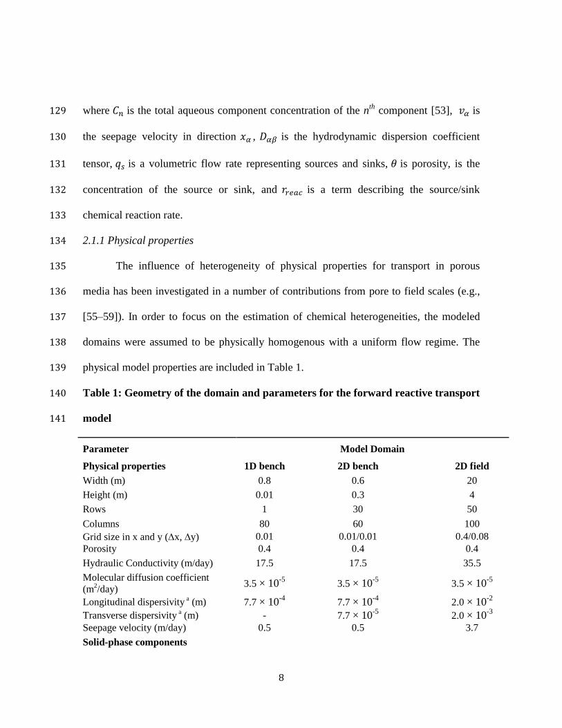
2.1.1 Physical properties 134

The influence of heterogeneity of physical properties for transport in porous 135

media has been investigated in a number of contributions from pore to field scales (e.g., 136

[55–59]). In order to focus on the estimation of chemical heterogeneities, the modeled 137

domains were assumed to be physically homogenous with a uniform flow regime. The 138

physical model properties are included in Table 1. 139

Table 1: Geometry of the domain and parameters for the forward reactive transport 140

model 141

Parameter Model Domain

Physical properties 1D bench 2D bench 2D field

Width (m) 0.8 0.6 20

Height (m) 0.01 0.3 4

Rows 1 30 50

Columns 80 60 100

Grid size in x and y (x, y) 0.01 0.01/0.01 0.4/0.08

Porosity 0.4 0.4 0.4

Hydraulic Conductivity (m/day) 17.5 17.5 35.5

Molecular diffusion coefficient

(m2/day)

3.5 × 10-5

3.5 × 10-5

3.5 × 10-5

Longitudinal dispersivity a (m) 7.7 × 10

-4 7.7 × 10

-4 2.0 × 10

-2

Transverse dispersivity a (m) - 7.7 × 10

-5 2.0 × 10

-3

Seepage velocity (m/day) 0.5 0.5 3.7

Solid-phase components

9

Concentration pyrite b (mg/kg soil) 7498.8 7498.8 2249.6

Concentration As (mg/kg soil) 70.3 70.3 21.1

As in pyrite (wt %) 0.94% 0.94% 0.94%

Influent aqueous concentrations (mol L-1

)

pH HCO3- Cl

- FeT Na

+ DO SO4

2- AsT

7 1.0 × 10-3

1.0 × 10-3

0 1.82 × 10-3

2.75 × 10-3

1.0 × 10-6

0 a values consistent with those reported in high-resolution laboratory [60] and field investigations [61,62] b values within range of concentrations listed in [63]

142

2.1.2 Chemical reaction framework 143

The forward simulations were based on a reaction network including 57 aqueous 144

equilibrium speciation half reactions, 2 kinetic mineral reactions, 13 surface 145

complexation reactions and reproduced scenarios in which an initially anoxic solution is 146

displaced by an aerated solution of the same ionic composition containing 2.75 × 10-4

147

mol/L of dissolved oxygen. We focus on the redox reaction resulting in the oxidative 148

dissolution of As-bearing pyrite due to the introduction of oxygenated water. The 149

chemical composition of the influent solution (Table 1) is identical to the initial solution 150

except the initial solution is anoxic and does not contain oxidized species. The reaction 151

network is similar to networks used in previous studies of arsenic reactive transport (e.g. 152

[64,65]) The introduction of oxygen into the previously anoxic domain results in the 153

kinetic oxidative dissolution of As-bearing pyrite. Briefly, the rate of pyrite oxidation was 154

defined by the following expression developed by [66] and previously used in field 155

applications [48,67]: 156

𝑟𝑝𝑦𝑟 = 𝐶𝑂2

0.5𝐶𝐻+−0.11 (10−10.19

𝐴𝑝𝑦𝑟

𝑉) (

𝐶

𝐶0)

𝑝𝑦𝑟

0.67

(2)

where rpyr is the rate of pyrite oxidation (mol/L/s), and CO2 and CH+ are the aqueous 157

concentrations of oxygen and hydrogen ions, respectively (mol/L). Apyr/V is the ratio of 158

10

pyrite surface area to the volume of solution and is set to 115 [48]. C/C0 is a factor 159

accounting for surface area changes resulting from the dissolution of pyrite. While 160

reaction (1) is slightly pH dependent, the bicarbonate in the groundwater buffers the 161

solution pH. The release of As(III) was simulated as stoichiometrically linked to the 162

oxidation of pyrite [50,64,65] which follows the following reaction: 163

𝐹𝑒𝑆2 + 3.75𝑂2 + 0.5𝐻2𝑂 → 𝐹𝑒3+ + 2𝑆𝑂42− + 𝐻+ (3)

The molar fraction of As to pyrite was set to 0.015 and was within previously reported 164

ranges of sedimentary materials [63,68]. 165

During the modeled dissolution of As-bearing pyrite, dissolved As(III) was 166

oxidized to As(V) which was the dominant As specie at steady-state. Additionally, 167

ferrous iron was released and subsequently oxidized to ferric iron. This resulted in the 168

precipitation of ferrihydrite (HFO) which can sorb As and retard the transport of this 169

contaminant. The rate of HFO formation is kinetic and was expressed as 170

𝑟𝐻𝐹𝑂 = 𝑘 (1 −

𝐼𝐴𝑃

𝐾𝑆𝑃) (3)

where rHFO is the rate of formation of HFO, k is an empirically derived constant set to 10-171

14 mol m

-2 s

-1 [65], and IAP/Ksp is the saturation ratio of ferrihydrite. The surface 172

complexation of As(III) and As(V) species on ferrihydrite was modeled as an 173

equilibrium-controlled process with a sorption site density of 0.2 mol/mol ferrihydrite 174

and a surface area of 600 m2/g [69]. 175

While other geochemical processes such as ligand exchange, competitive sorption 176

can affect arsenic transport (e.g., [16,70–72]), we focused on the oxidative dissolution of 177

reduced minerals as the main controlling mechanisms. We assumed DO concentrations 178

11

were controlled by the consumption of oxygen during the oxidation of sulfidic minerals. 179

Accordingly, we used distributed observations of DO to image the heterogeneous 180

distribution of As-bearing pyrite inclusions. In natural settings, DO consumption will be a 181

result of numerous geochemical processes inclusive of the oxidation of organic matter 182

and formation of oxide minerals such as manganese oxides which are both processes that 183

can affect the cycling of As in sediments (e.g., [18,73–75]). However, field-scale studies 184

have successfully simulated DO measurements by focusing on oxidative dissolution of 185

sulfidic minerals as the controlling process [64]. Therefore, we focus only on the 186

oxidative dissolution of As-bearing sulfides and precipitation of Fe (hydr)oxides as DO 187

consuming processes. Other processes can be accounted for with the error added to 188

simulated DO measurements as described below. 189

2.2 Inverse model 190

We used the PCGA to determine the spatial distribution of As-bearing pyrite from 191

a limited number of observations of DO concentrations while other parameters in 192

Equations (1) and (3) were assumed to be known and are provided in text. The PCGA is a 193

fast large-scale and joint inversion approach based on the geostatistical inverse method 194

[76,77], which is widely used for spatially distributed subsurface property calibration 195

problems. Here, we include a brief description of the geostatistical method followed by a 196

description of the PCGA. 197

2.2.1 Overview of the geostatistical approach 198

The objective of the geostatistical approach is to determine a vector of unknowns 199

from a vector of observations in a Bayesian framework. The observation equation is 200

given by: 201

12

𝒚 = ℎ(𝒔) + 𝒗 (4)

where y is the vector of observations, h is the forward model, s is the unknown variable, 202

and ν is a Gaussian term accounting for error in the observations and forward model. The 203

prior probability of s is assumed to be Gaussian with an unknown mean and a prior 204

covariance matrix Q. Using this assumption, the posterior pdf of s is calculated using 205

Bayes' theorem and the negative log likelihood of the posterior pdf forms the objective 206

function. By minimizing the objective function, the maximum a posteriori (MAP) 207

estimate or most likely value of s is obtained. This minimization of the objective function 208

is a nonlinear optimization problem that is commonly solved using iterative Gauss-209

Newton method where the initial guess is repeatedly updated to obtain a new As-bearing 210

pyrite distribution fitting the data. Specifically, in this application focused on imaging 211

reactive As-bearing minerals, y is the oxygen concentration at monitoring well, h is 212

reactive transport model, and s is spatially distributed As-bearing pyrite concentration. 213

While the geostatistical method is well suited for small- to moderate-scale inverse 214

problems, it becomes computationally challenging and costly for large-scale inversions. 215

Furthermore, the geostatistical method requires computation of the derivative of the 216

forward problem (Jacobian matrix, i.e., sensitivity of the observations to the unknowns) 217

which typically requires intrusive changes in the forward model code which is 218

challenging for multi-physics problems that utilize coupled forward models. 219

2.2.2 The principal component geostatistical approach 220

The PCGA expedites the geostatistical inversion by avoiding the direct evaluation 221

of the Jacobian. As a result, the number of numerical simulations can be reduced by a 222

factor of 10 or more with controlled accuracy in most cases. The PCGA avoids the direct 223

13

computation of the Jacobian by utilizing a low-rank approximation of the covariance Q 224

and a finite difference approximation of all matrix-vector products. Q is approximated 225

through: 226

𝐐 ≈ 𝐐𝑲 ≈ 𝒁𝒁𝑻 ≈ ∑ 𝜁𝑖𝜁𝑖𝑇

𝐾

𝑘=1

(5)

where 𝐐𝑲 is a rank-K approximation of Q, Z is a m by K matrix and 𝜁𝑖 is the i-th column 227

vector of Z. A fast method to obtain Equation (5) for large-scale covariance matrices is 228

explained in [3]. Approximately "K" forward simulation evaluations are needed to obtain 229

the inverse solution. By applying Equation (5), the PCGA can reduce the number of 230

numerical forward simulations greatly, usually up to a few hundred simulation runs, 231

which is highly beneficial for complex multi-species reactive transport problems, while 232

inverse solutions are almost the same as those obtained from the conventional 233

geostatistical approach as shown in [3]. 234

To enforce positivity in the estimation of As-bearing pyrite concentrations (Cpyr) 235

we used a square-root transformation: 236

𝐬 = √𝑪𝒑𝒚𝒓 (6)

This transformation can be seen as a simplified version of Box transformation [78], 237

which has been used to contaminant source identification applications (e.g., [79,80]). The 238

prior pdf of s was assumed to be Gaussian with unknown mean and exponential 239

covariance, Q. Numerical simulations and inversion were carried out on a Linux 240

workstation equipped with Intel 16 core 3.1 GHz processors and 128 GB RAM. 241

2.3 Problem setup 242

2.3.1 1-D bench 243

14

Beginning with a simplified domain, we simulated the oxidation of As-bearing 244

pyrite from a 1-D laboratory column of approximately 80 cm in length. The column 245

contained a 30 cm long inclusion of As-bearing pyrite in an otherwise homogenous 246

domain as shown in Figure 2b. The spatial and temporal changes in chemistry during the 247

forward reactive transport simulation are illustrated in Figure 2 for this 1-D domain. As a 248

result of oxidative dissolution, dissolved As, Fe(III) and SO42-

were released from the 249

pyritic mineral lens (Figure 2a). Ferric iron was released at a lower concentration than 250

SO42-

due to the precipitation of ferrihydrite (Figure 2b) and the lower abundance of Fe 251

than S in the pyritic minerals. The transport of As is also affected by the adsorption on 252

ferrihydrite surfaces. The 1-D column simulation reached pseudo-steady state conditions 253

after approximately 1.5-day simulation time (Figure 2c) in which the outlet 254

concentrations of dissolved chemical species were stable due to the slow dissolution of 255

As-bearing pyrite. After sufficient time, all the As-bearing pyrite will react and leave the 256

system, but due to the slow kinetics of As-bearing pyrite dissolution the system reaches a 257

pseudo-steady state in which the reaction byproduct concentrations are unchanged. 258

Among the dissolved chemical species, we assumed that the steady-state oxygen 259

concentrations were collected as the observation data for the inversion. This water 260

chemistry parameter was selected due to its key importance for oxidative dissolution of 261

reduced minerals and since currently available oxygen measurement sensors are 262

relatively inexpensive, accurate and operable in real-time. Such sensors have been 263

recently used to obtain high-resolution distributed measurements of oxygen in laboratory 264

setups [81–84] and field applications [85]. Gaussian random noise with a standard 265

deviation of 2% of the maximum oxygen consumption (10-6

mol/L) was added to the 266

15

observations to represent measurement and conceptual modeling errors in a well-267

controlled column experiment. The number of observations, unknowns and magnitude of 268

measurement error are listed in Table 2. 269

270

Table 2: Parameters of the inverse model carried out using the PCGA approach 271

Parameter Model Domain

1D bench 2D bench 2D field

Number of observations 5

20, 50, 75, 150

250

Number of unknowns 80

1800

5000

Number of principal components, K 80

32, 64, 96, 192

96

Covariance kernel, q exponential

exponential

exponential

Correlation length λ (m) 0.6

λx = 0.6, λz = 0.3

λx =20, λz = 4

Variance 0.1

0.1

0.1

Measurement error (mol/L) 10-6

10-6

2.5 × 10-5

, 5 × 10-5

272

16

273

Figure 2: (a) Spatial profiles of dissolved As, SO42-

and Fe(III) concentrations at 274

pseudo-steady state (2 days). (b) Solid-phase concentrations of pyrite at pseudo-275

steady state which diminished from initial concentration of 0.3 mol/L and Fe 276

(hydr)oxides which form as a result of pyrite oxidative dissolution and subsequent 277

oxidation of Fe(II). (c) Breakthrough curves of As and O2 concentrations (mol/L) at 278

the outlet of the domain. 279

280

17

2.3.2 2-D bench scale 281

Next, we imaged As-bearing pyrite inclusions in a 2-D bench-scale system. The 282

60 by 30 cm domain contained two 11 by 7 cm box-shaped inclusions in an otherwise 283

homogenous system as shown in Figure 4a. We assumed that five vertical arrays of 284

oxygen sensors were installed every 15 cm (x = 0, 0.15, 0.3, 0.45 and 0.6 m) (Figure 4a). 285

A measurement error of 4% of the maximum oxygen consumption was added to the 286

observed concentrations simulated from "true" As-bearing inclusions. Using this domain, 287

we examined (1) the number of forward simulation model runs, i.e., the number of 288

principal components (K) needed to obtain a reliable estimate of the unknown field and 289

(2) the effect of the number of measurements on the accuracy of the best estimate. 290

2.3.3 2-D field scale 291

To demonstrate the potential of the proposed approach to map complex patterns 292

of field-scale geochemical heterogeneities, we expanded our analysis to a 20 m × 4 m 293

cross-sectional domain. For this scenario, the spatial distribution pattern of geochemical 294

heterogeneity was generated stochastically: two realizations of Gaussian random fields 295

from an anisotropic exponential covariance model [86] were thresholded to obtain two 296

random binary As-bearing pyrite distributions as shown in Figure 7a. 297

3. Results and Discussion 298

3.1 1-D bench scale 299

The "true" field shown in Figure 3a was used to generate five steady-state 300

synthetic concentration measurements with observation locations displayed as red circles 301

in Figure 3c. Because this 1-D forward problem can be solved efficiently in 5 seconds, 302

the PCGA with all K = 80 principal components (i.e., equal to the number of grid cells) 303

18

was used to estimate the underlying As-bearing pyrite concentrations to illustrate how the 304

inversion approach performs for geochemical heterogeneity identification. In this case, 305

low-rank approximation was not used and the approximation error only comes from the 306

finite difference approximation in the inverse method. Inversion with smaller number of 307

principal components is presented in the 2-D simulations. While the initial guess was set 308

to a homogeneous As-bearing pyrite distribution with a concentration of 5000 mg/kg 309

across the entire domain, several initial guesses were tested and the inversion converged 310

to the same estimate for any reasonable choice of an initial guess. 311

312

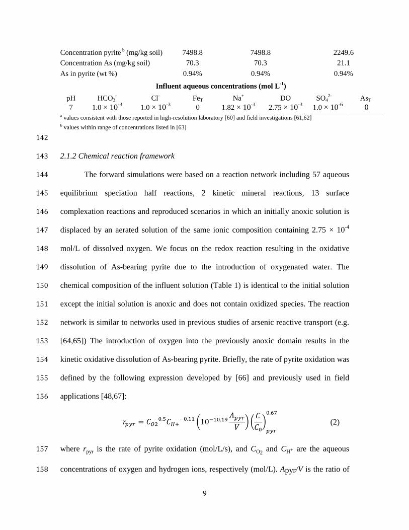
Figure 3: (a) True concentration (mg/kg) of As-bearing pyrite, (b) estimated 313

concentration (mg/kg), (c) steady-state oxygen concentration resulting from the 314

19

oxidative dissolution of true As-bearing pyrite and selected measurements (red 315

circles) with noise for the inversion and (d) simulated steady-state oxygen 316

concentrations resulting from the estimated As-bearing pyrite and reproduced 317

oxygen concentrations (red circles) at the monitoring locations 318

319

A total of 329 forward model runs (converged with 4 iterations) were used to 320

obtain the result on 16 processors in 5 minutes. Structural parameters such as noise level, 321

prior variance and correlation length were chosen using Q2/Cr criteria [87] which 322

provides a framework for selecting the model parameters to be used for the inversion. 323

The resulting parameter values are reported in Table 2. The inversion successfully 324

captures the location and magnitude of the true As-bearing pyrite concentration (Figure 325

3b) while the estimated distribution is smooth due to the Gaussian distribution 326

assumption of the prior. The true As-bearing pyrite distribution is located within the 95% 327

confidence interval (Figure 3b) of the inversion. Confidence interval was relatively wide 328

at the constant concentration boundary condition (x = 0 cm) and the most downstream (x 329

= 80 cm). Because of the fixed boundary condition at x = 0 cm and advective information 330

propagation, the information of measurements at both locations is almost zero, resulting 331

in the high uncertainty around the both ends. The estimated pyrite reproduces the DO 332

measurements accurately within measurement error as shown in Figure 3d. This simple 333

experiment demonstrates that a reasonable estimate can be achieved with a few hundred 334

simulation runs even with only a few sparse oxygen measurements. 335

3.2 2-D bench scale 336

20

The true field for a 2-D bench-scale domain (Figure 4a) was used to generate the 337

DO observation measurements in Figure 4a. These measurements were successively used 338

for the PCGA-based inversion to image the location and the concentration of the As-339

bearing reactive mineral inclusions in the 2-D domain. 340

341

Figure 4: The effect of the number of principal components (K) on the pyrite 342

distribution estimate. (a) shows the true pyrite distribution (first column) and 343

21

corresponding oxygen concentration (second column) along with the DO 344

measurements which are highlighted with black markers. The best estimates of 345

pyrite distribution, corresponding simulated oxygen concentration and variance of 346

estimate are shown for K = (b) 512, (c) 96, (d) 64, and (e) 32. 347

348

3.2.1 Effect of number of principal components (K) 349

Initially, it was assumed that each sensor array collected a DO depth profile with 350

measurements every 1 cm in depth, which amounts to a total of 150 measurements used 351

in the inversion. To investigate an optimal number of principal components in this 352

application, K = 512, 96, 64 and 32 principal components were used to estimate the 353

underlying pyrite concentration. Sixteen multiples of K values were assigned to take 354

advantage of parallel executions on the 16-core workstation. For K = 512, a total of 2576 355

forward simulations were executed to find a best estimate in around 10 hours; while for K 356

= 32, total 176 simulations were run in 40 minutes. 357

The best estimates are presented in Figure 4b-4e. Even with only 32 principal 358

components, the inversion was able to capture the location and magnitude of the 359

underlying pyrite lenses. Also the best estimate of the oxygen consumption, obtained 360

with the different numbers of principal components, closely reproduced the pattern 361

observed in the true field. We used the root mean square error (RMSE) as a quantitative 362

metric to assess the performance of the inversion. Calculating the RMSE of the best 363

estimate as compared to the true distribution, we observed that it does not change 364

significantly as a function of K (Figure 6a). This is due to the simple geometry of the true 365

22

concentration field, which only requires a relatively small number of simulations to 366

obtain a reasonable estimate. 367

While the estimated location of the pyrite lenses can be accurately determined 368

with a small number of principal components, the estimation uncertainty was generally 369

underestimated because of the approximation used in Equation (4). Increasing K resulted 370

in decreased RMSE of the uncertainty as shown in Figure 6c. Thus, it is recommended 371

that more principal components be added to accurately quantify estimation uncertainty. 372

While this requires more simulation runs, starting with a moderate number of K values 373

and increase K when convergence is achieved, the correct estimation uncertainty can be 374

gained. 375

3.2.2 Effect of number of measurement points 376

To evaluate the efficiency of the inversion approach, the effect of the number of 377

data measurements used in the inversion was examined. Figures 5b-5e show the best 378

estimates for the location and concentration of the As-bearing pyrite inclusions, the 379

corresponding oxygen consumption and the computed estimation uncertainty with 150, 380

75, 50, 20 measurements which corresponds to 1, 2, 3 and 7.5 cm vertical spacing of 381

measurement locations, respectively. Good estimates of As-bearing pyrite distribution 382

were obtained for the cases considering at least 50 data points. The quality of the image 383

deteriorates significantly for the case using only 20 measurement points. Inversion with 384

20 measurements (7.5-cm spacing which is larger than the 7-cm height of the pyrite lens) 385

resulted in poor identification of the pyrite distribution. In this case, the method did not 386

capture the bottom-right inclusion and also the concentration range of the image becomes 387

rather dissimilar from the true field. This results from the impossibility of the very sparse 388

23

observation network to capture the oxygen concentration gradients due to oxidative 389

dissolution in the lower part of the domain. Again, we used RMSE to quantitatively 390

evaluate the performance of the inversion as a function of the number of observation 391

points. We observed that the RMSE decreases significantly with increasing number of 392

observations (Figure 6b). However, it should be noted that such RMSE decrease tends to 393

be less pronounced with larger number of measurements for the distribution of 394

measurements examined in this domain. The results emphasize that even with a relatively 395

small number of observations (~50 measurement points), the proposed approach was able 396

to identify the location and magnitude of the As-bearing pyrite distribution while smaller 397

number of data measurements could result in errors in the estimation of the sulfidic 398

mineral location. 399

24

400

Figure 5: Effect of the number of measurements on pyrite estimates. The true pyrite 401

and oxygen distributions are shown in (a). The best estimates of pyrite distribution, 402

corresponding simulated oxygen concentration and uncertainty are shown for (b) 403

150, (c) 75, (d) 50, and (e) 20 total measurements. Black circles highlight the location 404

of the dissolved oxygen measurements. 405

25

406

407

Figure 6: RMSE as a function of (a) the number of principal components, (b) 408

number of measurement points used in the inversion and (c) RMSE relative to 409

uncertainty of the best estimate for 512 principal components. 410

3.3 2-D field scale 411

Lastly, field-scale characterizations were performed to study potential 412

applications of the inversion method. Two random heterogeneous fields were generated 413

and tested as shown in Figures 7a and 7b. Oxygen sensor arrays are assumed to be 414

located at x = 0, 4, 8, 12, 16 and 20 m and at each array, sensors were installed every 0.25 415

m corresponding to a total of 96 measurement points for this analysis. Larger error of 10% 416

and 20% of the maximum oxygen consumption was added to the simulated 417

concentrations to reflect higher uncertainty at the field-scale. The best estimates are 418

shown in Figure 7. With measurement error of 10% and irregularly distributed 419

heterogeneities, the inversion method can accurately identify the location of the As-420

bearing pyrite lenses. At 20% measurement error, difficulties were encountered in 421

capturing the location and magnitude of all the heterogeneities, particularly small pyrite 422

26

lenses. We also performed forward simulations using the best estimate of the spatial 423

distribution of pyrite to analyze the capability of the inversion results to reproduce the 424

arsenic plumes from the true pyrite distribution. The estimated As-bearing pyrite 425

locations and magnitude reproduced the main features and the multiple plumes of 426

dissolved As within the simulated aquifer (Figure 8). With 10% measurement error, the 427

location of all high As concentration plumes were accurately captured although the 428

magnitude was slightly underestimated. With 20% measurement error the main arsenic 429

plumes are still correctly located but not all chemical heterogeneities causing As release 430

were captured; thus, not all As plumes were reproduced and the magnitude of As 431

concentration was underestimated, in particular in the upper plumes. 432

433

27

Figure 7: Best estimate maps for randomly distributed heterogeneous fields of As-434

bearing pyrite for (a) Case 1 with (c) 10% error, (e) 20% error, and for (b) Case 2 435

with (d) 10% error and (f) 20% error. 436

437

Figure 8: Dissolved arsenic concentrations at pseudo steady state for (a) the true 438

As-bearing pyrite distribution and (b) the estimated pyrite distribution obtained in 439

Figure 7c with 10% measurement error and (c) the estimated pyrite distribution 440

obtained in Figure 7e with 20% measurement error. 441

442

Field-scale imaging of chemically reactive heterogeneities can be useful for a 443

variety of applications. For example, one potential application includes managed aquifer 444

28

recharge (MAR) projects where shifts in native aquifer chemistry can mobilize 445

contaminants including As [48,50,63,88,89]. MAR sites in which common water quality 446

parameters are regularly monitored are potentially well-suited sites for inverse reactive 447

transport modeling methods to image reactive geochemical heterogeneities due to 448

installation of water quality monitoring well networks. Additionally, MAR sites that 449

employ aquifer storage and recovery (ASR) wells provide a unique reversal in flow 450

regime which can further enhance inversion results. Generally, upstream locations have 451

more information available through the downstream measurements. Thus, we tested a 452

scenario with reversed flow conditions, by switching downstream and upstream locations. 453

This improves the imaging results of previously down-gradient heterogeneities that 454

contained higher uncertainty. Specifically, Figure 9 shows a simulated inversion for the 455

heterogeneous field-case in which reverse flow data were used to image pyrite lenses 456

(Figure 9b) and the forward and reverse flow measurements were used in conjunction 457

(Figure 9c) to further enhance the imaging of the reactive mineral inclusions. 458

Furthermore, in the reverse flow case, previously unidentified pyrite lenses (Figure 7f) 459

are now characterized relatively well, and the combination of two different data sets with 460

higher measurement error provides a comparable result to Figure 7d, which uses 461

unidirectional flow but with smaller measurement error. RMSEs for forward flow (Figure 462

7f), reverse flow (Figure 9b) and joint (Figure 9c) cases with respect to the true field 463

(Figure 7b) are computed as 623, 585 and 557 mg/kg respectively, while RMSE of the 464

case with unidirectional forward flow and 10% measurement error (Figure 7d) is 514 465

mg/kg. 466

29

467

Figure 9: (a) Random, true As-bearing pyrite distribution, (b) the best estimate 468

using only information for a reversed flow regime with 10% noise (flow right-to-469

left), and (c) the best estimate using data measurements from both left-to-right flow 470

regime (Figure 7f) and the right-to-left flow regime. 471

4. Conclusion 472

Our results show that the proposed PCGA-based inverse reactive transport 473

modeling approach can be used to image irregularly distributed As-bearing pyrite 474

inclusions at various scales and has the potential to map complex distributions of reactive 475

30

subsurface properties based on the measurement of reactive dissolved constituents 476

commonly measured in groundwater. While we develop this method using a simplified 477

modeling approach, the method can be adapted to accommodate more complex reaction 478

networks. This application and similar approaches will be facilitated by rapid advances in 479

computational methods and sensor technology. 480

We demonstrated the capability and potential of inverse methods for geochemical 481

tomography by focusing on As-bearing minerals, and there are numerous additional 482

applications in which these methods can greatly help characterize subsurface 483

geochemical heterogeneities. Possible directions for exploring include: testing the 484

proposed approach with experimental observations, considering the value of information 485

of transient observations taken in different sampling events, using observations of 486

multiple parameters (e.g., dissolved oxygen with pH or other dissolved species) perturbed 487

by specific geochemical reactions. 488

Of key importance is the deployment of these methods for the simultaneous 489

characterization of both physical and chemical subsurface properties. In this study, we 490

focused on characterizing reactive chemical properties as a proof-of-concept; however, 491

coupling of physical and chemical subsurface imaging is essential for ensuring proper 492

management of groundwater aquifers and enhancing the reliability of process-based 493

reactive transport models. Additionally, the accurate determination of spatially 494

distributed physical and geochemical properties in field systems provides valuable 495

understanding of the influence of aquifer characteristics on contaminant behavior. 496

497

498

31

499

Acknowledgements 500

The research was funded by the National Science Foundation through its ReNUWIt 501

Engineering Research Center (www.renuwit.org; NSF EEC-1028968) and a National 502

Science Foundation Graduate Research Fellowship (NSF GRFP). M.R. acknowledges the 503

support of the Baden-Württemberg Stiftung under the Eliteprogram for postdocs. 504

505

References 506

[1] Cardiff M, Barrash W, Kitanidis PK. A field proof-of-concept of aquifer imaging using 3-507 D transient hydraulic tomography with modular, temporarily-emplaced equipment. 508 Water Resour Res 2012;48:W05531. doi:10.1029/2011WR011704. 509

[2] Cardiff M, Barrash W, Kitanidis P k., Malama B, Revil A, Straface S, et al. A Potential-510 Based Inversion of Unconfined Steady-State Hydraulic Tomography. Ground Water 511 2009;47:259–70. doi:10.1111/j.1745-6584.2008.00541.x. 512

[3] Lee J, Kitanidis PK. Large-scale hydraulic tomography and joint inversion of head and 513 tracer data using the Principal Component Geostatistical Approach (PCGA). Water 514 Resour Res 2014;50:5410–27. doi:10.1002/2014WR015483. 515

[4] Zhu J, Yeh T-CJ. Characterization of aquifer heterogeneity using transient hydraulic 516 tomography. Water Resour Res 2005;41:W07028. doi:10.1029/2004WR003790. 517

[5] Revil A, Karaoulis M, Johnson T, Kemna A. Review: Some low-frequency electrical 518 methods for subsurface characterization and monitoring in hydrogeology. Hydrogeol J 519 2012;20:617–58. doi:10.1007/s10040-011-0819-x. 520

[6] Slater L. Near Surface Electrical Characterization of Hydraulic Conductivity: From 521 Petrophysical Properties to Aquifer Geometries—A Review. Surv Geophys 522 2007;28:169–97. doi:10.1007/s10712-007-9022-y. 523

[7] Davis JL, Annan AP. Ground-penetrating radar for high-resolution mapping of soil and 524 rock stratigraphy. Geophys Prospect 1989;37:531–51. 525

[8] Kowalsky MB, Finsterle S, Rubin Y. Estimating flow parameter distributions using 526 ground-penetrating radar and hydrological measurements during transient flow in the 527 vadose zone. Adv Water Resour 2004;27:583–99. 528 doi:10.1016/j.advwatres.2004.03.003. 529

[9] Allen-King RM, Kalinovich I, Dominic DF, Wang G, Polmanteer R, Divine D. 530 Hydrophobic organic contaminant transport property heterogeneity in the Borden 531 Aquifer. Water Resour Res 2015;51:1723–43. doi:10.1002/2014WR016161. 532

[10] Allen-King RM, Divine DP, Robin MJL, Alldredge JR, Gaylord DR. Spatial distributions of 533 perchloroethylene reactive transport parameters in the Borden Aquifer. Water Resour 534 Res 2006;42:W01413. doi:10.1029/2005WR003977. 535

[11] Barber II LB, Thurman EM, Runnells DD. Geochemical heterogeneity in a sand and 536 gravel aquifer: Effect of sediment mineralogy and particle size on the sorption of 537

32

chlorobenzenes. J Contam Hydrol 1992;9:35–54. doi:10.1016/0169-7722(92)90049-538 K. 539

[12] Ritzi RW, Huang L, Ramanathan R, Allen-King RM. Horizontal spatial correlation of 540 hydraulic and reactive transport parameters as related to hierarchical sedimentary 541 architecture at the Borden research site. Water Resour Res 2013;49:1901–13. 542 doi:10.1002/wrcr.20165. 543

[13] Redman AD, Macalady DL, Ahmann D. Natural Organic Matter Affects Arsenic 544 Speciation and Sorption onto Hematite. Environ Sci Technol 2002;36:2889–96. 545 doi:10.1021/es0112801. 546

[14] Weng L, Van Riemsdijk WH, Hiemstra T. Effects of Fulvic and Humic Acids on Arsenate 547 Adsorption to Goethite: Experiments and Modeling. Environ Sci Technol 548 2009;43:7198–204. doi:10.1021/es9000196. 549

[15] Wang S, Mulligan CN. Effect of natural organic matter on arsenic release from soils and 550 sediments into groundwater. Environ Geochem Health 2006;28:197–214. 551 doi:10.1007/s10653-005-9032-y. 552

[16] Sharma P, Rolle M, Kocar B, Fendorf S, Kappler A. Influence of Natural Organic Matter 553 on As Transport and Retention. Environ Sci Technol 2011;45:546–53. 554 doi:10.1021/es1026008. 555

[17] Stuckey JW, Schaefer MV, Kocar BD, Dittmar J, Pacheco JL, Benner SG, et al. Peat 556 formation concentrates arsenic within sediment deposits of the Mekong Delta. 557 Geochim Cosmochim Acta 2015;149:190–205. doi:10.1016/j.gca.2014.10.021. 558

[18] McArthur JM, Banerjee DM, Hudson-Edwards KA, Mishra R, Purohit R, Ravenscroft P, 559 et al. Natural organic matter in sedimentary basins and its relation to arsenic in anoxic 560 ground water: the example of West Bengal and its worldwide implications. Appl 561 Geochem 2004;19:1255–93. doi:10.1016/j.apgeochem.2004.02.001. 562

[19] Molinari A, Guadagnini L, Marcaccio M, Straface S, Sanchez-Vila X, Guadagnini A. 563 Arsenic release from deep natural solid matrices under experimentally controlled 564 redox conditions. Sci Total Environ 2013;444:231–40. 565 doi:10.1016/j.scitotenv.2012.11.093. 566

[20] Englert A, Hubbard SS, Williams KH, Li L, Steefel CI. Feedbacks Between Hydrological 567 Heterogeneity and Bioremediation Induced Biogeochemical Transformations. Environ 568 Sci Technol 2009;43:5197–204. doi:10.1021/es803367n. 569

[21] Li L, Gawande N, Kowalsky MB, Steefel CI, Hubbard SS. Physicochemical Heterogeneity 570 Controls on Uranium Bioreduction Rates at the Field Scale. Environ Sci Technol 571 2011;45:9959–66. doi:10.1021/es201111y. 572

[22] Steefel CI, DePaolo DJ, Lichtner PC. Reactive transport modeling: An essential tool and 573 a new research approach for the Earth sciences. Earth Planet Sci Lett 2005;240:539–574 58. doi:10.1016/j.epsl.2005.09.017. 575

[23] Li L, Salehikhoo F, Brantley SL, Heidari P. Spatial zonation limits magnesite dissolution 576 in porous media. Geochim Cosmochim Acta 2014;126:555–73. 577 doi:10.1016/j.gca.2013.10.051. 578

[24] Li L, Steefel CI, Kowalsky MB, Englert A, Hubbard SS. Effects of physical and 579 geochemical heterogeneities on mineral transformation and biomass accumulation 580 during biostimulation experiments at Rifle, Colorado. J Contam Hydrol 2010;112:45–581 63. doi:10.1016/j.jconhyd.2009.10.006. 582

[25] Chen J, Hubbard SS, Williams KH. Data-driven approach to identify field-scale 583 biogeochemical transitions using geochemical and geophysical data and hidden 584 Markov models: Development and application at a uranium-contaminated aquifer. 585 Water Resour Res 2013;49:6412–24. doi:10.1002/wrcr.20524. 586

33

[26] Chen J, Hubbard SS, Williams KH, Flores Orozco A, Kemna A. Estimating the 587 spatiotemporal distribution of geochemical parameters associated with biostimulation 588 using spectral induced polarization data and hierarchical Bayesian models: 589 ESTIMATING GEOCHEMICAL PARAMETERS USING SIP DATA. Water Resour Res 590 2012;48:n/a – n/a. doi:10.1029/2011WR010992. 591

[27] Flores Orozco A, Williams KH, Long PE, Hubbard SS, Kemna A. Using complex 592 resistivity imaging to infer biogeochemical processes associated with bioremediation 593 of an uranium-contaminated aquifer. J Geophys Res Biogeosciences 2011;116:G03001. 594 doi:10.1029/2010JG001591. 595

[28] Hubbard SS, Williams K, Conrad ME, Faybishenko B, Peterson J, Chen J, et al. 596 Geophysical Monitoring of Hydrological and Biogeochemical Transformations 597 Associated with Cr(VI) Bioremediation. Environ Sci Technol 2008;42:3757–65. 598 doi:10.1021/es071702s. 599

[29] Scheibe TD, Fang Y, Murray CJ, Roden EE, Chen J, Chien Y-J, et al. Transport and 600 biogeochemical reaction of metals in a physically and chemically heterogeneous 601 aquifer. Geosphere 2006;2:220–35. doi:10.1130/GES00029.1. 602

[30] Williams KH, Kemna A, Wilkins MJ, Druhan J, Arntzen E, N’Guessan AL, et al. 603 Geophysical Monitoring of Coupled Microbial and Geochemical Processes During 604 Stimulated Subsurface Bioremediation. Environ Sci Technol 2009;43:6717–23. 605 doi:10.1021/es900855j. 606

[31] Williams KH, Ntarlagiannis D, Slater LD, Dohnalkova A, Hubbard SS, Banfield JF. 607 Geophysical Imaging of Stimulated Microbial Biomineralization. Environ Sci Technol 608 2005;39:7592–600. doi:10.1021/es0504035. 609

[32] Sassen DS, Hubbard SS, Bea SA, Chen J, Spycher N, Denham ME. Reactive facies: An 610 approach for parameterizing field-scale reactive transport models using geophysical 611 methods. Water Resour Res 2012;48:W10526. doi:10.1029/2011WR011047. 612

[33] Wainwright HM, Chen J, Sassen DS, Hubbard SS. Bayesian hierarchical approach and 613 geophysical data sets for estimation of reactive facies over plume scales. Water Resour 614 Res 2014;50:4564–84. doi:10.1002/2013WR013842. 615

[34] Cardiff M, Kitanidis PK. Fitting Data Under Omnidirectional Noise: A Probabilistic 616 Method for Inferring Petrophysical and Hydrologic Relations. Math Geosci 617 2010;42:877–909. doi:10.1007/s11004-010-9301-x. 618

[35] Smith E, Naidu R, Alston AM. Arsenic in the Soil Environment: A Review. In: Sparks DL, 619 editor. Adv. Agron., vol. 64, Academic Press; 1998, p. 149–95. 620

[36] Smedley PL, Kinniburgh DG. A review of the source, behaviour and distribution of 621 arsenic in natural waters. Appl Geochem 2002;17:517–68. doi:10.1016/S0883-622 2927(02)00018-5. 623

[37] Fendorf S, Nico PS, Kocar BD, Masue Y, Tufano KJ. Chapter 12 - Arsenic Chemistry in 624 Soils and Sediments. In: Gräfe BS and M, editor. Dev. Soil Sci., vol. 34, Elsevier; 2010, p. 625 357–78. 626

[38] Borch T, Kretzschmar R, Kappler A, Cappellen PV, Ginder-Vogel M, Voegelin A, et al. 627 Biogeochemical Redox Processes and their Impact on Contaminant Dynamics. Environ 628 Sci Technol 2010;44:15–23. doi:10.1021/es9026248. 629

[39] Haberer CM, Rolle M, Cirpka OA, Grathwohl P. Oxygen Transfer in a Fluctuating 630 Capillary Fringe. Vadose Zone J 2012;11:vzj2011.0056. doi:10.2136/vzj2011.0056. 631

[40] Kocar BD, Polizzotto ML, Benner SG, Ying SC, Ung M, Ouch K, et al. Integrated 632 biogeochemical and hydrologic processes driving arsenic release from shallow 633 sediments to groundwaters of the Mekong delta. Appl Geochem 2008;23:3059–71. 634 doi:10.1016/j.apgeochem.2008.06.026. 635

34

[41] Farnsworth CE, Hering JG. Inorganic geochemistry and redox dynamics in bank 636 filtration settings. Environ Sci Technol 2011;45:5079–87. doi:10.1021/es2001612. 637

[42] Polizzotto ML, Kocar BD, Benner SG, Sampson M, Fendorf S. Near-surface wetland 638 sediments as a source of arsenic release to ground water in Asia. Nature 639 2008;454:505–8. doi:10.1038/nature07093. 640

[43] Stuckey JW, Schaefer MV, Benner SG, Fendorf S. Reactivity and speciation of mineral-641 associated arsenic in seasonal and permanent wetlands of the Mekong Delta. Geochim 642 Cosmochim Acta 2015;171:143–55. doi:10.1016/j.gca.2015.09.002. 643

[44] Postma D, Larsen F, Minh Hue NT, Duc MT, Viet PH, Nhan PQ, et al. Arsenic in 644 groundwater of the Red River floodplain, Vietnam: Controlling geochemical processes 645 and reactive transport modeling. Geochim Cosmochim Acta 2007;71:5054–71. 646 doi:10.1016/j.gca.2007.08.020. 647

[45] Frohne T, Rinklebe J, Diaz-Bone RA, Du Laing G. Controlled variation of redox 648 conditions in a floodplain soil: Impact on metal mobilization and biomethylation of 649 arsenic and antimony. Geoderma 2011;160:414–24. 650 doi:10.1016/j.geoderma.2010.10.012. 651

[46] Molinari A, Ayora C, Marcaccio M, Guadagnini L, Sanchez-Vila X, Guadagnini A. 652 Geochemical modeling of arsenic release from a deep natural solid matrix under 653 alternated redox conditions. Environ Sci Pollut Res 2013;21:1628–37. 654 doi:10.1007/s11356-013-2054-6. 655

[47] Mirecki JE, Bennett MW, López-Baláez MC. Arsenic control during aquifer storage 656 recovery cycle tests in the Floridan Aquifer. Ground Water 2013;51:539–49. 657 doi:10.1111/j.1745-6584.2012.01001.x. 658

[48] Prommer H, Stuyfzand PJ. Identification of Temperature-Dependent Water Quality 659 Changes during a Deep Well Injection Experiment in a Pyritic Aquifer. Environ Sci 660 Technol 2005;39:2200–9. doi:10.1021/es0486768. 661

[49] Vanderzalm JL, Dillon PJ, Barry KE, Miotlinski K, Kirby JK, Le Gal La Salle C. Arsenic 662 mobility and impact on recovered water quality during aquifer storage and recovery 663 using reclaimed water in a carbonate aquifer. Appl Geochem 2011;26:1946–55. 664 doi:10.1016/j.apgeochem.2011.06.025. 665

[50] Wallis I, Prommer H, Simmons CT, Post V, Stuyfzand PJ. Evaluation of Conceptual and 666 Numerical Models for Arsenic Mobilization and Attenuation during Managed Aquifer 667 Recharge. Environ Sci Technol 2010;44:5035–41. doi:10.1021/es100463q. 668

[51] Kitanidis PK, Lee J. Principal Component Geostatistical Approach for large-dimensional 669 inverse problems. Water Resour Res 2014;50:5428–43. doi:10.1002/2013WR014630. 670

[52] Harbaugh AW, Banta ER, Hill MC, McDonald MG. MODFLOW-2000, The U.S. Geological 671 Survey Modular Ground-Water Model - User Guide to Modularization Concepts and the 672 Ground-Water Flow Process. United States Geological Survey; 2000. 673

[53] Prommer H, Barry DA, Zheng C. MODFLOW/MT3DMS-based reactive multicomponent 674 transport modeling. Ground Water 2003;41:247–57. 675

[54] Parkhurst D, Appelo C. User’s guide to PHREEQC - A computer program for speciation, 676 reaction-path, ID-transport, and inverse geochemical calculations. U.S. Geological 677 Survey Water Resources Investigations Report; 1999. 678

[55] Fiori A, Jankovic I, Dagan G. The impact of local diffusion upon mass arrival of a passive 679 solute in transport through three-dimensional highly heterogeneous aquifers. Adv 680 Water Resour 2011;34:1563–73. doi:10.1016/j.advwatres.2011.08.010. 681

[56] Kitanidis PK. The concept of the Dilution Index. Water Resour Res 1994;30:2011–26. 682 doi:10.1029/94WR00762. 683

[57] Hochstetler DL, Rolle M, Chiogna G, Haberer CM, Grathwohl P, Kitanidis PK. Effects of 684 compound-specific transverse mixing on steady-state reactive plumes: Insights from 685

35

pore-scale simulations and Darcy-scale experiments. Adv Water Resour 2013;54:1–10. 686 doi:10.1016/j.advwatres.2012.12.007. 687

[58] Rolle M, Chiogna G, Hochstetler DL, Kitanidis PK. On the importance of diffusion and 688 compound-specific mixing for groundwater transport: An investigation from pore to 689 field scale. J Contam Hydrol 2013;153:51–68. doi:10.1016/j.jconhyd.2013.07.006. 690

[59] Rolle M, Kitanidis PK. Effects of compound-specific dilution on transient transport and 691 solute breakthrough: A pore-scale analysis. Adv Water Resour 2014;71:186–99. 692 doi:10.1016/j.advwatres.2014.06.012. 693

[60] Rolle M, Eberhardt C, Chiogna G, Cirpka OA, Grathwohl P. Enhancement of dilution and 694 transverse reactive mixing in porous media: Experiments and model-based 695 interpretation. J Contam Hydrol 2009;110:130–42. 696 doi:10.1016/j.jconhyd.2009.10.003. 697

[61] Prommer H, Tuxen N, Bjerg PL. Fringe-Controlled Natural Attenuation of Phenoxy 698 Acids in a Landfill Plume:  Integration of Field-Scale Processes by Reactive Transport 699 Modeling. Environ Sci Technol 2006;40:4732–8. doi:10.1021/es0603002. 700

[62] Prommer H, Anneser B, Rolle M, Einsiedl F, Griebler C. Biogeochemical and Isotopic 701 Gradients in a BTEX/PAH Contaminant Plume: Model-Based Interpretation of a High-702 Resolution Field Data Set. Environ Sci Technol 2009;43:8206–12. 703 doi:10.1021/es901142a. 704

[63] Price RE, Pichler T. Abundance and mineralogical association of arsenic in the 705 Suwannee Limestone (Florida): Implications for arsenic release during water–rock 706 interaction. Chem Geol 2006;228:44–56. doi:10.1016/j.chemgeo.2005.11.018. 707

[64] Wallis I, Prommer H, Pichler T, Post V, B. Norton S, Annable MD, et al. Process-Based 708 Reactive Transport Model To Quantify Arsenic Mobility during Aquifer Storage and 709 Recovery of Potable Water. Environ Sci Technol 2011;45:6924–31. 710 doi:10.1021/es201286c. 711

[65] Descourvieres C, Prommer H, Oldham C, Greskowiak J, Hartog N. Kinetic Reaction 712 Modeling Framework for Identifying and Quantifying Reductant Reactivity in 713 Heterogeneous Aquifer Sediments. Environ Sci Technol 2010;44:6698–705. 714 doi:10.1021/es101661u. 715

[66] Williamson MA, Rimstidt JD. The kinetics and electrochemical rate-determining step of 716 aqueous pyrite oxidation. Geochim Cosmochim Acta 1994;58:5443–54. 717 doi:10.1016/0016-7037(94)90241-0. 718

[67] Eckert P, Appelo C a. J. Hydrogeochemical modeling of enhanced benzene, toluene, 719 ethylbenzene, xylene (BTEX) remediation with nitrate. Water Resour Res 2002;38:5–720 1. doi:10.1029/2001WR000692. 721

[68] Kolker A, Haack SK, Cannon WF, Westjohn DB, Kim M-J, Nriagu J, et al. Arsenic in 722 southeastern Michigan. In: Welch AH, Stollenwerk KG, editors. Arsen. Ground Water, 723 Springer US; 2003, p. 281–94. 724

[69] Dzombak DA, Morel FMM. Surface complexation modeling: Hydrous ferric oxide. 725 Wiley, New York; 1990. 726

[70] Fendorf S, Herbel M, Tufano K, Kocar BD. Biogeochemical Processes Controlling the 727 Cycling of Arsenic in Soils and Sediments. Biophys.-Chem. Process. Heavy Met. Met. 728 Soil Environ., John Wiley & Sons; 2007. 729

[71] Dixit S, Hering JG. Comparison of arsenic(V) and arsenic(III) sorption onto iron oxide 730 minerals: implications for arsenic mobility. Environ Sci Technol 2003;37:4182–9. 731

[72] Appelo CAJ, Van Der Weiden MJJ, Tournassat C, Charlet L. Surface Complexation of 732 Ferrous Iron and Carbonate on Ferrihydrite and the Mobilization of Arsenic. Environ 733 Sci Technol 2002;36:3096–103. doi:10.1021/es010130n. 734

36

[73] Manning BA, Fendorf SE, Bostick B, Suarez DL. Arsenic(III) Oxidation and Arsenic(V) 735 Adsorption Reactions on Synthetic Birnessite. Environ Sci Technol 2002;36:976–81. 736 doi:10.1021/es0110170. 737

[74] Scott MJ, Morgan JJ. Reactions at Oxide Surfaces. 1. Oxidation of As(III) by Synthetic 738 Birnessite. Environ Sci Technol 1995;29:1898–905. doi:10.1021/es00008a006. 739

[75] Ying SC, Kocar BD, Griffis SD, Fendorf S. Competitive Microbially and Mn Oxide 740 Mediated Redox Processes Controlling Arsenic Speciation and Partitioning. Environ Sci 741 Technol 2011;45:5572–9. doi:10.1021/es200351m. 742

[76] Kitanidis PK. Quasi-Linear Geostatistical Theory for Inversing. Water Resour Res 743 1995;31:2411–9. doi:10.1029/95WR01945. 744

[77] Kitanidis PK. On the geostatistical approach to the inverse problem. Adv Water Resour 745 1996;19:333–42. doi:10.1016/0309-1708(96)00005-X. 746

[78] Box GEP, Cox DR. An Analysis of Transformations. J R Stat Soc Ser B Methodol 747 1964;26:211–52. 748

[79] Snodgrass MF, Kitanidis PK. A geostatistical approach to contaminant source 749 identification. Water Resour Res 1997;33:537–46. doi:10.1029/96WR03753. 750

[80] Kitanidis PK, Shen K-F. Geostatistical interpolation of chemical concentration. Adv 751 Water Resour 1996;19:369–78. doi:10.1016/0309-1708(96)00016-4. 752

[81] Haberer CM, Rolle M, Cirpka OA, Grathwohl P. Oxygen transfer in a fluctuating 753 capillary fringe. Vadose Zone J 2012; doi:10.2136/vzj2011.0056. 754

[82] Haberer CM, Muniruzzaman M, Grathwohl P, Rolle M. Diffusive–Dispersive and 755 Reactive Fronts in Porous Media. IronII Oxid Unsaturated–Saturated Interface. Vadose 756 Zone J 2015. doi:10.2136/vzj2014.07.0091. 757

[83] Haberer CM, Rolle M, Cirpka OA, Grathwohl P. Impact of heterogeneity on oxygen 758 transport in a fluctuating capillary fringe. Groundwater 2015; 759 doi:10.1111/gwat.12149. 760

[84] Rolle M, Chiogna G, Bauer R, Griebler C, Grathwohl P. Isotopic Fractionation by 761 Transverse Dispersion: Flow-through Microcosms and Reactive Transport Modeling 762 Study. Environ Sci Technol 2010;44:6167–73. doi:10.1021/es101179f. 763

[85] Vieweg M, Trauth N, Fleckenstein JH, Schmidt C. Robust Optode-Based Method for 764 Measuring in Situ Oxygen Profiles in Gravelly Streambeds. Environ Sci Technol 765 2013;47:9858–65. doi:10.1021/es401040w. 766

[86] Kitanidis PK. Introduction to Geostatistics: Applications in Hydrogeology. Cambridge 767 University Press; 1997. 768

[87] Kitanidis PK. Orthonormal residuals in geostatistics: Model criticism and parameter 769 estimation. Math Geol 1991;23:741–58. doi:10.1007/BF02082534. 770

[88] Jones GW, Pichler T. Relationship between Pyrite Stability and Arsenic Mobility During 771 Aquifer Storage and Recovery in Southwest Central Florida. Environ Sci Technol 772 2007;41:723–30. doi:10.1021/es061901w. 773

[89] Lazareva O, Druschel G, Pichler T. Understanding arsenic behavior in carbonate 774 aquifers: Implications for aquifer storage and recovery (ASR). Appl Geochem 775 2015;52:57–66. doi:10.1016/j.apgeochem.2014.11.006. 776

777