Grip pressure and steering acceleration sensors integration into an aerospace control system

Author:Antti Alexander Kestila, Osaka University Graduate School of Engineering Science, Sato Laboratory

Supervisor: Professor Kosuke Sato

1

Abstract

The successful integration of the decisions and actions of apilot and the aircraft’s automated control system (ACS) is asignificant challenge. The ACS is capable for the task, and themain cause of 78 percent of aircraft accidents is attributed topilot errors. However, in fact, many of these accidents are dueto insufficient interaction and information exchange betweenthe ACS and the pilot. Thus more information sharing andcooperation between the pilot and the ACS is in order.This paper is about the research over the integration of a Blue-tooth variable-capacitance pressure sensor and accelerometer,into an aerospace control system, in this case a typical aircraftyoke. The sensor was monitored and controlled with Matlab,and the yoke was used in a simulated flight with MicrosoftFlight Simulator and Orbiter Space Simulator. The goal forthe pressure sensor was to find out the minute pressure sig-nals coming from the pilot, such as heart rate and bloodpres-sure, while the accelerometer recorded the detailed movementof the yoke, and thus supplied the ACS with critical informa-tion concerning the pilot’s condition. Working integration wasachieved succesfully, and various pilot inputs were detectedand recorded. The results showed that it is possible to recordpilot input in real-time, even when problems such as noise, lackof sensitivity, and sensor axis coupling interfere. These prob-lems should not only be adressed, but also the FFT algorithmshould be improved, using e.g. Goertzel’s algorithm. The nextstep is from integration to application, and is to create a feed-back system capable of decisionmaking, and able to modify thepilot’s inputs, without taking control away, in such a manneras to be able to improve the crew’s overall performance.

1 Introduction - The Nagoya disaster

In the aerospace field, the successful integration of the de-cisions and actions of a pilot, and the aircraft’s underlyingautomated control system (ACS), has been a challenge sincethe first computerized ACS’ were installed into aircraft in the50’s. While modern automated ACS are realiable and robust,the main cause of 78 percent of aircraft accidents is attributedto pilot errors [1]. In fact, most aircraft accidents of such typetend to occur not because either the pilot or the machine areat fault, but rather because of insufficient interaction or thecomplete lack of it, between the two [2].[3] offers three representative accidents: Cali in 1994 involvinga American Airlines 757-223 crashing due to crew navigationalmisunderstanding and carelessness ; Strasbourg in 1992 withan A320-111 hitting ground at Mount.Saint-Odille due to thegrew reading the descent rate wrong and substandard prac-tices ; The most notorious example however is the Nagoyadisaster [4].A China Airlines Airbus A300-600R, from Taipei to Nagoya,crashed and caught fire while landing at Nagoya airport in1994, with 264 killed and 7 serously wounded.All of these examples involve a mix of runaway automaticmodes, machine output information misrepresentation and pi-lot errors.

1.1 Lack of interactionA major reason for the discrepancy between the pilot’s actionsand how the ACS interprets what should be done in the sit-uation, is often an insufficient exchange of information andlack of cooperation between the two. Often enough aerospacehuman-machine interface designers interpret the situation inthe cockpit as that of between two bipolar problem causes:Human Error versus over-automation [2].Designers either choose to minimize automation and let thepilot be in as much as control as possible, or automate theACS to the point where the pilot has no significant controlduring critical situations. Both of these paradigms have deci-sive faults in them. When a major portion of aircraft controland decisionmaking is thrown on the shoulders of the pilots,the significant advantages given by modern automation arecompletely sidetracked, thus reverting the ACS and in fact thewhole aircraft technologically back to the 50’s.On the other hand, the designer assumes that by over-automating the ACS, he’ll essentially ”envelop” the pilots withautomated responses (the so-called ”glass cockpit”), and soprevent any accidents. In fact, this couldn’t be further fromthe truth, as in reality new problems appear to complicatethe situation. Not only is the life of an aircraft filled withunexpected situations, for which it is by definition impossi-ble to prepare, but also the transition from classic aircraftto automated aircraft has been troubled by series of majorhuman-error-induced incidents and accidents. These humanerrors seem to stem from technical drawbacks in the design,operation, and/or training of automated aircraft [5]. Also, notonly the pilot/automation interface has problems, but there isa lack situational awareness on both sides [6].The essential problem is the lack of effective team play betweenthe pilot and the ACS. Over-automation uses as an answer forevery problem the addition of another automatic system, butforgets that this only brings one more player in the alreadydysfunctional team.Instead, a new approach of cooperation and effective interac-tion should be taken, and it should be realized that team playis as important as the performance of the individual compo-nent [2] [6].While solving this problem will require extensive changes, onestep towards that direction is to give the automated systemmore direct information about its user - the pilot, see figure ??.This research paper goes toward that direction.

2 Research goals and experiment setup

The goal of this work is, in essence, integrate bluetooth sen-sors having the ability to sense pressure and accelerations withan aircraft control systems, more specifically a typical aircraftyoke. This way all the minute acceleration of the pilot’s handscould be recorded, as well as detailed information on the pilot’scondition, such as blood pressure, heart rate, and any invol-untary movements, such as muscle twitches. The frequency ofinterest was from 0 to 5 Hz, as pretty much all human actioncan be summed up to be within this range.In more detail, the equipment used were two wireless bluetooth

2

Figure 1: The intended system’s functional flow diagram

sensor by Wireless-T, a Wiimote, two FlexiForce pressure sen-sors connected to the wiimote by cable, and a Saitek Pro yoke,throttle and pedals. The main acceleration sensors were the

Figure 2: Wireless-T Bluetooth sensor (the little white box),and the The FlexiForce pressure sensor (the long, transparentstrap)

two Wireless-T sensors. The wiimote itself also sports accel-eration sensors and a bluetooth usb connection to the com-puter, and the two pressure sensors are directly connected tothe intermediate wiimote, and transmit their data through itsbluetooth connection. The wiimote acceleration sensor itselfwas used only as a backup.Live and idealized pictures, respectively, of the the setup canbe seen in figure 6.

2.1 Sensor positioning

The optimal positions for the pressure sensing component ofthe sensor were also mapped out, and based on the most suit-able spot to measure the yoke user’s heart rate and bloodpres-sure. As can be seen in figure 7, the human hand is riddledwith blood veins and thus gives ample oppurtunities for that,with enough sensitivity from the pressure sensors. However,

Figure 3: Nintendo Wiimote

Figure 4: The FlexiForce pressure sensor, their microcontrollerand the cable connecting them to the Wiimote

due to the pressure sensors not having enough of mentionedsensitivity, the measurement of blood pressure and heart ratehad to be abandoned, see section 2.4 for more details. Thisbasically means, that while the measurement of these two pi-lot properties is certainly possible and highly recommended forthis system, more hardware-derived sensitivity is required inorder to achieve them.Thus the emphasis on the pressure sensors was shifted to mea-suring the grip pressure of the pilot’s hands. The idea was tomeasure how much pressure does the pilot exert on the twopressure sensors unconsciously, assuming while in a stressfulsituation. As can be seen from figure 6, the two pressure sen-sors were positioned where the pilot places his thumbs, in sucha manner as to measure as well as possible the pilot’s uncon-scious grip exersions. Similarly, the acceleration sensing com-ponents of the sensors were positioned in a suitable position,where they would not be in the way, and yet be able to sensesymmetrically the yoke accelerations.

2.2 Analysis methods used

Both online and offline analysis was made of the recorded pi-lot input signal. The main approach was to record the datafirst directly from the sensor in time domain and subsequentlytransform them into the frequency domain. This was done sep-arately with respect to each axis, so as place the sensor frameof reference as the main frame of reference.A detailed online frequency analysis was made with the Fast

3

Figure 5: The Saitek Pro yoke, throttle and pedals

Fourier Transform (FFT) algorithm available in Matlab, basedon an updating user-specified window. The FFT algorithm isbasically a Discrete Fourier Transform, as can be seen fromequation 1, but much faster due to the use of the Cooley-Turkey algorithm and its important recursion effect.

Xk =

N−1∑n=0

xne−i 2πN

nk, N = window, k = 0, ...N − 1 (1)

On the downside, FFT (and of course finite Fourier transformsin general) is a discrete and finite form of the definition ofFourier transform, and so tends to create several ”auxiliary”peaks around the main signal, somewhat confounding the ef-fort of discovering the original signal.The frequency spectrum of both the pressure and accelera-tion inputs was plotted in terms of a continuously updatingwindow-based ”hopping”. This window was specified beforethe start of the simulation. The main purpose of the onlineanalysis, however, was calibration, and while it can give somemarginal information ”on the go”, it is primarily suited to fig-ure out whether and how well the sensors are interfacing andare there any immediate technical problems, and perform cal-ibration.Offline analysis’ were made after a simulator trial was com-pleted, and two approaches were taken here: First off, plottingsthe complete data set in a spectrogram and a non-parametricperiodogram, in order to see in detail what is the frequencydistribution at each time moment during the test trial. Theperiodogram was chosen to be a standard non-parametric, asthe input signal is not a repeating, predictable one, but ratherinherently unpredictable due to its source being the pilot, andso estimating ARMA models based on e.g. Yule-Walker equa-tions are not the best choice for discerning the signal itself(though maybe for distortions or systematic errors).Second, a specific type of unbiased covariance was used withthe two T-Wireless acceleration sensors, in order to distin-quish between noise and axis coupling (see section 2.4) andthe real signal. The direct input from the two sensors wastaken and reordered the recorded input into two separate[window × L/window] FFT matrices (L representin thelength of the total time domain input), and each column ofthe reordered data, representing the time domain data dur-ing a single window ”’hop”’, was individually covarianced withits equivalent column in the other matrix, according to equa-tion ??, and so creating a covariance matrix with the same

Figure 6: Live and idealized yoke setup, respectively.

dimensions as the two original matrices.

cxy(m) =

∑N−|m|−1

n=0 (xn+m − 1N−|m|

∑N−1i=0 xi)...

...(y∗n − 1N−|m|

∑N−1i=0 y∗i ) m ≥ 0

c∗xy(−m) m < 0

where N = window, m = 0, ...2N − 1. This covariancedmatrix was then subsequently plotted, and the result showeda map of patterns, as seen in figure 12, that indicated whenthe real signal (for the chosen axis) occured, and what wasjust noise or a false signal due to axis coupling.These approaches would give a comprehensive picture of howthe system performs, and also explore at the same time howcould a computer potentially interpret and make sense of thepilot’s inputs. The results section 3 sheds more light on howthese analysis methods performed.

2.3 Software usedThe main software components used were Matlab, OrbiterSpace Flight Simulator and Microsoft Flight Simulator X.Matlab is an integrated programming and numerical calcula-tion environment, and has the property of being easily able tofind, connect to, and communicate with an external device such

4

Figure 7: The partially revealed anatomy of the hand [7].

as the wireless bluetooth sensor, connected through a usb-portand a serial connection. In addition, Matlab delivers a quickprogramming phase, as it has a myriad of ready and availablefunctions.A specific Matlab program was created, which interacted withthe wireless sensors with commands such as starting and stop-ping the sensor functions, and receiving, recording and dis-playing data in real time. The user definable parameters inthis program were the FFT window, the sensor sampling time,the averaging interval of the data points, the start delay time,as well as an efficient and easy ability to pause and stop com-pletely, storing all data, the recording of signals. Similarly, theuser could define the parameters controlling a software-basedbutterworth bandpass filter, before starting the recording pro-cess. However, this filter wasn’t used that much, as most of thenoise was in terms of frequency spectrum location and magni-tude, very similar to the input signal.Microsoft Flight Simulator X worked as the simulation envi-ronment, wherein the subject “pilot” was placed into a fairlyrealistic flight simulation in order to get realistic reactions fromthe subject. In the simulator, the subject was controlling anAirbus A321 (due to the lack of an A300-600, the type involvedin the Nagoya disaster) throughout all phases of the flight, in-cluding a realistic landing and different types of accidents andaircraft malfunctions.In the Orbiter Space Flight Simulator, on the otherhand, a ”standard” and technologically ficticious hybrid air-craft/spacecraft was used. Though a highly accurate simula-tion, most of Orbiter’s available vehicles are not based on cur-rent technology, but that is not a problem, as the main ephasisis to test the integrated sensor system in a emotion-inducing

situation, which these vehicles were very much capable of de-livering.Apart from these, Toshiba’s newest usb drivers as well as theinteraction manager between the usb receiver for the wirelesssensor, and the serial connection, were required in order tosuccesfully establish a connection, as well the GNU WiiLabmatlab script package for connecting with the wiimote.

2.4 Notable problemsBefore going further to the results, some problems that hin-dered the research should first be briefly explained.Three major disturbances made it difficult to gather accuratedata during experimentation, mainly: inadequate sensitivity,noise, and sensor axis coupling.Starting off with sensitivity, a major problem for detecting thepilot’s heart rate and blood pressure was the lack of sensitiv-ity in the two pressure sensors employed. The root cause wastraced back to Nintendo’s nunchuck microcontroller respon-sible for Wiimote’s extension part, with which the pressuresensors connect to Wiimote. The op-amp reference resistanceleading to the microcontroller were raised by orders of magni-tude in the hopes of correcting the problem, but to no avail, asthis in turn increased dramatically the signal distortion. Thusthe problem most likely resides in the microcontroller’s ADCconverter. Further on, this microcontroller should either beenhanced in terms of sensitivity, or replaced with a more ca-pable one.Another major hindrance was the inherent noise of the sensor,especially in the two T-Wireless acceleration sensors, but alsopresent in the wiimote. As can be seen in figure 8, even with-out any pilot input, the level of noise was significant. While

(a) (b)

Figure 8: a) The ideal case and b) an example of noise, even inthe lack of any input from the pilot.

in terms of absolute magnitudes, the main signal was muchhigher than the noise, the noise element nevertheless superim-posed itself over the main signal, thus distorting the frequencyspectrum output, particularly right over the interesting partof the spectrum. The cause for this noise is somewhere withinthe sensors, either in the form of software or hardware inade-quacies, and can be dealt with either by changing the sensors

5

with better ones, or opening them up for deeper inspection andmodification (soft- and hardware). Needless to say, the lattertakes significantly more time.The last major problem was the coupling of the accelerationsensor axes. As can be seen in 9, the sensor frame of reference

Figure 9: The problem of coupling: as the sensor frame of refer-ence is sligthly skewed wrt. the yoke’s frame of reference, acceler-ation in one axis on the yokes frame of ref. shows as accelerationon all three axis’ in the sensor.

is very sligthly skewed wrt. the yoke’s frame of reference, andso the acceleration in one axis on the yokes frame of ref. showsas acceleration on all three axis’ in the sensor. This problem,while fairly straightfoward to fix (just align the two frames ofreference), requires either some precise and custom yoke-sensorplacement, or detailed technical information on the accelerom-eter specifications inside the sensor, so as to mathematicallymodel and correct the phenomenon.It should be noted, that these problems can be corrected rel-atively easily, and after doing so, will enable significantly im-proved performance of the integrated sensor system.

3 Results

Two experiment modes were performed: A control testmode and a ”live” mode. This way, the performance of theintegrated sensors could be tested both in a rigorous andpredefined manner, as well as in a ”real” situation (using asimulator), where the pilot has to make ”life-or-death” snapdecisions on the go. The main goal of these tests was to findout whether the sensors, in their positions, with the chosenmethods, performed satisfactory in terms of recording thepilot input.Beginning with the results of the control test, the pressureand acceleration input of several ideal yoke movements wasrecorded, (as seen in figure 10) and used as a way to clearly seethat the recorded pilot input indeed shows up unambiguouslyin both the online and offline analysis outputs and plots.The control test was performed for about 100 seconds, and

Figure 10: Control test movements.

consisted of concurrently tapping the pressure sensors withsome constant frequency, and either moving or rotating theyoke with some certain frequency. In the following figure 11one can see the results from the pressure sensors. As can be

Figure 11: The results for the pressure control test: The above arefrequency-time periodograms, while the lower are frequency-timespectrograms for both the sensors separately.

seen from the periodograms for both the sensors, the tappingfrequency manifested itself as a slightly wriggling line inbetween 1.5 and 2 Hz until a bit less than half-way, whenthe tapping is paused and the tapping frequency changed.Also, important to note is how the pressure sensors detectedthat the tapping was done with force, manifesting itself inthe form of the characteristic Fourier transform peak at thelowest frequencies just next to 0 Hz.Next, half-way in the test, the tapping frequency was changedto about 1 Hz, and the force of tapping was lessened con-siderably, the results of which can be seen in figure 11’sperdiodogram and spectrogram latter halfs. Here the prob-

6

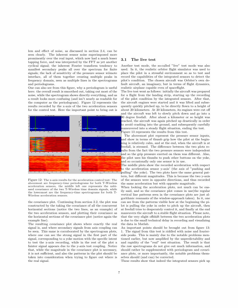
lem and effect of noise, as discussed in section 2.4, can beseen clearly. The inherent sensor noise superimposed moreprominently over the real input, which now had a much lessertapping force, and was interpreted by the FFT as yet anothercyclical signal; the inherent Fourier transform tendency tomanifest secondary peaks all over the spectrum for finitesignals; the lack of sensitivity of the pressure sensor wiimoteinterface, all of them together creating multiple peaks infrequency domain, seen as multiple lines in the spectrogramsand periodograms.One can also see from this figure, why a periodogram is usefulhere: the overall result is smoothed out, taking out most of thenoise, while the spectrogram shows directly everything, and asa result looks more confusing (and isn’t nearly as readable forthe computer as the periodogram). Figure 12 represents theresults recorded by the x-axis of the two acceleration sensorsfor the control test. Here the important point to bring out is

Figure 12: The x-axis results for the acceleration control test: Theabovemost are frequency-time periodograms for both T-Wirelessacceleration sensors, the middle left one represents the unbi-ased covariance of the two T-Wireless time domain signals, whilethe lowermost are the frequency-time spectrograms for both T-Wireless acceleration sensors.

the covariance plot. Continuing from section 2.2, the plot wasconstructed by the taking the covariance of all the concurrenthorizontal sections (notice the two lines, as an example) ofthe two acceleration sensors, and plotting their covariance asthe horizontal sections of the covariance plot (notice again theexample line).The resulting covariance plot shows where exactly the realsignal is, and where secondary signals from axis coupling canbe seen. This same is corraborated by the spectrogram plots,where one can see the strong signal in the first part of thesignal, corresponding to a yoke motion with the specific intentto test the x-axis recording, while in the rest of the plot afainter signal appears due to the y-axis test coupling. Noticethat, while the magnitude in the covariance plot is necessary,it is not sufficient, and also the patterns in the plot should betaken into consideration when trying to figure out where isthe real signal.

3.1 The live testAnother test mode, the so-called ”live” test mode was alsoused. In it, the realistic orbiter flight simulator was used toplace the pilot in a stressful environment so as to test andrecord the capabilities of the integrated sensors to detect thepilot’s condition. The chosen aircraft was Orbiter’s own de-fault aircraft, an imaginary, but in terms of flight dynamics,realistic airplane capable even of spaceflight.The live test went as follows: initially the aircraft was preparedfor a flight from the landing strip, starting up the recordingof the pilot condition by the integrated sensors. After that,the aircraft engines were started and it was lifted and subse-quently quickly pitched up, to be directly flown to a height ofabout 20 kilometers. At 20 kilometers, its engines were cut offand the aircraft was left to slowly pitch down and go into a90 degree freefall. After about a kilometer or so height wasreached, the aircraft was again pitched up drastically in orderto avoid crashing into the ground, and subsequently carefullymaneuvered into a steady flight situation, ending the test.Figure 13 represents the results from this test.

The abovemost plot represent the pressure sensor inputs,and show in terms of thumb grip how the pilot at the begin-ning is relatively calm, and at the end, when the aircraft is atfreefall, is stressed. The difference between the two plots re-sults from the fact the two pressure sensors were independentand so the grip pressure exerted on them was different. Also,the pilot uses his thumbs to push other buttons on the yoke,and so occasionally only one sensor is in use.The middle plots show the recorded acceleration with respectto the acceleration sensor y-axis’ (the axis of ”pushing andpulling” the yoke). The two plots have the same general pat-tern, but different magnitudes. This is because the two y-axisof the sensors were in opposite directions, and thus recordedthe same acceleration but with opposite magnitude.When looking the acceleration plots, not much can be eas-ily said, and so the covariance plot comes in use(the regularvertical line patterns seen in the covariance plots are just al-gorithmic remnants of the window-approach taken). In it, onecan see from the patterns visible how at the beginning the pi-lot is pulling the yoke in order to pitch up the aircraft, thenat freefall tries to desperately control it, and finally at the endmaneuvers the aircraft to a stable flight situation. Please note,that the very slight offshift between the two acceleration plotsis due to the small technical delay in recording and visualizingthe data in Matlab.An important points should be brought out from figure 13:1. The signal from this test is riddled with noise and fourier-side peaks. This is mainly due to the notable problems men-tioned earlier, but now amplified by the unpredictability andand rapidity of the ”real” test situation. The result is thatthe raw spectrograms do not give out much information, andshould rather be supplemented with periodogram and covari-ance plots, or more importantly, the notable problems them-selves should (and can) be corrected.These results show that indeed the integrated sensors pick up

7

Figure 13: The abovemost two plots are spectrograms for the pressure sensors ; the middle two represent the y-axis input from thetwo T-Wireless acceleration sensors; and the bottom two are the covariance plot for the two acceleration sensors, and a backup y-axisplot from the wiimote

and record the pilot input successfully, and with a bit more ad-justment and improvement, mainly in getting rid of the prob-lems mentioned in section 2.4, a clear enough signal can beachieved for the computer to read and interpret correctly.

4 Conclusions and recommendations

As the results point out, working integration of the grippressure and steering acceleration sensors was achieved.Further, it should be emphasized that all of the discussedanalysis methods can be done in real-time, online. The onlydifference that would have to implemented, would most likelyconsist of converting the Matlab code into a more run-timefaster computer language, such as C/C++, and other minorefficiency improvements.Other improvements could (and should) also be implemented:obviously more pressure sensors should be added to yokesystem, ideally covering as much as possible of its surface.Further on, the notable problems in section 2.4 shoulddefinitely be solved. Noise reduction has immediate andquite obvious advantages, and with due hardware selectionand modification, can be toned down to acceptable levels

(noise of course can never completely be eliminated). Intheory, noise can be effictely reduces during offline analysis,by recording its power spectral density during a no-inputmode, and subsequently subtracting that PSD from the mainsignal. This same procedure, however, is not as easy in onlinewith a constantly updating signal input and plot.More importantly, sensitivity should be increased as much aspossible in order to be able to detect clearly, combined withmore pressure sensors on the yoke, the pilot’s blood pressureand heart rate.The acceleration sensor’s axis’ should be uncoupled from eachother, mainly through clever placement of sensor’s referenceframe with respect to the main reference frame of the yoke,but more concretely, by reforming the yoke’s surface suchthat a sensor can be placed in a framewise correct positionand unobtrusively, and mathematical and physical modelling,correction and adjustment of the accelerations felt by thesensor in use.With the help of these improvements, much more (detailed)information on the pilot’s condition can be accessed, recordedand analysed, thus improving the system considerably. Theseimprovements are not difficult to implement, and in fact can

8

be considered to a natural next step in the development ofthis integrated system.Other, theoretical and mostly code-based improvementsinclude: An improved FFT algorithm, such as a GoertzelFFT Algorithm ; an improved Xpass filter, or even a wavelettransform-based filter.As mentioned in section 2.2, the FFT produces distractionssuch as extra peaks. Thus, a more appropriate FFT algorithmshould concentrate one the ”interesting” part of the spectrum,i.e. where one expects to find the signal in, which is exactlywhat the Goertzel version of the FFT algorithm is capable ofdoing.Further, improving the Xpass filter used, or instead usingcontinuous wavelet transform (CWT) techniques, couldpotentially reduce the noise involved considerably. CWTbasically scales down a continuous input signal into severaluser-definable ”daughter” signal, or wavelets, and can do thisfrequencywise. Thus a wavelet represents a part of the signalin a different portion of the spectrum, isolating the noisy partin one wavelet and the signal in another.

4.1 Future development

The next step, after the above mentioned improvements havebeen implemented, is to add a degree of intelligence. This isno longer part of the intended purpose of this work, but rathera recommendation on how it should be further developed.The main idea is to give ability to do not only analysis, butrudimentary decision-making capabilities as well. As criticalsituations in aerospace often appear and evolve in timescalestoo fast for a human operator, the ACS could be designated asthe decision-maker in that situation by creating an extra feed-back loop. Of course, the ACS would not take total control,but rather augment the pilot’s flight performance.The sensor data would have to be first processed in a in-between step, such as Matlab in this work, and transformedinto a format most suitable for the simulator/ACS. Obviouslythis suitable format would not be the raw data coming fromthe sensor, but rather the direct input coming from the stick( X(s) ), modified by a transfer function based on the sensorinput ( Y (s) = X(s)H(s) ).The function H(s) would be de-cided by the in-between computer based on some predefinedinstruction set or other decision making part, and would bechosen in such a way as to correct or enchance the perfor-mance of the pilot, for example by dampening any erratic ortwitching motion of the pilot input during landing.Figure 14 shows a functional flow on how the process works.An important thing to emphasize is that this work would onlybe a complementary part of the whole ACS system, and workcooperatively with the rest of the automatic functions. Forexample, during a landing of an aerospace vehicle and pushingthrough the operational flight envelope, the automated func-tions of the ACS usually constrict the pilot operation ( max.descent rate, height etc.), or at least give a warning, based onthe preset conditions in the ACS and triggered by the its abil-ity to sense the physical position and kinetics of the aircraft [8].

This work would then add another feedback loop and a sourceof information for the ACS, so that it has the ability to adjustits influence during flight according to the pilot input.

References

[1] M. M. van Paassen R., Human-machine interfaces inaerospace - lecture 1, Lecture notes, Technical Universityof Delft course Human-Machine interfaces in Aerospace.

[2] W. D. Christoffersen K., How to make automated systemsteam players, in Advances in human performance and cog-nitive engineering research, Volume 2, -, 2002.

[3] Current Status and Future Prospects of Aviation HumanFactors in Japan, last visited on December 8,2008.

[4] N. M., China airlines airbus a300-600r(flight 140)misses landing and goes up in flame at nagoya air-port, Failure Knowledge Database / 100 selected caseshttp://shippai.jst.go.jp/en/Search.

[5] A. R.R., Automation in aviation: A human factors per-spective, in Handbook of aviation human factors, LawrenceErlbaum Associates Inc., 1999.

[6] A. K. et. al., The interfaces between flightcrews and mod-ern flight deck systems, United States Federal AviationAdministration (FAA) - Human Factors Team, 1996.

[7] D. O. D., Molson medical informatics sampler,http://www.mmi.mcgill.ca/mmimediasampler2002/, lastvisited on December 8,2008.

[8] T. A. Handbook, Cary R. Spitzer (CRC Press, 2001), B-777 Design Philosophy.

9

(a) (b)

Figure 14: a) The main steps and components of the desired system with a second feedback loop, and b) the decisionmaker, in thiscase within the block ”Matlab”.

10