Gridlock and Ine¢ cient Policy Instruments1

David Austen-Smith

Kellogg School of Management, Northwestern University, USA

Wioletta Dziuda

Harris Public Policy, University of Chicago, USA

Bård Harstad

Department of Economics, University of Oslo, Norway

Antoine Loeper

Department of Economics, Carlos III University, Spain

January 29, 2019

1This paper has bene�ted from the comments of seminar participants at at Banco De Espana,Cerge-EI, Prague, Columbia University, Nottingham University, University of Oslo, Princeton Uni-versity, University of Rochester, Stanford University, and Washington University. In particular, weare grateful to Vincent Anesi, Dan Bernhardt, Alessandra Casella, Ying Chen, John Duggan, Tas-sos Kalandrakis, Navin Kartik, Carlo Prato, Daniel Seidmann, Michael Ting and Jan Zapal. DavidAusten-Smith is also grateful for support under the IDEX Chair, "Information, Deliberation andCollective Choice" at IAST, Toulouse. Antoine Loeper gratefully acknowledges the support fromthe Ministerio Economía y Competitividad (Spain), grants ECO-2016-75992-P , MDM 2014-0431,and Comunidad de Madrid, MadEco-CM (S2015/HUM-3444). Part of this research was conductedwhile Antoine Loeper was research fellow at Banco de Espana. All responsibility for any errors orviews herein, however, lies exclusively with the authors.

Abstract

Why do rational politicians choose ine¢ cient policy instruments? Environmental regulation,

for example, often takes the form of technology standards and quotas even when cost-e¤ective

Pigou taxes are available. To shed light on this puzzle, we present a stochastic game with

multiple legislative veto players and show that ine¢ cient policy instruments are politically

easier than e¢ cient instruments to repeal. Anticipating this, heterogeneous legislators agree

more readily on an ine¢ cient policy instrument. We describe when ine¢ cient instruments

are likely to be chosen, and predict that they are used more frequently in (moderately)

polarized political environments and in volatile economic environments. We show conditions

under which players strictly bene�t from the availability of the ine¢ cient instrument.

1 Introduction

Over the years, the economics profession has converged at a set of e¤ective policy recom-

mendations for a wide variety of policy areas. For example, there is widespread agreement

that externalities can be more e¢ ciently internalized with Pigou taxes than with command-

and-control interventions, and that it is less distortionary to increase public revenue by elim-

inating economically unjusti�ed tax deductions and exemptions than by raising tax rates.

Likewise, economists have argued that some �scal consolidation policies are less harmful

than others. In practice, however, these recommendations are frequently ignored. Instead,

policy makers often intervene with strictly less e¢ cient policy instruments than others that

are as readily available. This paper concerns why such apparently irrational (all else equal)

political decisions might arise in a world of instrumentally rational agents.

To understand this puzzle, we present a dynamic political economy model in which the

government reacts to external shocks by choosing a policy from a given menu of policies, one

of which is unequivocally Pareto dominated by another available alternative. Indeed, the

ine¢ cient policy is not only Pareto dominated by the alternative at the time of adoption,

but in all possible states of the world. Nevertheless, we show that the ine¢ cient policy

intervention can arise naturally from a simple legislative bargaining model without any

extraneous frictions or informational asymmetries: it is the very ine¢ ciency of the policy

that makes it appealing to legislators. We further show that the availability of an ine¢ cient

policy instrument, either in addition to or in place of an e¢ cient policy, may, at least in

equilibrium, improve the welfare of all policy makers.

Our legislative bargaining model rests on three characteristics. First, legislative policy

decisions involve two pivotal players. In particular, policy change requires the consent of

two veto players who may disagree on when to enact or repeal an intervention. Second, the

status quo policy in a dynamic, multi-period setting is endogenous: the policy implemented

in one period becomes the status quo in the next. Third, the environment is subject to

shocks across time that a¤ect the state-contingent policy preferences of the veto players in

any period, thereby creating the need for periodic renegotiations.

In a closely related model with only one available policy intervention, Dziuda and Loeper

(2016) observed that the three characteristics described above imply that the legislator who

is pivotal for introducing the intervention is distinct from the legislator pivotal for repealing

it. Consequently, the anticipation of her loss of political in�uence makes the legislator pivotal

for implementing the intervention less inclined to introduce it in the �rst place, fearing that

it will be hard to repeal should circumstances change. Loosely speaking, (Markov perfect)

equilibrium behavior involves political gridlock. In this paper, however, we show that when

1

players can choose not only whether, but also how, to intervene, the fear of future gridlock

can induce an ine¢ cient policy intervention: the veto player can agree on an ine¢ cient policy

instrument because the ine¢ cient instrument will be easier to repeal. As a result, there may

be states of nature in which the more economically e¢ cient intervention is not politically

feasible, whereas the less e¢ cient intervention is approved by both veto players.

In particular, we characterize conditions under which the ine¢ cient policy instrument is

implemented with positive probability in equilibrium. Intuitively, for an ine¢ cient policy

response to be chosen by rational legislators, it must be the case that the ine¢ ciency is

su¢ ciently high (respectively, low) for the more (respectively, less) interventionist legislator

to approve repealing the policy in some states, so that the ease of repeal o¤sets the cost of

ine¢ ciency for using the ine¢ cient policy in other states. For any strictly positive level of

ine¢ ciency, however, there exist nonpathological distributions of the state of nature under

which legislators use the ine¢ cient instrument in all equilibria.

The theory links both the political environment and the level of economic stability to the

choice of policy instrument. To see this, �x the level of economic stability and consider the

political environment. Suppose that the ideological distance between the legislators increases.

This increases gridlock, creating room for the use of easily repealable instruments. The re-

lationship between ideological polarization and the use of ine¢ cient instrument, however,

turns out to be non-monotonic in our framework. The relative ease of repealing ine¢ cient

policies makes such policies attractive interventions for moderate levels of ideological polar-

ization, but not when ideological polarization is small or when it is large. To see why, note

that when the veto players have su¢ ciently similar preferences, they are likely to agree on

when to repeal an e¢ cient intervention. Conversely, when their preferences are su¢ ciently

polarized, they are likely to disagree on when to repeal either type of policy intervention,

in which case the strategic bene�t of an ine¢ cient intervention is too small to outweigh its

cost.

To understand the e¤ect of economic volatility, �x the political environment. For stable

economic environments, the current state of nature changes little over time and any policy

intervention can be expected to persist for quite some time. Consequently, the expected cost

of intervening with an ine¢ cient instrument is larger than the option value of being able to

repeal such a policy more readily. On the other hand, if the current economic environment

is volatile, the state of nature can vary considerably and the possibility of at least one veto

player preferring to repeal an intervention relatively quickly can be high. The relative ease

with which ine¢ cient interventions are repealed, therefore, makes use of such instruments

attractive in this situation.

We show that all veto players can be strictly better o¤ in equilibrium if the ine¢ cient

2

intervention is available as a policy option. Hence, our paper not only o¤ers a rationale for the

use of ine¢ cient policy instruments, but also implies that they can be bene�cial given the

political constraints induced by a collective choice mechanism with multiple veto players.

The less interventionist player bene�ts from the availability of the ine¢ cient intervention

because it is easier to repeal, and the more interventionist player bene�ts because it makes

policy intervention politically feasible.

The model�s logic can be applied to a variety of settings, including infant industry pro-

tection, environmental regulation, �scal consolidation and �nancial regulation.

Temporary protection of infant industries. Trade theorists (see, e.g., Bardhan

1971) have argued that in the presence of dynamic learning externalities, protecting an infant

industry from foreign competition (or protecting an established industry from a temporary

surge in foreign competition) can raise social welfare. The literature has further shown that

subsidies are preferable to tari¤s because they do not distort consumption and, because of

the double-dividend e¤ect, that tari¤s are preferred to quotas and other non-tari¤ barriers

to trade. However, an important condition for these measures to be socially desirable is

that they must be repealed when the industry matures (or when the temporary increase in

foreign competition vanishes), although policy makers do not know ex-ante when that will

occur (Melitz 2005). The logic of our model suggests that the more free-trade oriented party

might prefer to protect the domestic industry with ine¢ cient non-tari¤ barriers to trade

for fear that the more protectionist party will veto a repeal of more e¢ cient protectionist

policies. In fact, since WWII, governments have increasingly relied on non-tari¤ barriers to

trade to adapt trade policies to changes in trade �ows (Bagwell and Staiger 1990).

Environmental regulation. Despite the sometimes considerable di¤erences in perspec-tive, economists from left to right tend to recommend Pigou taxes to regulate an external-

ity because they are cost-e¤ective, require little information, and o¤er a �double dividend�

whereby emission taxes generate public revenues that allow governments to reduce other dis-

tortionary taxes.1 It is thus �a mystery�, according to some economists, why the Republican

Party in the US blocked such a market-based policy during the Obama administration, since

doing so e¤ectively led to the command-and-control regulation of power plants introduced

by that administration in 2015.2 In line with our model, however, some key Republicans

1Following the seminal paper by Tullock (1967), there is now a large literature on the double divi-dend. For a recent survey, see Jorgensen et al. (2013). In part because of the double dividend, all butfour of �fty one prominent economists surveyed in 2011 agreed that a carbon tax would be the less expen-sive way to reduce carbon-dioxide emissions. (http://www.igmchicago.org/igm-economic-experts-panel/poll-results?SurveyID=SV_9Rezb430SESUA4Y)

2http://www.nytimes.com/2015/07/01/business/energy-environment/us-leaves-the-markets-out-in-the-�ght-against-carbon-emissions.html. While Pigou taxes are also relatively rare internationally, a famousexception is British Columbia, which introduced a carbon tax in 2008. Although initially controversial,

3

may have anticipated that the administration would impose some curbs on the energy sector

regardless, forcing them to use ine¢ cient (command-and-control) instruments that would

be easier to repeal once Obama�s term was completed.3 And, at the time of writing, the

Republican administration is indeed working to repeal the regulations. It is hard to envision

that the same attempt would occur if the intervention to be repealed was an e¢ cient carbon

tax combined with a lump-sum subsidy or a tax o¤set.

Fiscal consolidation. Consider a country deciding how to consolidate its �scal policyafter a shock has put its public debt on an unsustainable path. Although its government

can do so along a variety of policy dimensions, we illustrate the logic of our argument by

considering only one possibility, namely whether to focus on increasing revenues or decreasing

outlays. Suppose, as the existing empirical evidence suggests, that a spending cut is less

contractionary and thus statically preferred by the policy makers to a tax increase. In

that case, the less interventionist veto player is the veto player ideologically least inclined

to implement a spending cut, that is, the liberal veto player. Our theory suggests that

the liberal veto player may veto the spending cut and support instead a more costly tax

increase in anticipation that, once the �scal situation improves, it will be easier to convince

the conservative player to decrease taxes than to increase spending to its pre-crisis level.4

Consistent with this logic, there is empirical evidence indicating that �scal adjustments

based on spending cuts are longer-lived than �scal adjustments based on tax increases, i.e.,

the e¢ cient adjustment is more persistent than the ine¢ cient one (e.g., Alesina et al. 1998,

Alesina and Ardagna 2013).5

Financial regulation. Financial regulation tends to respond to �nancial crises. Forexample, after the �nancial crisis of 2007-2008, the U.S. Congress passed the Dodd-Frank

Wall Street Reform and Consumer Protection Act. Although hailed by many as a step in

the right direction, it is a complex piece of legislation that others consider ine¢ cient. Its

the tax has gained support from all important stakeholders thanks to the rebates in other taxes thatthe revenues permit (http://www.nytimes.com/2016/03/02/business/does-a-carbon-tax-work-ask-british-columbia.html?smid=pl-share&_r=0).

3Jim Manzi, a prominent conservative commentator on climate change, said openly that �a carbon taxwould be, mostly likely, a one-way door: Once we introduce it we�re stuck with it for a long time. What if oureconomic and climate models are too aggressive, and there is no practical economic justi�cation for emissionsreductions [. . . ] There are very large potential regrets to a carbon tax.�(In �Conservatives, Climate Change,and the Carbon Tax�, The New Atlantis, 2008 (21), 15-25)

4See Alesina et al. (2017) for a recent literature review. The �ndings of that literature are still subject tointense debate, but we would like to point out that the logic of our model applies equally to the opposite casein which a tax increase is more e¢ cient than a spending cut, the only di¤erence being that the interventionistplayer is then the liberal veto player.

5An alternative explanation for why tax hikes might be chosen even when they are less e¢ cient thanspending cuts is that the latter hurt powerful constituencies such as retirees or unions. However, thatexplanation is harder to reconcile with empirical �ndings that governments whose austerity programs focuson spending cuts are no less likely to be reelected than those who focus on tax increase (Alesina et al. 1998).

4

provisions rely on heavy government regulation instead of price instruments recognized as

more e¢ cient at curbing systemic risk. Applying the same lens here as for the environmental

regulation example, the ine¢ ciencies can be viewed as a price paid by liberals to insure at

least some regulation was implemented and, from the perspective of the more laissez faire

members of Congress at the time, an acceptable intervention in response to the fallout

from the crisis but one that can be more easily unpacked in economically calmer times.

Consistent with this view, on June 9 2017, The Financial Choice Act, legislation that would

�undo signi�cant parts�of Dodd-Frank, passed the House 233-186.

Related literature. We are not the �rst ones to o¤er an explanation for why gov-

ernments implement ine¢ cient policies. However, the logic that underlies our argument is,

to the best of our knowledge, novel: ine¢ cient interventions are more likely to be repealed

should circumstances change, making them more likely to be accepted in the �rst place by

all veto players. On the abstract level, there are three main features that distinguish our

paper from the literature. First, the mechanism does not depend on the speci�cities of the

economic environment, or on how the policy interacts with the private sector or the elec-

torate. Instead, ine¢ ciency arises solely from the con�ict of interests between legislators and

the need to adapt the policy to a changing environment. Second, the ine¢ cient policy in

our model is ine¢ cient in a static sense: there exists a policy that gives a strictly greater

�ow payo¤ to all relevant decision makers in all states of nature. Third, the ine¢ cient policy

is not only the result of status quo inertia whereby a previously optimal policy becomes

obsolete. Instead, it is actively implemented by the policy makers.

The paper closest to ours is Dziuda and Loeper (2016), who analyze a similar model

except that they restrict the policy set to policies that are statically Pareto undominated

for some states. They show that ine¢ cient inertia occurs because each pivotal player fears

that policy changes approved by her will be hard to repeal when she wishes to do so. As

a result, the status quo can persist even when Pareto dominated. Hence, any ine¢ ciency

takes form of status quo inertia and any policy change is a Pareto improvement. Riboni and

Ruge-Murcia (2008), Zapal (2011), Duggan and Kalandrakis (2012), Bowen et. al. (2017),

and Dziuda and Loeper (2018) consider related models of dynamic legislative bargaining

which also lead to policy inertia. Relative to these papers, our contribution is to show that

adding a Pareto ine¢ cient alternative to the policy space can mitigate policy inertia. In

particular, legislators may adopt a Pareto-dominated policy change.6

6In a distributive environment, Bowen et. al. (2014) and Anesi and Seidmann (2015) show that endoge-nous status quo can lead to Pareto ine¢ cient policies, because they allow the proposer or the supportingcoalition to extract greater transfers in the future. In these papers, preferences do not evolve over time, asin most of the literature on dynamic policy making with an endogenous status quo. Policy dynamics occurbecause the proposer changes (e.g., Baron 1996, Bernheim, Rangel and Rayo 2006, Kalandrakis 2004, Anesi

5

Since our model requires policy makers to respond to shocks, it is related to the literature

on policy reforms. Alesina and Drazen (1991) show that legislators can engage in war

of attrition over who should bear the costs of reform. Fernandez and Rodrik (1991) and

Ali, Mihm and Siga (2017) show that uncertainty over the distributional impact of reforms

may sti�e them. Spolaore (2004) compares the likelihood of policy adjustment across three

stylized institutions. In Strulovici (2010), an endogenous status-quo bias arises if a majority

learns that the new policy is bene�cial for them. Anticipating this situation, policy makers

may not want to try out new policies in the �rst place. Unlike in our model, these papers

consider the policy response to a single shock after which legislators�policy preferences are

�xed over time and restrict attention to e¢ cient policy adjustments. Hence, ine¢ ciency only

takes the form of delays or failure to intervene. In contrast, legislators act without delay in

our model but the solution they adopt is ine¢ cient.

There is also large political science literature that explores ine¢ cient policy making due

to structural characteristics of legislative decisionmaking (e.g., the �libuster or committee

structure). Important examples here include Krehbiel (1998) and Brady and Volden (2006),

who explore models of gridlock, Ortner (2017), who shows that gridlock is likely near the

next election, and Weingast, Shepsle and Johnson (1981) and Cox and McCubbins (2000),

who analyze legislative structure and ine¢ cient public good provision more generally. To our

knowledge, however, there is as yet no analysis focusing directly on the deliberate strategic

choice of ine¢ cient policy change when policy change occurs.

Ine¢ cient policy choices by a unitary actor, whether a single legislator or a fully coordi-

nated party or group, can be also explained by aspects of the political economic environment

other than legislative design. In Coate and Morris (1995), Acemoglu and Robinson (2001),

and to some extent Glaeser and Ponzetto (2014), ine¢ cient policy choices arise from an

incumbent legislator�s e¤orts to retain o¢ ce.7 Whereas the Coate and Morris (1995) and

Glaeser and Ponzetto (2014) accounts rest on asymmetric information, Acemoglu and Robin-

son (2001) generate policy ine¢ ciency from a model in which distortionary transfer payments

are designed to counter declining political support and in�uence. Tullock (1993), Grossman

and Duggan 2017, Buisseret and Bernhardt 2017), or because the same proposer forms di¤erent coalitionsover time (e.g., Diermeier and Fong 2011). In contrast, in our model, each proposer always seeks the supportof the same policy maker and the qualitative nature of policy ine¢ ciencies is, by and large, independent ofthe allocation of bargaining power. Acharya and Ortner (2013) obtain Pareto ine¢ cient solution in a divide-a-dollar game because, as in our paper, players cannot commit to trade-o¤ their payo¤s intertemporally. forsimilar reason as ours: A di¤erent strand of literature assumes that the implemented policy in�uences futurestates (see Hassler et al., 2003, for example). Baldursson and Von Der Fehr (2007) is closer to our story,as they argue that a relatively �brown�party may prefer quotas rather than taxes, because the relativelyine¢ cient quotas are essentially property rights that are di¢ cult to tighten or remove later.

7See also Canes-Wrone, Herron and Shotts (2001) and Buisseret and Bernhardt (2018) for how electoralincentives can lead to policy distortions.

6

and Helpman (1994), Becker and Mulligan (2003) and Drazen and Limao (2008) argue that

any resource transfer increases wasteful lobbying (rent-seeking) activity. By committing it-

self to ine¢ cient transfers, the government can reduce the level of wasteful lobbying. More

generally, there is an extensive literature on policy distortions induced through special inter-

est groups�lobbying and campaign contribution activities (see Wright 1996 and Grossman

and Helpman 2001 for overviews of the literature)

The problem at the root of our paper is related to the dynamic lack of commitment

studied extensively in the literature. In Acemoglu and Robinson (2000, 2001) or Fearon

(1998), for example, the inability of the players to commit leads to ine¢ cient con�ict (see

Powell, 2004, for an interesting overview). In our paper, the inability of the players to

commit to a repeal of certain policies lead to Pareto ine¢ cient gridlock. Giving players

access to Pareto ine¢ cient alternatives that they frequently may want to repeal due to their

ine¢ ciency can mitigate this commitment problem.

Aidt (2003) claims that ine¢ cient command-and-control instruments are more bureau-

cracy intensive and, to the extent that bureaucrats in�uence policy design and derive value

from implementing policy, such interventions are favored by bureaucrats. Alesina and Pas-

sarelli (2014) and Masciandaro and Passarelli (2013) o¤er explanations of socially suboptimal

policies that hinge on the median voter failing to internalize the costs and bene�ts to oth-

ers when policies have di¤erent distributional consequences. However, both available policy

choices are Pareto optimal in these papers. In contrast to these approaches, ine¢ ciency in

our model does not depend on groups, informational asymmetries, or reelection concerns.

2 A Simple Example

In this section we present a stylized example to illustrate the key mechanism and to preview

some of our results. The mechanism requires two pivotal players, or legislators, L and R,

both of whom must approve any policy change. Speci�cally, at the start of any legislative

period, nature randomly chooses one legislator to propose a change in, or maintain, the status

quo policy. The other legislator has a veto right over any proposed change in the status quo.

Legislators start with no intervention, denoted by n; and can intervene by introducing either

an e¢ cient instrument p or an ine¢ cient instrument q: The �ow-payo¤ from policy n is

normalized at 0: Intervention gives everyone a bene�t �, and the costs associated with p and

q are wi and wi + ei, respectively, for i 2 fL;Rg. We assume that ei > 0 for each i, so thatei is the additional bene�t of the e¢ cient instrument.

We can immediately make some simple observations:

Proposition 0 Suppose there is only one period. Then the ine¢ cient policy q is never

7

implemented in equilibrium.

Suppose now that there are two periods and let � > 0 be the common discount factor.

The status quo in the �rst period is n and the �rst-period policy becomes the status quo

in the second period. Assume further that there are only two states, � and �� > �; with ��

occurring with probability �, and suppose that the costs associated with p and q satisfy

wL < � < minfwL + eL; wRg � maxfwL + eL; wR + eRg < ��: (1)

The last inequality in (1) means that in state ��; both players prefer any type of intervention

to n. The �rst two inequalities in (1), however, imply that in state �, the less interventionist

player R prefers no intervention, while the more interventionist player L prefers to intervene

but only if the intervention is with the e¢ cient instrument. In terms of our environmental

application, �� can be interpreted as the usual state of the economy in which both parties agree

that environmental interventions are desirable, while � can be interpreted as an economic

downturn that makes the R party (but not the L party) want to repeal any regulation that

can compromise economic growth. In the case of �scal consolidation, � may be interpreted

as a business-as-usual state in which parties di¤er ideologically on whether public spending

should be cut, while �� can be interpreted as a �scal crisis state in which both parties are

willing either to cut spending or to increase taxes to bring public debt under control.

Consider the last period in this game. In state ��, both players strictly prefer p to any

other policy. So, independently of which player has proposal rights, p is implemented in that

state. What is implemented in the low state �, however, depends on the status quo. If n

is the status quo, R does not approve (propose or accept, depending on the allocation of

proposal rights) any change in policy. Similarly, if p is the status quo, L does not approve of

any change in policy. Finally, if q is the status quo, then the two players agree that either n

or p are better than the status quo, but they disagree on which is best. In this situation, p

is implemented if L has the proposal power and n is implemented otherwise. This reasoning

implies that, in the second period, p is not repealable, but q can be repealable when the

realized state in that period is �.

Consider now the �rst period, and suppose the state is �� with status quo n. Both players�

�rst period �ow-payo¤s are maximized by policy p: But since p is not repealable, R may be

reluctant to approve such a change in policy. In particular, R does not approve p in the �rst

period if the bene�t of p relative to n in state �� is outweighed by the expected cost of being

stuck with p in state �; that is, if:

� � wR < � (1� �) (wR � �) : (2)

8

Thus, players fail to intervene e¢ ciently in the �rst period if the disagreement state � is

relatively likely (i.e., 1�� is high), if players are patient, and if R�s preference for interventionin state � is relatively weak compared to R�s preference for no intervention in state �. On the

other hand, because q is more easily repealed than p, R may be willing to intervene with q:

Denoting by bL 2 [0; 1] the probability that L has the authority to make a take-it-or-leave-itpolicy proposal in the second period, R approves an intervention q in the �rst period if

�� � wR � eR � � (1� �) bL (wR � �) : (3)

And since L receives a higher �ow-payo¤ from q than n in state ��, and the likelihood that a

change from status quo q to p in the second period exceeds that from n to p, L also prefers

and approves q over n in the �rst period. Finally, because players�share the same ordinal

policy preferences over n and q in both states, we have the following proposition.

Proposition 1 Suppose there are two periods and

� (1� �) bL (wR � �) + eR � � � wR < � (1� �) (wR � �) :

Then, in the �rst period of any subgame perfect equilibrium,

(i) intervention occurs in �� when the policy menu is fn; p; qg but not when the menu is fn; pg;(ii) both players strictly prefer menu fn; p; qg to menu fn; pg.

The fact that e¢ cient policies are hard to repeal can make them politically impossible

to agree upon in a dynamic setting. At the same time, as part (i) of the proposition states,

it is precisely because of its ine¢ ciency that both legislators may approve a �rst period

intervention with q in state �. And, as part (ii) of the proposition asserts, adding this

statically Pareto-dominated choice to the policy menu may not only result in its use, but it

also strictly improves equilibrium payo¤s for both players.

To our knowledge, the preceding claims are new to the literature. They are, however,

derived in a stylized example that raises a number of questions. For instance, the cost of

instrument q is limited since q will always be replaced by either n or p in the last period. But

what is the desirability of q in a dynamic model when there is no last period? Furthermore,

the binary state space in the example implies that instrument p will never be repealed once

implemented. But why should the players prefer q to p in a more general setting where both

interventions may eventually be repealed? To explore these and several other issues further,

the following section generalizes the model to an in�nite number of periods and to more

general distributions of states.

9

3 Model

Policies, payo¤s, and players. Two in�nitely lived players, L and R, must decide in eachperiod t 2 N which of three policies fn; p; qg to implement. Their preferences over thesepolicies in a given period t depend on the realization of the state of nature �(t) 2 R; and arespeci�ed as in the preceding example. That is, normalizing both players��ow-payo¤ from

policy n in any state � to zero, Ui(�; n) = 0, i 2 fL;Rg, player i�s �ow-payo¤ from policies

p and q relative to policy n in � are, respectively,

Ui (�; p) = � � wi; (4)

Ui (�; q) = � � (wi + ei).

Thus, ei is the period �ow-payo¤ gain for player i from implementing p instead of q. For

simplicity, we assume this gain is independent of �. More importantly, we assume that

ei > 0 for both players. That is, intervention p Pareto dominates intervention q in all states

of nature. Although the state of nature does not a¤ect which intervention is best, it a¤ects

whether an intervention is needed in the �rst place: given the zero �ow-payo¤ from no

intervention, n, player i gets a greater �ow-payo¤ from policy p than from policy n when

� � wi, and a greater �ow-payo¤ from q than from n when � � wi + ei. Importantly, unlesswe specify otherwise, we assume that wL 6= wR; that is, in some states of nature, players

disagree whether the e¢ cient intervention p is preferred to no intervention n. By convention,

L denotes the more interventionist player, so wL < wR.8 At times, we refer to wR � wL aspolarization over e¢ cient intervention.

Timing of the game. Every period t 2 N starts with some status quo s(t) 2 fn; p; qg,with s(0) = n. At the beginning of period t, both players observe the state �(t) 2 R.After �(t) is observed, L and R must collectively choose a policy from the set fn; p; qg. Weassume that one player makes a take-it-or-leave-it o¤er to the other regarding which policy

to implement. The recognition probability for player i is denoted by bi (�; s) ; which may

depend on the current state � and status quo s. We assume that bi is bounded below by

some b > 0: The recognized proposer o¤ers a policy y (t) 2 fn; p; qg . If the other player, theveto-player, accepts this proposal, then y(t) is implemented; otherwise, the status quo s (t)

stays in place. The policy implemented in t, whether the proposal y(t) or the status quo

s (t), generates the �ow-payo¤ for that period, as speci�ed in (4), and becomes the status

8The terms �instrument� and �intervention� are used exclusively in reference to alternatives p and q.The term �policy�may refer to any of the available alternatives, including n. This looseness should causeno confusion. Also, we say that a policy p or q is �repealed�when it is the status quo and players agree toreplace it by n:

10

quo in the next period, t + 1. Each player maximizes her expected discounted payo¤ over

the in�nite horizon. The common discount factor is � 2 (0; 1). For simplicity, we initiallyassume that f�(t) : t � 0g is distributed identically and independently over time accordingto some continuous c.d.f. F with full support. This assumption is relaxed in section 5 to

permit serial correlation.

Equilibrium concept. We denote the above game by � and restrict attention to

Markov-perfect equilibria, referred to as �equilibria� in what follows. A Markov-perfect

equilibrium is a subgame-perfect equilibrium in which players use Markov strategies. In this

game, a strategy is Markov if it depends only on the current state, the current status quo,

the identity of the proposer, and the current proposal at the action node of the veto player.

Let �i denote i�s Markov strategy. A (pure) Markov strategy for player i 2 fL;Rg consists oftwo contingent actions: a function that maps the current state and status quo into a policy

proposal, conditional on i being the proposer, and a function that maps the current state,

status quo, and proposal into a choice over accepting or rejecting the proposal, conditional

on i being the veto-player.9 Let � = (�L; �R). We brie�y discuss the robustness of our

restriction to Markov strategies at the end of Section 4.3. We allow for mixed strategies.

Since our interest regards the use of the ine¢ cient instrument q, throughout the paper

we focus on the equilibria in which q is implemented. To this end, the following de�nition is

useful.

De�nition 1 Let � be an equilibrium of �. Then, � is an instrument ine¢ cient equi-librium (IE) if q is implemented with positive probability on the equilibrium path; � is an

instrument e¢ cient equilibrium (EE) otherwise.

Remarks on the assumptions. Some of the assumptions are made for simplicity andrelaxing themmay not change the results. In particular, binary policy levels are not necessary

for the results. To see this, suppose that players can choose any level of p or q and consider

a two-period example again. The ine¢ cient instrument q will not be used in the last period

and the set of states under which p is repealed will be independent of its level. The ine¢ cient

q, however, will still be easier to repeal at any level, and the logic of our paper applies.

Three assumptions are crucial. First, the mechanics of the model rests on multiple veto

players. With a unicameral legislature taking decision under simple majority rule, the policy

maker i with the median wi would be the unique pivotal decision maker. However, multiple

9Note that Markov strategies are not allowed to depend on calendar time as the date is payo¤ irrelevantwith an in�nite horizon. Mixed strategies are admissible. More formally, writing �S for the set of probabilitydistributions over a set S, i�s proposal strategy takes R�fn; q; pg into � fn; q; pg; and i�s veto strategy takesR�fn; q; pg2 into � faccept; rejectg. Markov strategies are standard in the literature on dynamic bargainingwith endogenous status quo.

11

veto players are natural in politics. Bicameralism, supermajority requirements, presidential

veto power, or powerful interests groups imply the existence of a set of veto-players, or

pivots, whose approval is necessary and su¢ cient to enact a policy change. In the case of

a unicameral legislature taking decisions under a quali�ed majority m 2�12; 1�, player L is

such that exactly a fraction m of the wi�s are larger than wL and, for player R, exactly m

of the wi�s are smaller than wR. Thus, the degree of polarization wR � wL increases in themajority requirement m.

Second, we assume away explicit side-payments and state-contingent contracts. If the

players could make unlimited side-payments or sign state-contingent contracts, then only

e¢ cient policies would be implemented in equilibrium.10 In particular, policy p would be

implemented when � > (wL + wR) =2, and policy n would be implemented otherwise. Explicit

side payments and state contingent contracts, however, are rare and often unavailable in

politics. An important reason for this is that there is no independent third party that can

verify a particular realization of the state and enforce any ex ante agreement. In the case

of �scal consolidation, for example, � may capture the impact of a shock to money markets

on the long term sustainability of public debt and whether �scal consolidation can bring

this debt under control. Similarly, in the environmental application, � may capture changes

in the social cost of the polluting activity and the social opportunity cost of regulating the

polluting industry. And in the infant industry case, � might be the impact of a technical

innovation that a¤ects where an infant industry stands on its learning curve. In all of these

applications, it is unlikely that � could be measured in a transparent way by a nonpartisan

entity. Imperfect veri�able proxies for � may exist, (e.g., interest rate on government bonds

as a proxy for the impact of a shock to money markets), but whether and under what

conditions contracts contingent on such proxies improve the e¢ ciency of the policy making

is left for future research.

Third, we assume that any implemented policy stays in place until it is actively changed.

This is consistent with legislative practice. Most laws and policies enacted by the U.S.

Congress, for example, are permanent: they remain in e¤ect until a new legislative action

is taken. This is the case for mandatory spending policies, which include all entitlements,

currently about 60% of total federal spending (Austin and Levit 2010), constitutional amend-

ments, most statutes in the U.S. code, the Senate�s rules of proceedings, and international

treaties. Likewise, changes to the tax code are permanent unless legislators decide to attach

a sunset provision, that is, a clause that speci�es a period after which the relevant legislative

act automatically expires. Historically, attaching sunset clauses to legislation has been the

10For results on the e¢ ciency of state-contingent policies for the allocation of public goods, see Bowen etal. (2017).

12

exception rather than the norm, and tends to occur mainly for procedural reasons.11 Never-

theless, in theory, a sunset clause can address the concern of the less interventionist player

that an e¢ cient intervention will stay too long in place. Thus, the availability of sunset

clauses seems, at least prima facie, to remove the strategic value of ine¢ cient instruments

highlighted in this paper. In the working paper version, however, we present an example

that shows that even when sunsets are available at no cost, the ine¢ cient instrument might

still be implemented. A careful analysis of sunsets is beyond the scope of this paper.

4 Analysis

The following lemma states that an equilibrium exists, and that all equilibria have a relatively

simple structure: in any equilibrium of �; players behave as if they were playing a static

version of the game � (a single period) with �ow-payo¤ parameters (w�L; w�R; e

�L; e

�R) rather

than (wL; wR; eL; eR).

Lemma 1 There exist equilibria in �. Moreover, for any equilibrium �, there exists a uniquetuple (w�L; w

�R; e

�L; e

�R) 2 R4 such that the behavior prescribed by � is the same as the behavior

prescribed by an equilibrium of the game in which players play a single period of � with

payo¤s V �i (�; n) = 0 andV �i (�; p) = � � w�i ,

V �i (�; q) = � � (w�i + e�i ).(5)

All proofs are in the Appendix.12 We call (w�L; w�R; e

�L; e

�R) the continuation payo¤parameters

induced by � and note that they re�ect players� strategic preferences in the equilibrium,

that is, their policy preferences given continuation play �; as distinct from their exogenous

�ideological�preference parameters (wL; wR; eL; eR). Note that V �i (�; p)� V �i (�; q) = e�i ; soe�i represents the continuation payo¤ di¤erence for player i from some period t onward from

11See, e.g., Posner and Verneule (2002, pages 1672, 1694, and 1701) on the permanent nature of statutes,the Senate�s internal rules, or international treaties. As for tax legislation, prior to the Bush administration,the use of sunsets for changes in the tax code applied mainly to relatively small provisions known as �taxextenders�and were of signi�cantly smaller scale (Gale and Orszag 2003; Mooney 2004). Many sunsettedlegislations are frequently extended beyond the initial duration, often because of the activities of vestedinterests or the legislative costs of implementing the change. Since the repeal of ine¢ cient instrumentsrequires legislative work only when the state of nature justi�es it, and not at predetermined state-independentdates, using ine¢ cient instruments results in lower legislative cost than sunset provisions.12Duggan and Kalandrakis (2012) provide a very general existence result for dynamic bargaining games

with an endogenous status quo. But to apply their result directly here requires violating our assumption thatU(�; p) � U(�; q) is constant in �. Although introducing some noise to the payo¤s, to ensure the di¤erenceis not locally constant, and letting that noise tend to zero is possible, the result would be a correlatedequilibrium that obscures the particular tradeo¤s of interest here.

13

implementing p instead of q in that period, given continuation play �. Hence, e�i re�ects i�s

preferences over the e¢ cient and the ine¢ cient intervention in the dynamic game.

To understand the intuition for Lemma 1, consider the continuation payo¤gain for player

i from implementing p instead of n in some t. Player i gets a �ow payo¤ gain of �(t) � wiin period t, plus the expected continuation payo¤ gain from having status quo p instead

of n in t + 1. Since f�(t) : t 2 Ng is i.i.d., this expected continuation payo¤ gain does notdepend on �(t), but only on the anticipated play �, and hence is simply a constant C�. The

continuation payo¤ gain from implementing p instead of n in t is therefore �(t) � wi + C�;so w�i is given by wi � C�.13

The main goal of this paper is to understand the strategic underpinnings of IE and why

they can be bene�cial. Therefore, for the sake of exposition, we focus only on IE. We �rst

derive their properties (Section 4.1) and then the conditions under which they exist (Section

4.2).

Before we proceed, however, let us say a few words about the EE. By de�nition, in

any EE, the ine¢ cient instrument is not used; hence, EE are essentially equivalent to the

equilibria of the two-alternative game of Dziuda and Loeper (2016). They show that in

such equilibria, the more pro-intervention player distorts her votes in favor of p, and the less

pro-intervention player distorts her votes in favor of n, that is, w�L < wL < wR < w�R: As a

result, even EE are ine¢ cient in that there is excessive status quo inertia: a policy that was

once adequate for the environment becomes obsolete, but players do not agree to change it.

This kind of ine¢ ciency, however, does not explain the puzzle outlined in the introduction,

namely, why interventions that are ine¢ cient in any state of the world are implemented. So

IE di¤er from EE not in whether the equilibrium path is ine¢ cient, but in the nature of

ine¢ ciency.

4.1 Properties of IE

The following proposition summarizes the main qualitative properties of any IE.

Proposition 2 Let � be an IE. Then the corresponding continuation payo¤ parameters(w�L; w

�R; e

�L; e

�R) satisfy the following inequalities for some i; j 2 fL;Rg, i 6= j:

(i) the set of states at which j prefers to intervene with p is a proper subset of those at which

13If the process f�(t) : t 2 Ng is serially correlated, C� becomes a function of �(t) whose variations dependboth on the nature of the serial correlation, and on the set of types for which status quo n and p lead todi¤erent outcomes on the path of �. In particular, the continuation payo¤ gain from implementing p insteadof n, i.e., �(t) � wi + C� (�(t)) ; might become nonmonotone in �(t); possibly leading to equilibria that arenot in threshold strategies.

14

i prefers to intervene with p:

w�i < w�j ;

(ii) i prefers to intervene with p rather than q, and j weakly prefers to intervene with q rather

than p:

e�i > 0 and e�j � 0;

(iii) the set of states at which both i and j prefer to repeal p is a proper subset of those at

which they both prefer to repeal q:

mink2fL;Rg

(w�k ) < mink2fL;Rg

(w�k + e�k) :

Part (i) of Proposition 2 states that in any IE, one player i 2 fL;Rg is strictly moreinterventionist than the other player j. Part (ii) states that, in equilibrium, players disagree

on the appropriate intervention. In all states, player i prefers using the e¢ cient instrument

p to the ine¢ cient one q, whereas player j weakly prefers intervening with q rather than p.

Finally, part (iii) implies that, consistent with the intuition provided in the Introduction,

the ine¢ cient instrument q is easier to repeal than the e¢ cient instrument p. To see this,

assume p is the status quo. Then e�i > 0 implies player i always vetoes proposal q; and, by

de�nition of w�k , at least one player vetoes the proposal n for all states abovemink2fL;Rg (w�k ) :

Hence, in all such states, the status quo p remains in place. Conversely, for all states below

mink2fL;Rg (w�k ) ; both players prefer n to any instrument, so p is repealed. Both players,

however, prefer n to q in all states below mink2fL;Rg (w�k + e

�k). So (iii) implies that q is

repealed on a larger set of states than is p.

To understand the policy dynamics implied by Lemma 1 and Proposition 2, let us consider

�rst the equilibria in which e�j < 0; that is, equilibria in which j strictly prefers to intervene

with the ine¢ cient instrument. In that case, there are only two possible equilibrium paths,

illustrated by Figures 1 and 2 below, depending on whether maxkfw�k + e�kg < w�j (Figure 1)or w�j < maxkfw�k + e�kg (Figure 2). For concreteness, in Figures 1 and 2 we illustrate thesetwo possibilities for the equilibria in which i = L and j = R.14 States are measured along

the horizontal axis and policies are indicated by the three shaded bars above this axis. An

arrow identi�es an equilibrium policy change, conditional on the status quo, for any realized

state within the same interval of states as that in which the arrow is drawn. For intervals

of states where there is no arrow drawn, there is no policy change on the equilibrium path.

14Since wL < wR; it is natural to conjecture that necessarily i = L, but equilibria with i = R may arise aswell. See the discussion at the end of this section.

15

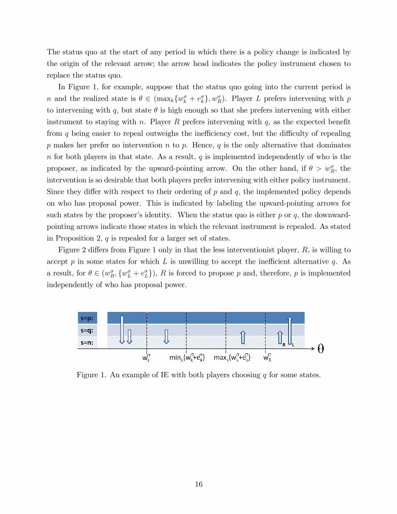
The status quo at the start of any period in which there is a policy change is indicated by

the origin of the relevant arrow; the arrow head indicates the policy instrument chosen to

replace the status quo.

In Figure 1, for example, suppose that the status quo going into the current period is

n and the realized state is � 2 (maxkfw�k + e�kg; w�R). Player L prefers intervening with pto intervening with q, but state � is high enough so that she prefers intervening with either

instrument to staying with n. Player R prefers intervening with q, as the expected bene�t

from q being easier to repeal outweighs the ine¢ ciency cost, but the di¢ culty of repealing

p makes her prefer no intervention n to p. Hence, q is the only alternative that dominates

n for both players in that state. As a result, q is implemented independently of who is the

proposer, as indicated by the upward-pointing arrow. On the other hand, if � > w�R, the

intervention is so desirable that both players prefer intervening with either policy instrument.

Since they di¤er with respect to their ordering of p and q, the implemented policy depends

on who has proposal power. This is indicated by labeling the upward-pointing arrows for

such states by the proposer�s identity. When the status quo is either p or q; the downward-

pointing arrows indicate those states in which the relevant instrument is repealed. As stated

in Proposition 2, q is repealed for a larger set of states.

Figure 2 di¤ers from Figure 1 only in that the less interventionist player, R, is willing to

accept p in some states for which L is unwilling to accept the ine¢ cient alternative q. As

a result, for � 2 (w�R; fw�L + e�Lg), R is forced to propose p and, therefore, p is implementedindependently of who has proposal power.

Figure 1. An example of IE with both players choosing q for some states.

16

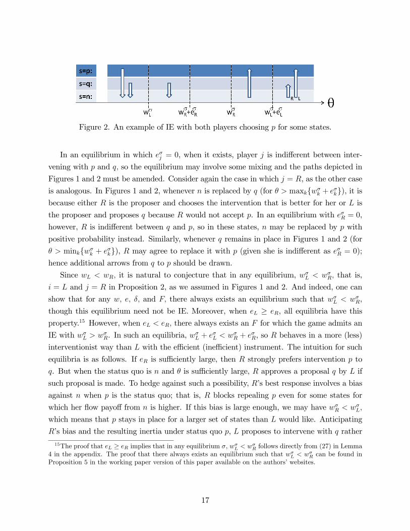
Figure 2. An example of IE with both players choosing p for some states.

In an equilibrium in which e�j = 0, when it exists, player j is indi¤erent between inter-

vening with p and q; so the equilibrium may involve some mixing and the paths depicted in

Figures 1 and 2 must be amended. Consider again the case in which j = R, as the other case

is analogous. In Figures 1 and 2, whenever n is replaced by q (for � > maxkfw�k + e�kg), it isbecause either R is the proposer and chooses the intervention that is better for her or L is

the proposer and proposes q because R would not accept p. In an equilibrium with e�R = 0,

however, R is indi¤erent between q and p, so in these states, n may be replaced by p with

positive probability instead. Similarly, whenever q remains in place in Figures 1 and 2 (for

� > minkfw�k + e�kg), R may agree to replace it with p (given she is indi¤erent as e�R = 0);hence additional arrows from q to p should be drawn.

Since wL < wR; it is natural to conjecture that in any equilibrium, w�L < w�R; that is,

i = L and j = R in Proposition 2, as we assumed in Figures 1 and 2. And indeed, one can

show that for any w; e; �; and F; there always exists an equilibrium such that w�L < w�R,

though this equilibrium need not be IE. Moreover, when eL � eR, all equilibria have this

property.15 However, when eL < eR; there always exists an F for which the game admits an

IE with w�L > w�R. In such an equilibria, w

�L + e

�L < w

�R + e

�R, so R behaves in a more (less)

interventionist way than L with the e¢ cient (ine¢ cient) instrument. The intuition for such

equilibria is as follows. If eR is su¢ ciently large, then R strongly prefers intervention p to

q. But when the status quo is n and � is su¢ ciently large, R approves a proposal q by L if

such proposal is made. To hedge against such a possibility, R�s best response involves a bias

against n when p is the status quo; that is, R blocks repealing p even for some states for

which her �ow payo¤ from n is higher. If this bias is large enough, we may have w�R < w�L;

which means that p stays in place for a larger set of states than L would like. Anticipating

R�s bias and the resulting inertia under status quo p, L proposes to intervene with q rather

15The proof that eL � eR implies that in any equilibrium �; w�L < w�R follows directly from (27) in Lemma4 in the appendix. The proof that there always exists an equilibrium such that w�L < w

�R can be found in

Proposition 5 in the working paper version of this paper available on the authors�websites.

17

than with p when the status quo is n, rationalizing R�s best response bias.16

4.2 Use of Ine¢ cient Instruments in Equilibrium

In this section we discuss how the types of equilibria and the equilibrium parameters (w�; e�)

vary with the primitives of the model. To understand the discussion below, recall that

from Proposition 2, an IE requires e�j � 0 for some player j; where e�j is j�s continuation

payo¤ di¤erence from a given period t onward from implementing p instead of q in t, given

continuation play �. Policy p yields a greater �ow-payo¤ than q in t, but status quo p and q

may also induce di¤erent continuation policy paths in t + 1. As illustrated in Figure 1 and

2, in t + 1; either status quo p and q are both repealed (for � small enough), in which case

they lead to the same continuation path, or they both stay in place (for � large enough), in

which case players keep on getting a greater �ow-payo¤ from p than from q, or status quo p

stays in place whereas q is repealed (for intermediate values of �), in which case the player

j who wants to repeal p in such states gets a greater continuation payo¤ from status quo

q. Thus, for e�j to be negative, the third case must be su¢ ciently likely and bene�cial to j;

relative to the ine¢ ciency of q.

Let us �rst discuss how the existence of IE depends on the degree of players�polarization

over when to enact and repeal p, as captured by (wL; wR). Fix F and �; and for simplicity,

consider the case eL = eR = e for some �xed e > 0; that is, q is equally ine¢ cient for

L and R: In that case, as discussed in Section 4.1, in any equilibrium, w�L < w�R; so from

Proposition 2, an IE requires e�R � 0: In the extreme case of no polarization wL = wR, playersdo not expect any disagreement, and the ine¢ cient instrument q has no strategic value. As

a result, the only equilibrium is an EE in which players behave as if they were playing a

one-shot game, i.e., w�L = w�R = wL = wR and e

�L = e

�R = e (see part (iii) of Proposition 3).

17

As players become more polarized (i.e., as wR increases and wL decreases), players�period

16In the appendix (see Example in Appendix 8.4), we consider and environment in which wL = wR andeL < eR and construct an IE � such that w�R < w

�L+e

�L < w

�R+e

�R < w

�R. By continuity, for some wL < wR;

there exists a near-by IE whose continuation payo¤ parameters satisfy the same inequality, which formallyproves that there exists an IE in which the more interventionist player behaves as the least interventionistin equilibrium.17Proposition 3 part (iii) does not assume eL = eR: In this more general case, it is still true than an

EE always exists as (wL; wR) ! (w;w) : However, an IE may also exist (see Example in Appendix 8.4 inthe appendix for a formal proof of that claim). Basically, when eL 6= eR; in some states, players�periodpreferences disagree when comparing n and q; and this sincere disagreement between n and q can generate astrategic disagreement between n and p as well, even though wL = wR. To understand how such equilibriacan be sustained, note that the player with the greater ek; say L for concreteness, may be concerned thatunder status quo n; for � large enough, R will propose q and L will have no choice but to accept it. To avoidthis situation, L becomes biased against n; and prefers to leave p in place for a greater set of sets than Rwould like. To avoid this inertia of status quo p, R prefers to intervene with q than with p; rationalizing L�sinitial concern.

18

preferences disagree over whether to repeal p when � 2 [wL; wR] : If wR � wL is su¢ cientlysmall, these disagreement states are unlikely. Therefore the greater repealibility of q does not

compensate for its ine¢ ciency, so e�R > 0 and all equilibria remain EE. However, each player

is now biased in favor of the policy that gives her a greater payo¤ in the disagreement states,

which implies that w�L < wL < wR < w�R. This means that the set of the states in which

players disagree on the policy change is larger than in a one-shot game. As polarization

increases further, players�equilibrium preferences over when to enact and repeal p are more

likely to disagree (i.e., w�L decreases and w�R increases further), so the greater repealibility

of q becomes more attractive to R. As a result, e�R may become negative, and an IE may

arise.18

As the con�ict of interests becomes severe, i.e., as (wL; wR) ! (�1;+1) ; the playersare rarely aligned with respect to whether any intervention is warranted. Thus, both p and

q are unlikely to be repealed, and the players perceive any decision as virtually permanent.

As a result, q loses its strategic value, and all equilibria become EE again (see part (iii) of

Proposition 3).

Now �x F , �, and players�polarization over the e¢ cient intervention (wL; wR) and con-

sider the role of (eL; eR). Given eL, as eR increases q becomes more ine¢ cient for player R.

So if eR is su¢ ciently large, the guarantee of being able to repeal q more easily tomorrow

does not o¤set its ine¢ ciency today, and all equilibria are EE. Conversely, when eR is su¢ -

ciently small, the strategic value of q always outweighs its ine¢ ciency, and all equilibria are

IE (see part (i) of Proposition 3).

Similarly, increasing eL, given eR, makes q more ine¢ cient for player L. In this case,

however, there are two countervailing e¤ects. On one hand, L approves the repeal of q in

more states, which increases the strategic value of q for R. On the other hand, L approves

proposal q in fewer states. Regardless of the value of eL, however, for � large enough, L prefers

implementing q to n; and R can be sure q is accepted and implemented on the equilibrium

path. Intuitively then R will suggest q as long as she does not �nd it too ine¢ cient. Hence,

if for some parameters all equilibria are IE, then all equilibria remain IE as q becomes more

ine¢ cient for player L (see part (ii) of Proposition 3). This discussion implies that the

ine¢ cient policy instrument will be used when it is su¢ ciently costly for player L and not

too (in relative terms) costly for player R.

The following proposition below formalizes the main claims above.

Proposition 3 Fix � 2 (0; 1), the recognition probability functions bL and bR, and the c.d.f.F . Then:18EE may disappear or may coexist, depending on the parameters. See the discussion under Proposition

6 or Example in Appendix 8.4 for other examples in which IE and EE may coexist.

19

(i) For any wL, wR and eL, there exists �eR 2 (0;+1) such that all equilibria are IE for alleR < �eR, and for all eR > �eR there exists EE.

(ii) For any wL, wR and eR, if all equilibria are IE for some eL they are all IE for e0L > eL:

(iii) For any (eL; eR) and any average ideology (wL + wR) =2; as (wR � wL)! +1; then allequilibria are EE, and as (wR � wL)! 0; there exists an EE.

The last claim of Proposition 3 sheds light on how the use of ine¢ cient instruments may

relate to the nature of the political system. The existence of checks and balances in a multi-

member political system re�ects a demand for some degree of �consensus�for policy change.

Examples include supermajority voting rules, as mentioned earlier, or agreement between

the median voter in a legislature subject to simple majority rule and the president. This

sort of �consensus� in our model is approximated by the level of polarization, (wR � wL):the larger is this distance, the greater is the implicit level of consensus required for policy

change (see Dziuda and Loeper (2018) and Krehbiel (1998)). Consequently, to the extent

that more checks and balances are associated with demands for more consensus, Proposition

3 implies that ine¢ cient instruments are likely to be used in political systems with moderate

polarization and moderate degrees of checks and balances.

We emphasize, however, that the above statements hold for �xed � and F . So a particular

degree of polarization over e¢ cient intervention may lead to EE for some patience and

distribution of states of nature, but may lead to IE for other values of these primitives. The

following proposition shows that for any payo¤parameters (wL; wR; eL; eR), all equilibria are

IE for some patience and distribution of the state. In particular, no matter how ine¢ cient

the policy instrument q is, all equilibria may be IE.

Proposition 4 Let F be a c.d.f. with mean 0 and variance 1; and let (Fm;d)m2R;d>0 denotethe corresponding location-scale family of c.d.f. where, for all m 2 R and d > 0, Fm;d (�) �F���md

�. Then for any (wL; wR; eL; eR) ; there exists �d > 0, � < �� and m < �m, such that for

all � 2��; ���, m 2 [m; �m] and d 2 (0; �d], all equilibria of � are IE for the c.d.f. Fm;d.

The proposition is predicated on the observation that two things must be true for all

equilibria to be IE. Players must frequently disagree over whether n or p is a better policy,

but they must frequently agree over whether n or q is a better policy. To guarantee the

former, in the proof, we select [m; �m] within the set of states (wL; wR) in which L wants to

maintain p whereas R wants to repeal it, and �d small enough so that most of the probability

mass is concentrated around the mean m 2 [m; �m] of Fm;d. To guarantee the latter, weselect �m to the left of wL + eL and wR + eR; so that in the most frequent states close to m,

both players prefer no intervention n to the ine¢ cient intervention q. We then choose the

20

minimum level of patience � such that the greater repealibility of q outweighs its ine¢ ciency

for R and R prefers to intervene with q than with p: However, if players are too patient, an

EE may also exist. The reason is that in states close to m; even though L gets a greater

�ow-payo¤ from n than from q; under status quo q; L may credibly commit to accept and

propose only p; in which case R has no choice but to accept and propose only p because R

prefers a permanent p to a permanent q: Given these expectations, R will prefer not to use

q in the �rst place. Thus, for all equilibria to be IE, we need to impose an upper bound ��

on players�patience. It is worth emphasizing, however, that the conditions identi�ed in the

proof of Proposition 4 are by no means necessary for the existence of IE.19

4.3 The Value of Ine¢ cient Instruments

In reality, the menu of available policy instruments is often endogenous. For example, if en-

vironmental policy is chosen at the local level, or by a regulatory body, then the instruments

that are available may be restricted by the federal government and, in such cases, it is not

at all clear whether an ine¢ cient policy instrument would, or should, be made available to

decision makers. As argued in Section 2, there is no social welfare gain to be had from the

existence of q in a static environment; the question is whether this holds in dynamic settings.

The next result states that, under certain conditions, both players are strictly better o¤

if the ine¢ cient intervention q is available, even if the e¢ cient intervention p is unavailable,

than if they are constrained to choosing only between n and p. In other words, allowing for

an ine¢ cient policy instrument can lead to Pareto superior equilibria in the dynamic game.

Let � (n; p; q) denote the original game, � (n; p) the game in which the ine¢ cient instru-

ment is unavailable, and � (n; q) the game in which the e¢ cient instrument is unavailable.

Say that one equilibrium is Pareto superior to another if at the beginning of the game, for

any realization of the initial state, both players get a strictly greater continuation payo¤ in

the former.

Proposition 5 For any (wL; wR; eL; eR) and for a nonnegligible set of � 2 (0; 1), there

exists an F such that any equilibrium of � (n; p; q) and of � (n; q) is Pareto superior to any

equilibrium of � (n; p).

Proposition 5 states that for any payo¤ parameters, one can �nd a distribution of the

shock F for which having the ine¢ cient instrument q available on the menu is welfare-

improving. Proposition 5, however, does not shed light on how the bene�ts from q vary with

19A similar result for the exclusive existence of EE holds. For instance, for any m and �; one can showthat as d becomes su¢ ciently large, that is, as extreme states become su¢ ciently likely, all equilibria areEE.

21

the payo¤ parameters and F ; that is, in which environments one should expect q to be wel-

fare improving. Nevertheless, our previous results suggest some conjectures in this regard.

Clearly, q can be bene�cial to the players only if there is some ideological disagreement be-

tween them, as only then repealibility of an intervention becomes an issue. At the same time,

Proposition 3 implies that q is used only when players are not too polarized. Consequently,

players may bene�t from q for a given distribution F only when their ideological polarization

is moderate. Similarly, players are also more likely to bene�t from q if q is not too ine¢ cient,

but the ine¢ ciency for the less interventionist player L must be su¢ ciently large to make q

more easily repealed.

To investigate these conjectures, we consider an in�nite horizon extension of the example

in Section 2 with a distribution F having support f�; ��g. In this simple environment, wehave the following result.

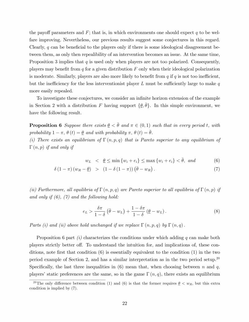
Proposition 6 Suppose there exists � < �� and � 2 (0; 1) such that in every period t, withprobability 1� �; � (t) = � and with probability �; � (t) = ��.(i) There exists an equilibrium of � (n; p; q) that is Pareto superior to any equilibrium of

� (n; p) if and only if

wL < � � min fwi + eig � max fwi + eig < ��; and (6)

� (1� �) (wR � �) > (1� � (1� �))��� � wR

�: (7)

(ii) Furthermore, all equilibria of � (n; p; q) are Pareto superior to all equilibria of � (n; p) if

and only if (6), (7) and the following hold:

eL >��

1� ���� � wL

�+1� ��1� � (� � wL) : (8)

Parts (i) and (ii) above hold unchanged if we replace � (n; p; q) by � (n; q) :

Proposition 6 part (i) characterizes the conditions under which adding q can make both

players strictly better o¤. To understand the intuition for, and implications of, these con-

ditions, note �rst that condition (6) is essentially equivalent to the condition (1) in the two

period example of Section 2, and has a similar interpretation as in the two period setup.20

Speci�cally, the last three inequalities in (6) mean that, when choosing between n and q;

players�static preferences are the same, so in the game � (n; q), there exists an equilibrium

20The only di¤erence between condition (1) and (6) is that the former requires � < wR; but this extracondition is implied by (7).

22

in which players agree to implement n in state � and q in state ��. The �rst inequality in (6)

means that p is L�s most preferred policy in either state, so status quo p is never repealed.

Hence, in the game � (n; p), if n is the status quo and R�s preference for n over p in the low

state � is stronger than her preference for p over n in the high state ��, R will not approve

intervening with p and in any equilibrium, players will stay at n forever. This is assured

by condition (7), and in that case, both players are strictly worse o¤ in this no-intervention

equilibrium path than in the equilibrium path of � (n; q), described above.

Now consider the game � (n; p; q). Since, under (7), R does not approve p, adding p

to the game leaves the incentives underlying the equilibria of � (n; q) unchanged. Agreeing

to implement n in state � and q in state ��, therefore, is also an equilibrium of � (n; p; q)

and both players strictly prefer it to the unique equilibrium path of � (n; p). Hence, for the

ine¢ cient instrument to be bene�cial in some equilibrium, players�degree of polarization

must be su¢ ciently large so that they disagree su¢ ciently often on when to repeal p; but

not so large that they agree su¢ ciently often on when to repeal q:

Part (ii) shows that the additional condition (8) is required to ensure both players are

strictly better o¤ in all equilibria of � (n; p; q) relative to � (n; p). The reason is that IE and

EE may coexist in � (n; p; q): staying with n inde�nitely, as in the unique equilibrium path

of � (n; p), may remain an equilibrium in � (n; p; q), leaving L and R indi¤erent between

the two games. To see how this can occur, suppose that L threatens to approve only p if

ever q is implemented. If such a threat is credible, R never approves q and no intervention

is ever implemented. Condition (8) guarantees that no such threat is credible: when eL is

su¢ ciently large, L prefers to accept n rather than stay at q in state �. Thus, to guarantee

that both players bene�t unambiguously from the availability of q, q must be su¢ ciently

ine¢ cient for the less interventionist players.

It is worth noting how the conditions of Proposition 6 depend on � and �. From (7) and

(8), the set of wR, wL and eL that satisfy these conditions expands as � falls. Hence, both

players are more likely to bene�t from q if the state in which they disagree over interven-

ing with the e¢ cient policy becomes more likely. And as � increases and players become

more patient, the set of wR satisfying (7) increases and a welfare improving IE equilibrium,

therefore, becomes more likely. However, the right hand side of (8) �rst decreases and then

increases with �. Hence, to bene�t unambiguously from the presence of q, players should be

su¢ ciently, but not excessively, patient.21

21The nonmonotonic impact of � on the value of ine¢ cient instument is not an artifact of the two-statedistributions considered in Proposition 6. Condition (6) guarantees that players are in full ideological agree-ment when choosing between the ine¢ cient instrument q and no intervention n. This makes q particularlyattractive. If the distribution of the state has full support, su¢ ciently patient players may introduce anine¢ cient gridlock also to the choice between n and q. As a result, unlike in the two-state case, q may not

23

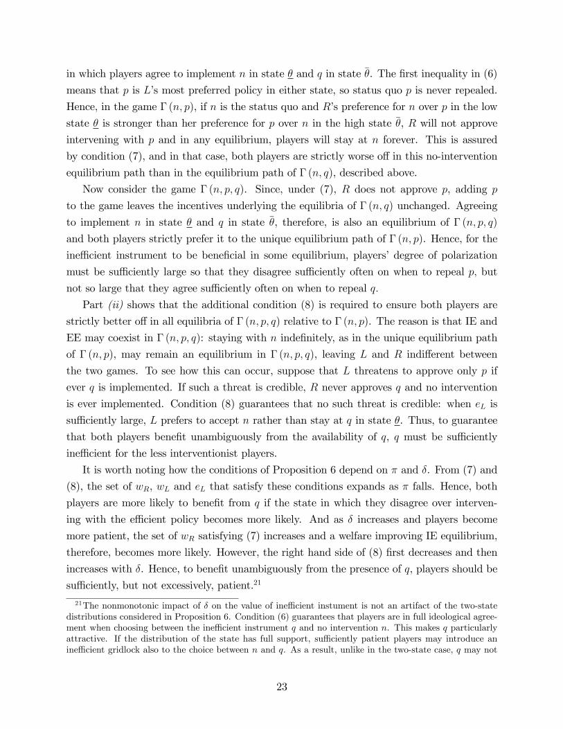
The main message of Proposition 6 remains unchanged even if we allow for non-Markov

strategies. Indeed, if conditions (6) and (7) are satis�ed, then there exists a SPNE of

� (n; p; q) that Pareto dominates any SPNE of � (n; p). To see this, simply note that under

condition (6), having policy p forever gives a strictly greater payo¤to L than any other policy

path. So in any SPNE of � (n; p), p stays in place forever once it becomes the status quo.

Thus, condition (7) implies than in any SPNE of � (n; p) ; the initial status quo n stays in

place forever. The Markov equilibrium � of � (n; p; q) in which players agree to implement n

in state � and q in state �� is a fortiori a SPNE, and from what precedes, it Pareto dominates

any SPNE of � (n; p) : Note further that under conditions (6) and (7), allowing for non-

Markov strategies does not lead to more e¢ cient outcomes. Since under (6) in any SPNE p

stays in place forever once implemented, the path of � is the most preferred path of R among

all such paths, so � is R�s most preferred SPNE. Outside of the environment of Proposition 6,

allowing for non-Markov strategies may expand the set of equilibria to include more e¢ cient

ones, but the main qualitative message of the paper should survive, namely, that q may be

used in equilibrium and ruling out q, either by selecting a di¤erent equilibrium or by allowing

players to commit not to use q, can make them worse o¤.

5 Volatility and Persistent States

Until now, states, and thereby players�state-contingent preferences, have been assumed i.i.d.

draws over time. In many applications, however, there may be periods of relative stability

when players do not expect to change their positions, other things equal, and there may

also be periods in which new information about the desirability of an intervention arrives

frequently, resulting in frequent revisions of the relevant policy preferences.22 Our main

argument, therefore, that one reason for rational legislators to reject an e¢ cient policy in

favor of an ine¢ cient policy is because ine¢ cient policies are easier to repeal, is attenuated

to the extent that it depends essentially on the i.i.d. assumption. Consequently, we extend

the argument to a more general environment in which the i.i.d. assumption is relaxed to

permit serial correlation.

To capture the possibility that states may persist across periods in an analytically

tractable way, and to allow for players�expectations regarding the persistence of the current

strictly improve both players�payo¤s if players are su¢ ciently patient and, further, an IE may not exist.22A painful example is the US Congressional response to the 2008 �scal collapse. For some years before

2008, the US economy was growing strongly and atypical Congressional economic interventions were minimal.The fall of Lehman Brothers and the subsequent turmoil in much of the global economy led to seriousCongressional disagreement regarding the appropriate level and duration of any extraordinary intervention,from whether to bail out banks or the car industry, to extensions of unemployment and welfare bene�ts.

24

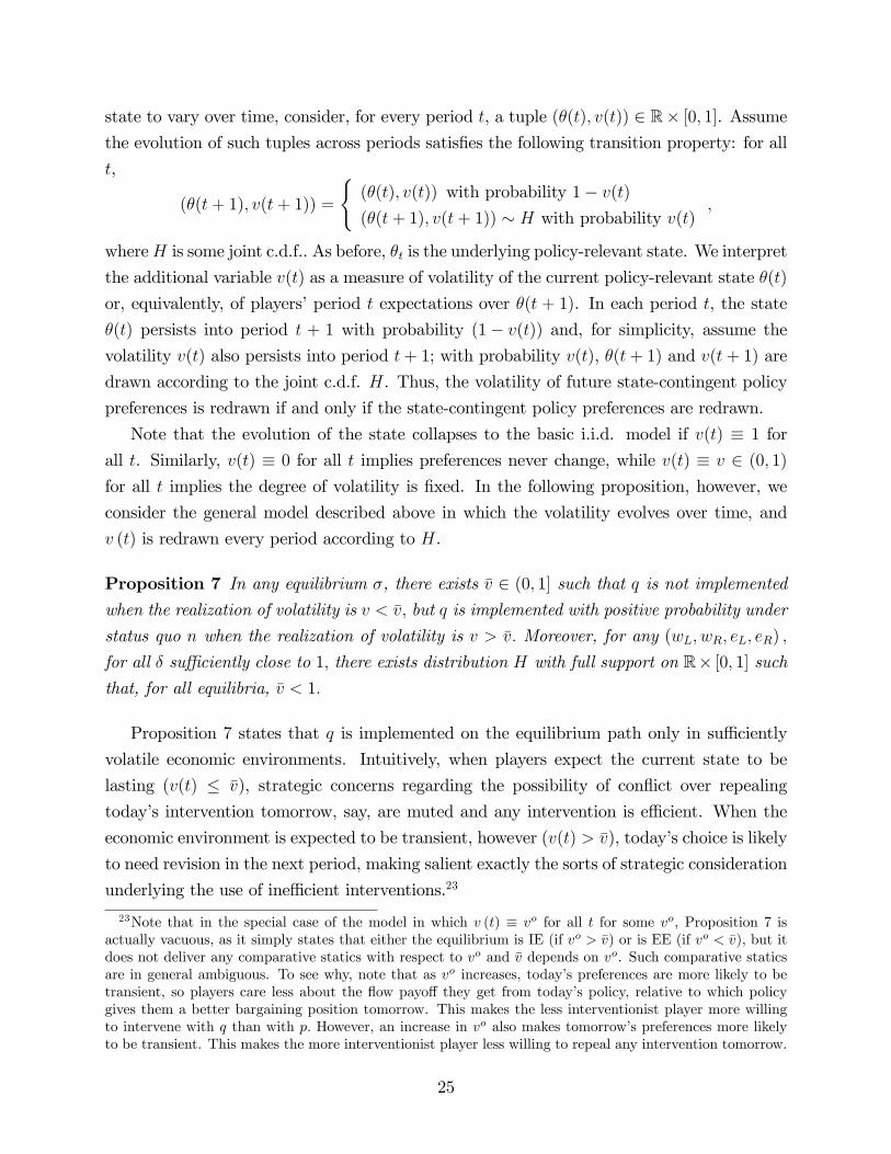
state to vary over time, consider, for every period t, a tuple (�(t); v(t)) 2 R� [0; 1]. Assumethe evolution of such tuples across periods satis�es the following transition property: for all

t,

(�(t+ 1); v(t+ 1)) =

((�(t); v(t)) with probability 1� v(t)(�(t+ 1); v(t+ 1)) � H with probability v(t)

;

whereH is some joint c.d.f.. As before, �t is the underlying policy-relevant state. We interpret

the additional variable v(t) as a measure of volatility of the current policy-relevant state �(t)

or, equivalently, of players�period t expectations over �(t + 1). In each period t, the state

�(t) persists into period t + 1 with probability (1� v(t)) and, for simplicity, assume thevolatility v(t) also persists into period t+ 1; with probability v(t), �(t+ 1) and v(t+ 1) are

drawn according to the joint c.d.f. H. Thus, the volatility of future state-contingent policy

preferences is redrawn if and only if the state-contingent policy preferences are redrawn.

Note that the evolution of the state collapses to the basic i.i.d. model if v(t) � 1 for

all t. Similarly, v(t) � 0 for all t implies preferences never change, while v(t) � v 2 (0; 1)for all t implies the degree of volatility is �xed. In the following proposition, however, we

consider the general model described above in which the volatility evolves over time, and

v (t) is redrawn every period according to H.

Proposition 7 In any equilibrium �, there exists �v 2 (0; 1] such that q is not implementedwhen the realization of volatility is v < �v; but q is implemented with positive probability under

status quo n when the realization of volatility is v > �v: Moreover, for any (wL; wR; eL; eR) ;

for all � su¢ ciently close to 1; there exists distribution H with full support on R� [0; 1] suchthat, for all equilibria, �v < 1:

Proposition 7 states that q is implemented on the equilibrium path only in su¢ ciently

volatile economic environments. Intuitively, when players expect the current state to be

lasting (v(t) � �v), strategic concerns regarding the possibility of con�ict over repealing

today�s intervention tomorrow, say, are muted and any intervention is e¢ cient. When the

economic environment is expected to be transient, however (v(t) > �v), today�s choice is likely

to need revision in the next period, making salient exactly the sorts of strategic consideration

underlying the use of ine¢ cient interventions.23

23Note that in the special case of the model in which v (t) � vo for all t for some vo, Proposition 7 isactually vacuous, as it simply states that either the equilibrium is IE (if vo > �v) or is EE (if vo < �v), but itdoes not deliver any comparative statics with respect to vo and �v depends on vo. Such comparative staticsare in general ambiguous. To see why, note that as vo increases, today�s preferences are more likely to betransient, so players care less about the �ow payo¤ they get from today�s policy, relative to which policygives them a better bargaining position tomorrow. This makes the less interventionist player more willingto intervene with q than with p: However, an increase in vo also makes tomorrow�s preferences more likelyto be transient. This makes the more interventionist player less willing to repeal any intervention tomorrow.

25

6 Conclusion

The continued and widespread use of ine¢ cient policy interventions in more-or-less demo-

cratic political systems is a puzzle. For example, while economists uniformly recommend reg-

ulating emissions with Pigou taxes, technology and quantity controls are the most adopted

instruments in reality. Why would rational politicians agree on the use of Pareto dominated

policy instruments? In our model, an ine¢ cient policy intervention may arise even when

there is no salient legislative history or vested interest. Rather, an ine¢ cient policy may

be chosen precisely because it is ine¢ cient and the environment is expected to change in

the future. From this perspective, the puzzle alluded to above can be understood without

pointing to informational asymmetries, interest group in�uence, or di¤erential distributional

implications of alternative policy instruments among the electorate at large.

With a heterogeneous legislature and multiple veto players, ine¢ cient interventions are

politically easier than e¢ cient interventions to repeal in dynamic environments subject to

policy-relevant stochastic shocks. And since ine¢ cient interventions are easier to repeal,

heterogeneous veto players, di¤erentiated only by the threshold shocks beyond which they

judge some policy intervention to be warranted, can be more willing to agree on responding

to a su¢ ciently severe downside shock with an ine¢ cient instrument. As a consequence,

ine¢ cient interventions are more likely to be used in (moderately) polarized political envi-

ronments and for issues where the fundamentals are subject to change over time.

7 References

Acemoglu, D., and J. A. Robinson, 2000. "Why Did the West Extend the Franchise," Quar-

terly Journal of Economics 115, 1167-99.

Acemoglu, D. and J. A. Robinson, 2001. "A Theory of Political Transitions", American

Economic Review 91, 938-63.

Aidt, T., 2003. "Economic Analysis of Corruption: A Survey", Economic Journal 113, 632-

52.

Alesina, A., and S. Ardagna. 2013. "The Design of Fiscal Adjustments." Tax Policy and

the Economy 27: 19-68.

Alesina, A. and A. Drazen, 1991. "Why Are Stabilizations Delayed?" American Economic

Review: 81, 1170-88.

Alesina, A., C. Favero, F. Giavazzi, O. Barbiero, and M. Paradisi, 2017. "The E¤ects of

The greater inertia under q or p has an ambiguous e¤ect on the willingness of the less interventionist playerto use q:

26

Fiscal Consolidations: Theory and Evidence", Working Paper.

Alesina, A. and F. Passarelli, 2014. "Regulation vs Taxation", Journal of Public Economics

110, 147-56.

Alesina, A., R. Perotti, and J. Tavares. 1998. "The Political Economy of Fiscal Adjust-

ments. " Brookings Papers on Economic Activity Spring: 197-266.

Ali, N., M. Mihm and L. Siga, 2017. "The Perverse Politics of Polarization", Working Paper.

Anesi, V. and J. Duggan, 2017. "Existence and Indeterminacy of Markovian Equilibria in

Dynamic Bargaining Games", forthcoming in Theoretical Economics.

Anesi, V. and D. Seidmann, 2015. "Bargaining in Standing Committees with an Endogenous

Default", Review of Economic Studies 82, 825-867.

Austin, D. and M. Levit, 2010. Mandatory Spending Since 1962. Congressional Research

Service.

Bagwell, K. and R. Staiger, 1990. "A Theory of Managed Trade", American Economic Re-

view 80, 779-795.

Baldursson, F. M. and N-H. M. von der Fehr, (2007). "A Whiter Shade of Pale: On the Po-

litical Economy of Regulatory Instruments", Journal of the European Economic Association

5(1):37�65.

Bardhan, P., 1971. "On the Optimum Subsidy to a Learning Industry: An Aspect of the

Theory of Infant-Industry Protection", International Economic Review 12, 54-70.

Baron, D. 1996. "A Dynamic Theory of Collective Goods Programs", American Economic

Review 90, 316-30.

Becker, G. and C. Mulligan, 2003. "Deadweight Costs and the Size of Government", Journal

of Law and Economics, 46, 293-340.

Bernheim, D., A. Rangel and L. Rayo, 2006. "The Power of the Last Word in Legislative

Policy Making", Econometrica 74, 1161�1190.

Blackwell, D. "Discrete Dynamic Programming." The Annals of Mathematical Statistics 33,

no. 2 (1962): 719-26.

Bowen, T., Y. Chen and H. Eraslan, 2014. "Mandatory Versus Discretionary Spending: the

Status Quo E¤ect", American Economic Review 104, 2941-2974.

Bowen, T., Y. Chen, H. Eraslan and J. Zapal, 2017. "E¢ ciency of Flexible Budgetary In-

stitutions", Journal of Economic Theory, 167, 148-176.

Brady, David W., and Craig Volden. 2006. Revolving Gridlock: Politics and Policy from

Jimmy Carter to George W. Bush. 2nd ed. Boulder, CO: Westview Press.

Buisseret, P., and D. Bernhardt. 2017. "Dynamics of Policymaking: Stepping Back to Leap

Forward, Stepping Forward to Keep Back?, American Journal of Political Science, 1-16.

Buisseret, P., and D. Bernhardt. 2018. "Reelection and Renegotiation: International Agree-

27

ments in the Shadow of the Polls?, forthcoming in American Political Science Review.

Canes-Wrone, B., M. Herron and K. Shotts, 2001. "Leadership and Pandering: A Theory

of Executive Leadership", American Journal of Political Science 45, 532-550.

Coate, S. and S. Morris, 1995. "On the Form of Transfers to Special Interests", Journal of

Political Economy 103, 1210-35.

Cox, G. and M. McCubbins, 2000. "Political Structure and Economic Policy: The Institu-

tional Determinants of Policy Outcomes", in Presidents, Parliaments and Policy, Stephan

Haggard and Mathew McCubbins (eds.), Cambridge, Cambridge University Press.

Diermeier, D. and P, Fong, 2011. "Legislative Bargaining with Reconsideration", Quarterly

Journal of Economics 126, 947�985.

Duggan, J. and T. Kalandrakis, 2012. "Dynamic Legislative Policy Making", Journal of

Economic Theory 147, 1653�1688.

Drazen, A. and N. Limao, 2008. "A Bargaining Theory of Ine¢ cient Redistribution Poli-

tics", International Economic Review 49, 621-57.

Dziuda, W. and A. Loeper, 2016. "Dynamic Collective Choice with Endogenous Status

Quo", Journal of Political Economy 124, 1148-1186.

Dziuda, W. and A. Loeper, 2018. "Dynamic Pivotal Politics", forthcoming in American

Political Science Review.

Fearon, J. D., 1998. "Commitment Problems and the Spread of Ethnic Con�ict." In The

International Spread of Ethnic Con�ict, ed. David A. Lake and Donald Rothchild. Prince-

ton, NJ: Princeton University Press.

Fernandez, R. and D. Rodrik, 1991. "Resistance to Reform: Status Quo Bias in the Presence

of Individual-Speci�c Uncertainty." American Economic Review 81, 1146-55.

Gale, W. and P. Orszag, 2003. "Sunsets in the Tax Code", Tax Notes 99, 1553-1561.

Glaeser, E. L. and G. Ponzetto, 2014. "Shrouded Costs of Government: The Political Econ-

omy of State and Local Public Pensions." Journal of Public Economics, 116, 89-105.

Grossman, G. and E. Helpman, 2001. Special Interest Politics, Cambridge MA, MIT Press.

Grossman, G. and E. Helpman, 1994. "Protection for Sale", American Economic Review

84, 833-50.

Hassler, J., J. Rodriguez Mora, K. Storesletten and F. Zillibotti, 2003. "The Survival of the

Welfare State", American Economic Review 93(1), 87-112.

Jorgenson, D., R. Goettle, M. Ho and P. Wilcoxen, 2013. Double Dividend: Environmental

Taxes and Fiscal Reform in the United States, Cambridge MA, MIT Press.

Kalandrakis, T., 2004. "A Three-Player Dynamic Majoritarian Bargaining Game", Journal

of Economic Theory 116, 294-322.

Krehbiel, K., 1998. Pivotal Politics: A Theory of U.S. Lawmaking, Chicago, University of

28

Chicago Press

Mankiw, N. G., 2010. "Crisis Economics", National A¤airs (summer): 21-32.

Masciandaro, D. and F. Passarelli, 2013. "Financial Systemic Risk: Taxation or Regula-

tion?", Journal of Banking and Finance 37, 589-96.

Melitz, M., 2005. "When and How Should Infant Industries be Protected?", Journal of In-

ternational Economics 66, 177-196.=

Mooney, C., 2004. "A Short History of Sunsets", Legal A¤airs, Jan.-Feb.

Ortner, Juan, 2017. "A Theory of Political Gridlock", Theoretical Economics 12: 555-586.

Posner, E. and A. Vermeule, 2002. "Legislative Entrenchment: A Reappraisal", Yale Law

Journal 111, 1665-1705.

Powell, R., 2004. "The Ine¢ cient Use of Power: Costly Con�ict with Complete Informa-

tion", The American Political Science Review, 98(2), 231-241.

Riboni, A. and F. Ruge-Murcia, 2008. "The Dynamic (In)e¢ ciency of Monetary Policy by

Committee", Journal of Money, Credit, and Banking: 40(5), 1001-1032.

Spolaore, E., 2004. "Adjustments in Di¤erent Government Systems", Economics and Poli-

tics 16, 117-146.

Strulovici, B., 2010. "Learning While Voting: Determinants of Collective Experimentation",

Econometrica 78(3): 933-71.

Tullock, G., 1967. Towards a Mathematics of Politics, Ann Arbor: University of Michigan

Press.

Tullock, G., 1993. Rent Seeking, London: Edward Elgar Publishing.

Villas-Boas, M., 1997. "Comparative Statics of Fixed Points", Journal of Economic Theory

73, 183�198.

Weingast, B., K. Shepsle and C. Johnson, 1981. "The Political Economy of Bene�ts and

Costs: A Neoclassical Approach to Distributive Politics", Journal of Political Economy 89,

642-664.

Zapal, J., 2011. "Explicit and Implicit Status-Quo Determination in Dynamic Bargaining:

Theory and Application to FOMC Directive", Working Paper, CERGE-EI, Prague.

8 Appendix

8.1 Notations and Preliminary Lemmas

Notation 1 Throughout the appendix, the term�strategy� refers to a Markov strategy, theterm equilibrium refers to a Markov perfect equilibrium, and we allow mixed strategies (in

the behavioral sense). That is, we assume that in each period t, each player i privately

29

observes the realization of a payo¤-irrelevant random variable �i (t) and can condition her

action in period t only on payo¤ relevant variables and on �i (t), where f�L (t) : t 2 Ng andf�R (t) : t 2 Ng are i.i.d. and independent of each other.For a given strategy pro�le �, the policy outcome in period t 2 N with status quo s (t) 2fn; p; qg can depend on the following exogenous stochastic factors: the state of nature � (t),the identity p (t) of the proposer recognized in period t, and the realization of players�pri-

vate randomization devices (�L (t) ; �R (t)). Let � (t) � (� (t) ; p (t) ; �L (t) ; �R (t)) denote therandom variable that encodes this information. We refer to � (t) as the state of the world

in period t: Let � denote the set of possible states of the world. Note that f� (t) : t 2 Ngis i.i.d.. Let � denote its probability distribution. For any state of the world � 2 �; � (�)denotes the corresponding realization of the state of nature: For all s; x 2 fn; p; qg ; �� (s; x)denotes the set of realizations of the state of the world for which status quo s leads to outcome

x if players play �:

Let V �i (�; x) denote the expected discounted payo¤ for player i 2 fL;Rg from implementing

policy x 2 fn; p; qg in period 0 conditional on �(0) = �; and on players playing � from period1 onwards.

Lemma 2 characterizes the continuation payo¤ parameters introduced in Lemma 1 (equi-

librium existence will be established latter on). Lemma 2 also derives some necessary con-

ditions on (w�; e�) for � to be an equilibrium. Lemma 3 provides necessary and su¢ cient

conditions on (w�; e�) for � to be an EE. These conditions will allow us to derive conditions

on the primitive parameters under which no EE exists, and thus under which all equilibria

are IE (see the proof of Proposition 3).

De�nition 2 Let (wc; ec) 2 R4: A strategy pro�le � is subgame perfect for the continuationpayo¤ parameters (wc; ec) 2 R4 if � is a subgame perfect equilibrium of the game in which

players play a single period of � with payo¤s V de�ned by: for all � 2 R; Vi (�; p)�Vi (�; n) =� � wci and Vi (�; p)� Vi (�; q) = eci .

Lemma 2 Let � be a strategy pro�le.

A) Recall the de�nition of V � from Notation 1. There exist w�i 2 R and e�i 2 R such that,for all � 2 R;

V �i (�; p)� V �i (�; n) = � � w�i ; (9)

V �i (�; p)� V �i (�; q) = e�i ;

V �i (�; q)� V �i (�; n) = � � w�i � e�i :

30

Expression w�i �wi�

(e�i �ei�) is equal to the expected payo¤ gain for player i of having

initial status quo n (p) instead of p (q) in the game � given continuation play �.

B) Let w�i and e�i be the continuation payo¤ parameters of �; as characterized in (9). Then

� is an equilibrium if and only if � is subgame perfect for w�i and e�i in the sense of

De�nition 2.

C) If � is an equilibrium, then

w�i � wi�

=

Z��(p;p)\��(n;n)

(w�i � � (�)) d� (�)�Z��(p;p)\��(n;q)

e�i d� (�) ; (10)

e�i � ei�

=

Z��(p;p)\��(q;q)

e�i d� (�) +

Z��(p;p)\��(q;n)

(� (�)� w�i ) d� (�) (11)

+

Z��(p;n)\��(q;q)

(w�i + e�i � � (�)) d� (�) :

Proof. By de�nition, V �i (�; p) � V �i (�; n) is the sum of the �ow payo¤ gain from im-

plementing p instead of n in t = 0 when � (0) = � and � times the continuation payo¤ gain

from period 1 onwards from having s(1) = p instead of s(1) = n; given continuation play �

in t � 1: So using Notation 1, we can write

V �i (�; p)�V �i (�; n) = ��wi+ �X

x;y2fn;p;qg

Z��(p;x)\��(n;y)

(V �i (� (�) ; x)� V �i (� (�) ; y)) d� (�) :

Therefore, to prove the �rst line of (9), it su¢ ces to set

w�i � wi � �X

x;y2fn;p;qg

Z��(n;x)\��(p;y)

(V �i (� (�) ; x)� V �i (� (�) ; y)) d� (�) : (12)

An analogous reasoning on the continuation payo¤ gain from implementing p instead of q

proves the second line of (9) with

e�i � ei + �X

x;y2fn;p;qg

Z��(p;x)\��(q;y)

(V �i (� (�) ; x)� V �i (� (�) ; y)) d� (�) : (13)

The third line of (9) is simply the sum of the �rst two.

Using De�nition 2 and Part A, Part B simply restate the fact that � is a Markov perfect

equilibrium if and only if in any period t, � prescribes actions that are subgame perfect given

continuation play � from t+ 1 onwards.

31

To prove part C, let � be an equilibrium. Using (13), we get e�i �ei�=P

x;y2fn;p;qg e�i (x; y),

where

e�i (x; y) �Z��(p;x)\��(q;y)

(V �i (� (�) ; x)� V �i (� (�) ; y)) d� (�) : (14)

For x = y clearly e�i (x; y) = 0: Consider next (x; y) = (q; n) ; that is, status quo p is

replaced by q; and status quo q is replaced by n: Since � is an equilibrium, for all � 2�� (p; q) \ �� (q; n) ; both players must weakly prefer to implement q to p and n to q inperiod 1; given continuation play �: Moreover, one of them must be indi¤erent between

implementing n and q; because if both players strictly preferred to implement n to q in

state v; then under status quo p; either veto player would accept n; so proposing n instead

of q in that period would be a pro�table deviation for the proposer. Therefore, for all

� 2 �� (p; q) \ �� (q; n) ; V �i (�(�); q) � V �i (�(�); n) = 0 for some player i; and using (9),

this implies � (�)�w�i � e�i = 0. But that equality is satis�ed only in states of the world forwhich the corresponding realization of the state of nature is � (�) = w�i + e

�i ; but since F is

continuous, this happens with probability 0, so � (�� (p; q) \�� (q; n)) = 0; and so e�i (q; n) =0: In the case (x; y) = (p; n) ; an analogous reasoning implies that � (�� (q; p) \�� (p; n)) = 0so e�i (p; n) = 0: Consider now (x; y) = (q; p) ; that is, status quo p is replaced by q and vice

versa. Since � is an equilibrium, for all � 2 �� (p; q) \�� (q; p) ; V �i (�(�); p) = V �i (�(�); q)for both players, so from (14), e�i (q; p) = 0. The only remaining cases are (x; y) equal to

(p; q), (p; n), and (n; q) ; so (13) becomes

e�i � ei�

=

Z��(p;p)\��(q;q)

(V �i (� (�) ; p)� V �i (� (�) ; q)) d� (�)

+

Z��(p;p)\��(q;n)

(V �i (� (�) ; p)� V �i (� (�) ; n)) d� (�) +Z

��(p;n)\��(q;q)

(V �i (� (�) ; n)� V �i (� (�) ; q)) d� (�) :

Substituting (9) into the above expression, we obtain (11).

The proof of (10) follows a similar logic. Using (12), we get that w�i �wi�

=P

x;y2fn;p;qgw�i (x; y),

where w�i (x; y) �R��(p;x)\��(n;y) (V

�i (� (�) ; x)� V �i (� (�) ; y)) d� (�) : Using the same steps

as the ones used to prove � (�� (p; q) \�� (q; n)) = 0 and reversing the role of p and q; weobtain that � (�� (p; n) \�� (n; q)) = 0; so w�i (n; q) = 0: An analogous reasoning implies

that � (�� (p; q) \�� (n; p)) = 0; so w�i (q; p) = 0. Moreover, for all � 2 �� (p; n)\�� (n; p) ;each player i must be indi¤erent between implementing n and p, so � (�) � w�i � e�i = 0:

Since F is continuous, this implies that � (�� (p; n) \�� (n; p)) = 0, so w�i (n; p) = 0. Theonly remaining cases left are (x; y) equal to (p; n), (p; q), and (q; n) : Equation (10) follows

then from substituting these three cases into the right-hand side of (12) and using (9).

32

Lemma 3 (Necessary and Su¢ cient Conditions for EE)

A) Let � be an EE. Then e�L > 0; e�R � 0; w�L < wL < wR < w�R; �� (q; q) � �� (p; p) ; and

for all i 2 fL;Rg ;w�i � wi�

=

Z w�R

w�L

(w�i � �) dF (�) : (15)

B) For any � that is EE, there exists �0 that is also EE and is such that players never

propose q under any status quo, w�0= w� and for all i 2 fL;Rg ;

e�0i � ei�

=

Z minnw�L+e

�0L ;w

�R

ow�L

bR (�; q) (� � w�i ) dF (�) : (16)

C) Reciprocally, if there exists (w�; e�) 2 R4 such that e�R � 0 and such that

w�i � wi�

=

Z w�R

w�L

(w�i � �) dF (�) ; and (17)

e�i � ei�

=

Z minfw�L+e�L;w�Rg

w�L

bR (�; q) (� � w�i ) dF (�) ; (18)

then there exists an EE � such that the corresponding continuation payo¤ parameters

(w�; e�) (as de�ned in Lemma 2A) satisfy (w�; e�) = (w�; e�).

Proof. Proof of part A: Let � be an arbitrary EE.Step A1: w�L < w

�R and for all i 2 fL;Rg ;

w�i � wi�

=

Z��(p;p)\��(n;n)

(w�i � � (�)) d� (�) : (19)

Since � is an EE, � (�� (n; q)) = 0: Substituting the latter equality into (10), we obtain (19).

Taking di¤erences across players in (19) and solving for w�R � w�L, we obtain w�R � w�L =wR�wL

1���(��(p;p)\��(n;n)) > 0:

Step A2: e�L � 0 and e�R � 0Note �rst that in any state � > w�k + e

�k ; from Lemma 2A, player k strictly prefers imple-

menting q to n; given continuation play �; and if e�k < 0; k also prefers implementing q to

p: So if e�i < 0 for some i 2 fL;Rg ; then since � is an equilibrium, in any period t in whichs (t) = n, i is the proposer, and � (t) > maxk2fL;Rg fw�k + e�kg ; the other player j must acceptproposal q; so i must propose q, which contradicts � being an EE.

Step A3: modulo a zero measure set, �� (p; p) = f� 2 � : � (�) > w�Lg and �� (n; n) =f� 2 � : � (�) < w�Rg :

33

From Lemma 2A, for all � 2 � such that � (�) > w�L; L strictly prefers implementing p ton given continuation play �; and since � is an equilibrium, � =2 �� (p; n) : Since � is an EE,� (�� (p; q)) = 0: By de�nition of ��; (�� (p; x))x2fn;p;qg is a partition of �; so necessarily,

� 2 �� (p; p). Conversely, for all � 2 � such that � (�) < w�L; from Step A1, � (�) < w�R;

so both players strictly prefer implementing n to p given continuation play �: Since � is

an equilibrium, necessarily, � =2 �� (p; p) : Since F is continuous, the set of � such that

� (�) = w�L has probability 0; which completes the proof of the �rst equality in Step A3.

From Lemma 2A, for all � 2 � such that � (�) < w�R; R strictly prefers implementing n

to p given continuation play �; and since � is an equilibrium, � =2 �� (n; p) : Since � is anEE, � (�� (n; q)) = 0: Since (�� (n; x))x2fn;p;qg is a partition of �; necessarily, � 2 �� (n; n).Conversely, for all � 2 � such that � (�) > w�R, from Step A1, � (�) > w�L; so from Lemma

2A, both players strictly prefer implementing p to n, given continuation play �: Therefore,

� =2 �� (n; n) : The second equality in Step A3 follows then from the continuity of F .

Step A4: (w�L; w�R) satis�es (15) and w

�L < wL < wR < w

�R.

From Step A3, modulo a zero measure set, �� (p; p)\�� (n; n) = f� 2 � : � (�) 2 (w�L; w�R)g.Substituting this equality into (19), we obtain (15). Step A1 and the assumption that F has

full support implyR w�Rw�L(w�L � �) dF (�) < 0 <

R w�Rw�L(w�R � �) dF (�) : Together with (15), the

above inequalities imply w�L < wL < wR < w�R:

Step A5: e�L > 0

Let us �rst prove that � (�� (p; n) \�� (q; q)) = 0: Suppose by contradiction that the latterprobability is positive. Then from Lemma 2A, for some � 2 �� (p; n)\�� (q; q) ; both playersstrictly prefer implementing n to p and one player weakly prefers implementing q to n; given

continuation play �: From Lemma 2A, this means that mini fw�i + e�i g � � (�) < w�L and,

therefore, mini fw�i + e�i g < w�L; a contradiction with Step A1 and A2.Substituting � (�� (p; n) \�� (q; q)) = 0 into (11), we get

e�i � ei�

=

Z��(p;p)\��(q;q)

e�i d� (�) +

Z��(p;p)\��(q;n)

(� (�)� w�i ) d� (�) : (20)

From Step A3, for almost all � 2 �� (p; p) ; � (�) > w�L; so (20) implies e�L � eL > 0:Step A6: �� (q; q) � �� (p; p)

Let � 2 �� (q; q) : Since � is an equilibrium, in state �; one player weakly prefers implement-ing q to n given continuation play �; so � (�) � min fw�L + e�L; w�R + e�Rg : From Steps A1,

A2, and A5, the latter inequality implies � (�) > w�L: From Step A3, � 2 �� (p; p).Proof of part B: Recall that an EE is an equilibrium in which q is never implemented

on path given initial status quo n: This de�nition does not prevent players to propose and

34

implement q under status quo q; and this may happen in an EE � such that e�k = 0 for some

k: For such EE, formula (15) is more complicated. So in this part, we prove that for any

EE �; there always exists an EE �0 such that w�0= w� and q is never implemented even

under status quo q: We construct �0 as the limit of a sequence��k�k2N de�ned recursively

from � as follows. We set �0 = �: For any k � 0; we de�ne �k+1 as a function of �k as

follows. Consider �rst the action nodes of veto player i 2 fL;Rg : When comparing n andp; i plays �. When comparing p and q; i votes for p. When comparing n and q; i votes for

q when � (�) > w�i + e�k

i and for n otherwise. Consider now the action nodes of proposer

i 2 fL;Rg : When the status quo is n or p; i plays �. When the status quo is q; L proposesn when � � w�L; and p otherwise, and R proposes n when � � min

nw�L + e

�k

L ; w�R

oand p

otherwise.

Step B1: for all k 2 N, w�k = w�and e�1L � e�0LBy construction, for all k 2 N; �k prescribes the same actions as � when neither the statusquo nor the proposal is q; and these actions never lead to outcome q: So the value of the game

� with initial status quo n (p) is the same with continuation play �k and �: From Lemma

2A, this implies w�k= w�: When the status quo is q, by construction of �1; �1 always

implements n or p; and �1 prescribes actions that are subgame perfect given continuation

play �: So the actions prescribed by � and �1 under status quo q may di¤er only in an

action node in which one player is indi¤erent between two actions. Lemma 2A implies that

a given player can be indi¤erent between implementing n and p (n and q) only in a unique

state. Since F is continuous, this means that she can be indi¤erent between two actions in a

nonnegligibe set of states only when one action leads to outcome p whereas the other leads

to outcome q (and when e�R = 0). In those cases, �1 always prescribes R to choose p; which

is what L prefers given continuation play � since from part A of this Lemma, e�L > 0: So

under status quo q; L is weakly better o¤ when �1 is played than when � is played in the

current period, given continuation play �: Since the continuation path of �1 and � coincide

under status quo n or p, this implies that under status quo q; L weakly prefers continuation

play �1 to continuation play �. From Lemma 2A, this means that e�1

L � e�0L :Step B2: for all k 2 N, e�kL > 0 and

e�k+1

i � ei�

=

Z minnw�L+e

�k

L ;w�R

ow�L

bR (�; q) (� � w�i ) dF (�) : (21)

We prove Step B2 by induction. Since �0 = � is an EE, Part A of this lemma implies e�0

L > 0.

Suppose now e�k

L > 0 for some k 2 N, and let us show (21) and e�k+1L > 0. From Lemma

2A,�e�

k+1

L � ei�=� is the expected payo¤ gain from having status quo p instead of q given

35

continuation play �k+1. To compute it, note that from Part A of this lemma, w�L < w�R; and

since e�k

L > 0, we have w�L < minnw�L + e

�k

L ; w�R

o: So by construction of �k+1, on path, status

quo q and p both lead to outcome n when � < w�L; and they both lead to outcome p when

� > w�R; when � 2 (w�L; w�R) and L is the proposer, and when � 2�min

nw�L + e

�k

L ; w�R

o; w�R

�and R is the proposer. Modulo a negligible set of states, the only remaining cases is when R

is the proposer and � 2�w�L;min

nw�L + e

�k

L ; w�R

o�: In those cases, status quo q and p lead

to outcome n and p, respectively, so from Lemma 2A, the relative continuation payo¤ gain

is � � w�k+1i = � � w�i : Integrating over all these cases, we obtain (21). From Part A of this

lemma, w�L < w�R; so (21) implies e

�k+1

L > eL > 0:

Step B3: for all k � 1; e�k+1L � e�kL and e�k+1

R � e�kR .We prove Step B3 by induction. From Steps B1 and B2, e�

1

L � e�0L : Suppose now e�k+1

L � e�kLfor some k 2 N. From Step B2,

e�k+2

i � e�k+1i = �

Z minnw�L+e

�k+1

L ;w�R

ominfw�L+e�kL ;w�Rg

bR (�; q) (� � w�i ) dF (�) :

Since e�k

L � e�k�1L ; R.H.S. of the above is negative for i = L and positive for i = R:

Step B4: �k+1 prescribes subgame perfect actions given continuation play �k.

From Part A of this lemma, e�0

R � 0: Steps B2 and B3 imply then that for all i 2 fL;Rg andk 2 N; e�ki � 0. So using Lemma 2A, one can check check that by construction of

��k�k2N,

�k+1 prescribes the veto player to approve (reject) the proposal when she strictly prefers the

proposal (status quo) given continuation play �k; and that �k+1 prescribes the proposer to

propose the policy that she prefers among those accepted by the veto player.

Step B5: �0 � limk!1 � exists and satis�es the properties stated in Part B.

From Steps B1 and B3, w�k

i and e�k

i have a limit as k !1, and since �k+1 is a cuto¤strategyin which the cuto¤s are continuous functions of w�

k

i and e�k

i , it has a limit �0. From Step

B4, by continuity, �0 is an equilibrium, and by construction of��k�k2N ; �

0 never prescribes

proposal q, so � is an EE. Taking the limit in (21), we obtain (16).

Proof of part C: Suppose (w�; e�) 2 R4 solves (17) and (18) with e�R � 0: Construct

a strategy pro�le � as follows. Consider �rst the action nodes of veto player i 2 fL;Rg :When comparing n and p; i votes for p when � > w�i and for n otherwise. When comparing

p and q; i votes for p. When comparing n and q; i votes for q when � (�) > w�i + e�i and for

n otherwise. Consider now the action nodes of proposer i 2 fL;Rg : When the status quois n or p; i proposes p when � > w�i and n otherwise, When the status quo is q; L proposes

n when � � w�L; and p otherwise, and R proposes n when � � min fw�L + e�L; w�Rg and potherwise. By construction, q is never implemented on path. Therefore, to complete the

36

proof, it su¢ ces to show that � is an equilibrium. From Lemma 2B, it su¢ ces to show that

� is subgame perfect given continuation payo¤ parameters (w�; e�) ; and that (w�; e�) (as

de�ned in Lemma 2A) coincides with (w�; e�). This is what Steps C1 to C3 below do.

Step C1: � is subgame perfect for the continuation payo¤ parameters (w�; e�) in the

sense of de�nition 2.

By assumption, e�R � 0, and since e� satis�es (18), we have e�L � eL > 0; so both players

always weakly prefer to implement p to q: So one can easily check that by construction of �, �

prescribe either veto players to accept (reject) a proposal when it gives her a greater (lesser)

continuation payo¤, given continuation payo¤ parameters (w�; e�). Likewise, � prescribe

either proposer to propose the policy that gives her the greatest continuation payo¤ among

those accepted by the veto player, given continuation payo¤ parameters (w�; e�).

Step C2: w� = w�:

Since w� satis�es (17), the same reasoning as in Step A1 implies w�L < w�R: By con-

struction of �; q is never implemented on path, and status quo n and p lead to di¤erent

outcomes only when � 2 (w�L; w�R) ; in which case either status quo stay in place, and

the corresponding continuation payo¤ gain is w�i � �. From Lemma 2A, this means thatw�i �wi�

=R w�Rw�L(w�i � �) dF (�) : This equation can be viewed as a linear equation in w�i ; and

it has a unique solution. From (17), w�i is also a solution to that equation, so w�i = w

�i .

Step C3: e� = e�:

The same reasoning as in Step B2 (taking w� = w� and e�k

L = e�L) shows that by construction

of �; modulo a negligible set of states, status quo p and q lead to di¤erent outcomes only

when R is the proposer and � 2 (w�L;min fw�L + e�L; w�Rg) ; in which case status quo p andq lead to outcome p and n, respectively, and the corresponding continuation payo¤ gain is

� � w�i : Therefore, Lemma 2A implies thate�i �ei�

=R minfw�L+e�L;w�Rgw�L

bR (�; q) (� � w�i ) dF (�) :Together with (18), that equation implies e�i = e

�i .

8.2 Proofs for Section 4

Proof of Lemma 1. The second claim of Lemma 1 follows from Lemma 2A. The rest of

the proof establishes the �rst claim, i.e., equilibrium existence. For all i 2 fL;Rg ; let �i bea correspondence de�ned on R such that for all eci 2 R;

�i (eci) �

8><>:[0; 1] if eci = 0

0 if eci < 0

1 if eci > 0

: (22)

De�ne the correspondence � � (�L;�R) :

37

The structure of the proof is as follows. In Step 1, for any continuation payo¤parameters

(wc; ec) 2 R4, we construct a set of strategy pro�les that are subgame perfect for the con-tinuation payo¤ parameters (wc; ec) in the sense of De�nition 2. In particular, for any given

(wc; ec) ; player i has strict preferences between n and p and between n and q for almost all

realizations of �; and we assume then that when indi¤erent, player i takes action that results

in the implementation of n: Hence, we uniquely determine the subgame-perfect behavior of

player i when choosing between n and any intervention. When choosing between p and q;

we allow each player to randomize, and we use �i to denote the probability that i chooses to

implement q: Hence, for any (wc; ec) and any mixing rule � 2 [0; 1]2 ; we construct a uniquestrategy pro�le. Let � (�;wc; ec) denote this strategy pro�le and let w�(�;w

c;ec) and e�(�;wc;ec)

be the unique continuation payo¤ parameters associated with this strategy pro�le as de�ned

in Lemma 2. rom (22), whenever � 2 �(ec) ; � (�;wc; ec) is subgame-perfect for the contin-uation payo¤ parameters (wc; ec). We de�ne the correspondence � that maps R4 � [0; 1]2

into itself as follows:24

� (wc; ec; �) ���w�(�;w

c;ec); e�(�;wc;ec); �0

�: �0 2 �

�e�(�;w

c;ec)�: (23)

Note that the strategies used to de�ne � are subgame perfect only for � 2 �(ec) and

not for all � 2 [0; 1]2 ; but by construction of �, if (��; w�; e�) is a �xed point of �; �� 2�(e�) and � (��; w�; e�) is subgame perfect for the continuation payo¤ parameters (w�; e�) =�w�(�

�;w�;e�); e�(��;w�;e�)

�: From Lemma 2B, this means that � (��; w�; e�) is an equilibrium.

Thus, to prove equilibrium existence, it su¢ ces to show that � has a �xed point. The rest

of the proof then checks that � satis�es the conditions of Kakutani�s �xed point theorem.

Step 2 shows that there exists a compact and convex set C such that � (C) � C, Steps 3

and 4 show that the graph of � is closed, and Step 5 shows that � is convex-valued.

Step 1: For each (�;wc; ec), we construct a strategy pro�le � (�;wc; ec) that is subgame

perfect for the continuation payo¤ parameters (wc; ec) (in the sense of De�nition 2) when-

ever players choose between n and p or n and q; but uses � as the tie-breaking rule between

p and q. Whenever � 2 �(ec) ; this strategy pro�le is subgame perfect.The construction of � (�;wc; ec) is intuitive, but the detailed description below will be use-

ful in Step 3 to show that the continuation payo¤ parameters derived from � (�;wc; ec) are

24Note that � is not a mapping from strategy space to strategy space as is usual in �x-point-type existenceproofs. The reason for this is that the set of strategies that are subgame perfect for the continuationparameters (wc; ec) may be quite complex whenever ec = 0; and showing convexity or contractibility of suchset may be an issue. Instead, we take as a primitive (wc; ec) together with a tie-breaking rule, and map itinto the payo¤ parameters generated by a strategy that uses this tie-breaking rule and is subgame perfectwith respect to (wc; ec) and into a set of new tie-breaking rule that are subgame perfect with respect toe�(�;w

c;ec):

38

continuous in (�;wc; ec). In this description, for brevity, players�preferences should be un-

derstood as their preferences given continuation payo¤ parameters (wc; ec).

Veto-player�s strategy: In any Markov state in which the veto player i 2 fL;Rg hasthe choice between n and p (n and q); �i prescribes i to choose n when she weakly prefers

implementing n, i.e., when � � wci (when � � wci + eci), and �i prescribes i to choose p (q)otherwise.

When the veto player has to choose between p and q; �i prescribes i to choose p with proba-

bility (henceforth w.p.) �i and q w.p. 1� �i; irrespective of �. From (22), when � 2 �(ec) ;this behavior is subgame perfect given continuation payo¤ parameters (wc; ec).

Finally, when the status quo is proposed, the action prescribed by �i is irrelevant.

Proposer�s strategy under status quo p: When i weakly prefers p to n or when �jprescribes j to veto proposal n (i.e., when � � wci or � > wcj), then �i prescribes proposer ito propose p w.p. �i and q w.p. 1��i (note that by what precedes, the veto player strategyis independent of the proposer�s strategy). When � 2 �(ec) ; this is subgame perfect giventhe veto-player�s strategy �j and continuation payo¤ parameters (wc; ec), because in both

cases, i always weakly prefers proposing the status quo p to proposing n; and from (22),

when � 2 �(ec) ; �i prescribes i to propose q only when she weakly prefers it to p.The remaining case is when i strictly prefers n to p and �j prescribes j to accept proposal

n (i.e., when �i < wc and �j � wc). In this case, from Lemma 2A, the continuation payo¤

gain for i from proposing n instead of p is wci � �, whereas that of proposing q instead of p is��jeci . So when wci � � > ��jeci ; proposal n dominates both proposals q and p; and we set�i to prescribe i to propose n:When wci �� � ��jeci ; proposal n is dominated by proposal q.So �i prescribes i to propose p w.p. �i and q w.p. 1� �i. From (22), when � 2 �(ec) ; thisis subgame perfect under status quo p given the veto player�s strategy �j and continuation

payo¤ parameters (wc; ec).

Proposer�s strategy under status quo q: analogous to the proposer�s strategy understatus quo p; where the role of p and q and their corresponding continuation payo¤ parame-

ters are reversed.

Proposer�s strategy under status quo n: When i weakly prefers n to p and n to q (i.e.,when � � min fwci ; wci + ecig), �i prescribes i to propose n; which is optimal since n is thestatus quo.

When i strictly prefers p to n and weakly prefers n to q (i.e., when wci < � � wci + eci), �

prescribes i to propose p; which is optimal for i irrespective of whether j accepts it.

When i strictly prefers q to n and weakly prefers n to p (i.e., when wci + eci < � � wci ), �

prescribes i to propose q; which is optimal for i irrespective of whether j accepts it.

The only remaining case is when i strictly prefers q and p to n (i.e., when � > maxi2fL;Rg fwci ; wci + ecig).

39

In that case, if �j prescribes j to veto both p and q (i.e., � � min�wcj ; w

cj + e

cj

), �i prescribes

i to propose n: If �j prescribes j to veto q but not p (i.e., wcj < � � wcj + ecj), �i prescribes ito propose p: If �j prescribes j to veto p but not q (i.e., wcj + e

cj < � � wcj), �i prescribes i to

propose q. Finally, if both p and q are accepted (i.e., � > min�wcj ; w

cj + e

cj

), �i prescribes i

to propose p w.p. �i and q w.p. 1� �i.Step 2: There exists a compact and convex set C such that � (C) � C:

Let B � maxifjwij+jeij+E(j�j)g1�� and C � [�B;B]4� [0; 1]2 : The compactness and convexity of C

is obvious. To see why � (C) � C, note that from (4), the �ow payo¤di¤erence between anytwo policies is bounded by E [j�j+ jwij+ jeij] ; so the expected discounted payo¤ di¤erencebetween any two policy paths is bounded by B � E[j�j]+jwij+jeij

1�� : Therefore, by de�nition of

w�i and e�i (see Lemma 2A), for any strategy pro�le �; jw�i j+ je�i j is bounded by B:

Step 3: The functions (�;wc; ec)! w�(�;wc;ec) and (�;wc; ec)! e�(�;w

c;ec) are continuous.

By construction of � (see Step 1), for all � 2 R; x; y 2 fn; p; qg, (�;wc; ec) 2 C; the probabilitythat in state �; � (�;wc; ec) prescribes the proposer to propose y (the veto player to accept

y) under status quo x is piece-wise constant in �: Moreover, on each of the intervals on

which it is constant in �; this probability is continuous in (�;wc; ec), and the bounds of these

intervals depend continuously on (�;wc; ec). Therefore, the probability that on the path of

� (�;wc; ec), status quo x is replaced by policy y in some state � is continuous in (�;wc; ec)

except at a �nite number of �. Using Notation 1, the continuity of F implies then that the

expectation of V �(�;wc;ec)

i (�; x) conditional on � � F is continuous in (�;wc; ec). From (12)

and (13), this implies that w�(�;wc;ec)

i and e�(�;wc;ec)

i are continuous in (�;wc; ec) :

Step 4: � has a closed graph.

Let��k; wk; ek

�k2N and

��k; wk; ek

�k2N be two sequences inC that converge to some (�

1; w1; e1)

and (�1; w1; e1)k2N, respectively, and such that for all k 2 N,��k; wk; ek

�2 �

��k; wk; ek

�:

We need to show that (�1; w1; e1) 2 � (�1; w1; e1) : From (23) and (22),��k; wk; ek

�2

���k; wk; ek

�implies that wk = w�(�

k;wk;ek), ek = e�(�k;wk;ek); and �k 2 �

�ek�: From Step

3, w1 = w�(�1;w1;e1) and e1 = e�(�

1;w1;e1): So it remains to establish that �1 2 �(e1) ;which requires that e1 > 0 implies �1 = 1; and e1 < 0 implies �1 = 0: Note that e1 > 0

implies ek > 0 and thus �k = 1 for k large enough, so e1 = 1: A similar argument establishes

the second implication.

Step 5: � is convex-valued.

One can immediately check from (22) that �(:) is convex-valued, so from (23), � is also

convex-valued.

Proof of Proposition 2. Let � be an arbitrary IE, and let i; j 2 fL;Rg be such thatw�i � w�j in this equilibrium.Step 1: � (�� (p; p) \�� (q; n)) > 0.

40

Since � is an equilibrium, in any state � 2 �� (p; n) , each player k must prefer implementingn to p given continuation play �; so Lemma 2A implies � (�) � w�k ; and therefore, w

�k +

e�k � � (�) � e�k . Substituting the latter inequality in the equilibrium formula for e�k ; (11), weobtain

e�k � ek�

�Z(��(p;p)[��(p;n))\��(q;q)

e�kd� (�) +

Z��(p;p)\��(q;n)

(� (�)� w�k ) d� (�)

) e�k �ek + �

R��(p;p)\��(q;n) (� (�)� w

�k ) d� (�)

1� �� ((�� (p; p) [�� (p; n)) \�� (q; q)) : (24)

Suppose by contradiction that � (�� (p; p) \�� (q; n)) = 0: Then (24) implies e�L > 0 and

e�R > 0; so both players always strictly prefer to implement p to q given continuation play

�: Since � is an equilibrium, this implies that q is never implemented on path, which is

impossible since � is an IE.

Step 2: mink2fL;Rgw�k < mink2fL;Rg (w�k + e

�k) :

Since � is an equilibrium, for all � 2 �� (q; n) ; both players weakly prefer implementing nto q given continuation play �; so from Lemma 2A, � (�) � w�k + e

�k for both k 2 fL;Rg.

For all � 2 �� (p; p) ; at least one player weakly prefers implementing p to n; i.e., � (�) � w�kfor some k 2 fL;Rg. So for all � 2 � (�� (p; p) \�� (q; n)) ; mink2fL;Rgw�k � � (�) �mink2fL;Rg (w

�k + e

�k) : Since from step 1, �� (p; p) \ �� (q; n) has positive probability, and

since F is continuous, the latter weak inequalities must be strict for some � 2 �� (p; p) \�� (q; n) ; which implies Step 2.

Step 3: e�j � 0 and e�i > ei > 0:Since � is an equilibrium, for all � 2 �� (p; p) ; some player weakly prefers implementing p ton; so � (�) � mink2fL;Rgw�k = w�i : Since F is continuous, this inequality is strict for almostall � 2 �� (p; p) : Substituting � (�) > w�i and Step 1 into (24), we get e

�i > ei > 0. As

argued in Step 1, since � is an IE, e�i > 0 implies e�j � 0:

Step 4: w�i < w�j :

From Step 3, e�j � 0; so (24) impliesR�2��(p;p)\��(q;n)

�� (�)� w�j

�d� (�) < 0. Therefore,

there exists �o � �� (p; p) \ �� (q; n) such that � (�o) > 0 and for all �o 2 �o, � (�o) <w�j : From Lemma 2A, the latter inequality implies that for all �o 2 �o; j strictly prefersimplementing n to p given continuation play �. Since �o � �� (p; p) and � is an equilibrium,i must weakly prefer implementing p to n in such states �o, i.e., � (�o) � w�i : The latter

inequality, together with � (�o) < w�j ; implies w�i < w

�j :

Proof of Proposition 3 Parts (i) and (ii) and Part (iii) in the case wR�wL ! 0.An equilibrium is either an EE or an IE, so all equilibria are IE if and only if no EE

exist. Lemma 3 implies that no EE exist if and only if there exists no (w�; e�) 2 R2 such that

41

e�R � 0 and (17) and (18) hold. The proof proceeds by deriving conditions on the primitiveparameters such that any solution (w�; e�) to (17) and (18) must be such that e�R < 0.

Step 0: Notations.

Condition (17) depends on (w; e) only through w; so let W � (w) denote the set of w� 2 R2

solving (17) for i = L;R. If we �x w� and eL, condition (18) for i = L can viewed as a

�xed point in e�L: It depends on (w; e) only through w� and eL; so let E�L (w

�; eL) denote the

set of e�L solving (18) for i = L. Since the R.H.S. of (18) is continuous and bounded in e�L;

E�L (w�; eL) is nonempty and closed, so let e�L (w

�; eL) denote its minimum. Finally, if we �x

w�, e�L, and eR; (18) for i = R pins down a unique e�R which we denote e

�R (w

�; e�L; eR) :

Step 1: for all w� 2 W � (w), e�L (w�; eL) is weakly increasing in eL; and e�R (w

�; e�L; eR) is

weakly increasing in eR and weakly decreasing in e�L:

Since the R.H.S. of (18) for i = L is continuous in (eL; e�L) and weakly increasing in eL;

Theorem 1 in Villas Boas 1997 implies that the smallest �xed point e�L (w�; eL) is weakly

increasing in eL: The comparative statics on e�R (:) follow readily from (18) for i = R and the

fact that for all w� 2 W � (w) ; w�L < w�R (see Lemma 3A).

Step 2: no EE exists if and only if for all w� 2 W (w), e�R�w�; e�L (w

�; eL) ; eR

�< 0.

As explained at the beginning of this proof, no EE exists if and only if for all solutions to

(17) and (18), e�R < 0. Using the notations of Step 0 and the comparative statics established

in Step 1, no EE exists if and only if e�R�w�; e�L (w

�; eL) ; eR

�< 0 for all w� 2 W � (w).

Step 3: Proof of Proposition 3 Parts (i) and (ii).

Part (ii) follows from Step 2, together with the comparative statics on eL established in Step

1. Likewise, Step 2, together with the comparative statics on eR established in Step 1 proves

Part (i) for some �eR 2 [0;+1_]. To complete the proof of Part (ii) ; it su¢ ces to show that0 < �eR < +1:To show that �eR < +1, observe �rst that for any w� and e�L the R.H.S. of (18) for i = Ris bounded below by �E[j�j]� w�i which is independent of e�L and eR: So for any w�; for eRsu¢ ciently large, e�R

�w�; e�L (w

�; eL) ; eR

�> 0; so an EE exists, as needed.

Let us now show that �eR > 0. Let w� 2 W � (w) : As shown in Step A1 in the proof of Lemma

3, w�L < w�R; so (18) for i = L implies that e�L (w�; eL) � eL > 0: Finally, (18) for i = R

implies

limeR!0

e�R

�w�; e�L (w

�; eL) ; eR

�= �

Z minfw�L+e�L(w�;eL);w�Rg

w�L

bR (�; q) (� � w�R) dF (�) :

Since F has full support and bR (�; q) > b > 0 for all � 2 R; the R.H.S. of the above equationis strictly negative. Step 2 implies then that for eR su¢ ciently small, no EE exists.

42

Step 4: Proof of Proposition 3 Part (iii) in the case wR � wL ! 0.

Suppose Proposition 3 Part (iii) is false in the case wR � wL ! 0. Then from step 2,

there exists�wk�k2N such that w

kR � wkL ! 0 and for all k 2 N; for all w�;k 2 W � �wk�,

e�R

�w�;k; e�L

�w�;k; eL

�; eR

�< 0: Taking di¤erences across players in (17), we obtain w�;kR �

w�;kL =wkR�wkL

1��(F(w�;kR )�F(w�;kL ))

� wkR�wkL1�� ; so w�;kR > w�;kL and w�;kR � w�;kL !k!1 0. Since w�;kR >

w�;kL , (18) for i = R implies e�R

�w�;k; e�L

�w�;k; eL

�; eR

�� eR+�

R w�;kRw�;kL

bR (�; q)�� � w�;kR

�dF (�) :

Since w�;kR � w�;kL !k!1 0; continuity of F implies that the R.H.S of the above inequality

tends to eR > 0 as k !1, which contradicts that e�R�w�;k; e�L

�w�;k; eL

�; eR

�< 0.

The next lemma will be used to prove Proposition 3 Part (iii).

Lemma 4 If � is an equilibrium, then

e�i = ei + �

Z��(q;q)

e�i d� (�) +

Z��(p;p)\��(q;n)

(� (�)� w�i ) d� (�) ; (25)

w�i = wi + �

Z��(p;p)\��(n;n)

(w�i � � (�)) d� (�)� �Z��(n;q)

e�i d� (�) : (26)

and for some D such that (1� �)2 � D � 1;

w�R � w�L =(1���(��(q;q)))[wR�wL]���(��(n;q))[eR�eL]

D;

e�R � e�L =(1���(��(p;p)\��(n;n)))[eR�eL]���(��(p;p)\��(q;n))[wR�wL]

D;

w�R + e�R � w�L � e�L =

(1���(��(p;p)\��(q;fn;qg)))[wR�wL]+(1���(��(p;p)\f��(n;n)[��(n;q)g))[eR�eL]D

:

(27)

Proof. Step 1: for any equilibrium �; �� (q; q) � �� (p; p) ; �� (n; q) � �� (p; p) ; and

(26), and (25) hold.

That �� (q; q) � �� (p; p) in EE follows from Lemma 3A. Suppose now that � is an IE.

In any � 2 �� (q; q) ; some player weakly prefer implementing q to n, so from Lemma

2A, � (�) � mink2fL;Rg fw�k + e�kg : Using part (iii) of Proposition 2, the last inequalityimplies that � (�) > mink2fL;Rgw�k ; so one player must strictly prefer implementing p to n;

and therefore � =2 �� (p; n) : From part (ii) of Proposition 2, e�i > 0 so from Lemma 2A,

� =2 �� (p; q) : Since (�� (p; x))x2fn;p;qg is a partition of �; this implies � 2 �� (p; p) ; as

needed.

To show �� (n; q) � �� (p; p) ; let � 2 �� (n; q) : Since � is an equilibrium, in state

� (�) both players must weakly prefer implementing q to n, so from Lemma 3A, � (�) �maxi2fL;Rg fw�i + e�i g : Using Lemma 3A (for an EE) and part (iii) of Proposition 2 (for anIE), we have

maxi2fL;Rg

fw�i + e�i g � mini2fL;Rg

fw�i + e�i g > mini2fL;Rg

fw�i g ;

43

so � (�) > mini2fL;Rg fw�i g ; which means that one player strictly prefers implementing p ton; and therefore � =2 �� (p; n) : Since �� (p; q) = ;; and since (�� (p; x))x2fn;p;qg is a partitionof �; necessarily, � 2 �� (p; p) ; as needed.Substituting �� (n; q) � �� (p; p) into (10), we obtain (26). Finally, by de�nition of ��,

�� (p; n)\�� (p; p) = ;; so �� (q; q) � �� (p; p) implies �� (p; n)\�� (q; q) = ;: Substitutingthe latter equality and �� (q; q) � �� (p; p) into (11), we obtain (25).Step 2: Proof of the �rst two lines of (27).

Subtracting (26) for i = R from (26) for i = L; and doing the same for (25), we get(w�R � w�L = wR � wL + �� (�� (p; p) \�� (n; n)) (w�R � w�L)� �� (�� (n; q)) (e�R � e�L)e�R � e�L = eR � eL + �� (�� (q; q)) (e�R � e�L)� �� (�� (p; p) \�� (q; n)) (w�R � w�L)

:

The above equations can be viewed as a linear system in w�R�w�L and e�L�e�R: Straightforwardalgebra shows that its solution is given by the �rst two lines of (27) for

D � (1� �� (�� (p; p) \�� (n; n))) (1� �� (�� (q; q)))��2� (�� (p; p) \�� (q; n))� (�� (n; q)) :

Step 3: Proof of the third line of (27).

From Step 1, �� (q; q) � �� (p; p) and, by de�nition of��; �� (q; n) and�� (q; q) are disjoint,so

� (�� (p; p) \�� (q; n)) + � (�� (q; q)) = � (�� (p; p) \ f�� (q; n) [�� (q; q)g) : (28)

From Step 1, �� (n; q) � �� (p; p) and, by de�nition of ��; �� (n; n) and �� (n; q) are

disjoint, so

� (�� (p; p) \�� (n; n)) + � (�� (n; q)) = � (�� (p; p) \ f�� (n; n) [�� (n; q)g) : (29)

Adding up the �rst two lines of (27) and substituting (28) and (29) into the corresponding

expression for w�R + e�R � w�L � e�L, we obtain the third line of (27) for the above D.

Step 4: (1� �)2 � D � 1:That D � 1 is obvious from the de�nition of D: To prove D � (1� �)2 ; observe that�� (q; q) and �� (p; p) \ �� (q; n) are disjoint. So �� (q; q) is included into the complementof �� (p; p)\�� (q; n) : Likewise, �� (p; p)\�� (n; n) and �� (n; q) are disjoint, so �� (p; p)\

44

�� (n; n) is included in the complement of �� (n; q) : Therefore,

D = (1� �� (�� (p; p) \�� (n; n))) (1� �� (�� (q; q)))��2� (�� (p; p) \�� (q; n))� (�� (n; q))

� (1� � (1� � (�� (n; q)))) (1� � (1� � (�� (p; p) \�� (q; n))))��2� (�� (p; p) \�� (q; n))� (�� (n; q))

= (1� �) (1� � + � (� (�� (n; q)) + � (�� (p; p) \�� (q; n)))) � (1� �)2 :

Proof of Proposition 3 Part (iii) case wR � wL ! +1.Suppose by contradiction that Part (iii) is false in the case wR�wL ! +1. Then there

exists e 2 (0;+1)2, m 2 R and two sequences�wk�k2N and (� (k))k2N with the following

properties: wkR�wkL ! +1, for all k 2 N; wkL+wkR = m; and � (k) is an IE for the �ow payo¤parameters

�e; wk

�. Below, we show that for k su¢ ciently large, e�(k)L > 0 and e�(k)R > 0;

which, from Lemma 3, contradicts the assumption that � (k) is an IE.

Step 1: for k su¢ ciently large; w�(k)L < w�(k)L + e

�(k)L < w

�(k)R + e

�(k)R � w�(k)R :

Since wkR � wkL ! +1; Equation (27) and inequality D � (1� �)2 in Lemma 4 imply that,for k large enough,

w�(k)R � w�(k)L � (1� �)

�wkR � wkL

�� jeR � eLj :

Hence, w�(k)R � w�(k)L ! +1 so for k large enough, w�(k)R > w�(k)L , and parts (i) and (ii) of

Proposition 2 imply that e�(k)L > 0 � e�(k)R : Moreover, (27) and inequality D � (1� �)2 in

Lemma 4 imply

w�(k)R + e

�(k)R � w�(k)L � e�(k)L � (1� �)

�wkR � wkL

�� jeR � eLj :

So w�(k)R + e�(k)R � w�(k)L � e�(k)L ! +1: Together with e�(k)L > 0 � e�(k)R , this implies Step 1.

Step 2: for k su¢ ciently large; e�(k)R � eR+�����(k) (q; q)

�e�(k)R +�

R w�(k)L +e�(k)L

w�(k)L

�w�(k)L � w�(k)R

�dF (�) :

Let � 2 ��(k) (p; p)\��(k) (q; n) : Since � (k) is an equilibrium, in state �; both players mustweakly prefer implementing n to q and one player must prefer implementing p to n: From

Lemma 2A, this means that mini2fL;Rgw�(k)i � � (�) � mini2fL;Rg

�w�(k)i + e

�(k)i

�: Together

with Step 1, this implies

��(k) (p; p) \��(k) (q; n) �n� 2 � : w�(k)L � � (�) � w�(k)L + e

�(k)L

o: (30)

45

From (30), for all � 2 ��(k) (p; p) \ ��(k) (q; n) ; � (�) � w�(k)L � e�(k)L : Substituting this

inequality into (25), we obtain

e�(k)L � eL + ��

���(k) (q; q)

�e�(k)L + ��

���(k) (p; p) \��(k) (q; n)

�e�(k)L ;

and therefore that e�(k)L � eL= (1� �). Since e�(k)L > 0; the latter inequality implies that e�(k)L

is bounded. From Step 1 and (30), for all � 2 ��(k) (p; p) \��(k) (q; n) ; 0 � � (�)� w�(k)R �w�(k)L � w�(k)R : The preceding inequality and (30) imply that

Z��(p;p)\��(q;n)

(� (�)� w�R) d� (�) �Z w

�(k)L +e

�(k)L

w�(k)L

�w�(k)L � w�(k)R

�dF (�) :

Substituting the above inequality into (25), we obtain Step 2.

Step 3: as k ! +1; w�(k)L ! �1, w�(k)R ! +1 and w�(k)R ����w�(k)L

��� :As shown in Step 1, wkR � wkL ! +1. Therefore, to prove Step 3, it su¢ ces to show thatw�(k)L + w

�(k)R is bounded as k ! 1. To do so, note that if we sum (25) and (26) across

players and collect the terms in factor of w�(k)L + w�(k)R and e�(k)L + e

�(k)R , we obtain

1� �����(k) (p; p) \��(k) (n; n)

������(k) (n; q)

������(k) (p; p) \��(k) (q; n)

�1� ��

���(k) (q; q)

� ! w�(k)L + w

�(k)R

e�(k)L + e

�(k)R

!

=

m� �

R��(k)(p;p)\��(k)(n;n) � (�) d� (�)

eL + eR +R��(k)(p;p)\��(k)(q;n) � (�) d� (�)

!:

Using the notations and results in Lemma 4, the determinant of that system is D; which

is bounded away from 0 as k ! 1. Moreover, all the coe¢ cients of the above system are

bounded. Therefore, the solution w�(k)L + w�(k)R must be bounded as k !1; as needed.

Step 4: for k su¢ ciently large; e�(k)L > 0 and e�(k)R > 0.

Step 1 establishes that for k large enough, e�(k)L > 0. Let us now prove that e�(k)R > 0. Step

3 together with the integrability of F implies thatR w�(k)L +e

�(k)L

w�(k)L

w�(k)L dF (�)! 0. Substituting

this limit in Step 2, we obtain e�(k)R > 0; as needed.

Proof of Proposition 4. The strategy of the proof follows the intuition provided in

the main text after Proposition 4. We show that one can pick��; ���and [m; �m] such that if

the aforementioned sequence of EE (� (k))k2N exists, then w1L < m < min fw1L + e1L ; w1R g :

The latter inequalities mean that as k !1; with probability arbitrarily close to 1; the stateis such that players agree to repeal q (because m < min fw1L + e1L ; w1R + e1R g) but R prefersto repeal p whereas L prefers to leave it in place (because w1L < m < w1R ). Given such

expectations, for k su¢ ciently large, e�(k)R < 0: That is, R prefers to intervene with q than

46

with p; a contradiction with the assumption that � (k) is an EE.

Step 1: There exists �; ��;m; �m such that 0 < � < �� < 1 and

wL < m < �m < wL +min

��1� ��

�eL; wR � wL �

(1� �) eR�b

�< wR:

25 (31)

Since wR�wL > 0; for � su¢ ciently close to 1; minn�1� ��

�eL; wR � wL � (1��)eR

�b

o> 0; so

by continuity, we can �nd � < �� < 1 for which the interval�wL; wL +min

n�1� ��

�eL; wR � wL � (1��)eR

�b

o�is nonempty, and hence we can �nd m; �m such that the �rst three inequalities in (31) are

satis�ed. To prove the last inequality, note that wL+minn�1� ��

�eL; wR � wL � (1��)eR

�b

o�

wR � (1��)eR�b

< wR:

Step 2: Let �1 � limk!1R minnw�(k)L +e

�(k)L ;w

�(k)R

ow�(k)L

bR (�; q) dFmk;dk (�) � 0. Then

w1i = wi +�

1� � (wi �m) ; (32)

e1i = ei ���1

1� � (wi �m) : (33)

Since we suppose that � (k) are EE for all k 2 N; from Lemma 3A, we have for all k 2 N;

w�(k)i = wi + �k

Z w�(k)R

w�(k)L

�w�(k)i � �

�dFmk;dk (�) ; (34)

and w�(k)L < wL < wR < w�(k)R . As dk ! 0; the support of Fk becomes increasingly concen-

trated around m; and from Step 1, wL < m � m � �m < wR. So if we let k !1 in (34), we

obtain w1i = wi+� (w1i �m) ; which implies (32). From Lemma 3B, we can assume w.l.o.g.

that � (k) satis�es (16), so

e�(k)i = ei + �k

Z minnw�(k)L +e

�(k)L ;w

�(k)R

ow�(k)L

bR (�; q)h(� �m) +

�m� w�(k)i

�idFmk;dk (�) : (35)

If we let k ! 1 in (35) and use the de�nition of �1, we obtain e1i = ei + ��1 (m� w1i ) :

Substituting (32) into the latter equation, we obtain (33).

Step 3: e1R < 0:

Summing (32) and (33) for i = L, we obtain

w1L + e1L = wL + eL +

� (1� �1)1� � (wL �m) : (36)

47

From Step 1, m � m > wL; so the R.H.S. of (36) is increasing in �1 and since �1 � 0; (36)implies

w1L + e1L �

wL + (1� �) eL � �m1� � : (37)

From Step 1, m < wL+(1� �) eL: Substituting this inequality into the R.H.S of (37), we ob-tain w1L +e

1L > m: Since w

1L < m < w1R ; this implies that w

1L < m < min fw1L + e1L ; w1R g :

Using the latter inequalities in the de�nition of �1, we obtain �1 � b: From Step 1,

m < wR � (1��)eR�b

; so wR � m > (1��)eR�b

: Substituting the latter inequality into (33), we

obtain e1R < eR�1� �1

b

�< 0; where the latter inequality follows from �1 � b:

The proofs of Proposition 5 relies on the proof of Proposition 6, so we provide the latter

before the former.

Proof of Proposition 6. Parts A and B below prove part (i), and parts C and D

prove part (ii).

Part A: If (6) and (7) hold, there exists an equilibrium of � (n; p; q) and of� (n; q) that is Pareto superior to any equilibrium of � (n; p).Assume (6) and (7) hold and de�ne the strategy pro�le �� (n; p; q) of � (n; p; q) as follows:

Under status quo n or q; in state � (��), both players propose and accept n (q), veto q (n),

and in both states, R vetoes p and L accepts p: Under status quo p; L proposes p and

accepts only p, whereas R proposes p and accept any proposal. The path of �� (n; p; q) is as

follows: under status quo n or q; n is implemented in state � and q in state ��, and once p is

implemented, p stays in place forever.

Below, we characterize the equilibria of � (n; p) (Step A1), show that both players strictly

prefer �� (n; p; q) to any equilibrium of � (n; p) (Step A2), and show that �� (n; p; q) is an

equilibrium of � (n; p; q) (Steps A3 to A6). We then show that there exists an equilibrium

�� (n; q) of � (n; q) that has the same path as �� (n; p; q) ; and thus that also Pareto dominates

any equilibrium of � (n; p) (Step A7).

Step A1: In any equilibrium of � (n; p), the initial status quo n stays in place forever.

Let � be an equilibrium of � (n; p). From (6), wL < �; so L gets a strictly greater �ow

payo¤ from p than from any other policy in either state. Therefore, on the path of �; once

implemented, p stays in place forever. Simple algebra shows that (7) means that in state ��

(and thus in state � as well), R strictly prefers implementing n forever to implementing p

forever. Therefore, in either state, given continuation play �; R strictly prefers implementing

n forever to p forever. Therefore, the path of � stays at the initial status quo n forever.

Step A2: Both players strictly prefer �� (n; p; q) to any equilibrium of � (n; p) :

The path of �� (n; p; q) implements n and q in state � and ��, respectively. From (6), both

players get a strictly greater payo¤ from q than from n in state ��, so they strictly prefer the

48

path of �� (n; p; q) to staying at n forever. Step A2 follows then from Step A1.

Step A3: Given continuation play �� (n; p; q) ; in either state, L strictly prefers imple-

menting p to either n or q.

On the path of �� (n; p; q) ; p stays in place forever once implemented, and from (6), p gives

a strictly greater �ow payo¤ to L than any other policy in any state.

Step A4: Given continuation play �� (n; p; q) ; both players prefer implementing n to q

( q to n) in state � ( ��).

From (6), both players get a weakly greater �ow payo¤ from n than from q (from q than

from n) in state � (��), and the same continuation value as under �� (n; p; q) ; status quo n or

q lead to the same outcome.

Step A5: Given continuation play �� (n; p; q) ; in any state, R strictly prefers implement-

ing n or q to p.

From Steps A1 and A2, R prefers implementing n and playing �� (n; p; q) thereafter to im-

plementing n forever. Moreover, (7) means that in either state, R strictly prefers n forever

to p forever, which is what happens if p is implemented and �� (n; p; q) is played thereafter.

Therefore, given continuation play �� (n; p; q), in either state, R strictly prefers implementing

n to implementing p: From Step A4, in state ��; R strictly prefers implementing q to n; so

from what precedes, she must strictly prefer implementing q to p in state ��: Since the �ow

payo¤ di¤erence between q and p is independent of �; R also strictly prefers implementing q

to p in state �:

Step A6: �� (n; p; q) is an equilibrium of � (n; p; q), and it is Pareto superior to any

equilibrium of � (n; p).

Given the preferences characterized in Steps A3-A5, the behavior prescribed by �� (n; p; q)

is sequentially rational, both players strictly prefer its path to the unique equilibrium path

of � (n; p) :

Step A7: there exists an equilibrium of � (n; q) that is Pareto superior to any equilibrium

of � (n; p).

By construction, under status quo n or q; �� (n; p; q) never prescribes player to make proposal

p: So �� (n; p; q) de�nes also an equilibrium of � (n; q) ; and A7 follows from A2.

Part B: if there exists an equilibrium of � (n; p; q) or � (n; q) that is Paretosuperior to any equilibrium �� (n; p) of � (n; p), then (6) and (7) must hold.Let � (n; p; q) be an equilibrium of � (n; p; q) that is Pareto superior to any equilibrium

of � (n; p) (argument for the case of � (n; q) is analogous and is omitted for brevity).

Step B1: wL < �.

Suppose �rst that wL � � and wR � ��. In that case, player R gets a weakly greater �ow

payo¤ from n than from p in either state, so there exists an equilibrium of � (n; p) in which R

49

unilaterally decides to stay forever at the initial status quo n. This equilibrium implements

the most preferred policy path of R, and thus cannot be dominated by any equilibrium of

� (n; p; q) ; a contradiction. Suppose now that wL � � and wR < ��. In that case, both

players get a greater �ow payo¤ from p (n) than from n (p) in state �� (�), so there exists

an equilibrium of � (n; p) in which players agree to implement n in state � and p in state��. This equilibrium path is optimal for both players and can thus not be dominated by any

equilibrium of � (n; p; q) ; a contradiction.

Step B2: wR > �.

Suppose wR � �. Then both players get a weakly greater �ow payo¤ from p than from n in

either state of nature. So there exists an equilibrium of � (n; p) in which both players�most

preferred alternative p is implemented forever, so this equilibrium cannot be dominated by

any equilibrium of � (n; p; q) ; a contradiction.

Step B3: Given continuation play � (n; p; q) ; L strictly prefers implementing p to n and

p to q; so under status quo p; p stays in place forever.

Step B3 follows from the observation that since wL < �; L gets a strictly greater �ow payo¤

from p than from any other policy in either state of nature.

Step B4: Given continuation play � (n; p; q) ; R weakly prefers implementing q to p in

either state, and R strictly prefers implementing n to q and n to p in state �:

Observe �rst that q must be implemented on the path of � (n; p; q), otherwise � (n; p) would

admit an equilibrium with the same path as � (n; p; q) ; so those equilibria would be payo¤

equivalent. From Step B3, L must veto q under status quo p; so q must be implemented

with positive probability in some state �� 2��; ��under status quo n: Since from Step B3,

L strictly prefers implementing p to q; R must weakly prefer implementing q to p in state

��. Since the �ow payo¤ di¤erence between p and q and the distribution of future states is

independent of the current state, this must be the case in either state, which proves the �rst

claim of Step B4. Since q gives a strictly lower �ow payo¤ than p to R, the �rst claim of

Step B4 implies that R strictly prefers status quo q to status quo p. So it must be that in

some state �0, with positive probability, status quo q leads to some outcome x that R strictly

prefers to p and q: So x must be n: From the �rst claim of Step B4, this implies R strictly

prefers implementing n to p in state �0. Since the �ow payo¤ gain from n relative to p or q

is decreasing in �, this is true for �0 = �:

Step B5: Given continuation play � (n; p; q) ; R strictly prefers implementing n to p in

any state, so under status quo n; p is never implemented.

Suppose Step B5 is false. Since from Step B4, R strictly prefers n to p in �; it must be that

R weakly prefers implementing p to n in state ��. Using Step B3, this means that in state��, R weakly prefers implementing p forever to n forever, since R can unilaterally impose the

50

latter policy path under status quo n: Since R gets a greater �ow payo¤ from n than from p

in state �, and since L gets a strictly greater �ow payo¤ from p than from n in either state,

this implies that there exists an equilibrium of � (n; p) in which the initial status quo n stays

in place as long as the state stays at �; and p is implemented at the �rst occurrence of ��

and stays in place forever after. This equilibrium implements L�s most preferred policy path

from the �rst occurrence of state �� onwards. By assumption, L is strictly better o¤ under

� (n; p; q). For that to be the case, it must be that at the initial status quo n and in state �;

� (n; p; q) implements q or p with positive probability, a contradiction with Step B4.

Step B6: Under status quo n or q; p is never implemented on the path of � (n; p; q).

Suppose Step B6 is false. From Step B5, this implies that p is implemented with positive

probability under status quo q: From Step B4, this means that given continuation play

� (n; p; q), R is indi¤erent between implementing q or p in any state. So from Steps B5, R

strictly prefers implementing n to p and to q in any state, so R must weakly prefer staying

at n forever to playing � (n; p; q). Since she can unilaterally impose n forever in � (n; p) ; she

must weakly prefer any equilibrium of � (n; p) to � (n; p; q) ; a contradiction.

Step B7: Given continuation play � (n; p; q) ; both players strictly prefer implementing q

to n in state ��.

Suppose Step B7 is false. Given the �ow payo¤ speci�cation, this means that some player

weakly prefers implementing n to q in either state. From Step B6, this implies that she

must weakly prefer staying at n forever to playing � (n; p; q). Since she can unilaterally

impose n forever in � (n; p) ; she must weakly prefer any equilibrium of � (n; p) to � (n; p; q) ;

a contradiction.

Step B8: With probability 1; status quo n stays in place in � and is replaced by q in ��.

That n stays in place in state � follows immediately from Step B4. That it is replaced by q

with probability 1 follows from Steps B5 and B7.

Step B9: Status quo q stays in place with probability 1 in state ��; in state �, it is replaced

with positive probability by n and stays in place with the remaining probability.

That q stays in place with probability 1 in state �� follows from Steps B5 and B7. Suppose

now that status quo q is never replaced by n in state �: From Step B6, this implies that q

must stay in place with probability 1: But then both players strictly prefer implementing p

forever, so � (n; p; q) is not an equilibrium, a contradiction.

Step B10: Condition (6) must be satis�ed.

The �rst inequality of (6) comes from Step B1. For the path of play described by Steps

B8 and B9 to be an equilibrium, both players must get a weakly greater (smaller) �ow

payo¤ from n than from q in state � (��). This means that the last three inequalities in (6)

must hold weakly. Suppose by contradiction that the last inequality holds with equality.

51

Then one player must be indi¤erent between staying at n forever and the equilibrium path.

Since she can unilaterally impose n forever in the game � (n; p) ; she must weakly prefer any

equilibrium of � (n; p) to � (n; p; q) ; a contradiction.

Step B11: Condition (7) must be satis�ed.

Consider the strategy pro�le � (n; p) of � (n; p) de�ned as follows: L always proposes p and

accepts only p, and R proposes n (p) and accepts only n (p) in state � (��). The path of play

of � (n; p) is such that n stays in place until the �rst occurrence of state ��; at which time n

is replaced by p and p stays in place forever. Since the path of play of � (n; p) implements n

until the �rst occurrence of state �� and never implements p, L must strictly prefers � (n; p) to

� (n; p; q) ; so by assumption, � (n; p) cannot be an equilibrium of � (n; p). From Step B1, R

gets a strictly greater �ow payo¤ from p than from n in either state, so the actions prescribed

by � (n; p) to L are subgame perfect given continuation play � (n; p). The actions prescribed

by � (n; p) to R under status quo p are also subgame perfect since R is not pivotal under

that status quo. From Step B2, R gets a greater �ow payo¤ from n than from p in state �,

so in that state, it is subgame perfect for R not to propose p and to veto p under status quo

n: The only remaining case is when the status quo is n and the state is ��. Since � (n; p) is

not an equilibrium, it must be that R�s actions in that case are not subgame perfect. This

means that in state ��, R must strictly prefer staying at n forever than switching to p forever.

Simple algebra shows that this condition is equivalent to (7).

Part C: If all equilibria of � (n; p; q) are Pareto superior to any equilibrium of� (n; p), then (6), (7), and (8) must hold.Suppose all equilibria of � (n; p; q) are Pareto superior to any equilibrium of � (n; p). We

already know from Part B that (6) and (7) must be satis�ed. So to prove Part C, it su¢ ces

to prove (8). To do so, consider the following strategy pro�le �0 (n; p; q). Under status quo

p; both players propose p; L accepts only p, and R vetoes only q. Under status quo n;

both players proposes n; R accepts only n; and L vetoes only q. Under status quo q; both

players proposes p, L accepts only p; whereas R accepts any policy. By construction, the

path of play of �0 (n; p; q) implements n forever. Since either player can unilaterally impose

that outcome in the game � (n; p) ; �0 (n; p; q) is not Pareto superior to any equilibrium of

� (n; p) ; so by assumption, it cannot be an equilibrium. In what follows, we assume that (8)

is violated, we characterize players�incentives given continuation play �0 (n; p; q) (Step C1)

and show that �0 (n; p; q) is an equilibrium (Step C2), a contradiction.

Step C1: If condition (8) is violated, then given continuation play �0 (n; p; q) ; in either

state, R prefers implementing n to p to q; whereas L prefers implementing p to q to n.

Note �rst that since status quo q and p both lead to policy p, and since p gives both players

a greater �ow payo¤ than q; both players prefer implementing p to q in any state. Moreover,

52

(7) implies that in either state, R prefers implementing n forever to p forever, which is

what happens if n and p are implemented, respectively, given continuation play �0 (n; p; q).

Therefore, R prefers implementing n to p to q: To complete the proof, it remains to show

that L prefers implementing q to n in either state, given continuation play �0 (n; p; q), or

equivalently, that L prefers implementing q today and p forever after to implementing n

forever. Simple algebra shows that this is equivalent to (8) being violated.

Step C2: If condition (8) is violated, �0 (n; p; q) is an equilibrium.

It is straightforward to check that given the preferences characterized in Step C1, �0 (n; p; q)

prescribe either veto players to accept (reject) a proposal whenever it gives her a greater

(lesser) continuation payo¤, and it prescribe either proposer to propose the policy that gives

her the greatest continuation payo¤ among those accepted by the veto player, as needed.

Part D: If (6), (7), and (8) hold, any equilibrium of � (n; p; q) or � (n; q) isstrictly Pareto superior to any equilibrium of � (n; p) :Assume (6), (7), and (8). From Part A, the strategy pro�le �� (n; p; q) de�ned in Part A is an

equilibrium that it is strictly Pareto better than any equilibrium of � (n; p). So it su¢ ces to

show that any equilibrium of � (n; p; q) and � (n; q) must have the same path as �� (n; p; q).

In Steps D1 to D6 below, � is an arbitrary equilibrium of � (n; p; q) :

Step D1: Given continuation play �; in either state, status quo p always stays in place,

and L strictly prefers implementing p to n or q.

From (6), p gives a strictly greater �ow payo¤ to L than any other policy in any state. So R

strictly prefers staying forever at p to any other policy path, and she can unilaterally impose

that continuation path once p is the status quo.

Step D2: Given continuation play �; in either state, R strictly prefers implementing n

to p.

Once n is the status quo, R can unilaterally impose to stay at n forever. Since � is an

equilibrium, this implies that R must weakly prefer implementing n today and playing �

thereafter to implementing n forever. Moreover, from (7), in any state, R strictly prefers

implementing n forever to p forever, which, from Step D1, is what happens if p is implemented

and � is played thereafter. Step D2 follows then by transitivity.

Step D3: p is never implemented on the path of �.

From Step D1, p is never implemented under status quo n. So if Step D3 is false, it must be

that (i) in some state �0; p is implemented with positive probability under status quo q; and

that (ii) in some state �00; q is implemented with positive probability under the initial status

quo n: Note that (i) implies that given continuation play �; in state �0, R weakly prefers

implementing p to implementing q: Since the �ow payo¤of q relative to p is independent of �;

this must also be true in state �00: Likewise, (ii) implies that R weakly prefers implementing

53

q to n in state �00: By transitivity, R weakly prefers implementing p to n in state �00, a

contradiction with Step D2.

Step D4: Given continuation play �; in state �, both players strictly prefer implementing

n to q, so in state �, status quo n or q lead to n:

Suppose by contradiction that given continuation play �; some player i prefers implementing

q to n in state �. Since the �ow payo¤ of n relative to q is decreasing in �; i prefers

implementing q to n in both states, so from Step D3, i weakly prefers implementing q forever

to implementing n forever. But (7) means that in any state, R strictly prefers implementing

n forever to p forever, and thus to q forever. So i must be L: Simple algebra shows that

(8) implies that in state �, L prefers implementing n forever to implementing q today and p

forever after, so L must prefer n forever to q forever, a contradiction. The second claim in

Step D4 follows from the �rst claim and Step D3.

Step D5: Given continuation play �; in state ��, both players strictly prefer implementing

q to n, so in state ��, status quo n or q lead to policy q:

From Step D4, in state �; status quo n and q lead to the same outcome. Moreover, in state ��;

from (6), both players get a strictly greater �ow payo¤ from q than from n: Therefore, given

continuation play �; both players strictly prefer implementing q to n: The second claim in

Step D5 follows from the �rst claim and Step D3.

Step D6: � has the same path as �� (n; p; q) :

This Step follows directly from Steps D3, D4, and D5.

Step D7: any equilibrium of � (n; q) has the same path as �� (n; p; q) :

This step follows directly from the proof of Steps D4 and D5.

Proof of Proposition 5. Let F�;��;� denote the two-state c.d.f. of Proposition 6. In the

proof below, we �rst show that for any w; e, there exists �; �; ��; � such that the conditions (6),

(7), and (8) in Proposition 6 are satis�ed (Step 1). Under those conditions, Proposition 6 Part

(iii) implies that for the c.d.f. F�;��;�, in any equilibrium, both players strictly bene�t from

the availability of q: We then add a small, full support perturbation to the c.d.f. F�;��;� so as

to guarantee that � (t) has full support, as assumed in Proposition 5 (Step 2). By continuity,

a converging sequence of equilibria for the perturbed c.d.f. must tend to an equilibrium of

the unperturbed game (Steps 3 and 4), so when the perturbation is su¢ ciently small, in any

equilibrium, players still unanimously bene�t from the availability of q (Step 5).

Step 1: For any (w; e) ; there exists �; �� 2 R; � > 0; and a closed interval � � (0; 1) ofpositive length such that for all � 2 �, (6), (7), and (8) hold.Pick � and �� so that (6) holds. Simple algebra shows that (7), and (8) can be rewritten

as � < wR�(1��)������(����)

and � < (1��)eL+wL���(����)

: So (7) and (8) are satis�ed for some � 2 (0; 1)whenever the R.H.S. of the latter two inequalities are strictly positive. Simple algebra shows

54

that this is the case if and only if

�� � wR�� � �

< � <eL + wL � �

eL: (38)

Note that���wR���wL

< 1 and independent of �, and the R.H.S. of (38) is 1 for � = wL. So for any ��

satisfying (6) , by continuity one can pick � satisfying (6) such that any� �����wR���� ;

eL+wL��eL

�is nonempty.

Step 2: De�nitions.

Let f� (t) : t � 0g denote the i.i.d. process with the two-state c.d.f. F�;��;� of Proposition 6,for some � 2 [0; 1] and some � < ��. Let f" (t) : t � 0g be an i.i.d. process some c.d.f. Gwith full support. For any d > 0; the i.i.d. process f� (t) + d" (t) : t � 0g can be viewed asa full support perturbation of f� (t) : t � 0g. For all X � fn; p; qg, let � (d;X) be the game� in which the set of available policies is X and the payo¤ state is f� (t) + d" (t) : t � 0g ;and let � (d;X) be an arbitrary Markov strategy pro�le of � (d;X). In any proposer (veto

player) action node, the distribution over actions that � (d;X) prescribes is a function of

the current status quo (and proposal), � (t) and " (t) : So � (d;X) de�nes a strategy pro�le

of the unperturbed game � (0; X) in which in any proposer (veto player) action node, the

distribution of players�actions depend on the current status quo (and proposal), � (t), which

are payo¤ relevant in � (0; X), and on " (t) ; which is payo¤-irrelevant in � (0; X) but is

independent of the history. So " (t) can be viewed as a correlation device, and � (d;X) as

a correlated Markov strategy pro�le of � (0; X) : In what follows, we denote this correlated

strategy pro�le of � (0; X) by �0 (� (d;X)).

Step 3: Fix w; e; �; ��; � and some X � fn; p; qg. Let (dk)k2N 2 (0;+1)N and (�k)k2N 2

(0; 1)N be such that dk ! 0 and �k ! � for some � 2 (0; 1) : Using the notations of Step 2,for all k 2 N, let � (dk; X) be an equilibrium of � (dk; X) for the discount factor �k. Then

there exists a subsequence of (�0 (� (dk; X)))k2N that converges to a correlated (in the sense

of Step 2) equilibrium of � (0; X) for the limit discount factor �.

Fix k 2 N, the payo¤ parameters w; e; �k; and the parameters �; ��; � of the c.d.f. F�;��;�.As argued in Step 2, for all k 2 N; �0 (� (dk; X)) can be viewed as a (possibly correlated)Markov strategy pro�le of � (0; X) : Since � (t) can take only two values, � (0; X) has �nitely

many Markov states, and in each state, players must choose between �nitely many actions.

Therefore, there exists a subsequence of (�0 (� (dk; X)))k2N that converges to a (possibly

correlated) strategy pro�le � (0; X) of � (0; X). For any realization of " (t), � + dk" (t) and�� + dk" (t) converge to � and ��; respectively, as k ! 1: So the period payo¤s of � (dk; X)converge to the period payo¤s of � (0; X) ; and by continuity, � (0; X) must be a correlated

equilibrium of � (0; X) for the limit discount factor �:

55

Step 4: Suppose w; e; �; �; ��; � are such that conditions (6), (7), and (8) are satis�ed.

Then the path of any correlated equilibrium (in the sense of Step 2) of � (0; X) coincides

with the unique equilibrium path characterized in Step A1 for X = fn; pg (in which n staysforever) and Step D for X = fn; qg or X = fn; p; qg (in which n is implemented in � and qis implemented in ��) of the proof of Proposition 6.

To prove Step 4, the reader can easily check that the arguments in Step A1 and Step D of the

proof of Proposition 6 hold unchanged even if we allow players to use correlated strategies

(in the sense of Step 2).

Step 5 (Proof of Proposition 5): For any w; e, there exists �; �� 2 R, � 2 (0; 1) and someclosed interval � � (0; 1) such that for d su¢ ciently small, for all � 2 �; both players strictlyprefer any equilibrium of � (d; fn; p; qg) or � (d; fn; qg) to any equilibrium of � (d; fn; pg) :To see why Step 5 implies Proposition 5, note that if Step 5 is true, then for any w; e; for

the corresponding parameters �; ��; �; d;� that satisfy Step 5, the statement of Proposition

5 holds for any � 2 � if we take F equal to the c.d.f. of � (t) + d" (t).

To prove Step 5, suppose it is false for some w; e. Then for any �; �� 2 R, � 2 (0; 1), and anyclosed interval � � (0; 1) ; there exists sequences dk ! 0 and �k ! � 2 �; some X equal to

fn; qg or fn; p; qg, and a corresponding sequences of equilibria � (dk; fn; pg) of � (dk; fn; pg)and � (dk; X) of � (dk; X) such that for all k 2 N; some player weakly prefers � (dk; fn; pg)to � (dk; X). From Step 1, we can pick �; ��; �;� such that (6), (7), and (8) hold. From

Step 3, we can assume that �0 (� (dk; fn; pg)) and �0 (� (dk; X)) converge to a correlatedequilibrium � (0; fn; pg) of � (0; fn; pg) and � (0; X) of � (0; X) ; respectively. Since (6),

(7), and (8) hold, Step 4 implies that the paths of � (0; fn; pg) and � (0; X) are the unique(uncorrelated) equilibrium paths of � (0; fn; pg) and � (0; X) ; respectively, as characterizedin Step A1 and Step D of the proof of Proposition 6. Since some player i weakly prefers

� (dk; fn; pg) to � (dk; X) for all k; by continuity, i weakly prefers the equilibrium path of

� (0; fn; pg) to the equilibrium path of � (0; X). This contradicts Proposition 6 Part (ii).

8.3 Proofs for the Model of Section 5

Lemma 5 Consider the model of Section 5. For every strategy pro�le �; let V �i denote thecontinuation payo¤ for player i 2 fL;Rg of implementing policy x 2 fn; p; qg in some periodt with state (�(t); v(t)) = (�; v) 2 R� [0; 1] until the next period in which the state is redrawn,given continuation play �. There exist (wL; wR; eL; eR) 2 R4 such that, for any equilibriumstrategy pro�le � and for all i 2 fL;Rg, � 2 R, and v 2 [0; 1] ;

(1� � (1� v)) [V �i (�; v; p)� V �i (�; v; n)] = � � (1� v)wi � vw�i ;(1� � (1� v)) [V �i (�; v; p)� V �i (�; v; q)] = (1� v) ei + ve�i .

(39)

56

Proof. We use Notation 1 with the exception that a state of the world � 2 � now

also includes the realization of the volatility v: For any strategy pro�le �, all � 2 � and

s 2 fn; p; qg, let X� (�; s) denote the policy outcome in a period in which the state of the

world is �, the status quo is s; and players play �: By de�nition of V �i ;

V �i (�; v; p)� V �i (�; v; n)

= � � wi + �(

(1� v) [V � (�; v; p)� V � (�; v; n)] +vR�2� [V

� (�; v;X� (�; p))� V � (�; v;X� (�; n))] d� (v)

)

=� � (1� v)wi � v

�wi � �

R�2� [V

� (�; v;X� (�; p))� V � (�; v;X� (�; n))] d� (v)

1� � (1� v) :

If we set w�i equal to the term inside the curly brackets on the numerator of the above

fraction, then w�i depends neither � nor on v; which proves the �rst line of (39). The proof

for the second line of (39) follows an analogous argument and is omitted for brevity.

Proof of Proposition 7. Let � be an equilibrium. For q to be implemented on

some equilibrium path, some player i must weakly prefer implementing q to p in some state

(v; �) given continuation play �: From Lemma 5, we have V �i (�; v; q) � V �i (�; v; p) in somestate (v; �) 2 [0; 1)� R if and only if e�i < 0 and v > ei

ei�e�i: So if e�L � 0 and e�R � 0, for all

(v; �) 2 [0; 1)�R; V �i (�; v; p) > V �i (�; v; q) ; and the �rst part of Proposition 7 holds triviallyfor �v = 1: Suppose now that e�i < 0 for some i and let �v � ei

ei�e�i< 1: Then from Lemma 5,

for all v < �v and all � 2 R; both players weakly prefer implementing p to q in state (v; �) soq is not implemented on path in such states. When v > �v and when � is su¢ ciently large, i�s

most preferred policy given continuation play � is q; and j prefers to accept q under status

quo n; so q is implemented, as needed.

Consider a sequence of c.d.f. (Hk)k2N such that for all k 2 N; Hk (v; �) = Gk (v)F (�) ;where Gk has full support and tends to the degenerate distribution which puts probability

1 on v = 1 as k ! 1: Suppose the second claim of Proposition 7 is false. Then from what

precedes, for all k 2 N; there exists an equilibrium � (k) such that e�(k)L � 0 and e�(k)R � 0:Together with (39), the latter inequalities imply that for all � 2 R and k 2 N; both playersstrictly (weakly) prefer implementing p to q given continuation play � (k) when v 2 [0; 1)(when v = 1). So � (k) never prescribes players to propose q when v 2 [0; 1) ; and we canassume that this is true as well when v = 1: Since Gk puts probability 0 on v = 1; this

deviation from � (k) does not a¤ect the continuation payo¤ parameters w�(k) and e�(k); and

the modi�ed � (k) is still an equilibrium. W.l.o.g., we can restrict attention to a subsequence

of (� (k))k2N such that w�(k) and e�(k) converge to some w1 and e1.

Let us now show that the corresponding subsequence of (� (k))k2N converges. For almost

57

all (�; v) ; � � (1� v)wi � vw1i 6= 0. Together with (39), this implies that for any such

(�; v) ; i strictly prefers to implement p to n for all k su¢ ciently large, or i strictly prefers to

implement n to p for all k su¢ ciently large. An analogous statement holds between n and q;

and between p and q: So for almost all (�; v) ; the action prescribed by � (k) to veto player i

and therefore to proposer i must be pure and constant in k for k su¢ ciently large.

Note �nally that by continuity, limk!1 (� (k)) must be an equilibrium of � for the limit

c.d.f. The limit of (Hk (v; �))k2N as k ! 1 puts probability 1 on v = 1; so the limit

game is equivalent to the game considered in Proposition 4, and by construction, q is never

implemented on path, so it is an EE. Since � can be chosen arbitrarily close to 1; and since

F can be chosen arbitrarily, we obtain a contradiction with Proposition 4.

8.4 Example for statements made in Section 4.1

Suppose wL � wR and eL < eR: Below, we build a simple environment with three states

�1 < �2 < �3 in which an IE exists, call it �, such that w�L > w�R and e�L < 0 < e�R. This

equilibrium demonstrates that when eL < eR; the player i and j in Proposition 2 can be

R and L, respectively (see claims made at the end of Section 4.1 and in footnote 16). In

the particular case wL = wR; this example also demonstrates that when eL 6= eR; for somedistribution of the shock, there exists an IE (see claim in footnote 17). In these cases,

there also obviously exists an EE in which players never disagree between n and p (i.e.,

w�L = w�R = wL = wR), so IE and EE can coexist (see teh claim in footnote 18), and in this

case the EE is clearly Pareto better than the IE.

The putative equilibrium path of the IE � is as follows. In state �1; policy makers agree

to implement n irrespective of the status quo. A su¢ cient condition for this is that

�1 < mini(w�i ) :

In state �2; n stays in place, q is replaced by n; and p stays in place. A su¢ cient condition

for this is that

w�R < �2 < w�L, �2 < min

i(w�i + e

�i ) , e

�L < 0, and e

�R > 0

In state �3; p and q stay in place, and n is replaced by q (p) when L (R) is the proposer. A

su¢ cient condition for this is that

w�R < w�R + e

�R < �3; and w

�L + e

�L < w

�L < �3:

58

Thus, the equilibrium conditions can be summarized as follows:(�1 < w

�R < �2 < w

�R + e

�R < �3 and;

�1 < �2 < w�L + e

�L < w

�L < �3:

(40)

To make sure such an equilibrium exists, we must compute the continuation payo¤ para-

meters (w�i ; e�i ) using the aforementioned equilibrium path, and then make sure they satisfy

(40). To do so observe that according to the putative equilibrium path, status quo p (q)

(n) leads to policy n being implemented in state �1; to policy p (n) (n) being implemented

in state �2; and to policy p (q) (q w.p. bL and p w.p. bL) being implemented in state �3:

Therefore, (e�i = ei + ��2 (�2 � w�i ) + ��3e�i ;

� � w�i = � � wi + ��2 (�2 � w�i ) + ��3bLe�i :(41)

Solving these equations for (e�i ; w�i ) ; we obtain

e�i =(1� ��2) ei + ��2�2 � ��2wi1� ��2 � ��3 + �2�2�3 (1� bL)

;

w�i =(1� ��3)wi � ��3eibL � ��2�2 + �2�2�2�3 (1� bL)

1� ��2 � ��3 + �2�2�3 (1� bL)For simplicity, �x � = 1 and bL = 1 in the above expression (if we get the desired strict

inequality for � = 1 and bL = 1; by continuity, we have them for � and bL close enough to

1). Then we get

w�i = wi +�2�1(wi � �2)�

�3�1ei

e�i =(1� �2) ei + �2 (�2 � wi)

�1= ei +

�3�1ei �

�2�1(wi � �2)

w�i + e�i = wi + ei

The equilibrium conditions in (40) become(�1 < wR +

�2�1(wR � �2)� �3

�1eR < �2 < wR + eR < �3

�1 < �2 < wL + eL < wL +�2�1(wL � �2)� �3

�1eL < �3:

(42)

We can ignore the outer inequalities, as �xing the remaining parameters, one can always

pick �1 small enough and �3 large enough such that the remaining inequalities in (42) are

59

also satis�ed. The inner inequalities can be rewritten as

wR � �31��3 eR < �2 < wR + eR

�2 < minnwL + eL; wL � 1��2

�2eL

o= wL � 1��2

�2eL:

Clearly, one can �nd (wR; wL; eR; eL; �2; �3; �2) such that these inequalities are satis�ed. In

particular, set wL = wR = 0: Then these inequalities require

� �31� �3

eR < �2 < �1� �2�2

eL;

which can be satis�ed as long as �31��3 eR <

1��2�2eL: The latter inequality is satis�ed for some

�2 and �3 such that �2 + �3 < 1 as long as eR < eL; as needed.

60