A Bargaining Theory of Inefficient Redistribution Policies∗

Allan Drazen† Nuno Limão‡

This Draft: June 18, 2006

Abstract

When two policies are available to achieve the same goal why is the relatively inefficient one

often observed? We address this question in the context of policies used to redistribute income

towards special interest groups (SIGs) in a two-stage model. In the first stage the set of constraints

on policy instruments is chosen. In the second stage the government and SIGs bargain over

the level of the available transfer policies. Restrictions on the use of efficient policies and the

use of inefficient ones reduce the surplus over which SIGs and governments can bargain. There

is however an offsetting effect not generally recognized in models of inefficient redistribution:

an improvement in the government’s bargaining position, which allows it to capture a larger

share of the surplus. We show that this positive effect for the government dominates under

plausible conditions. Inefficient policies are the equilibrium outcome under alternative first-stage

mechanisms for policy selection such as the election of policymakers or, in some cases, bargaining

between SIGs and the government.

JEL classification: D7; F13; C70; H23.

Keywords: inefficient transfers, lobbies, special interests, representative democracy.

∗We thank Stephanie Aaronson, Daron Acemoglu, David Austen-Smith, Elhanan Helpman, Helen Milner, PeterMurrell, Robert Schwab and seminar participants at Harvard’s Political Institutions and Economic Policy Conference(December 2003), Syracuse University and University of Maryland for useful comments. The usual disclaimer applies.

†University of Maryland, NBER, and CEPR. I wish to thank the Jack and Lisa Yael Chair in Comparative Economics,Tel Aviv University for financial support. Email: drazen@econ.umd.edu

‡University of Maryland and CEPR. Email: Limao@wam.umd.edu.

1 Introduction

Policy analysis often focuses on a single policy instrument and provides positive and normative

predictions about its level in the context of a specific model. However, the question of whether the

specific policy would actually be the one used by the government to achieve that specific aim is

generally ignored. This is a key question because frequently there are more efficient policies available

for the same purpose.1 Models that fail to explain why apparently more efficient polices are not used

are incomplete and likely to generate incorrect predictions.

In this paper we address the policy-choice question in the context of an important specific case–

the use of inefficient policies to redistribute income. In particular, we ask why do governments

redistribute income towards different special interest groups (SIGs), via geographically targeted public

projects, production subsidies, or tariffs when, in the absence of specific externalities, lump-sum

payments would be more efficient? Despite how important and puzzling this question is, only a few

papers, which we discuss below, attempt to address it. The puzzle is not that the transfers take

place–after all most governments are not social welfare maximizers–but that they are done in a

way that reduces the surplus that governments and SIGs can bargain over.

Two key elements must be explicit if a model is to predict which policies are used: how the set

of policies is chosen; and the preferences of all agents who influence that choice. For example, in our

model if identical citizens could directly determine the rules or institutions governing transfers the

outcome would be simple: no transfers would be allowed. However, direct democracy is an uncommon

method of choosing rules or institutions. In fact, as North (1994, p. 360) puts it, “Institutions are not

necessarily or even usually created to be socially efficient; rather they, or at least the formal rules,

are created to serve the interests of those with the bargaining power to create new rules.”2 This

implies that self-interested politicians or governments play a key role in determining the available

policies and so we focus on a theory that highlights their incentive to restrict efficient policies and

use inefficient ones.

We model policymaking as a two-stage process. In the first stage the set of constraints on policy

instruments is chosen. This corresponds to a “constitutional” stage in which the rules of policymaking1For example, in reviewing the literature on the political economy of trade policy Rodrik (1995) states: “Of course

trade policy is not the only, or even the most important, mechanism of redistribution used by governments. Butpractically all governments apparently use it for that purpose. A sufficiently general and convincing explanation forthis phenomenon has yet to be formulated” (p.1476).

2Beard (1913), is a classic reference on how the writing of the U.S. Constitution reflected the economic interests ofthe framers rather than an abstract notion of social welfare.

1

are decided.3 We consider two first-stage choice mechanisms: one is to allow each SIG to bargain

with the government over the existence of restrictions on the redistribution policy; the other is a

representative democracy where there is a general election for a policymaker who then chooses the

set of restrictions (if any) in the first stage. Transfers are costly to the government. So, in the second

stage the incumbent government bargains with the SIGs over the level of the available transfer policies

that it provides in exchange for “lobby goods”.

We provide the conditions under which a government benefits from having restrictions on efficient

transfers and using inefficient ones in addition to, or instead of, the efficient ones. Constraining the

use of efficient transfer policies reduces the overall surplus that the SIGs and government can bargain

over, which leaves both worse off. This is a well known effect and the source of the aforementioned

puzzle. However, what has not been previously explored in explaining the use of inefficient transfer

policies is that the switch can also increase the government’s share of any available surplus, that is,

it can improve its bargaining position. This is the key effect behind the use of inefficient policies in

our model.

By carefully modelling the interaction between the government and SIGs we can identify the

causes for the improvement in the bargaining position. There are two necessary conditions for this

improvement. First, the government must have some (but not all) bargaining power during the second

stage negotiations with SIGs. Second, utility between them must not be transferable, otherwise any

reduction in the total surplus would leave both worse off since they could exchange utility at a constant

rate. As we will argue these two conditions are likely in practice, even though they are often ignored

in theory for tractability reasons, as we point out in the literature section. When they are satisfied

the type of transfer policy determines not only the available surplus but the rate at which it can be

transferred across the parties. More specifically, a given increase in the SIG’s payoff is costlier to the

government when it cannot be achieved through the more efficient transfer policy. This generates

an improvement in the government’s bargaining position since it allows it to credibly offer a smaller

transfer for any given level of the lobby good; that is, ex-ante restrictions on the use of the efficient

transfer improve the government’s political terms-of-trade.

The interesting question then becomes whether the improvement in bargaining position we identify

ever dominates the loss of surplus effect thus improving the government’s welfare. We show this occurs3Positive constitutional analysis often uses a two-stage analysis, where the first stage seeks to explain why one

constitution rather than another is adopted, often through competition among groups who recognize how a constitutionwill later affect their interests. See, for example, Buchanan and Tullock, (1962) or Beard (1913). In our paper the“constitutional” stage can also be interpreted as, for example, a stage where a country can enter into an internationaltreaty or one in which voters choose between policymakers who will themselves choose the rules and constraints.

2

when the government can choose any binding cap on the efficient transfer policy in the first stage.

In the second stage, when such restrictions are in place, some relatively less efficient transfer policy

is used instead of, or in addition to, the more efficient one. Hence, our model can explain not only

why governments may use inefficient policies, but also why different policies aimed at achieving the

same goal may co-exist.

The model also provides an interesting prediction about the government’s optimal redistribution

policy when it is restricted to use only one policy. In this case we show that the improvement in

bargaining position dominates when the government is relatively weak since when the SIG has most

of the bargaining power it also bears most of the loss in surplus from switching to the inefficient

policy.

We then consider alternative first-stage institutions and ask which ones yield restrictions on

efficient transfers and the use of inefficient ones. A natural benchmark is to allow the government

to choose the set of available policies. In this case, it chooses to restrict the use of efficient policies

under the conditions described above. We are also interested in deriving predictions when the other

affected parties play an active role in the first stage. When governments and SIGs bargain in the first

stage we show that the outcome is still a binding cap on efficient policies and the use of inefficient

ones if the government’s bargaining power is higher in the first stage than in the second. We argue

that this condition is plausible but not universally satisfied, which suggests an interesting testable

prediction.

Finally, we analyze the outcome under a general election for policymakers that, once elected,

can choose restrictions on transfers and then bargain with SIGs in the second stage. We show that

transfers occur in equilibrium and generally involve inefficient policies. This occurs even though

voters are rational, fully-informed and vote solely on the basis of the effect of the redistribution

policy. The sharp contrast of this outcome under representative democracy with the outcome under

a direct democracy, where we show that generally all transfers are prohibited, further highlights the

importance of considering the self-interested policymaker.

In this paper the only role of economic policy is to redistribute income towards SIGs. However, the

basic insight that the government faces a trade off between the improvement in bargaining position

and the reduction in bargaining surplus applies to any pair of policies that can be ranked according

to their transfer efficiency. This includes models where one of the policies can address an economic

externality (as we discuss in our working paper). Thus it would be interesting to apply our insight to

other policy models and analyze how normative and positive predictions are affected once we allow

3

for the policy set itself to be endogenous.

The paper is organized as follows. In the remainder of this section, we discuss the literature and

some examples of restrictions on redistributive instruments and of commitment mechanisms that can

make them credible. In section 2 we set up the model. In section 3 we show under what conditions

the government gains from restricting the efficient transfer and using the inefficient one. In section

4 we model alternative first-stage policy choice mechanisms and derive the equilibrium policy under

each. In the final section we summarize our results. All proofs are in the appendix.

1.1 Literature

Two arguments stand out in explaining the use of relatively inefficient policies to redistribute

income towards SIGs. One is the “disguised” transfer argument put forward by Tullock (1983). When

a policy is not ostensibly aimed at redistribution, those who bear the costs may be ignorant of the

redistribution and thus less likely to oppose it if the policy also has some social benefit. Coate and

Morris (1995) elegantly formalize this idea and clarify when exactly it works. A “bad” politician–one

who values social welfare and the utility of the SIG directly–chooses the inefficient transfer (a project

that benefits the SIG) instead of a lump-sum transfer, and may be elected if there is asymmetric

information relative to the voters about the value of the project and the aims of politicians. The key

difference in our approach is that asymmetric information plays no role in the argument. We focus

on a setting where the policies have no social benefit and show that inefficient transfers can arise

even if voters are fully informed about this and about the government’s objectives. In fact, in our

electoral framework, full information by voters about politicians may be seen as integral to inefficient

policies being used in equilibrium. Although the “disguised” transfer argument is an appealing one,

we believe that ours is an important complement to it because there are inefficient policies that are

known to have no social welfare benefit beyond redistribution. Our model also delivers additional

interesting predictions about the coexistence of policies and the effect of choice mechanisms other

than elections on the adoption of inefficient policies.

Another argument is that inefficient policies make the redistribution process costlier and thus

act like “sand in the wheels” of the redistributive process. This mechanism causes a reduction in

the equilibrium amount of redistribution, which can explain why inefficient policies may be preferred

from a social welfare perspective (Rodrik [1986], Wilson [1990], and Becker and Mulligan [2003]).

However, these papers provide a normative rather than a positive theory of inefficient transfers since

4

they leave the government in the background and do not model the first stage of policymaking.4

In contrast, in our approach the government is an active player and self-interested agents choose or

bargain over rules. Modelling the first-stage of policymaking allows us to provide a positive theory

of inefficient transfers by showing when such policies are actually adopted. Moreover, in our model

governments prefer the inefficient policies because they improve its bargaining position relative to

SIGs, which is quite distinct from the “sand in the wheels” argument. In fact, in our model, the

decrease in bargaining surplus from using the inefficient policy is costly for the government, so such

policies are used in spite of acting like “sand in the wheels” not because of it.

Grossman and Helpman (1994) and Dixit, Grossman, and Helpman (1997) focus on bargaining

between government and SIGs. Although their main focus is not on the choice of redistribution

policy they do show that competition among SIGs for government transfers will imply that more

distortionary instruments improve the outcome for SIGs. Like the papers discussed in the previous

paragraph, in these there is no modelling of the crucial first-stage process. There are other key

differences as well. Competition among lobbies is not the driving force in our model, so in our

setting the SIGs generally prefer efficient policies whereas the government may prefer the opposite.

Another key distinction is that two basic modelling assumptions in those papers–the SIGs have all

the bargaining power; and, utility is transferable–actually imply that inefficient policies would not

be adopted in our setting.

1.2 Some examples

Before presenting the formal model, we give a few examples of both restrictions on redistributive

instruments and of commitment mechanisms that allow the government to make such restrictions

credible. In considering these examples we should not be surprised if the public rhetoric used to

justify them does not explicitly include one key reason: that limits on relatively efficient redistribution

policies generally increase the policymakers’ payoff.

One example of caps on transfers is in agricultural policy. In the 1930’s the U.S. federal gov-

ernment initiated an agricultural policy with the objective of providing income support to farmers.

Historically the transfers have been based on a variety of price distorting policies such as price sup-

ports, production subsidies and trade policies. In 1996 the Freedom to Farm Act introduced direct4For example, in Becker and Mulligan (2003, pp. 305-6), “Government redistribution in this approach might be

modeled as a two-staged “game,” where in the first stage tax and spending systems are chosen, while in the secondstage, groups try to maximize their political surplus, taking these systems as given. A more complete analysis of thefirst-stage problem is beyond the scope of this paper...”

5

payments to farmers subject to annual caps and the 2002 Farm Security and Rural Investment Act

tightened some of the payment limits in the 1996 Act and included a cap on individual programs.

There is also a constraint on total expenditure on agriculture agreed to by the US in the context of

the World Trade Organization (see Westcott, Young, and Price [2002]).

Welfare payments in the US are often also subject to such limitations. For example TANF

(Temporary Assistance for Needy Families) entitles States to fixed bloc grants and was implemented

with a cap of $16.5 billion annually for 6 years. Another example is the Social Services Block Grant

Program that is also subject to a cap of $1,700 million in 2001.

A potentially credible way for a government to commit to limits in the use of redistribution policies

is to be bound by international agreements that are costly to break. The Stability and Growth Pact

that constrains European Union governments’ budget deficits and debt levels provides one example.

These constraints have been used to increase the government’s leverage in negotiations with domestic

SIGs as suggested by our model. In Portugal for example the government has used the Pact as a key

argument to limit wage increases in the public sector when negotiating with unions.5

Trade agreements provide another important example of commitment. The World Trade Orga-

nization allows countries to bind their tariffs at a ceiling level, under the threat of tariff retaliation if

that commitment is broken. Similarly regional trade agreements allow a country to commit to a limit

on its use of trade barriers. Our model provides a rationale for commitment via such international

agreements that is distinct from the usual one that appeals to time inconsistency problems.6 More-

over, currently one of the main concerns in trade agreements is that as the limits on tariffs and other

basic measures of protection are set other, less efficient methods of redistribution, such as goods’

standards that discriminate against foreign products, are increasingly used. This is consistent with

the prediction of our model that once governments commit to a limit on a redistribution policy SIGs

find and pursue redistribution via relatively less efficient ones.

2 The Model

We illustrate our arguments in a model with no economic externalities such that the only role of

economic policy is to redistribute income towards SIGs. We do so both because many policies have5“Portugal Chafes Under the Yoke of Austerity” Financial Times Sep 25, 2002. We are not arguing that this was

the main motive for countries to sign this agreement but to the extent that governments have used it in this way itsuggests it may have been one of the motives.

6See for example Staiger and Tabellini (1987) and Maggi and Rodriguez-Clare (1998). In our approach the gain tothe government from self-restraint is explained by the improvement in its bargaining position relative to the SIGs.

6

redistributive motives and because our argument is especially clear when applied to redistribution

via lump-sum transfers versus less efficient redistribution policies, for example, production subsidies.

We choose a basic economic framework similar to Grossman and Helpman (1994) in order to clearly

contrast the results. However, the central insights also hold in more general environments, as will be

clear below.

Each individuals’s utility function is:

u ≡ xn +X

iui(xi) (1)

where the subutility for good xi is ui, which is twice differentiable and concave. The consumer price

of each good, pi, is exogenously given, as in a small open economy without import restrictions that

take world prices as given. The term xn represents the consumption of the numeraire. The numeraire

is produced using only labor with a marginal product normalized to unity, which implies the wage is

equal to one.7 For given prices an individual who owns the specific factor used to produce i has income

Ei and chooses consumption to maximize utility subject to a budget constraint, xn +Pi pixi ≤ Ei.

It is then straightforward to show that this constraint is satisfied with equality and indirect utility is

the sum of income and consumer surplus, s(p).8

The production of each good i exhibits constant returns in the two factors it uses: labor and a

specific factor. Since the wage is unity the return to the specific factor depends only on the supplier

price of the good, psi . The specific factor owner receives the quasi-rent πi(psi ), i.e. revenue inclusive

of any production subsidy minus labor costs, and thus equilibrium output is π0i(psi ). In the absence

of any government intervention we have psi = pi.

To redistribute income to lobbies of specific factor owners in sector i the government may use

combinations that include a lump-sum transfer, Ti , or other types of transfer, which, for concreteness,

we summarize by a unit production subsidy, ti.9 Transfers to lobbies are financed by lump-sum taxes

charged on the voting population of N individuals. We allow for a unit collection cost of β ∈ (0, 1) andassume that the government balances its budget, so that a total transfer of τ requires the government

to collect τ/(1− β). Total transfers are given by τ =Pi Ti +

Pi tiπ

0i.

7This implicitly assumes the existence of a sufficiently large labor force in this country such that n is produced thereand a fixed world price of n at unity.

8An individuals’ demand for xi is di(pi) = u0i(pi)−1. Consumer surplus is s(p) =

Pi ui(di(pi))− pidi(pi).

9Note that in a small open economy the consumer prices are determined by the world price so they are independentof the production subsidy. Production subsidies affect quantities produced and lower individuals’ income but this willonly result in lower consumption of the numeraire.

7

An exogenously given set of sectors L form lobbies10; their gross welfare is:

Wi = li + π(pi + ti) + Ti + αiN [s(p)− τ/(1− β)N ] if i ∈ L (2)

where αi is the share of the voting population that owns factor i and li is their labor income. Each

lobby can also use the numeraire to linearly produce some amount, Ci, of a good that it offers to the

politician in exchange for an increase in a transfer in the form of Ti or ti. We assume that factor

ownership in any one sector is sufficiently concentrated, i.e. αi is sufficiently small, such that each

SIG takes the size of the budget as given when bargaining over its own transfer. Thus the lobby

maximizes its gross welfare net of its provision of lobby goods, which is given by:

Vi ≡Wi − Ci (3)

Social welfare is obtained by summing the indirect utility over individuals in and out of lobbies:

W ≡ l +X

iπ(pi + ti) +

XiTi − τ/(1− β) +Ns(p) (4)

The policymaker’s preferences are represented by a weighted sum of social welfare and the lobby

goods he receives in exchange for transfers:

G ≡ aW +X

i∈LΨi(Ci) (5)

We assume a is positive but finite because our interest is on the role of a policymaker with

preferences that are not identified with social welfare but reflect at least some social cost of the

transfer made to the SIGs. However, the subsequent results showing the policymaker’s preference

for restricting the efficient policies can be derived even if the cost to the policymaker arises from a

source other than social welfare (e.g. if he incurs a direct cost to supply the policies to the SIGs such

as paying a fraction of the taxes required to fund them).

If the SIGs could compensate the politician with the numeraire good, e.g. if any SIG could

make unlimited cash contributions, and the politician valued these additively then utility would be

transferable (as in Grossman and Helpman [1994]). As will be clear below, in that case any reduction

in the bargaining surplus would always lower the utility of the politician and thus he would never10An interesting extension would be to allow for endogenous formation of lobbies, which is straightforward if we apply

the insights from Mitra (1999).

8

choose to switch to inefficient policies. Therefore we assume that the lobby good is valued according

to Ψi(.), which is strictly concave. In practice, the goods and services that politicians receive from

different SIGs are not necessarily perfect substitutes, and politicians may well have diminishing

marginal utility for various lobby goods and services. These include getting out the vote in a district

where a lobby’s membership is concentrated; providing information about an issue; lending jets for

campaigning or vacationing; etc. So we think the assumption is reasonable. Alternatively, we could

model non-transferability by allowing Ci to enter linearly in G but requiring it to be produced by

each lobby using the numeraire as the input into a diminishing returns production process.

Finally, by modelling lobby goods as additively separable in G and assuming concentrated own-

ership (i.e., αi → 0 for each i) we ensure no economic interaction among lobbies and thus are able

to focus on their bilateral interaction with the government. Lobby competition is an interesting

issue, but we want to look for important effects elsewhere. Concavity in each of the lobby goods is

consistent with it being a “good” that can be supplied primarily by that lobby.11

The timing is the following. In the first stage the restrictions on the use of policies are determined;

we consider alternative mechanisms in sections 3 and 4. In the second stage the government and each

of the lobbies bargain over a level of the lobby good and government transfers. We model the

outcome in the second stage as the solution to a Nash bargaining problem, which can be interpreted

as a bilateral game of alternating offers with an exogenous, constant risk of breakdown of negotiations

in each round or if players discount the future (Binmore, Rubinstein, and Wolinsky [1986]). We do

not specify the institutional structure, which might imply a game of alternating offers, but argue

that the “give-and-take” that such a game is meant to represent is a key feature of the interaction of

politicians and lobbyists.12

3 Government Gains from Caps and the Use of Inefficient Policies

In this section we allow the government to unilaterally choose first-stage restrictions on the use

of redistribution policies. This gives the government a determinant role, which is precisely what we

want to highlight. In section 4 we examine the outcome under alternative choice mechanisms where

SIGs and the citizens also play a key role in the first stage. We begin with a benchmark case where

only lump-sum transfers are available and show that the government gains from setting a cap on them11Moreover, in several instances SIGs lobby for policies only in their own sector so the absence of lobby competition

may be a plausible representation.12 In our working paper, we show that proposition 1 also holds under the Kalai-Smorodinsky bargaining solution.

9

below the unconstrained solution. Once the mechanism is clear we introduce a production subsidy

as the alternative, relatively inefficient, transfer and show when it will be used. We conclude by

providing a general condition that allows one to determine the government’s preferred redistribution

policy from any two policies that can be ranked in terms of their relative efficiency.

As we point out in the model section our assumptions allow us to focus on the interaction of the

government and each SIG separately so in this section we drop the lobby subscript i.

3.1 Benchmark Case: The Government Caps Efficient Transfers

We begin with the case in which only lump-sum transfers are available.

3.1.1 Background — No constraints

As background, suppose first that the government set no constraint on the use of transfers. The

bargaining solution is easy to calculate. Substituting (4) into (5) and maximizing the expression

subject to the SIG receiving a given level of utility yields the first-order condition

GTGC

=VTVC

(6)

where GT , etc. are partial derivatives.13 This is the contract curve, which uniquely determines the

Ci as we can see by using the definitions of G and V to rewrite (6) as

Ψ0i(Ci) =aβ

1− β(7)

To determine the equilibrium level of the lump-sum transfer we must consider the division of the

surplus that arises from the Nash bargaining solution, which may be represented by the solution to:

MaxG≥g0,V≥v0 U = (G− g0)γ(V − v0)1−γ s.t. G = gm − aβ

1− β(V − v0) (8)

where v0 represents the SIG’s reservation utility, and g0 the government’s reservation utility, corre-

sponding to no bargaining so that C and T both equal to zero. The constraint in (8) represents the

Pareto frontier in utilities G and V . The government’s maximum attainable utility in the bargain

is gm, which is achieved when the SIGs utility is at its reservation level, v0. Any increase in the13This interior solution exists if the marginal rate of substitution of lobby goods for transfers is lower for the govern-

ment then the lobby at the origin, i.e. if lobbying is “politically efficient”. This is satisfied if Ψ0(0) > aβ/(1−β), whichwe assume holds.

10

interest group’s utility above v0 requires a reduction in the government’s utility in the form of a lower

transfer.

Since the marginal utility of the lump-sum transfer is constant for both, the unconstrained Pareto

frontier is linear and the solution can be written as

gN − g0 = γ(gm − g0) ; vN − v0 = (1− γ)(vm − v0) (9)

The government receives a share of the bargaining surplus that is proportional to its bargaining

power, γ. Similarly for the lobby. It is then simple to solve for the level of the efficient transfer, TN .

This equilibrium is illustrated in Figure 1. The vertical axis denotes lobby goods to the politician,

the horizontal axis represents transfers, T , to the lobby. We use lower case to denote the values that

the lobby and government utilities can take. So the line V = v0 representing the lobby’s reservation

utility is found by allowing the lobby to choose C to maximize V in (2) taking T as given. Similarly

for the government’s reservation, g0. The outcome with no bargaining yields C and T equal to zero so

both v0 and g0 go through the origin. The lobby is indifferent between providing C to the government

and receiving an efficient transfer of the same amount so the slope of V is unity (as is clear from

(2) and (3) when α → 0). Any movements towards the southeast leave the lobby better off. The

government’s indifference curve is upward sloping because the negative effect of a transfer paid to

the lobby (due to the cost of raising tax revenues) must be compensated by an increase in C. The

slope is increasing since Ψ(C) is concave. Movements to the northwest improve the government’s

welfare. The segment gmvm represents the contract curve and it is horizontal because G and V are

quasilinear in T .

3.1.2 Caps on efficient transfers

We now allow the government to cap the efficient transfer in the first stage. No alternative

transfer policies are yet available–an assumption which we relax in the next section. The government

chooses a cap T c in the first stage to maximize its objective function, G(TNc(T c), CNc(T c)) taking

into account its effect on the second stage equilibrium values CNc and TNc ≤ T c. Our objective is toshow that there exists a cap that benefits the government, i.e. that the subgame perfect equilibrium

level of the cap, T c, chosen by the government is lower than the unconstrained transfer, TN .

Solving backwards, suppose that the cap is given by T c in Figure 2. The contract curve is now

defined by the kinked segment gmcvmc. Note that if the cap is not lower than T 0 then the government’s

11

maximum utility, gm, is still feasible as is v0. But for the cap to be binding it must be strictly less

than TN and therefore the maximum utility for the lobby is vmc, which is lower than vm as shown in

Figure 2. If the equilibrium under the cap is at a point such as N c in Figure 2, above G = gN , then

we can see the government is better off. Proposition 1 shows under what conditions such caps exist

and would therefore be selected by the government in the first stage.

Proposition 1 (Government cap on efficient transfers)

In the absence of alternative transfer policies to SIGs the government chooses a cap on the efficient

transfer that is strictly binding at (CN , TN ) iff neither the government nor the SIG have all the

bargaining power.

The basic intuition is best understood if we recall that the Nash bargaining solution can be

interpreted as the limit of an alternating offers game. By setting a binding cap the government

credibly commits to transferring less than TN in exchange for CN . This improves the government’s

bargaining position and explains the resulting increase in its utility. That is, by constraining its supply

of transfers that are to be traded for the lobby good the government improves its terms-of-trade.

This improvement in the government’s bargaining position can be illustrated in Figure 3 where we

graph G against V . The dashed straight line represents the Pareto frontier in the unconstrained case,

with N as the respective solution. The constrained frontier coincides with the original one until the

cap binds, after which point the lobby can only be made better off by offering less of C. Reductions

in C come at an increasing cost for the government given the concavity of Ψ(.), hence the concave

Pareto frontier. We refer to an increase in the steepness of the Pareto frontier as an improvement in

the government’s bargaining position. Such an improvement is irrelevant if the government obtains

all or none of the surplus but when γ ∈ (0, 1) the government can always find a binding cap that leavesit strictly better off, such a solution is illustrated by N c. In a model with transferable utility the

slope of the Pareto frontier is constant and so a cap would not change the government’s bargaining

position, it would only reduce the bargaining surplus and thus the government would not restrict T .

The cap also raises social welfare, W , because it reduces transfers and thus the taxes used to

finance them (recall there is a unit cost of tax collection, β > 0). Note however that Proposition 1

holds even if the cap had no effect on social welfare provided that the policymaker faced some cost

of making transfers. To see this consider the case when β = 0 so that social welfare is independent of

lump-sum transfers. If we now postulate G =Pi[φTi+Ψi(Ci)] and φ < 0 we still obtain Proposition

1 despite the fact that social welfare is unaffected by the cap.

12

Finally, Proposition 1 also makes clear the importance of allowing for a more general distribution

of bargaining power between the government and SIGs. The strict gain for the government from

setting a cap occurs only when γ ∈ (0, 1). This is important because several leading political economymodels focus on the extreme cases where the government has either no bargaining power (Grossman

and Helpman [1994] and Dixit, Grossman, and Helpman [1997]) or all of it (see, for example the veto

player model in Tsebelis [2002]).

3.2 Inefficient and Efficient Transfers

We now expand the policy space to allow for transfers that are not lump-sum. We show that if

the government can determine policy restrictions in the first stage, then it continues to set a cap on

the efficient transfer and, more importantly, the equilibrium will feature redistribution that uses the

relatively inefficient policy.

Inefficient transfers to producers can occur via numerous instruments of industrial policy such as

loan guarantees, tax breaks, unit production or export subsidies, price supports, etc. In practice, it is

not possible for the government to anticipate and prohibit every possible form of inefficient transfer.

Moreover, even in the absence of lobbying for transfers, a welfare maximizing government may want

to use a production subsidy, for example, as a way to correct a production externality. Hence, a

government may choose not to cap or outright prohibit the use of a production subsidy, even if it

could commit to do so in the first stage.14 Therefore, either because the government cannot or does

not want to prohibit all possible policies which have redistributive implications, it leaves itself open to

credible offers of lobby goods in exchange for further transfers, which are potentially less efficient.15

For concreteness, we consider the case of a production subsidy. We deliberately rule out any social

benefit from the subsidy in the second stage so that if subsidies are used it is known that they are

used for redistribution. This rules out any benefits for politicians to use them as disguised transfers.

When government and lobbies can gain from exchanging lobby goods for transfers, we may ask

what does it mean to say a transfer policy is “inefficient”? And, how does it relate to any social

welfare benefit (or lack of it) of the policy use? The following definition (and related Lemma 1 in the

appendix) addresses these questions.14Evidence for this is found in the WTO agreement on subsidies, which rules out the use of production subsidies

targeted at firms or industries but it allows subsidies aimed at correcting market failures, e.g. if they are aimed ateducation, infrastructure or R & D.15 In our working paper, we address the case where the government can restrict both policies in the first stage. We

show that it chooses a strictly positive cap for the inefficient transfer t when it addresses a time-varying productionexternality. We also show that t is used for redistribution even if in the second stage, when policies are implemented,there is no externality, i.e. even when t is inefficient.

13

Definition: Policy t is an inefficient transfer policy relative to T iff there are no joint political

gains from trade between the government and lobby by lowering T and increasing t above the social

welfare maximizing level of t ≡ text. That is t∗ = text where T ∗, t∗ ≡ argmaxT,t(G((., C)+V (., C)).The social welfare maximizing value for t is zero in the absence of externalities. This definition

then requires that joint gains to the government and lobby are not possible from using t as a transfer

to partially replace T for any given value of the transfer C.

The timing of the two-stage game is the same as before. In the first stage, the government commits

to a maximum level of the lump-sum transfer T c chosen to maximize its objective. In the second

stage, the government and lobby bargain over the levels of C, T and t taking the cap as given. In

the appendix we present a more formal definition of the equilibrium.

We start by analyzing the second stage, which is represented in Figure 4. The dashed line

represents the Pareto frontier with no caps–identical to Figure 3 up to the point where the cap on

T is set because this policy is more efficient than t and thus it will be the policy used until the cap

binds. If no inefficient transfers took place after a cap was set then the Pareto frontier and solution

would be exactly identical to the one in the benchmark case. However, the following proposition

shows that is not the case.

Proposition 2 (Government cap on efficient transfers and use of inefficient transfers)

In the political equilibrium, there is:

a. a cap on the efficient transfer, T , that is strictly binding iff neither the government nor the SIG

have all the bargaining power; and

b. use of the relatively inefficient transfer policy, t.

According to this proposition if the government can cap the efficient policy it will do so even in the

presence of alternative policies that are less efficient. The basic intuition is identical to Proposition

1: the cap allows the government to credibly commit to a lower offer. However, the presence of

inefficient transfers introduces some additional complexity to the problem, which we now explain.

The result from Proposition 1 applies directly to part (a) of Proposition 2 once we show that the

constrained Pareto frontier when t can be used is concave, at least for small values of t. Intuitively

this property of the frontier, denoted by the curve gmc0vmc

0in Figure 4, is due to the following. First,

because the subsidy is inefficient relative to the lump-sum transfer the Pareto frontier when t is used

lies below the unconstrained frontier, marked by the dashed line. Second, the cap will never be so

14

low that the maximum government utility falls below gm thus the constrained and unconstrained

frontiers will coincide up to the point where the cap binds. Third, the relative inefficiency of t

disappears when t is exactly zero and thus the slope of the two frontiers is identical at that point. So,

for the constrained frontier to lie below the unconstrained one it must be steeper around the point

where t = 0.16

The second part of the proposition is less obvious. Why is the government setting a cap when it

knows that it will use the inefficient transfer policy in equilibrium? Why not simply relax the cap and

replace t with a similar value transfer using the efficient policy? Doesn’t that leave the lobby better

off and thus willing to provide more lobby goods, which in turn would leave the government better

off? This argument captures only the increase in the Pareto set from relaxing the cap. However,

this will not cause an increase in government welfare because relaxing the cap worsens its bargaining

position, as shown in Proposition 1. The inefficiency of the second transfer relative to the first

partially “protects” the gain in the bargaining position and loosening the cap to avoid using the

inefficient policy only erodes that gain.17

The equilibrium production subsidy is strictly positive and thus that policy is strictly less efficient

than the lump-sum transfer. To understand this note that in the second stage with a binding cap on

T there would be joint gains to be made by exchanging higher T for C and, since at t = 0 the two

transfer policies are equally efficient, t will be used. As we noted above, graphically this implies that

the slope of the constrained and unconstrained frontiers is identical at the point where the cap first

binds, as we show in Figure 4. This condition is satisfied without requiring any further assumptions

in the case of a production subsidy relative to a lump-sum transfer; we conjecture that would be true

of other pairs of interesting policies, e.g. production subsidies and tariffs. However, the basic insight

of Proposition 2 can be generalized to a case when we consider any pair of policies that can be ranked

in terms of efficiency, as we show in the following section.16 In the figure drawn we assume that the Pareto frontier when T is capped and t used is globally concave. In the

appendix to our working paper we show that a sufficient condition for this is for the contract curve in C − t space tobe downward sloping, which is assured if the production function is not too concave or convex. However, this globalconcavity condition is not necessary for proving Proposition 2.17As before, the cap on the efficient form of transfer will also increase social welfare if C falls, since G = aW +Ψ(C)

rises. However, when the form of the inefficient transfer is a production subsidy per unit produced, it is theoreticallypossible that C could rise, since the marginal benefit of t to the lobby is π0(p+ t), which is increasing in t. To rule thisout, we must ensure that the contract curve in C, t space is always downward sloping. A sufficient condition for this isfor the supply function π0(p+ t) not to be too concave or convex, as shown in our working paper.

15

3.3 The Government’s Optimal Redistribution Policy

Thus far we have allowed the government to set optimal caps on the relatively efficient policy.

Doing so permitted us to clearly identify the government’s incentives and also to explain the coexis-

tence of transfer policies. However, it may be easier for governments to rule out the use of a policy

altogether than to commit to a positive cap (e.g. if the commitment device requires a third party to

enforce it and there is imperfect information on the exact level of the policy but not on whether it is

used). We therefore ask: Under what conditions would the government choose to forego the efficient

transfer completely and instead use a less efficient transfer policy?

Below we refer to the policies as T and t. However, the general condition we derive applies to any

two policies that redistribute towards SIGs that can be ranked in terms of their relative efficiency

in the way we previously defined. For example, we may be interested in comparing the lump-sum

transfer to the production subsidy and subsequently the production subsidy to an import tariff. The

condition we derive reflects the basic trade-off underlying Propositions 1 and 2–a switch to the

inefficient policy causes a reduction in bargaining surplus but improves the government’s bargaining

position. The difference is that now if a cap is chosen it must be zero, i.e., the policy is ruled out,

and thus we are not assured that the government would always want to restrict the relatively efficient

transfer. We show that this depends critically on the government’s bargaining power, γ.

In the first stage the government now chooses whether to use T or t as a transfer, where the

chosen policy cannot be capped. In the second stage, the government bargains with the lobby. We

could also allow the government to choose no transfer policy but it is simple to show that it would

never strictly prefer this option since it yields only the reservation utility, g0. Thus we focus on the

choice between two policies. A government with bargaining power γ chooses the inefficient policy if

G(T = 0, tNt(γ), CNt(γ)) > G(T = TN(γ), t = 0, CN) (10)

Figure 5 illustrates why this condition may hold in the case of lump-sum transfers and some

inefficient policy t. The line gmvm represents the Pareto frontier when the lump-sum is used. The

curve gmtvmt represents the frontier when an inefficient policy t is used, which is interior to gmvm

because t is inefficient. Suppose that a critical bargaining power, γ∗, exists at which the government

is indifferent between the policies. This value is implicitly defined by

G(0, tNt(γ∗), CNt(γ∗)) = G(TN (γ∗), 0, CN) (11)

16

We represent such an equilibrium in Figure 5 by the points N(γ = γ∗) and N t(γ = γ∗) for T

and t respectively. We can then define a weak government as one with a low bargaining power,

γ ∈ (0, γ∗). What we show next is that if γ∗ exists then a weak government chooses the inefficientpolicy since it yields a higher payoff, as shown by the equilibrium labelled N t(γ < γ∗) relative to

N(γ < γ∗). To understand why consider Figure 6 where we graph the government’s maximized utility

against γ. When γ = 0 the government receives its reservation utility, which is identical under T and

t. But when the government has all the bargaining power it always chooses T since this is the policy

that maximizes surplus, which the government fully appropriates when γ = 1. Therefore, if at γ = 0

the government’s marginal gain from an increase in γ is higher under t than T then (10) is satisfied

for sufficiently low γ since the government’s maximized objective is continuous in γ. So, a sufficient

condition for the government to choose the inefficient policy when γ is sufficiently low is

limγ→0

d

dγG(0, tNt(γ), CNt(γ)) > lim

γ→0d

dγG(TN (γ), 0, CN) (12)

When this condition holds there must exist at least one critical point γ∗ ∈ (0, 1) such that thegovernment is indifferent between the policies.18 To interpret this condition we define the Pareto

frontier when a policy x = T or t is used as V x − v0 = Ωx(Gx − g0).19 So the slope of the frontier inFigure 5 is 1/Ω0x. As we show in the appendix when we solve and simplify (12) we obtain

limγ→0(1/Ω

0t)/(1/Ω0T ) > limγ→0Ω

T/Ωt (13)

As we argued before the slope of the Pareto frontier captures the bargaining position. So it is

natural to define the ratio of those slopes on the left-hand side of (13) as the improvement in the

government’s bargaining position from using the inefficient policy. The ratio of the lobby’s

utilities on the right side can then be interpreted as the reduction in bargaining surplus from

using the inefficient policy. We are now ready to state the following proposition.

Proposition 3 (Government choice of inefficient policy as the unique form of transfer)

a. Given a discrete choice a weak government prefers a relatively inefficient transfer policy in bar-

gaining with SIGs if the resulting improvement in the government’s bargaining position exceeds the18Given that gN is linear in γ, as seen in (9), we could check that when γ∗ exists it is unique by confirming whether

gNt is strictly concave for the particular policy t considered. In general if there are multiple γ∗ we can simply take theminimum of them when (12) holds to show that when γ ∈ (0, γ∗) the government chooses t.19For example, when only lump-sum transfers are used, ΩT (·) is − 1−β

aβ(G− g0) + vm − v0.

17

reduction in bargaining surplus.

b. Moreover, there are strong enough governments (γ ∈ (γ∗, 1] ) that always choose the relativelyefficient transfer policy.

The second part of the proposition is straightforward: the bargaining surplus is higher under the

relatively efficient transfer. Thus a strong enough government, i.e. one with a high γ, prefers it since

it can appropriate most of that surplus. This is clearly illustrated in Figures 5 and 6. In other words,

if the government has most of the bargaining power, the reduction in total surplus from using t is

the more important effect since it is appropriating a large share of it. Conversely, if the government

is weak, i.e. has low bargaining power, it is likely to gain from switching to an inefficient policy

because it is not obtaining much of the surplus and thus the improvement in bargaining position is

the dominant consideration.

To better understand the sufficient condition in part (a) of the proposition, consider Figure 5.

A critical value γ∗ exists if we can take a line through gm that is tangent to the Pareto frontier

for t. Using a reasoning similar to that in the proof of Proposition 1 the solution under T or t, at

N(γ = γ∗) and N t(γ = γ∗) respectively, will then entail the same utility for the government. Keeping

all else constant we can see that if the surplus under t, Ωt, is sufficiently small then the point vmt

would be close to v0 and no such tangent would exist. A similar argument can be made to show the

importance of the steepness of the Pareto frontier in ensuring that γ∗ exists. Consider now a weak

government that obtains gN (γ < γ∗) under the efficient transfer. Evaluating the slope of the concave

Pareto frontier for the inefficient policy at that point, A, we can see that it is steeper than the slope

of the dotted line through gm and A. So the government payoff is higher under t when γ ∈ (0, γ∗).In general the existence of a γ∗ that satisfies (11) must be checked for specific pairs of policies. The

simulation in the appendix shows that the condition is satisfied for the policies we use to illustrate

the results of the model–lump-sum transfers versus production subsidies–when the marginal benefit

of lobby goods to the politician falls sufficiently fast. This condition requiring Ψ to be sufficiently

concave should be key in determining if the condition holds for other pairs of policies as well.

We can use Proposition 3 to determine the government’s optimal transfer policy as a function

of γ when it has more than two alternatives. For example, we can first compare the production

subsidy to the lump-sum transfer; if we find the production subsidy is chosen for γ ∈ (0, γ∗), we cansubsequently compare the production subsidy with a tariff. For any set of redistributive policies that

can be efficiency ranked, we could find the range of γ for which each of them is the government’s

18

preferred policy.

Proposition 3 also contains an interesting testable prediction. The use of inefficient policies should

be more prevalent when the government is weak, i.e. has low bargaining power. This can be tested

across countries, or within a country if we can rank a government’s bargaining power versus different

SIGs.

4 Alternative First-Stage Choice Mechanisms

Up to now, we have assumed that the government can unilaterally choose the cap on the efficient

policy, or, in the binary case, the redistribution policy itself. In this section we consider two alternative

choice mechanisms of policy restrictions. First, we suppose that citizens elect the policymaker who

then determines the rules in the first stage and subsequently bargains with the lobbies. Second,

we allow individual SIGs to bargain with the incumbent government in the first stage over which

policy will be used and in the second stage over the level of the policy and lobby goods. Considering

alternative choice mechanisms shows that use of inefficient policy may arise as an equilibrium outcome

even when the politician does not choose them unilaterally. Moreover, and perhaps more importantly,

contrasting the implications of citizens’ choosing policies directly versus their choosing policymakers

in an electoral framework highlights the importance of modeling the government as a distinct actor

in predicting the use of inefficient policies in equilibrium.

4.1 Representative versus direct democracy

We first consider the case in which policymakers are elected and then contrast it to the case

where voters choose the policy framework directly. The setup for the election of policymakers is

simple. Voting is costless (and sincere in a two-candidate election), with a voter’s choices depending

only on the known fixed characteristics of the candidates.20 Potential policymakers differ only in

their given and known bargaining power since this is a determining feature for the equilibrium use

of inefficient policies. If elected the policymaker chooses the policy restrictions in the first stage that

maximize his objective function given by equation (5). The bargaining power of a given policymaker20Since the voters in our model are rational and have full information they are not “impressionable”. That is they

cannot be persuaded to vote for someone by campaigning and so contributions are not useful in electing politicians,the justification for politicians valuing contributions in Grossman and Helpman (1996). This is compatible with theinterpretation of Ci as lobby goods valued by a politician in office, independently of elections, rather than representingcash contributions for campaigning.

19

is identical relative to all SIGs and the same in both stages.21

There are three groups of voters with potentially different voting preferences: organized owners

of capital i ∈ L, unorganized owners of capital, j, and workers. Since consumer prices are given thelatter two groups are affected by the transfers only through the tax burden imposed to pay for them,

which is on a per capita basis. Therefore workers and unorganized owners have identical preferences

over policy outcomes and thus over politicians: they choose the politician who implements the policy

with the minimum tax burden. The preferences of organized factor owners are more complex, as

will become clear below, but that is irrelevant for the initial result, namely that in a representative

democracy there will be transfers and these will involve inefficient policies except in extreme cases.

Proposition 4 (Use of inefficient redistribution policies in a representative democracy)

When the politician who bargains with SIGs in the second stage is elected and can choose to restrict

all transfer policies, the efficient one, or neither in the first stage

a. there will always be transfers in equilibrium;

b. the equilibrium use of inefficient policies is independent of the fraction of population organized into

SIGs if the two candidates are either not extreme, γ ∈ (0, 1), in which case inefficient policies alwaysarise, or extreme, γ = 0, 1, in which case inefficient policies never arise.

This result can be interpreted as a corollary to Proposition 2 that highlights two points. First,

delegation to a policymaker ensures the existence of transfers to SIGs. Second, the equilibrium use

of inefficient policies is assured if the set of relevant candidates are not extreme in their ability to

bargain with SIGs (that is, γ ∈ (0, 1)), which seems the most likely case. Note further that this resultis independent of the composition of the voters and, in fact, of the choice mechanism for this set of

politicians. If there were instead candidates that had the extreme of either no bargaining power or all

the bargaining power–as is assumed either explicitly or implicitly in much of the work that studies

the interaction of SIGs with politicians–the equilibrium would not feature inefficient policies.

The crucial role of a policymaker can be emphasized by considering a direct democracy, that is,

where the first stage choice of policies is subject to direct vote. If the policy rules allow for transfers

then a random incumbent politician will bargain over their level with the SIG subject to whatever

restrictions have been imposed. To compare the outcome with the one in the last proposition, suppose

the vote is over the same alternatives: to restrict all transfers, none, or only the efficient one. The21Differences between politicians in their bargaining power with SIGs may reflect their political experience, their

position within their party or outside the party (or the strength of the party itself), or simply personal characteristics.

20

outcome under direct democracy will generally be quite different from the one under a representative

democracy, as the next proposition shows.

Proposition 5 (Absence of transfers in direct democracy)

Suppose there is a direct vote on whether to restrict transfers followed by a second stage where an

incumbent politician and SIGs bargain over the level of the (available) transfer policies. There will be

no transfers under any incumbent politician (γ ∈ [0, 1] ) if eithera. the majority of voters is not organized into SIGs (i.e.

Pi∈L αi < 0.5) or

b. a sufficiently large share of voters is organized into identical SIGs (i.e.Pi∈L αi > α(β) ∈ [0, 1) )

The first part of the proposition is straightforward: unorganized voters do not benefit from

redistribution to SIGs and thus vote to prohibit transfers. Since this type of voter is likely to be in

the majority, the contrast with the outcome under representative democracy is quite relevant.

The mechanism behind the second part of the proposition is perhaps less obvious: members of

SIGs may also vote against transfers in the first stage. This can occur since these voters will take

account of the tax burden on themselves caused by transfers to all SIGs. Voters from SIGs that

believe they will fare significantly worse than the “average” lobby in second-stage bargaining could

find it preferable to prohibit such redistribution. This is true even if all lobbies are identical, as

considered in part (b). Intuitively, whether SIG voters support or oppose restrictions on transfers in

the first stage clearly depends on the total value of those transfers and the share borne by each SIG.

When they are identical it is particularly easy to show that as their share in the population increases

so does the tax bill of the individual voter. Above a threshold value of that share, α(β) which we

define in the proof in the appendix, that cost exceeds any benefits that may accrue from the second

stage bargaining. Notice also that this does not require the whole population to be organized into

SIGs, even if the tax collection costs are relatively low because SIGs must expend some amount in

lobby goods to obtain transfers. Hence, under a direct democracy it is quite likely that transfers to

SIGs would be prohibited whether or not their members represent a majority of voters.

The corollary to the last two propositions is that under the same conditions that predict no redis-

tribution to SIGs under direct democracy, our model predicts that under a representative democracy,

not only will such redistribution take place, but also that it will generally be done via inefficient

means. Thus many models that fail to provide a motive for a politician to prefer inefficient policies

or that do not allow him to participate in the first stage choice mechanism as an independent actor

ignore a crucial explanation for the use of inefficient redistribution policies.

21

4.2 Bargaining with policymakers

There are numerous ways to model the government’s interaction with the lobby in the first stage.

Our main objective here is to eliminate the asymmetry in section 3 where the government could make

a take-it-or-leave-it offer on the cap or policy choice. We therefore maintain the rest of the structure

of the model and simply allow each SIG and the government to bargain over the policy (or the cap)

in the first stage. We assume that it is too costly for all the SIGs to coordinate in their efforts to

bargain with the government, so that the government deals with each bilaterally. As we argue below

this may provide a motive why each individual lobby would be unwilling to make any transfers to

the government in the first stage for a particular policy to be available (or not capped) in the second

stage for all lobbies. For now we simply assume this and do not allow other instruments or transfers

to be bargained over in the initial stage. This allows us to remain consistent with the original setup

and contrast the results with those obtained when the government had all the bargaining power in

the first stage.

Consider first the case of a cap on efficient transfers when inefficient policies are also available, as

discussed in section 3.2. As shown in Proposition 2 when the government can choose caps it sets a

binding cap on T provided neither party has all the bargaining power in the second stage. If instead

we allowed each individual SIG to set the cap, each would choose a non-binding cap. Each of these

outcomes can be seen as the extreme when either side has all the bargaining power in the first stage.

Suppose now that the government’s bargaining power in the first stage is γ1. We may expect γ1 to

differ from γ, the bargaining power once the policy has been decided, since the parties are bargaining

over different things in the two stages: the choice of policy or cap in the first stage as opposed to the

level of the policy and transfers in the second.22

The threat point in the first stage is still the no-bargaining outcome, (g0, v0). In the special case

where γ1 = γ allowing for bargaining in the first stage leads to the unconstrained Nash solution and

therefore only the efficient policy is used. To see why, note that Nash bargaining in the first stage

implies that a cap must be jointly efficient. When the bargaining power is identical in the two stages,

the Nash product being maximized in the first stage is the same as in the second stage. Since the

Pareto frontier in the first stage includes the point with a non-binding cap and this has the highest

joint surplus, it is the solution. The same is true if the government’s bargaining power is lower in the

first stage than in the second, i.e. if γ1 < γ. This is illustrated in Figure 7, which shows the Pareto22Even a narrow interpretation of γ when Nash bargaining represents alternating offers suggests that the risk of

breakdown may be different at the different stages.

22

frontier in the first stage as the non-dashed curve through N , the unconstrained solution, and N c0 ,

the constrained one if the government could set the cap independently.

In contrast, when the government has more bargaining power in the first stage, i.e. γ1 > γ, a

binding cap results and the inefficient policy is used in equilibrium if and only if neither side has all

the bargaining power in the second stage. Such a solution is illustrated by N b in Figure 7 at the

tangency of the non-dashed curves: UNb and the Pareto frontier that results from considering all

possible caps the government and lobby would ever choose. The intuition for this result is that, when

γ1 > γ, choosing T c to maximize joint utility in the first stage, (G(T c, .)− g0)γ1(V (T c, .)− v0)1−γ1 ,requires a higher utility for the government than the unconstrained Nash level, TN , which maximizes

(G(T, .))−g0)γ(V (T, .)−v0)1−γ . This argument follows from the fact that, as the cap approaches TN ,the slope of the constrained frontier becomes identical to that of the unconstrained one, as previously

shown.

There are several reasons why politicians may have higher bargaining power in the first stage.

First, what is bargained over is formally under the control of the government–for example, a partic-

ular type of legislation or commitment via an international agreement. Second, some SIGs will not

be present in the first, rule-making stage. Independently of the underlying reason, if γ1 > γ then

allowing lobbies to bargain with the government over the cap on T does not eliminate the result that

the equilibrium redistribution policy is the inefficient one.

The analysis is more complex with binary choice of policies, since the result of first stage bargaining

cannot be a policy somewhere between the policy preferred by the government and that preferred

by the lobby. One way of representing the possible outcome of bargaining when choices are discrete

in the first stage is as follows. The government chooses the policy with some probability ρ and the

lobby chooses it with probability 1 − ρ. Previously we assumed ρ = 1 and showed that, under the

conditions in Proposition 3, the equilibrium policy is the inefficient one. More generally, if whenever

the government has some bargaining power it has a non-zero probability of being able to choose the

policy then we still observe the inefficient policy with probability ρ if the conditions in Proposition 3

hold.

We have allowed bargaining only over the choice of policy or cap in the initial stage. But if the

inefficient policy is chosen in the first stage, there will potentially be unexplored gains from bargaining.

One may therefore ask why any given lobby i would not offer a side-payment to the government, for

example, some of the lobby good, in exchange for the government using efficient policies. One answer

is that each individual lobby may not find it optimal to do this due to a free riding problem across

23

lobbies. Suppose that whenever the government chooses a more efficient policy in place of another

relatively inefficient one, it does so through an international agreement or legislation that necessarily

applies to several sectors, so that if the government agrees to switch redistribution policies for one

lobby it may need to do so for all. Hence, there is a basic collective action problem. In the absence

of coordination across lobbies we should not expect side payments used in the first stage. This is

one reason that can justify the type of bargaining over rules we model above that can predict an

inefficient equilibrium redistribution policy even if we allow the lobbies to influence it.

5 Conclusions

We present a model of policymaking that makes explicit two key elements that are crucial in

predicting whether inefficient policies will be used. The first is the choice mechanism over the sets of

policies; the second, the policy preferences of all agents who can influence that choice. Policymaking

is a two-stage process: in the first stage the set of constraints on policy instruments is chosen, while

in the second stage, the government bargains with special interest groups over the level of the policy

instruments. Our results show the importance of considering the policymaker as an independent

agent in both stages.

In such a world, a key consideration is the bargaining position of the government relative to the

lobbies, where a crucial feature is that neither side has all the bargaining power and utility is not

transferable. The government will benefit if it can commit itself to offer lower benefits to the SIG

for any given amount of lobby goods that the SIG provides. As we demonstrated, this commitment

increases the welfare of the government because it improves its bargaining position. However, if the

government caps or foregoes the use of one instrument, lobbies will find other, generally less efficient

ways to bargain with the government. Hence, equilibrium redistribution is characterized by the use

of inefficient instruments. If such instruments serve no social purpose, the government will also want

to prohibit their use, but it will certainly find it impossible to eliminate every conceivable transfer to

SIG. If the inefficient policy has a social value at some point in time, such as a production subsidy to

correct an externality, the government will not find it optimal to prohibit its use. However, it is then

impossible to effectively forbid its use as a redistributive device. Focussing on the case in which the

inefficient instrument is known to have no social purpose makes clear that the use of inefficient ways

of giving benefits to a SIG is completely independent of any motive related to lack of transparency

and imperfect information.

24

The model yields a number of interesting results not only for the use of inefficient policies when

the government can unilaterally choose which policies to use or what limitations on policies to impose,

but also when these decisions are not made unilaterally. Even when the policy framework is bargained

over, inefficient policies may still be used in equilibrium. When elections are used in the first stage

of policymaking, direct versus representative democracy can have diametrically opposed implications

for the use of inefficient policies by the government. When voters choose policy restrictions directly,

redistribution to SIGs would generally be outlawed, perhaps even if members of SIGs are in the

majority. When voters can only choose policymakers, who then determine what policies will be used,

inefficient redistribution will generally arise in equilibrium.

The model also provides a rationale for commitment via international agreements other than as

a solution to time inconsistency problems, as is often suggested. In our approach the gain to the

government from self-restraint (which might be achieved via international agreements) is explained

by the improvement in its bargaining position relative to the SIGs.

We chose a specific application to demonstrate a general mechanism that appears to be commonly

used in practice by governments: restrictions on the amount they can offer in a subsequent bargain.

We showed that the basic insight that the government faces a trade off between the improvement

in bargaining position and reduction in bargaining surplus is not specific to lump-sum transfers and

production subsidies. It extends to any pair of policies that can be ranked according to their transfer

efficiency. As pointed out above, it can also apply in different political economy settings provided

that the key bargaining elements are present. Thus it would be interesting to apply this insight to

analyze how normative and positive predictions of various policy models would be affected if they

allow for the policy set to be endogenously chosen.

Finally, our results highlight some important methodological issues about the interaction of gov-

ernments and SIGs. First, models that assign all the bargaining power to either party and assume

utility is transferable, e.g. through unlimited cash contributions, will fail to explain interesting out-

comes, which suggests there is a high value to investigating alternative approaches to the interaction

between governments and SIG. Second, models that leave the government in the background may be

inadequate in predicting the type of policies that will be used, and especially why utility maximizing

elected politicians may choose inefficient policy instruments even under full information.

25

References

Beard, C.A. (1913), An Economic Interpretation of the Constitution of the United States, New York:The Free Press.

Becker, G. and C. Mulligan (2003), “Deadweight Costs and the Size of Government,” Journal of Lawand Economics 56, 293-340.

Binmore, K., A. Rubinstein, and A. Wolinsky (1986), “The Nash Bargaining Solution in EconomicModelling,” Rand Journal of Economics 17, 176-88.

Buchanan, J. M. and G. Tullock (1962), The Calculus of Consent, Ann Arbor: University of MichiganPress.

Coate, S. and S. Morris (1995), “On the Form of Transfers to Special Interests,” Journal of PoliticalEconomy 103, 1210-35.

Dixit, A., G. M. Grossman, and E. Helpman, (1997) “Common Agency and Coordination: GeneralTheory and Application to Government Policy Making,” Journal of Political Economy 105(4), 752-69.

Grossman, G. M. and E. Helpman (1994), “Protection for Sale,” American Economic Review 84, 833-50.

(1996), “Electoral Competition and Special Interest Politics,” Review of Economic Studies63, 265-86.

Maggi,G and A. Rodriguez-Clare (1998), “The Value of Trade Agreements in the Presence of PoliticalPressures,” Journal of Political Economy 106(3), 574-601.

Mitra, D. (1999) “Endogenous lobby formation and endogenous protection: A long- run model of tradepolicy determination,” American Economic Review 89(5): 1116-1134.

North, D. (1994) “Economic Performance Through Time,” American Economic Review 84, 359-68.

Rodrik, D. (1986), “Taxes, Subsidies, and Welfare with Endogenous Policy,” Journal of InternationalEconomics 21, 285-99.

(1995), “Political Economy of Trade Policy,” in Gene M. Grossman and Kenneth Rogoff, eds.,Handbook of International Economics, Vol. 3. Amsterdam: North-Holland, pp. 1457—94.

Staiger, R.W. and G. Tabellini (1987), “Discretionary Trade Policy and Excessive Protection” AmericanEconomic Review 77, 823-37.

Tsebelis, G. (2002), Veto Players: How Political Institutions Work Princeton, NJ: Princeton UniversityPress.

Tullock, G. (1983), Economics of Income Redistribution, Boston MA: Kluwer-Nijhoff.

Westcott, P., C. E.Young, and J. M. Price (2002) “The 2002 Farm Act: Provisions and Implications forCommodity Markets”, Agriculture Information Bulletin no. 778.

Wilson, J.(1990), “Are Efficiency Improvements in Government Transfer Policies Self-Defeating in Po-litical Equilibrium,” Economics and Politics 2, 241-58.

26

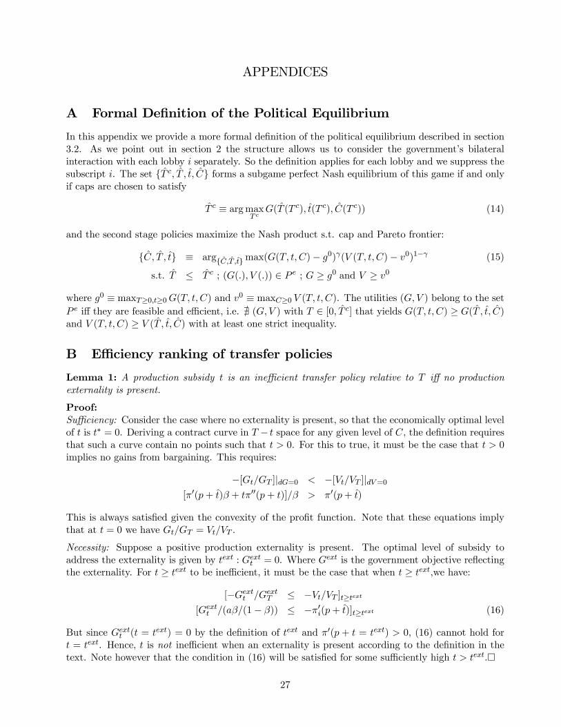
APPENDICES

A Formal Definition of the Political Equilibrium

In this appendix we provide a more formal definition of the political equilibrium described in section3.2. As we point out in section 2 the structure allows us to consider the government’s bilateralinteraction with each lobby i separately. So the definition applies for each lobby and we suppress thesubscript i. The set T c, T , t, C forms a subgame perfect Nash equilibrium of this game if and onlyif caps are chosen to satisfy

T c ≡ argmaxT c

G(T (T c), t(T c), C(T c)) (14)

and the second stage policies maximize the Nash product s.t. cap and Pareto frontier:

C, T , t ≡ argC,T ,tmax(G(T, t, C)− g0)γ(V (T, t, C)− v0)1−γ (15)

s.t. T ≤ T c ; (G(.), V (.)) ∈ P e ; G ≥ g0 and V ≥ v0

where g0 ≡ maxT≥0,t≥0G(T, t, C) and v0 ≡ maxC≥0 V (T, t, C). The utilities (G,V ) belong to the setP e iff they are feasible and efficient, i.e. @ (G,V ) with T ∈ [0, T c] that yields G(T, t, C) ≥ G(T , t, C)and V (T, t, C) ≥ V (T , t, C) with at least one strict inequality.

B Efficiency ranking of transfer policies

Lemma 1: A production subsidy t is an inefficient transfer policy relative to T iff no productionexternality is present.

Proof:Sufficiency: Consider the case where no externality is present, so that the economically optimal levelof t is t∗ = 0. Deriving a contract curve in T − t space for any given level of C, the definition requiresthat such a curve contain no points such that t > 0. For this to true, it must be the case that t > 0implies no gains from bargaining. This requires:

−[Gt/GT ]|dG=0 < −[Vt/VT ]|dV=0[π0(p+ t)β + tπ00(p+ t)]/β > π0(p+ t)

This is always satisfied given the convexity of the profit function. Note that these equations implythat at t = 0 we have Gt/GT = Vt/VT .

Necessity: Suppose a positive production externality is present. The optimal level of subsidy toaddress the externality is given by text : Gextt = 0. Where Gext is the government objective reflectingthe externality. For t ≥ text to be inefficient, it must be the case that when t ≥ text,we have:

[−Gextt /GextT ≤ −Vt/VT ]t≥text[Gextt /(aβ/(1− β)) ≤ −π0i(p+ t)]t≥text (16)

But since Gextt (t = text) = 0 by the definition of text and π0(p + t = text) > 0, (16) cannot hold fort = text. Hence, t is not inefficient when an externality is present according to the definition in thetext. Note however that the condition in (16) will be satisfied for some sufficiently high t > text.¤

27

C Proofs

Proposition 1: (Government cap on efficient transfers)Sufficiency:Suppose that γ ∈ (0, 1). We need only show the existence of a cap such that T c < TN andG(TNc, CNc) > G(TN , CN). The solution is illustrated in Figure 3. We first show that the con-strained Pareto frontier is strictly concave. On the basis of that, we then show that gNc > gN .The constrained Pareto frontier in Figure 3 coincides with the original one for T ≤ T c and thus itsslope is simply GT/VT up to point (CN , T c). From (6) we have GT /GC = VT/VC at (CN , T c) sothat GT/VT = GC/VC . The rest of the constrained frontier is strictly interior to the unconstrainedfrontier and has a slope of GC/VC , reflecting the ratio of changes in welfare as the amount of the lobbygood provided changes. Moreover, GC(CN)/VC = −Ψ0(CN) > −Ψ0(C < CN) = GC(C < CN)/VC ,from the definitions of G and V as well as Ψ00 < 0, so the constrained frontier is strictly concave.Now define point A in Figure 3 as the intersection of the constrained frontier and G = gN . Sincethe constrained frontier is strictly concave and gmc = gm for T c ≥ T 0 (see Figure 2), the segmentconnecting gm and A is everywhere below the constrained Pareto frontier.Consider then an auxiliary problem where the Pareto frontier is defined by the straight line throughgm and A, which has some slope m. For any linear Pareto frontier the government equilibrium utilityis gN − g0 = γ(gm − g0) (from (9)). Since the straight line through gm and A is a rotation of theoriginal Pareto frontier inwards around gm, and since gm − g0 and γ are unchanged in the auxiliaryproblem, the equilibrium government utility is also unchanged. Therefore if we derive the first-ordercondition for this auxiliary problem as we do for (8) we obtain −UV /UG|A = m. Strict concavity ofthe constrained frontier implies that at A, m > GC/VC |A, the slope of the constrained frontier at A.Therefore, the equilibrium point NC lies to the northwest of A, implying gNc > gN .

Necessity.If γ = 1 then the unconstrained solution is gm ≡MaxC,TG s.t. V = V 0 . The equilibrium transfer isTN(γ = 1) = T 0. A strictly binding cap entails that the government’s utility is now gmc ≡MaxC,TGs.t. V = V 0 and T c < T 0, the extra constraint implies that gmc < gm.If γ = 0 then the second stage Nash bargaining solution is GNc(TNc, CNc) = G(0, 0). The govern-ment is therefore indifferent among all values of T c, which implies that there exist T c ≥ TN (that is,caps that are not strictly binding) that are subgame perfect equilibria. ¤Proposition 2: (Government cap on efficient transfers and use of inefficient transfers)a. T c binds iff the government does not have all the bargaining power.In the political equilibrium T c must satisfy the following FOC: dG/dT c = 0, where dG/dT c ≡GCCT c+GTTT c+Gtt. Note that TT c = 1 since a marginal increase in the binding cap T c will inducean equivalent increase in the transfer. Thus, to show the gain from capping T , a proof similar to thatin Proposition 1 applies provided that the Pareto frontier is strictly concave when T c binds and t isavailable.The slope of the Pareto frontier is GT/VT if T c is not binding. If T c binds then any further increasesin the utility of the lobby must take place via changes in C being exchanged for t, since as we will seet > 0. Thus, if T c binds, the slope is (Gtdt −GCdC)/(Vtdt − VCdC) = Gt/Vt since the equilibriumdefinition requires t and C to be set efficiently, i.e. for Gt/GC = Vt./VC Therefore we have

limt→0Gt/Vt = GT/VT > [Gt/Vt]|t>0 (17)

where the first equality is due to the definition of G and V . (As shown in the proof of Lemma1 the utility frontier for efficient and inefficient transfers has the same slope when t → 0, that is

28

limt→0Gt/Vt = GT/VT .) The inequality follows from the definition of t being inefficient relative toT . Thus the constrained Pareto frontier is strictly concave around t→ 0 and we can apply the proofof Proposition 1 to show that T c binds.b. t > 0 in equilibrium.Suppose t = 0. Since T c is optimally chosen and binds the constrained solution would lie at thepoint where the new Pareto frontier meets the original one in Figure 4. However, since the uniqueunconstrained solution was t = 0, TN > T c and the slope of the frontiers is identical when t = 0 theconstrained solution cannot be T c, t = 0. ¤Proposition 3: (Government choice of inefficient policy as unique form of transfer)a. When γ = 0 we have G(0, tNt(γ), CNt(γ)) = G(TN (γ), 0, CN ) = g0. Equation (12) is thussufficient to show (10) is satisfied for γ ∈ (0, γ∗). To evaluate (12), we first use the implicit functiontheorem to obtain limγ→0 dg/dγ = limγ→0−LGγ/LGG where L is the Nash product evaluated at thesolution of the following program

MaxG≥g0L ≡ (G− g0)γ(Ω(G− g0))1−γ

The FOC LG = 0 is

γ(Ω

G− g0 )1−γ + (1− γ)(

G− g0Ω

)γΩ0 = 0

G− g0 = − ΩΩ0

γ

1− γ

Using this we have LGγ = L/ (1− γ) (G−g0) and LGG = [−γ/(1−γ)+(1−γ)Ω00(G−g0)2/Ω]L/(G−g0)2, which we use to obtain after some simplification

limγ→0 dg/dγ = lim

γ→0−LGγ/LGG = limγ→0−Ω/Ω

0

Therefore (12) reduces to (13) in the text.

b. At γ = 1 we have gm > gmt thus the government chooses T . Since the inequality is strict and Gis continuous in γ (G is continuous in the policies and (tNt(γ), CNt(γ)) and TN (γ) are continuous inγ) we can find a γ < 1 s.t. gN (γ) = gNt(γ). If (11) has a unique solution, then γ = γ∗. Otherwise γis the maximum γ that satisfies (11).¤Proposition 4: (Use of inefficient redistribution policies in a representative democracy)a. This follows from politicians having preferences G in (5) that are not perfectly aligned with eithervoting group. Since lobby goods initially have infinite value (that is, limC→0Ψ0(C) =∞), when a > 0and β < 1 there is a surplus to bargain over with each individual SIG in the second stage, as is clearfrom Figure 1.

b. If the two candidates are not extreme then whichever one is elected finds it optimal to use abinding cap on T and thus in equilibrium the inefficient policy is used as shown in Proposition 2. Ifthe candidates are extreme then neither will, if elected, have an incentive to restrict T thus t = 0, asshown in Proposition 2.¤Proposition 5: (Absence of transfers in direct democracy)a. Unorganized citizens do not benefit from transfers, but pay the taxes that allow them. Since notransfers imply no taxes, this is the preferred policy of all unorganized citizens. If they are in themajority,

Pi∈L αi < 0.5, then the policy of no transfers, either efficient or inefficient, will defeat all

29

other proposals in majority voting, independent of the identity of the politician in the second stage.

b. To show this we have to consider a number of cases: a policy of no transfers versus a policy ofT > 0 and t = 0 (the equilibrium outcome with no caps); a policy of no transfers versus a positivecap on T and t > 0; and a prohibition of T and t > 0. The different cases lead to different criticalvalues of the share of SIG voters, α, required for no transfers but for each case there exists a β suchthat the result holds. Since the intuition is the same, we derive it here only in the case prohibitingall transfers relative to allowing unrestricted efficient transfers T (so that t = 0).The welfare of the representative SIG is Vi. Voters in the SIG will prefer to prohibit transfers ifWi(T = t = 0) > Wi(Ti ∈ [T 0i , T 1i ], t = 0) − CTi , where the transfer is bounded by the value whenthe government has all bargaining power, T 0i , or none, T

1i . Using the definition of W (.) in (4) this

inequality becomes

li + π(pi) + αiNs > li + π(pi) + Ti + αiN [s−X

i∈L Ti/(1− β)N ]− CTi0 > Ti + αi[−

Xi∈L Ti/(1− β)]− CTi

If SIGs are identical then they supply identical goods, so that Ψi is identical for all i, which impliesCTi = CT . Since we assumed γ is the same relative to all i, we also have that Ti is the same forall i. Also, αi is identical across SIGs, so the same condition must hold for all SIGs. We may thenaggregate by summing over all i ∈ L, so that the above condition may be written asX

i∈L[Ti/(1− β)]X

i∈L αi >X

i∈L(Ti −CTi )X

i∈L αi > (1− β)(T − CT )/T ≡ αT (β)

where in the last line we use the fact that, when Ψi is identical across lobbies, T = Ti and C = Ci forall i. Note that conditional on transfers being approved by the majority the equilibrium for each Ti, Ciis independent of the number of lobbies (because of no lobby competition) or fraction of populationin lobbies, so the expression on the rhs is independent of αi and can be written as a function αT (β).We can then show that αT (β) ∈ [0, 1) by noting that, β ∈ (0, 1) and T ≥ CT . If T < CT the SIGwould choose not to bargain with the politician in the second stage since its utility would fall belowthe reservation value.¤

D Simulation

The following simulation shows that the condition in Proposition 3 can be satisfied so the governmentprefers production subsidies over lump-sum transfers when Ψ is sufficiently concave.Assumptions: Ψ ≡ Cψ,ψ ∈ (0, 1); q ≡ k1−αlα =⇒ π(p+ t) = (1− α)(p+ t)k((p+ t)α)

α1−α ,α = .5.

Slope condition for efficient transfer

limγ→0−Ω

T/Ω0T = limγ→0(V − v

0)Ψ0(CN) = (Tm − CN)aβ/(1− β) (18)

The first equality is due to the definition of Ω, the second is due to the first-order condition in (6).The last equality follows from the definition of V mT , where Tm represents the maximum transfer thelobby can extract and is defined by:

G(T = 0, t = 0, C = 0) = G(Tm, t = 0, CN)

Tm = Ψ(CN )/[aβ/(1− β)]

30

Using (18), Ψ and the solution to CN in (6) we obtain the general condition to be evaluated:

limγ→0−Ω

T/Ω0T = Ψ(CN )− CNaβ/(1− β)

= (1− ψ

ψ)aβ

1− βexp[(ψ − 1)−1 ln aβ/(1− β)

ψ] (19)

Slope condition for the inefficient transfer

limγ→0−Ω

t/Ω0t = limγ→0(V − v

0)Ψ0(CNt) = limγ→0(V

mT − v0)a(βπ0(p+ t) + tπ00(p+ t))(1− β)π0(p+ t)

(20)

The first equality, is due to the definition of Ω, the expression for Ψ0(CNt) in the second equalityis derived from the efficiency condition: Gt/GC = Vt/VC . Using the definition of V we obtainV mt − v0 = π(p+ tN(γ = 0))−Cmt − π(p) where Cmt is the minimum level of the good provided bythe lobby required to maintain the government at the reservation utility. Using the definition of Gand the condition G(T = 0, t = 0, C = 0) = G(T = 0, t = tN(γ = 0), Cmt) we can write Cmt as

Cmt = Ψ−1(−a(π(p+ tN (γ = 0))− π(p)− tπ0(p+ tN (γ = 0))/(1− β))) (21)

Using (20), Ψ, π(p+ t) and (21) we obtain:

limγ→0−

Ωt

Ω0t= [a(βπ0(p+ tN) + tNπ00(p+ tN ))

(1− β)π0(p+ tN )(π(p+ tN )− π(p)− Cmt)]γ=0 (22)

limγ→0−

Ωt

Ω0t= [a(βk

¡¡p+ tN

¢¢+ tNk))

(1− β)k (p+ tN)× 0.25(p+ tN )2k − 0.25p2k

− (−a(0.25(p+ tN)2k − 0.25p2k − 0.5tNk/(1− β)))1/ψ]γ=0

To calculate this we require the equilibrium t, which is obtained using the efficiency conditionGt/GC = Vt/VC and (21):

tN : Ψ−1(−a(π(p+ t)− π(p)− tπ0(p+ t)/(1− β))) = Ψ0−1(a(βπ0(p+ t) + tπ00(p+ t))

(1− β)π0(p+ t))

tN : (−a(0.25(p+ t)2k − 0.25p2k − 0.5tk (p+ t) /(1− β)))1/ψ = (1

ψ(a(βk (p+ t)α+ tk)

(1− β)k (p+ t)))−1/(1−ψ)

Evaluating (19) and (22) at the parameter values below we obtain the following:

limγ→0− Ωx

Ωx0ψ x = t x = T1/2 0.46 < 0.751/5 0.72 > 0.70Parameters: a = p = k = 1,β = 0.25,α = 0.5, γ = 0

Table 1: Simulation result for the choice of lump-sum versus production subsidies

31

32

Figure 1: Efficient Transfer

00 T 1T 0 T N

G = g 0

V = v 0

g m

v mC NN

G = g m

V = v m

Lob

by g

ood

Transfer

Figure 2: Cap on Efficient Transfer

00

N c

G = g 0

V = v 0

g m = g mc

v mN

v mc

G = g N

V = v N

T c

C c

T 0

Lob

by g

ood

Transfer

33

Figure 3: Bargaining Solution with Cap on Efficient Transfer

v m

g m =g mc

v N

g NN

A

U N = (G-g 0 )γ (V-v 0 )1-γ

N c

v Nc

g Nc

v mc

U Nc

g 0

v 0

G

V

Figure 4: Bargaining Solution with Inefficient Transfers

v m

g m =g mc'

v N

g NN

A'

U N = (G-g 0 )γ (V-v 0 )1-γ

N c'

v Nc'

g Nc'

v mc'

U Nc'

g 0

v 0

G

V

g Nc

34

Figure 5 Government's optimal redistribution policy

Figure 6 Bargaining power and the government's optimal

redistribution policy

g m

g N (γ<γ∗)N (γ<γ∗)

(G-g 0 )γ∗(V-v 0 )1-γ∗

v m

g mt

v mt

N (γ=γ∗)N t (γ=γ∗)

N t (γ<γ∗)g Nt (γ<γ∗)*

g Nt (γ=γ∗)*

=g N (γ=γ*)

G

Vg 0

v 0

A

g m

g N (γ<γ∗)

g mt

g Nt (γ<γ∗)*

γ10g 0

g Nt (γ=γ∗)*

=g N (γ=γ*)

γ∗

g Nt (γ)−g 0

g N (γ)−g 0 *

G

35

Figure 7: Bargaining Solution for caps in 1st stage

v m

g m =g mc

N = N b (γ1≤γ)

U N (γ)

N b (1=γ1>γ) = N c'

v Nv mc'

G

V

g Nc'

N b (1>γ1>γ)

U nc' (γ)

U Nb (γ1>γ)

g 0

v 0