Flow features in and around a (stented) coarctation features in and around a (stented) coarctation 1...

1

Flow features in and around a (stented)

coarctation

BMTE04.44

Marcel van ‘t Veer January 2004 – March 2004

Supervisors: - C.A. Taylor - F.N. Van de Vosse Abstract: A coarctation is a local narrowing of the aorta. It is a congenital disorder and therefore the treatment mainly concerns young children. The presence of a coarctation causes alterations in blood flow. Using an AutoCAD program to create a 3-dimensional geometry and a non-commercial intermediate program (Apsire2) to obtain meshes, a Finite Element Analysis of the blood flow is done. Several geometries like a stented coarctation and a non-stented coarctation are compared with respect to the flow features around the stent-struts and downstream of the coarctation. This gives insight in the influence of the presence or absence of a stent in the bloodstream with respect to the blood flow and velocity patterns.

M. van ‘t Veer Jan-Mar 2004

2

Flow features in and around a (stented) coarctation 1

1. Background and clinical practice ............................................................................ 3

2. Objectives................................................................................................................... 5

3. Methods...................................................................................................................... 6 3.1 SolidEdge........................................................................................................ 7 3.2 Apsire2............................................................................................................ 8

4. Results ...................................................................................................................... 10 4.1 Influence of the outflow tract........................................................................ 10 4.2 Influence of mesh refinement around the stent............................................. 12 4.3 Influence of the stent..................................................................................... 12 4.4 Influence of the coarctation .......................................................................... 13 4.5 Visualization of velocities and shear stresses at different cross sections ..... 13 4.5.1 Velocities .................................................................................................. 14 4.5.2 Shear stresses ............................................................................................ 20

5. Discussion................................................................................................................. 23

6. Conclusion ............................................................................................................... 24

Appendix A Check for mass conservation ............................................................. 27


3

1. Background and clinical practice Coarctations are a challenging condition seen in Pediatric Cardiology patients with congenital heart defects. A coarctation is a narrowing of a part of the aorta (fig. 1 and 2.A) thought to be caused by malformation of the media of the aorta. The prevalence of this pathology is about 6-8% in patients with congenital heart disease, which corresponds to 6 out of 10000 newborns. Evidence is available indicating there exist genetic factors associated with the development of a coarctation1.

Figure 1: Example of a coarctation before treatment. A left angulated (towards the head) view of the thoracic aorta and the aortic arch. The localized narrowing is clearly seen [J.A. Feinstein Pediatric Cardiologist, Stanford Hospital, Pediatrics-Cardiology].

The clinical presentation of a hemodynamic significant coarctation varies from asymptomatic high blood pressure or a little murmur, to heart failure and shock. In a significant number of cases the coarctation is a local narrowing of the proximal aorta. However there are variations in anatomy, physiology, treatment options and in outcomes. The narrowing develops primarily as a consequence of an abnormality of the media, thereafter intima proliferation occurs10. The prognosis is worse if coarctation presents itself in combination with other intracardiac pathologies like ventricular septal defects, bicuspid aortic valve, mitral stenosis, atrioventricular canal defects, d-transposition with or without tricuspid atresia, Taussig-Bing double-outlet right ventricle, and congenitally corrected transposition1. Some arteries (like the subclavian artery) may arise from or beyond the coarctation. As a consequence, these arteries can be narrowed at the ostium and so collateral circulation is needed to perfuse the tissue. This and other extracardiac pathologies like variations in the brachiocephalic artery can negatively influence the outcome of treatment1. The most conventional treatment of a coarctation is surgery1. Different techniques are available like using prosthetic patches after removing the narrowing, bypassing the whole stenosis2 with a bypass-graft or using body-own material to restore a normal pathway of the blood through the aorta. These techniques all require major surgery.


4

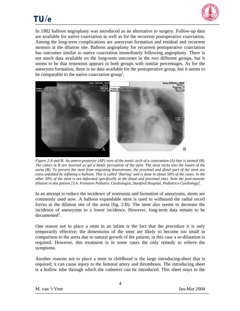
In 1982 balloon angioplasty was introduced as an alternative to surgery. Follow-up data are available for native coarctation as well as for the recurrent postoperative coarctation. Among the long-term complications are aneurysm formation and residual and recurrent stenosis at the dilation site. Balloon angioplasty for recurrent postoperative coarctation has outcomes similar to native coarctation immediately following angioplasty. There is not much data available on the long-term outcomes in the two different groups, but it seems to be that restenosis appears in both groups with similar percentages. As for the aneurysm formation, there is no data available for the postoperative group, but it seems to be comparable to the native coarctation group1.

B A

Figure 2.A and B: An antero-posterior (AP) view of the aortic arch of a coarctation (A) that is stented (B). The colors in B are inverted so get a better perception of the stent. The stent sticks into the lumen of the aorta (B). To prevent the stent from migrating downstream, the proximal and distal part of the stent are extra unfolded by inflating a balloon. This is called ‘flairing’ and is done in about 50% of the cases. In the other 50% of the stent is not deformed specifically at the distal and proximal sites. Note the post-stenotic dilation in this patient [J.A. Feinstein Pediatric Cardiologist, Stanford Hospital, Pediatrics-Cardiology]. In an attempt to reduce the incidence of restenosis and formation of aneurysms, stents are commonly used now. A balloon expandable stent is used to withstand the radial recoil forces at the dilation site of the aorta (fig. 2.B). The stent also seems to decrease the incidence of aneurysms to a lower incidence. However, long-term data remain to be documented1. One reason not to place a stent in an infant is the fact that the procedure it is only temporarily effective; the dimensions of the stent are likely to become too small in comparison to the aorta due to natural growth of the patient; in this case a re-dilatation is required. However, this treatment is in some cases the only remedy to relieve the symptoms. Another reasons not to place a stent in childhood is the large introducing-sheet that is required; it can cause injury to the femoral artery and thrombosis. The introducing sheet is a hollow tube through which the catheters can be introduced. This sheet stays in the


5

femoral artery during the procedure. A valve in the sheet prevents blood from flowing out of the artery.

2. Objectives There is little understanding about the development of the (re-)coarctation after a treatment in cases of surgery, stenting or angioplasty3. The only parameters that are measured in clinical practice are pressures in the aorta and the pressure gradient over the stenosis before and after the percutaneous procedure. Also a global impression of the geometry is obtained by making aortograms before and after the procedure4. The goal of the intervention is to minimize the pressure gradient. To obtain follow-up data a diagnostic catheterization has to be done and an introducing sheet has to be brought in place. Obviously, if a patient is asymptomatic, no re-catheterization takes place. This is one reason why there is little long-term follow-up data on native coarctation stenting as well as on recurrent post-operative coarctation stenting1. Several studies have shown that sites that are exposed to non-physiologic values of shear stress for a longer period of time can develop diseases like atheroscleroses5. A related problem, which is also due to atheroscleroses, is the formation of aneurysms. The shear stress is related to velocity gradients in the flow and therefore evaluation of the flow should be useful. The flow has an impact on the function of the individual endothelial cells in the vessel6. This is indirectly related to the outcome the patient. To gain more insight in the shear stress distribution and the flow features in the stented coarctation simplified models of the aorta were made and Finite Element Analysis was performed using the models. Velocities and the related shear stress in the model are evaluated and compared to a model of a non-coarcted vessel. The overall goal of the use of these models was to gain better insight in the physiology of a coarctation and assess the influence of different geometries on blood flow. Not only will the coarctation alter the flow, the stent itself can also cause disturbances. The effect of a certain stent design can easily be explored with these models by comparing a stented with a non-stented situation. It is known that stents that are placed in a coarctation can migrate downstream. In some cases the stent sticks into the lumen of the vessel (fig.2.B). This is a reason to deform the proximal and distal part of the stent, ‘flairing’, with a balloon to prevent it from migrating. As a matter of fact, such additional problem might also affect shear stress patterns. However, there is no consensus on flairing the stent or not. In half of the cases the stents are flaired and in the other half, they are not. The simplified model can give more insight in the flows and shear stresses of the two different cases. This study will not give direct answers to the questions that exist in the clinic like: why does the blood pressure still reach pathologic high values at exercise even after eliminating the pressure gradient of the coarctation? And: will “flairing” the stent improve the long-term outcome of the treated coarctation? However, it will give insight in the flow phenomena that appear in and around a (stented) coarctation. These results can be used for more advanced models with realistic geometries for instance.


6

3. Methods A wide variety of different configurations after stent placement is seen in patients because of different anatomical and physiological characteristics of each coarctation. Possible configurations include an over-expanded (fig. 3.A) or an under-expanded (fig. 3.B) stent. The reason to over-expand a stent is to compensate for anticipated possible neointimal narrowing. In some cases the balloon cannot be inflated to the preferred size. There might be a risk of tearing the aortic wall open. In such a case the interventional cardiologist may decide to re-dilate in a later stadium. This configuration of an under-expanded stent is also seen in the case where the stent has become small in comparison to the aorta due to the natural growth of the patient, as mentioned before. It is important to realize that an angioplasty is intended to tear several parts of the aortic wall, but in a controlled way.

Figure 3.A and B: Model of a representation of an over-expanded (A) and an under-expanded (B) stent in a coarctation. Made with the AutoCAD program SolidEdge.

A B

A related configuration of the under-expanded stent can be observed when the stent is too long in comparison to the coarctation (fig. 2.B); a simplification of the case showed in figure 4.A. The proximal as well as the distal part of the stent are likely to stick into the lumen of the aorta, which is sized normally. The stent alters the blood flow in the vessel. The related shear stress can have long-term consequences5 but also an acute complication. In clinical practice it appears that stent can wash out of the coarctation as a consequence of the shear stresses acting on the stent. The migrated stent can cause complications downstream and surgery is inevitable.

Figure 4.A and B: Representation of the coarctation with the stent sticking into the lumen (A) and the flaired variant of this configuration (B). Made with the AutoCAD program SolidEdge

A B


7

In this study this configuration of the stent that sticks into the lumen of the vessel (fig.4.A) was of interest and all the simulations were done in relation to this configuration. To gain more insight in the shear stress distribution and the flow features in and around this stented coarctation (fig.4.A), in essence three simplified numerical models of the aorta were made and Finite Element Flow Analysis was performed using these models. An analysis was done on a model of a normal aorta, represented by a straight tube. The model of the normal aorta was compared to a model of a stented coarctation in which the stent was sticking into the lumen. A third model was made, which represented the coarctation without the stent. In principle the model was the same, except for the stent, which was not present in the model. It should be emphasized that it was not the intention to model a realistic morphology in this case. The purpose of this model was to assess the influence of the stent on the flow in comparison to the flow in the stented coarctation. The parameters that were analyzed for all the models were velocities and shear stresses. As mentioned before, to prevent the stent from migrating, the proximal and distal part of the stent can be deformed. This is called ‘flairing’. A representation of a flaired stent is drawn in figure 4.B. There is no consensus on the best treatment of the aorta if the stent appears to have this configuration. In half of the cases the stents are ‘flaired’ and in the other half, they are not. A simplified model can give more insight in the flows and shear stresses of the two different cases. However this is beyond the scope of this report. No numerical model was made of this configuration and no Finite Element Analysis was done on this configuration. The 3D-geometries were drawn in an AutoCAD program called SolidEdge® (Version 10.00.00.50 ©2001 UGS). These drawings like figure 3 and 4 are just simplified graphical representations of real configurations. An intermediate program, called Apsire2 (Version March 26 2004 © 1998-2003, Stanford University), was used to convert these drawings to numerical models. Apsire2 was also used to generate meshes by calling MeshSim (Version 5.2) (a meshing program). A mesh consists of elements that describe the 3D-geometry. The meshes were necessary to calculate velocities and shear stresses. Apsire2 also created files that were necessary for the Finite Element Analysis. The actual analysis was done on another computer that used SPECTRUM (Centric) as a solver. The program could run in a parallel circuit of processors to reduce the calculation time. 3.1 SolidEdge The lumen of the vessel that remains after implantation of the stent is the volume that is modeled. The initial geometries were three cylinders that were connected (fig.5.A). To draw a somewhat more realistic representation than just three joining cylinders, the edges of the coarctation were rounded (fig.5.B). The dimensions of the model are shown in millimeters in figure 5.A. The stent itself was cutout of the volume. The result is a simplification of a Palmaz (Johnson & Johnson) stent (fig.4.A), commonly used in the treatment of a coarctation. The dimensions of the models are in the physiologic range. The diameter of the stented coarctation is 15 mm and the diameter of the normal aorta is 20 mm. The length of the coarctation is 15 mm.


8

Figure 5.A and B: Different stages in the development of the realization of the model. In A the dimensions of the model are given in millimeters. The inflow-tract as well as the outflow-tract is 45 mm in length. In B the edges are rounded to achieve a more realistic geometry. 3.2 Apsire2 The SolidEdge-model was exported as a Parasolid file and read in into Apsire2 (Version March 26 2004, © 1998-2003 Stanford University). The volume was divided up into elements using the mesh-generator option in Apsire2, MeshSimm. The Global Maximum Edge Size (GMES) specified the element size. The GMES was related to the number of elements; the smaller the GMES the bigger the number of elements (fig. 7). The model consisted of linear tetrahedral elements. The different boundaries were specified in Apsire2. For each model there were three different boundaries namely an inflow-boundary, an outflow-boundary and the wall. For these three faces, boundary conditions were specified. For the inflow-boundary a physiological flow was applied. This volumetric flow (fig. 6) was obtained from different experiments and represents the suprarenal aortic flow in a normal aorta with a diameter of 2 cm. For the wall a non-slip condition was applied. Zero pressure was assumed at the outlet. For an entrance flow, the Womersley solution was selected. The Womersley solution is the analytical solution of the Navier-Stokes equations for pulsatile flow. By knowing the volumetric flow that is entering the vessel and the period of the cardiac cycle, the velocity-profile for the entrance can be obtained. This solution is a good approximation to the real flow-patterns in the aorta, although assumptions have been made to calculate this Womersley-solution; blood was treated as an incompressible and Newtonian fluid, the vessel wall was rigid and the flow fully developed and laminar.


9

Figure 6: The volumetric flow used as the input flow in the coarcted models. With Apsire2 the Womersley solution is calculated as the input velocities at every nodal point at the inflow-face of the mesh. This is a representative flow pattern for a normal suprarenal aorta. The computer (128-processor Origin 3800, SGI in Mountain View), which was used for the calculations, had several processors to save time solving the Navier-Stokes equations for the model. The solution was obtained by integrating with a time-step of 0.004 seconds, so at 200 time points in the cardiac cycle. The results were generated every 10 time-steps (“*.vis”-file) i.e. 20 images per cardiac cycle.

A B

Figure 7.A and B: Two different meshes of the model with the stent sticking into the vessel lumen on both sides of the coarctation. The Global Maximum Edge Size in A is 3(50.000 elements) and in B 0.5 (approximately 1 million elements). Using the geometry and the flow input, a typical Reynolds number of about 600 can be calculated.


10

4. Results The *.vis-files were imported in Apsire2. To visualize velocities and shear stresses, options like contour-plots, vectors-plots, and warp-vectors were available. Contour-plots represent the magnitude of the axial velocity (in colors) but do not specify the direction in which the vector is pointing; vectors-plots cover this property. Vectors represent the magnitude of the velocity or the shear stress as in colors as well as in the size of the vector. Warp-vectors merge vectors and the velocity is represented by a moving, colored surface (over the top of the vectors). Information to obtain the separate flow-directions of points is lost but it will give a good representation of the velocity profile at cross section of the vessel. In the following part of this report several numerical models will be presented. Each of the models is the next step in the process to obtain reasonable results from the simulation. The first model seemed to have an outflow-tract that was too short (model 1, 4.1). The graphical representation that was used to construct the model is drawn in figure 4.A. The solution was not stable and the simulation stopped. The next step was to extend the outflow-tract (model 2, 4.2) to avoid this problem of an unstable solution. The outflow-tract was extended by a factor 7, which was arbitrary. As a result this model had an outflow-tract that was 300 mm. Subsequently the next step was to resolve more flow-features around the stented coarctation. For this purpose the mesh was refined around the stent (model 3, 4.3). To assess the influence of the stent on the flow, a simulation without the stent modeled in the coarctation (model 4 (4.4)), was done. Finally, to exclude that any flow-features would appear in a straight tube, model 5 (4.5) was made. 4.1 Influence of the outflow tract 4.1.1 Outflow tract too short For this simulation the mesh with over one million elements was used. The simulation results consisted of velocities with a magnitude and a direction at every nodal point. As mentioned above at the outlet a zero-pressure condition was applied. However, if the results from the equations do not match with the zero pressure at the outlet, a solution can diverge. As a result in the case of a complex vortex the pressures are not equal over the cross section. To still maintain this zero pressure, the solver introduced arbitrary velocities. The error became rapidly larger and the solution diverged (fig. 8a-d). To overcome this problem the outflow-tract was extended.


11 M. van ‘t Veer Jan-Mar 2004

Figure 8.a-d: Vector representation of the velocity in a longitudinal cross section of the coarcted model with the stent sticking into the lumen. The white arrow next to the models represents the direction of the flow. Blue color and little vectors correspond to low velocities (small magnitudes) and red and large vectors correspond to large velocities. Beginning of systole (a); instantly after the beginning of the heart-cycle the velocity increases in the narrowed area as a result of the rigid wall. Behind the stenosis complex vortices develop (b and c). The solution is diverging and increasing velocities are seen on the outflow face (d).

dcba

4.1.2 Long outflow tract To prevent the model from diverging, a new geometry was drawn in SolidEdge. The outflow-tract was extended from 45 mm to 300 mm to let the flow develop and let it come to a steady state (fig. 9.A). However this arbitrary extension is maybe too long, the problem of diverging was solved. After exporting it as a Parasolid and meshing it in Apsire2, a new simulation was started with the same boundary conditions as in the previous case. The mesh consisted of about one million elements with a GMES of 1 (fig. 9.B).

Figure 9.A and B: Extended model in SolidEdge (A) and meshed (B). The mesh consists of over 1 million elements. The outflow-tract is extended from 4.5 cm to 30 cm.

B A

As with the non-extended model, the velocities can be represented as (warp)vectors or just as colors representing the velocity. To compare the results with different models, the results are shown under section 4.5. Both velocities at different cross sections and shear stress on the wall of the model are plotted.

12

4.2 Influence of mesh refinement around the stent To increase the resolution and by doing so resolve more flow-features, the GMES had to be smaller and in consequence more elements were generated. However, the flow features in the large part of the outflow tract were of little interest and therefore did not need to have this fine resolution. An option in Apsire2 was used to specify smaller GMES-es at specified faces. The result at the outer surface is shown in figure 10. The elements become larger to the inside of the vessel; this is showed in a longitudinal cross section in figure 11. This model consisted of about two million elements.

Figure 10: Close-up of the refined mesh around the stent. Locally the GMES size is 0.2 where the rest of the model had a GMES of 1. Locally the flow features should be better resolved.

Figure 11: Longitudinal cross-section of the refined mesh; close-up of the part where the stent is located. Only the outside faces have the really fine mesh; towards the middle of the vessel the mesh has the same refinement as the rest of the model. However, around the stent-struts the mesh is also fine.

Apart from the better resolution around the stent, the rest of the model also consisted of more elements than the extended model without the refinement around the stent. The velocity and shear stress results are shown under section 4.5. 4.3 Influence of the stent Flow is altered by the stent and also by the coarctation. To verify the influence of the stent on the flow features, a model was made without the stent cut out of the lumen. To


13

maintain the same model in principle, this model was refined around the coarctation too. The surface mesh is shown in figure 12.A and a longitudinal cross section of this model without the stent is shown in figure 12.B. As like for the rest of the models, the results are shown under section 4.5.

A B

Figure 12.A and B: Surface-mesh of the model without the stent (A). Note the refinement around the coarctation. A longitudinal cross section of this model (B). Note that the mesh-refinement is also in this model just present on the surface.

4.4 Influence of the coarctation As a control, a simulation was done with a straight tube with the same length as the extended models but without refinement and without the (stented) coarctation . Because a Womersley-profile is used as an entrance-flow profile, the expected solution for the whole tube should be the same Womersley profile as at the entrance. As mentioned before, the analytic solution of a pulsatile flow through a straight rigid tube with a laminar, developed flow and an incompressible Newtonian fluid equals the Womersley solution. 4.5 Visualization of velocities and shear stresses at different cross sections Images were made throughout the cardiac cycle at every 10 time-steps (40 milliseconds) of the simulation as mentioned above. To compare the different models, cross sections at specific locations were made to assess the velocities. Both (warp)vector-plots and contour-plots were made of cross sections perpendicular to the axial direction of the model, just distal to the stent and somewhat more downstream where flow alterations were expected. Longitudinal cross sections are made of each model and vector-plots and contour-plots were made to assess and compare the flow-features. At regions of interest, like around the stent (coarctation) and downstream of the coarctation, close-ups were made. The shear stress was examined as mean shear stress and as the instantaneous shear stress. Mean shear stress is the “mean over the cycle” at every point at the surface and plotted as a contour-plot. For the shear stress a global impression was obtained by looking at the whole model. The instantaneous shear stress was also plotted for different locations and for different time-steps.


14

4.5.1 Velocities A longitudinal cross section reveals a global overview of the magnitudes of the velocities in that plane. However, no information of the direction of the local flow can be distinguished. Features like secondary flows as in swirling and turbulence can be

Figure 13.A-D: Velocity in systole in the different models; straight tube (A), non-refined extended and stented coarctation (B), refined model around the stent (C) and the model without the stent (D). The white arrow indicates the main direction of the flow. Of course no secondary flows are observed in the straight tube because this is just a representation of the Womersley solution. Slight differences in maximum velocity can be seen between B and D and C and D.

calized. For the straight tube, no changes in the axial direction are observed and

decelerates again and in all models, except of course for the

lotherefore the maximum velocity at every cross section perpendicular to the flow direction (axial) equals the maximum velocity at the inflow, which is about 0.5 m/s (fig. 13.A). Flow accelerates trough the coarctation obviously and velocities of about 1 m/s are observed (fig.13.B-D). After diastole the flowstraight tube, swirling of the blood appears. For example in mid-diastole (fig. 14), which is at about 2/3 of the cardiac cycle, in a large part of the outflow-tract the flow is swirling. (fig.14.B-D). Flows are low but information on the direction of the flow cannot be gained from figure 14. A white arrow indicates the main flow direction in the following figures.


15

Figure 14.A-D: Velocity in diastole in the different models; straight tube (A), non-refined extended and stented coarctation (B), refined model around the stent (C) and the model without the stent (D). The white arrow indicates the main direction of the flow. Again, no secondary flows are seen in the straight tube. In B the flow seems to differ from C and D. At the same time point (at 70 % of the cardiac cycle) somewhat higher velocities are seen in the more resolved models.

To look at the directions (and magnitudes) of the velocities, both vector-plots and

en the non-refined (fig.15-16.A and D) and

contour-plots are made of regions of interest are made of the same longitudinal cross sections. Both the areas around the stent and just distal to the stent (fig.15 and 16) as well as the swirling region (fig 17) are of interest. Differences in the flow-pattern are seen betwethe refined model (fig.15-16.B and E) along the cardiac cycle. These figures show that the stent-struts influence the flow-pattern compared to the non-stented model (fig.15-16.C and F).


16

Figure15.A-F: Close up of the (stented) coarctation of the three different models in systole; the extended non-refined model (model 2) with stent (A and D), refined model with stent (model 3) (B and E) and the model without the stent (model 4) (C and F). The white arrow indicates the main direction of the flow. Contour-plots (A-C) and vector-plots (D-F) of the models at the same time point in the cardiac cycle. A to C give a global overview of the flow magnitudes. The places where the struts of the stent are present in the vessel are clearly seen in A, B and D. Because of the refinement of the mesh, vectors cover this stent-strut in E. In all of the models back-flow just distal to the coarctation, next to the wall, appears (D-F). There are slight differences in the position where they occur. There are also differences in the amount and magnitude of this back-flow. Also, low but significant velocities are seen in the stent just distal to the stent-struts in E that are not present in D. As mentioned in figure 13, the maximum velocity (seen in the middle of the coarctation) in F is lower than in D and E.

Figure 16.A-F: Same as figure 15 but in early diastole. The black arrow indicates the direction of the main direction of the flow in the models. There are differences around the stent and the stent-struts between A and B. Larger areas of back-flow can be obtained (D-F) with differences in area and magnitude among the models. Small flow-features are obtained around the stent in E that are not present in D (light blue spots).


17

Figure 17.A-F: Close up of the swirling in the three models. The white arrow indicates the direction of the main flow-direction. Both the contour-plots and vector-plots are representing the same time step in the cardiac cycle (early diastole). As mentioned before, there are qualitative differences between the three models; the differences in magnitude can easily be seen in A-C as for the differences in backflow D-F are useful.

The perpendicular cross sections of the models are made at specific places. The first cross section is made just distal of the stent (fig 18). The other cross section is made more distal where the swirling occurs (fig. 19). The results of the velocities of the cross section just distal to the stent are seen in figure 20 as a contour-plot. In figure 21 the velocities are represented as warp-vectors. Contour-plots and vector-plots of the swirling-sites are presented in figure 21 and 22.

Figure 18: Cross section for assessing the velocity just distal from the stent. The

rface-mesh is helpful for

orientating. The arrow indicates the

direction of the flo

Figure 19: Cross

section at the swirling site, more distal from the stent. The

arrow indicates the direction of the flow.

su

w.


18

Figure20.A-D: Contour-plot representation of the velocity in systole in a cross section just distal to the stent. The four different models are shown; straight tube (A), extended non-refined stented coarctation (B), refined model around the stent (C) and the model without the stent. It is clearly seen that the maximum velocity in the presence of the stent (B and C) is higher than in the other models. The stent struts seem to have an impact of the shape of the flow profile because of the non-circular shape of the velocity profile seen in B and C in comparison to A and D.

Figure 21.A-D: Warp-vector representation of the velocity in systole in a cross section just distal to the stent of the four models in the same order as in fig. 17. The white arrow in the middle indicates the direction of the main flow. The same observations as in fig. 17 can be made with respect to the circular shape of the non-stented and the non-circular shape of the stented model with respect to the velocity profile. The profile in A has a somewhat rounder shape than the shape in D (note that the colors are inverted; the high velocities are represented as blue and the low velocities as red), which looks more like a plug-flow in the center of the vessel. The colors in B and C are also inverted, but nevertheless the profile in C seems to be a more accurate representation of the actual velocity field trough the stent because of its symmetry.


19

In the same order the results for the swirling site are obtained but in a different time in the cardiac cycle. In figure 22 the color plot of the cross section in the swirling-site is shown and the vector representation is shown in figure 23 to examine the direction of the secondary flows. These results are in mid diastole at 2/3 of the total cardiac cycle.

Figure 22.A-D: Contour-plots of the velocity perpendicular to the axis of the model distal from the stent (see fig.19). (The order of the results is the same as the previous two figures). As expected, there are no secondary flows present in A. It seems however that there exist more complex secondary flows in the cases with stent (B and C) than in the case without the stent (D) at this time-step.

Figure 23.A-D: Vector-plot of the velocity perpendicular to the axis of the model far distal from the stent. (The order of the results is the same as the previous figures). The white arrow indicates the direction of the main flow-direction. The velocities of the nodal points point in different directions in this fase of the cardiac cycle; in A where the center velocities are pointing forward and the velocities close to the wall are pointing backward. This is also obtained in B-D but more complex flows appear and the velocities are of larger magnitude. There is a difference between the cases with stent (B and C) and

without stent (D); the velocities seem to have larger values in the presence of a stent.


20

4.5.2 Shear stresses As mentioned earlier, the mean shear stress is the mean over the cardiac cycle and it allows one to get an impression which areas in the vessel are subjected to high and which to low values of shear stress (fig. 24). The values are in dynes/cm2 (1dynes/cm2= 0,1 Pa) and for the mean shear stress the range is between the 0 and 5 dynes/cm2. Throughout the cardiac cycle the instantaneous shear stress changes and in figure 25-28 different steps of the cardiac cycle are represented in a close-up of the area just distal to and at the stented coarctation. These are vector-plots and in consequence the direction of the shear stress can be obtained. The shear stress plotted is the reaction force to the flowing of the blood, so it is opposite to the direction of the flow.

Figure 24.A-D: The mean shear stresses on the wall of the four models. There is no disruption in the shear stress distribution of straight tube (A) (which was expected). Globally the shear stress distribution in the remaining models is the same. There are high shear stresses near the inflow of the coarctation and also in the (stented) coarctation. Furthermore, the area just distal of the coarctation is exposed to low shear stresses. However there are slight differences in the distribution downstream. Locally values of about 5 dynes/cm2 are observed in the stented models (B and C) in comparison to D.


21

For the instantaneous shear stress just distal to the coarctation only the coarcted models are shown. Note that the range for the instantaneous shear stress is from 0 to 10 dynes/cm2. The different time-points of the cardiac cycle are at systole (1/2 of the total cycle (fig. 25)) and at early diastole (2/3 of the total cycle (fig. 26)). Shear stress is derived from the velocity. Because of the inversed flow along the wall just distal to the coarctation, the shear stress is also reversed. For the different time-points in the cardiac cycle, the results show that the area of the reversed shear stress (red area in figure 25 and 26), migrates downstream. However, among the models differences appear in the distribution of this area of high shear stress. The difference can be explained because the velocity solutions differ among the models.

Figure 25.A-C: Instantaneous shear stress just distal to the coarctation in systole (1/2 of the cardiac cycle). The white arrows indicate the direction of the main blood-flow. Both for the stented (A and B) as for the non-stented (C) models a large area of reverse shear stress appears just distal to the coarctation (red area). Differences in the areas of high shear stress can be observed among the models.

Figure 26.A-C: Instantaneous shear stress just distal to the coarctation half way in diastole (2/3 of the cardiac cycle). The white arrows indicate the direction of the main blood-flow. The non-refined model (A) shows a different distribution of the shear stress and more small areas of high shear stress are obtained than in the refined model (B) and the model without the stent (C). The areas of high shear stress in B and C are comparable in size but slightly differ in shape.


22

For the instantaneous shear stresses around the stent, the range for the shear stresses is from 0-15 dynes/cm2. The scaling of the vectors is adjusted because of the fine mesh in this area; else the vectors would overlap. Two different phases of the cardiac cycle are selected; systole and mid-diastole (fig.27 and 28). Obviously differences in the distribution of the shear stress are seen. The shear stress is distributed more regular in the cases without the stent (27.B and 28.B).

Figure 27.A and B: Instantaneous shear stress of a close-up of the stented and non-stented coarctation in systole. The white arrows indicate the direction of the main blood-flow. Obviously there is a difference in instantaneous distribution of the two different models. The stent seems to experience large shear stresses (A). In both models the geometry of the vessel seems so induce large shear stresses (inflow of coarctation (A and B)).

Figure 28.A and B: Instantaneous shear stress of a close-up of the stented and non-stented coarctation in mid-diastole. The white arrows indicate the direction of the main blood-flow. Between the struts of the stent there are local high shear stresses (A) in comparison to the same locations in the non-stented model (B).


23

5. Discussion In this project numerical research was done on flow features as a consequence of the presence of a stent. The small flow alterations around the stent struts are thought to be important in the development of for in-stent restenosis7. To describe these flow features accurately, the mesh has to be fine enough. The simulations between the non-refined and the refined mesh show that the exact solution was not yet achieved in the non-refined model. An even finer mesh is needed to rule out the possibility that the solution was significantly different from the refined mesh. If the solution would not be significantly different, the amount of elements can be maintained to prevent long calculation times. The presence of a stent matters for the flow-patterns as shown in the different simulations. However, these results only show qualitatively differences between the models. For different designs of stents, this relatively simple simulation can be done to obtain the induced flow alterations. For instance, biodegradable stents have bigger struts and will in consequence alter the flow more. But also the geometry can matter and this idealized model is useful to look at the differences between the stents in the flow disturbance and maybe even the total force that acts on the stent that can cause it to migrate downstream. The same analysis should be done on a ‘flaired’ model with and without stent to obtain differences in these configurations. As seen in this study, complex flow-patterns develop downstream of the coarctation. Similar results are reported in literature9. But also the geometry influences the results of the simulation. Apart from a narrowing, curvature of the vessel influences the flow-patterns as well8. To relate the results to more patient specific problems, more realistic models of the aorta and the coarctation have to be made. Attention has to be paid to the boundary conditions applied in the models because these can have major impact on the results. Inflow-velocities as well as the geometry of the vasculature can be acquired by MRI. The maximum velocities in these models at the inlet were as low as 0.5 m/s due to the used volumetric flow. The suprarenal flow is less than the thoracic aortic flow, where the coarctation is located, due to branches that go of the aorta. In a normal thoracic aorta this velocity is twice as high. Flow patterns of even higher velocities can be of interest to assess the influence of exercise. The fact that there is no mass conservation could also account for the inaccuracy of the solution. Therefore a check for mass-conservation is done by looking at the percentage in difference between the inflow and outflow of the model. The results are shown in Appendix A. The percentages for the three different models are: -0.0139% for the extended non-refined model, 0.0028% for the refined model and 0.0116% for the model without the stent. These percentages (relative to the inflow) are small and therefore the conclusion can be drawn that the solution was not affected by the fact there is no mass conservation. The little differences are due to the fact that the solution is numerical. The implementation of biological models that cover the cell-response to local hemodynamics6 may answer questions that arise in the following cases. One of the


24

problems seen in clinical practice that cannot easily be explained, is that after the treatment no gradient is present, but some cases exercise tolerance stays still low. Blood pressure will reach pathologic high values with all consequences. The pressures are of great interest as follows from these examples. This project was focused on the flow-patterns and the shear stress and in consequence no pressure information was obtained. However, to get better understanding of specific cases, future work should include pressures or pressure gradients.

6. Conclusion The results for the straight tube are as expected, because this had to be the solution for Womersley profile. No differences in the longitudinal directions are seen because the velocity only differs with the radius and is independent of the longitudinal coordinates in this solution. There are some differences between the two stented models (the non-refined and the refined model). It seems that the solution that is obtained from the non-refined model has not reached a solution that resolves all the small flow-features; it is not the ‘exact’ solution. The differences between this model and the refined model differ for instance in the perpendicular cross section just distal to the stent. This suggests that indeed the non-refined model was not sufficient enough in resolving the small flow features. The cross sections presented as warp-vectors show that the solution of the refined model is more symmetric than the non-refined model, which might suggest also that the results are not fully reliable. Moreover the small flow features around the stent-struts and the features at the vessel wall at the site of the stent are not sufficiently accounted for by the non-refined model. These can be observed in the refined model. Little spots of backflow are seen around the stent-struts in the coarctation that are more difficult distinguished in the non-refined model. The ability to resolve most of the flow-features is missed by the non-refined model. Globally the same swirling occurs at about the same location downstream of the coarctation in the non-refined model, the refined model and the non-stented model. The swirling is quite random and, as a consequence, difficult to analyze in qualitative as well as in a quantitative way. The differences between the refined stented model and the model without the stent are also best observed in the perpendicular cross sections just distal to the stent. In the presence of the stent a star-like profile is observed in the cross section. The stent obviously has influence on the local flow-features around or near the stent. These features are not seen in the model without the stent. The flow-pattern in the center of the vessel just distal to the coarctation looks more like a plug-flow in the non-stented model than in the stented one. Furthermore the maximum velocity in the presence of the stent is higher than in the absence of the stent. This can have to do with the fact that the stent occupies space in the lumen and therefore the velocity has to be higher. The effect of a certain stent design can easily be explored with these models by comparing a stented coarctation with a non-stented one.


25

Without doubt there is a constant value of mean shear stress over the surface of the tube in the case of the straight tube. Again, the three models (non-refined, refined and non-stented model) show globally the same features; low shear stress region just distal to the stent, high shear stresses at the entrance and in the (stented) coarctation and randomly distributed shear stress regions of high and low values down stream the coarctation. Quantitatively differences cannot be observed. For the instantaneous shear stresses the same global features are seen except for the distribution of the shear stress in diastole, which is randomly distributed. This has probably to do with the fact that the solution is not the ‘exact’ solution and because of the fact that shear stress is a derivative quantity and therefore extra sensitive for errors in the flow solution.

Acknowledgements: Within the framework of my Master-phase of Medical Engineering (University of Technology Eindhoven) I had the opportunity to do my internship abroad at the Cardiovascular Biomechanics Research Laboratory in Stanford. I would like to thank Nico Pijls, cardiologist at the Department of Cardiology Catharina Hospital Eindhoven, for making this internship possible. And I also would like to thank everyone from the lab for an unforgettable time in and outside the lab. I really want to thank Charles Taylor for the hospitality and the possibility to get to know a lot of people and learn a lot of new things.


26

7. References

1. Moss and Adams’, Chapter 49: Coarctation of the aorta, Heart Disease in Infants, Children, and Adolescents, © 2001 Lippincott Williams & Wilkins.

2. Heidi M. Connoly, MD, Hartzell V. Schaff, MD et al. Posterior Pericardial Ascending-to-Descending Aortic Bypass, Circulation. 2001; 104[suppl 1] I-133-I137.

3. C. Zabal, F. Attie et al. The Adult Patient with Native Coarctation of the Aorta: Balloon Angioplasty or Primary Stenting? Heart 2003; 89: 77-83.

4. B.D. Thanopolous, L Hadjinikolaou et al. Stent Treatment for Coarctation of the Aorta: Intermediate Term Follow Up and Technical Considerations, Heart 2000; 84; 65-70.

5. C. Zarins, M.Zatina, D.Giddens, D. Ku and S. Glagov. Shear stress regulation of artery lumen diameter in experimental atherogenesis. Journal of Vascular Surgery 1987; 5: 413-420.

6. P.F.Davies, J. Zilderberg, B.P. Helmke, Spatial Microstimuli in Endothelial Mechanosignaling, Circulation Research 2003; 92: 359-370.

7. Frank, A.O., Walsh, P.W. et al. Computational fluid dynamics and stent design, Artificial organs, Jul 2002; 26:614-621

8. Long, Q, Xu, X.Y. et al. Numerical investigation of physiologically realistic pulsatile flow trough arterial stenosis. Journal of Biomechanics, Oct 2001; 34, no.10: 1229-1242.

9. Y. Niu, W. Chu, et al. Numerical evaluation of curvature effects on shear stresses across stenoses. Biomedical Engineering, Applications Basis Communications; Aug 2002; 14, no.4: 164-170.

10. T.W. Sadler, P.W.J. Peters, Langman’s medische embryologie en teratology. 2000 Houten/Diegem, Bohn Stafleu van Loghum.


27

Appendix A Check for mass conservation

percentage_mass_diff_extended_model = -0.0139% percentage_mass_diff_without_stent = 0.0116% percentage_mass_diff_refined_model = 0.0028%


Flow features in and around a (stented) coarctation features in and around a (stented) coarctation 1...

Documents

Transcript of Flow features in and around a (stented) coarctation features in and around a (stented) coarctation 1...