www.elsevier.com/locate/compgeo

Computers and Geotechnics 31 (2004) 517–528

Finite element analysis of cone penetration in cohesionless soil

W. Huang a,*, D. Sheng a, S.W. Sloan a, H.S. Yu b

a Discipline of Civil, Surveying and Environmental Engineering, University of Newcastle, Callaghan, NSW 2308, Australiab School of Civil Engineering, University of Nottingham, Nottingham NG7 2RD, UK

Received 21 June 2004; received in revised form 10 August 2004; accepted 6 September 2004

Abstract

Displacement finite element analysis is performed for a cone-penetration test in cohesionless soils. By modelling finite strain in

the soil and large scale sliding at the penetrometer–soil interface, a more realistic penetration process is simulated in which the pene-

trometer is assumed to be rigid and the soil is assumed to be an elastic-perfect-plastic continuum obeying the Mohr–Coulomb cri-

terion. The cone resistance found from the calculations shows that the depth of steady-state penetration depends on the stress state

and the soil properties. Parametric studies are performed to illustrate the influence of various factors on the cone resistance at the

steady state. The deformation mode of the soil around the cone, as well as the plastic zone, is shown to be similar to that caused by

cavity expansion. Indeed, the calculated cone resistances are comparable with empirical correlations based on cavity-expansion

theory.

� 2004 Elsevier Ltd. All rights reserved.

Keywords: Cone penetration; Cohesionless soil; Finite element analysis; Cone resistance

1. Introduction

The cone-penetration test (CPT) is widely used in

geotechnical engineering for in situ soil tests. In a

CPT, a cone-shaped penetrometer of a standard geome-

try is pushed into the ground at a constant rate while theresistance on the cone is measured. The sleeve friction

on the shaft is often recorded as well. In the piezocone

penetrometer, pore pressure is typically measured at

one, two, or three locations on the cone or the shaft.

Using the CPT to probe soil stratigraphy has been prac-

tised since 1917. Nowadays, the CPT is also applied for

soil classification and soil property estimation.

To determine soil properties from measured conedata, it is necessary to establish some relations among

them. For this purpose, much previous work has fo-

0266-352X/$ - see front matter � 2004 Elsevier Ltd. All rights reserved.

doi:10.1016/j.compgeo.2004.09.001

* Corresponding author. Tel.: +61 2 4921 6082; fax: +61 2 4921

6991.

E-mail address: wenxiong.huang@newcastle.edu.au (W. Huang).

cused on cone-penetration analysis over the past two

decades (see e.g. [21,14,18,24]). The difficulties lie in

the complicated deformation of the soil, which results

from the punching of the penetrometer, as well as the

complex interfacial behaviour. Rigorous closed form

solutions are not available for penetration problems,and analyses are often based on simplified theories.

One approach treats the steady-state penetration of

the cone as a limit equilibrium problem of a circular

footing, and proposes correlations based on its bearing

capacity (e.g. [5,9,15,11,4]). The applicability of correla-

tions of this type is limited due to the assumption that

soil compressibility and elastic deformation are neglible.

Another type of correlation often used in practice isbased on the solutions of cavity expansion theory (e.g.

[13,20,23,16]). This approach includes parameters re-

lated to soil deformation, and is therefore more flexible

for applications.

Various numerical methods have also been em-

ployed to model cone-penetration analysis. While these

C

A’ n

A

r

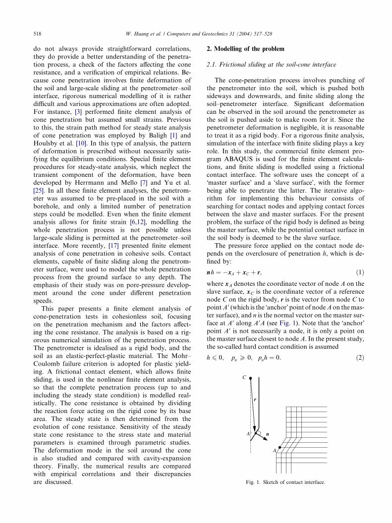
Fig. 1. Sketch of contact interface.

518 W. Huang et al. / Computers and Geotechnics 31 (2004) 517–528

do not always provide straightforward correlations,

they do provide a better understanding of the penetra-

tion process, a check of the factors affecting the cone

resistance, and a verification of empirical relations. Be-

cause cone penetration involves finite deformation of

the soil and large-scale sliding at the penetrometer–soilinterface, rigorous numerical modelling of it is rather

difficult and various approximations are often adopted.

For instance, [3] performed finite element analysis of

cone penetration but assumed small strains. Previous

to this, the strain path method for steady state analysis

of cone penetration was employed by Baligh [1] and

Houlsby et al. [10]. In this type of analysis, the pattern

of deformation is prescribed without necessarily satis-fying the equilibrium conditions. Special finite element

procedures for steady-state analysis, which neglect the

transient component of the deformation, have been

developed by Herrmann and Mello [7] and Yu et al.

[25]. In all these finite element analyses, the penetrom-

eter was assumed to be pre-placed in the soil with a

borehole, and only a limited number of penetration

steps could be modelled. Even when the finite elementanalysis allows for finite strain [6,12], modelling the

whole penetration process is not possible unless

large-scale sliding is permitted at the penetrometer–soil

interface. More recently, [17] presented finite element

analysis of cone penetration in cohesive soils. Contact

elements, capable of finite sliding along the penetrom-

eter surface, were used to model the whole penetration

process from the ground surface to any depth. Theemphasis of their study was on pore-pressure develop-

ment around the cone under different penetration

speeds.

This paper presents a finite element analysis of

cone-penetration tests in cohesionless soil, focusing

on the penetration mechanism and the factors affect-

ing the cone resistance. The analysis is based on a rig-

orous numerical simulation of the penetration process.The penetrometer is idealised as a rigid body, and the

soil as an elastic-perfect-plastic material. The Mohr–

Coulomb failure criterion is adopted for plastic yield-

ing. A frictional contact element, which allows finite

sliding, is used in the nonlinear finite element analysis,

so that the complete penetration process (up to and

including the steady state condition) is modelled real-

istically. The cone resistance is obtained by dividingthe reaction force acting on the rigid cone by its base

area. The steady state is then determined from the

evolution of cone resistance. Sensitivity of the steady

state cone resistance to the stress state and material

parameters is examined through parametric studies.

The deformation mode in the soil around the cone

is also studied and compared with cavity-expansion

theory. Finally, the numerical results are comparedwith empirical correlations and their discrepancies

are discussed.

2. Modelling of the problem

2.1. Frictional sliding at the soil-cone interface

The cone-penetration process involves punching of

the penetrometer into the soil, which is pushed bothsideways and downwards, and finite sliding along the

soil–penetrometer interface. Significant deformation

can be observed in the soil around the penetrometer as

the soil is pushed aside to make room for it. Since the

penetrometer deformation is negligible, it is reasonable

to treat it as a rigid body. For a rigorous finite analysis,

simulation of the interface with finite sliding plays a key

role. In this study, the commercial finite element pro-gram ABAQUS is used for the finite element calcula-

tions, and finite sliding is modelled using a frictional

contact interface. The software uses the concept of a

�master surface� and a �slave surface�, with the former

being able to penetrate the latter. The iterative algo-

rithm for implementing this behaviour consists of

searching for contact nodes and applying contact forces

between the slave and master surfaces. For the presentproblem, the surface of the rigid body is defined as being

the master surface, while the potential contact surface in

the soil body is deemed to be the slave surface.

The pressure force applied on the contact node de-

pends on the overclosure of penetration h, which is de-

fined by:

nh ¼ �xA þ xC þ r; ð1Þwhere xA denotes the coordinate vector of node A on the

slave surface, xC is the coordinate vector of a reference

node C on the rigid body, r is the vector from node C to

pointA 0 (which is the �anchor� point of nodeAon themas-

ter surface), and n is the normal vector on the master sur-

face at A 0 along A 0A (see Fig. 1). Note that the �anchor�point A 0 is not necessarily a node, it is only a point onthe master surface closest to nodeA. In the present study,

the so-called hard contact condition is assumed

h 6 0; pn P 0; pnh ¼ 0: ð2Þ

0p

smoo

th

W. Huang et al. / Computers and Geotechnics 31 (2004) 517–528 519

Herein, pn represents the contact pressure. Node A on

the slave surface is considered to be in contact with the

master surface only when h = 0 & pn > 0 . The contact

constraint is enforced with a Lagrangian multiplier,

which represents the contact pressure in a mixed

formulation [8].Sliding can occur if a node on the slave surface is in

contact with the master surface. In this case, a critical

shear stress can be calculated, based on the friction

law scrit = pn Æ tan /sc, where /sc denotes the frictional

angle on the penetrometer–soil interface. A contact node

is in a ‘‘sticky’’ state as long as the actual shear stress s isless than scrit, and an elastic response is assumed. Other-

wise, the contact node undergoes sliding, which is a per-fectly-plastic response.

2.2. Modelling of soil behaviour

A large number of constitutive models exist for differ-

ent soils. To capture as many aspects of soil behaviour

as possible, some of these are very sophisticated and in-

volve lots of parameters. However, in engineering prac-tice, simple models are often sufficient as only the key

features of soil behaviour are of importance. In this

study, a simple elastic-perfect-plastic model with the

Mohr–Coulomb yield criterion is used to describe the

behaviour of a cohesionless soil. The elastic deformation

is described by the elastic modulus E (or the shear mod-

ulus G) and the Poisson�s ratio t, while the plastic defor-mation is characterized by the friction angle /, thedilation angle w, and the cohesion c (c � 0 for a cohe-

sionless soil). A non-associated flow rule is used to sim-

ulate the dilatant behaviour of the soil.

A real cohesionless soil often exhibits density-depend-

ent behaviour. In response to large shear deformation,

the mobilized friction angle tends to a stationary value

(usually denoted by /c) which is known as the critical

friction angle. Peak strengths followed by softening areobserved only in initially dense sands. The present elas-

tic perfectly-plastic soil model has the soil friction and

dilation angles as two independent parameters. The crit-

ical state value is taken for the friction angle (/ = /c),

with the density effect being reflected by the dilation an-

gle. For the case where the peak friction angle is consid-

ered, it may be related to the dilation angle w through

Bolton�s relation [2]

/p ¼ /c þ 0:8w: ð3Þ

1 m

rough

Fig. 2. Finite element mesh for analysis.

2.3. Displacement finite element analysis

Displacement finite element analyses are performed

with geometric nonlinearity being taken into account.

Cauchy stress and the symmetric part of the velocity

gradient (also known as the stretching tensor) are used

to define the stress and strain rate in the deforming soil.

Equilibrium is checked on the current configuration and

a standard Newton iteration procedure is applied to

solve the governing nonlinear system of equations.

Cohesionless sandy soils, with a relatively large per-

meability, are considered so that any excess pore pres-

sure developed during the penetration process can beneglected, and a fully drained condition is assumed.

In the numerical calculations, a standard penetrome-

ter geometry is used — that is, a penetrometer with a

shaft diameter of dc = 35.7 mm and a tip angle of

a = 60�. The soil domain is modelled by an axi-symmetric

mesh of 1 m radius (about 56 times that of the cone

radius) and 2 m depth, with 1600 8-noded biquadratic

elements (Fig. 2). The grid is so designed that the ele-ments potentially in contact with the cone have a size of

about one-third of the cone radius. The element size is in-

creased both horizontally and vertically from the pene-

trometer to control the total number of equations to be

solved. Test runs have shown that further refinement of

the mesh has no significant influence on the numerical

results.

Due to the large number of degrees of freedom in themesh, as well as the material and geometric nonlineari-

ties, simulation of a very deep penetrometer would re-

quire a huge amount of CPU time. This problem is

overcome by applying a vertical overburden pressure

p0 on the top boundary of the mesh to represent the

stress state at a specific depth. The nodes on the bottom

boundary are fixed, while the nodes on the right-hand

side are allowed to move vertically. The left boundary

520 W. Huang et al. / Computers and Geotechnics 31 (2004) 517–528

is the axis of symmetry. The initial stress state is charac-

terized by the overburden pressure p0 and the lateral

earth pressure coefficient K0 only. The self-weight of

the soil in the computation domain is not included, so

as to give better control of the vertical stress (which is

specified and models the effect of gravity). This omissionof the self-weight does not change the penetration mech-

anism and, therefore, will not significantly affect the nor-

malized cone resistance. Indeed, this approach simplifies

the treatment of the calculated cone factors and can lead

to a better estimation of the so-called steady state (which

is characterized by a constant cone resistance instead of

a linearly increasing cone resistance). Initially, the cone

is located on the top boundary and the penetration proc-ess is simulated by applying a vertical displacement to it.

In all numerical calculations, the soil cohesion c is set to

zero and Poisson�s ratio is fixed at 0.3. Parametric stud-

ies are performed to investigate the influence of the pres-

sure level p0, the shear modulus G, the soil internal

friction angle /, and the dilation angle w.

3. Evolution of cone resistance and interfacial friction

The reaction force during penetration, obtained from

the numerical calculations, represents the total pushing

force acting on the penetrometer. This total pushing

force, denoted by Ft, is equal to the sum of the resistance

force on the cone, Fc, and the friction force on the shaft,

Fs, i.e.

F t ¼ F c þ F s: ð4ÞIn Fig. 3, numerical results are shown for the evolu-

tion of the total pushing force Ft obtained for different

penetrometer–soil interface friction angles /sc. Two

phases can be observed in these evolution curves. The

first phase corresponds to a strongly nonlinear variationin Ft as the depth of penetration z increases. The inter-

facial friction angle /sc has only a minor influence dur-

ing this transient phase. The second phase starts at a

critical penetration depth zc, and is characterised by a

Fig. 3. Evolution of total reaction force acting on the rigid body for

various interfacial frictions (/ = 30�, w = 10�, G/p0 = 100, p0 = 10 kPa,

K0 = 1.0).

nearly linear increase in the total pushing force with z.

The greater the interfacial friction, the faster the increase

in the total pushing force. It is notable that the total

pushing force Ft remains almost constant for /sc = 0.

Therefore, the second phase corresponds to the so-called

steady state. Small numerical oscillations are observedin the evolution curves for Ft. The critical depth zc was

found to be related to the size of the plastic zone in

the soil which, in turn, depends on the stress state and

the soil properties.

Penetrometers are usually designed to allow the cone

resistance, and sometimes the sleeve friction, to be meas-

ured. The former is the most important quantity for

engineering design, and is defined as

qc ¼ 4F c=pd2c ; ð5Þ

where dc is the shaft diameter of the cone. As only Ft in

Eq. (2) can be obtained directly from finite element cal-

culations, it is necessary to identify the cone resistanceforce Fc separately. To achieve this end, the interfacial

friction /sc was set to zero in the finite element calcula-

tions. Thus the obtained total reaction force is the same

as the resistance force on the cone, i.e. F cj/sc¼0 ¼ F tj/sc¼0.

Note that, for a non-zero interface friction angle, the

interfacial friction on the cone tip makes a contribution

to the actual cone resistance. By neglecting it, only the

nominal cone resistance �qc ¼ qcj/sc¼0 is obtained throughEq. (5).

To account for the contribution of interfacial friction

to the total cone resistance, the nominal cone resistance

can be multiplied by a tip friction factor, g, so that

qc ¼ g�qc: ð6ÞThe tip friction factor g is estimated analytically by

considering simple equilibrium of the cone (refer to

Fig. 4). With the presence of interface friction, the total

cone resistance force can be expressed as

qcAc ¼ZA0c

pnðsinða=2Þ þ cosða=2Þ tan/scÞ dA0c

¼ ðsinða=2Þ þ cosða=2Þ tan/scÞZA0c

pn dA0c;

where A0c represents the tip area and a the tip angle of the

cone. By setting /sc = 0 we have �qcAc ¼ sinða=2ÞRA0cpn dA

0c. Under finite strain conditions, changing the

Fig. 4. Illustration of contribution of the interface friction to the cone

resistance.

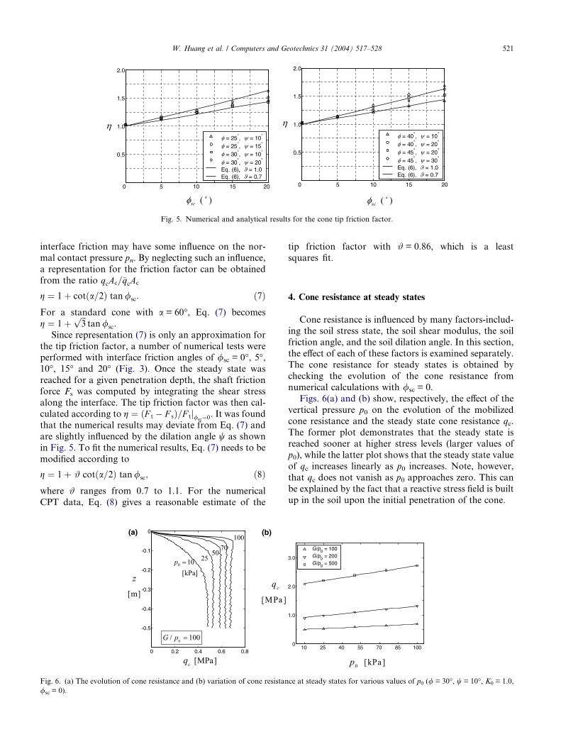
Fig. 5. Numerical and analytical results for the cone tip friction factor.

W. Huang et al. / Computers and Geotechnics 31 (2004) 517–528 521

interface friction may have some influence on the nor-

mal contact pressure pn. By neglecting such an influence,

a representation for the friction factor can be obtained

from the ratio qcAc=�qcAc

g ¼ 1þ cotða=2Þ tan/sc: ð7ÞFor a standard cone with a = 60�, Eq. (7) becomes

g ¼ 1þffiffiffi3

ptan/sc.

Since representation (7) is only an approximation for

the tip friction factor, a number of numerical tests were

performed with interface friction angles of /sc = 0�, 5�,10�, 15� and 20� (Fig. 3). Once the steady state was

reached for a given penetration depth, the shaft friction

force Fs was computed by integrating the shear stressalong the interface. The tip friction factor was then cal-

culated according to g ¼ ðF t � F sÞ=F tj/sc¼0. It was found

that the numerical results may deviate from Eq. (7) and

are slightly influenced by the dilation angle w as shown

in Fig. 5. To fit the numerical results, Eq. (7) needs to be

modified according to

g ¼ 1þ # cotða=2Þ tan/sc; ð8Þwhere # ranges from 0.7 to 1.1. For the numerical

CPT data, Eq. (8) gives a reasonable estimate of the

(a) (b)

Fig. 6. (a) The evolution of cone resistance and (b) variation of cone resistan

/sc = 0).

tip friction factor with # = 0.86, which is a least

squares fit.

4. Cone resistance at steady states

Cone resistance is influenced by many factors-includ-ing the soil stress state, the soil shear modulus, the soil

friction angle, and the soil dilation angle. In this section,

the effect of each of these factors is examined separately.

The cone resistance for steady states is obtained by

checking the evolution of the cone resistance from

numerical calculations with /sc = 0.

Figs. 6(a) and (b) show, respectively, the effect of the

vertical pressure p0 on the evolution of the mobilizedcone resistance and the steady state cone resistance qc.

The former plot demonstrates that the steady state is

reached sooner at higher stress levels (larger values of

p0), while the latter plot shows that the steady state value

of qc increases linearly as p0 increases. Note, however,

that qc does not vanish as p0 approaches zero. This can

be explained by the fact that a reactive stress field is built

up in the soil upon the initial penetration of the cone.

ce at steady states for various values of p0 (/ = 30�, w = 10�, K0 = 1.0,

(a) (b)

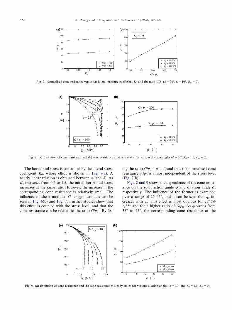
Fig. 7. Normalised cone resistance versus (a) lateral pressure coefficient K0 and (b) ratio G/p0 (/ = 30�, w = 10�, /sc = 0).

(a) (b)

Fig. 8. (a) Evolution of cone resistance and (b) cone resistance at steady states for various friction angles (w = 10�,K0 = 1.0, /sc = 0).

522 W. Huang et al. / Computers and Geotechnics 31 (2004) 517–528

The horizontal stress is controlled by the lateral stress

coefficient K0, whose effect is shown in Fig. 7(a). A

nearly linear relation is obtained between qc and K0 As

K0 increases from 0.5 to 1.5, the initial horizontal stress

increases at the same rate. However, the increase in the

corresponding cone resistance is relatively small. The

influence of shear modulus G is significant, as can be

seen in Fig. 6(b) and Fig. 7. Further studies show thatthis effect is coupled with the stress level, and that the

cone resistance can be related to the ratio G/p0 . By fix-

(a) (b)

Fig. 9. (a) Evolution of cone resistance and (b) cone resistance at steady

ing the ratio G/p0 it was found that the normalised cone

resistance qc/p0 is almost independent of the stress level

(Fig. 7(b)).

Figs. 8 and 9 shows the dependence of the cone resist-

ance on the soil friction angle / and dilation angle w,respectively. The influence of the former is examined

over a range of 25–45�, and it can be seen that qc in-

creases with /. This effect is most obvious for 25�6/635� and for a higher ratio of G/p0. As / varies from

35� to 45�, the corresponding cone resistance at the

states for various dilation angles (/ = 30� and K0 = 1.0, /sc = 0).

Fig. 11. Plots of the plastic zone at different depths of penetration: (a)

2.5 dc; (b)5.1 dc; (c) 10.2 dc; (d) 14.0 dc, with dc and being the cone

W. Huang et al. / Computers and Geotechnics 31 (2004) 517–528 523

steady state varies only slightly, even though the tran-

sient responses are rather different (Fig. 8(a)). This could

be related to the fact that cone penetration is basically a

deformation controlled test. As the total deformation is

fixed, an increase in the yield limit is accompanied by a

decrease in the size of the plastic zone and only a slightincrease in the cone resistance. In contrast, varying the

angle of dilation has a pronounced effect on the cone re-

sponse. Increasing w leads to an obvious increase in

cone resistance, with deeper penetration being needed

to reach the steady state. This result stems from dilation

in the plastic zone, which increases the mean pressure

and hence the cone resistance.

diameter (G/p0 = 100, / = 30�, w = 10�).

Fig. 12. Plots of the steady state plastic zone for: (a) p0 = 10 kPa; (b)

p0 = 25 kPa; (c) p0 = 50 kPa; (d) p0 = 100 kPa (G = 2000 kPa, / = 30�,w = 10�).

5. Soil deformation and plastic zone

Penetration of a cone into the ground involves push-

ing the surrounding soil downwards and sideways. The

process can be clearly understood by viewing the de-

formed mesh and displacement field in the soil around

the penetrometer, as shown in Fig. 10. It can be seenthat the soil particles on the axis of symmetry move only

vertically downwards, whereas soil particles in contact

with the cone surface are pushed sideways as well. From

the cone tip to the shaft, the horizontal displacement of

soil particles increases, with the maximum horizontal

displacement being observed at the edge of the cone.

This maximum displacement is controlled by the diame-

ter of the penetrometer shaft. If only the horizontal dis-placement is considered, the penetration process

resembles a cylindrical cavity expansion to a limited ra-

dius. The vertical displacement component exists due to

the inclined surface of the cone and the interface fric-

tion. By looking at a plot of the plastic zone around

the penetrometer (Fig. 11), we can see that its shape dif-

fers from those predicted by cylindrical or spherical cav-

ity expansion theory [20,16]. These plots indicate thatthe plastic zone enlarges and moves downwards as the

Fig. 10. (a) Deformed mesh and (b) displaceme

cone is inserted in the soil. It ceases to grow once the

cone reaches the steady state penetration depth. This

depth is reached earlier for cases where the size of the

stable plastic zone is smaller. Fig. 12 shows plots of

the steady state plastic zone for various values of initial

pressure. It can be seen that the size of the plastic zone

decreases as the initial pressure increases.

The shape of the moving plastic zone around the conetip resembles that of half an ellipse, with the longer axis

nt field around the cone at a steady state.

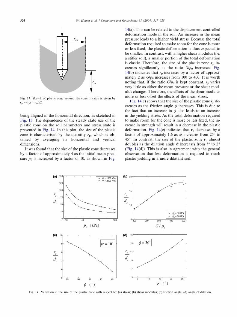
Fig. 13. Sketch of plastic zone around the cone; its size is given by

rp = (rph + rpv)/2.

524 W. Huang et al. / Computers and Geotechnics 31 (2004) 517–528

being aligned in the horizontal direction, as sketched in

Fig. 13. The dependence of the steady state size of the

plastic zone on the soil parameters and stress state is

presented in Fig. 14. In this plot, the size of the plastic

zone is characterised by the quantity rp, which is ob-

tained by averaging its horizontal and verticaldimensions.

It was found that the size of the plastic zone decreases

by a factor of approximately 4 as the initial mean pres-

sure p0 is increased by a factor of 10, as shown in Fig.

(a) (

((c)

Fig. 14. Variation in the size of the plastic zone with respect to: (a) s

14(a). This can be related to the displacement-controlled

deformation mode in the soil. An increase in the mean

pressure leads to a higher yield stress. Because the total

deformation required to make room for the cone is more

or less fixed, the plastic deformation is thus expected to

be smaller. In contrast, with a higher shear modulus (i.e.a stiffer soil), a smaller portion of the total deformation

is elastic. Therefore, the size of the plastic zone rp in-

creases significantly as the ratio G/p0 increases. Fig.

14(b) indicates that rp increases by a factor of approxi-

mately 2 as G/p0 increases from 100 to 400. It is worth

noting that, if the ratio G/p0 is kept constant, rp varies

very little as either the mean pressure or the shear mod-

ulus changes. Therefore, the effects of the shear modulusmore or less offset the effects of the mean stress.

Fig. 14(c) shows that the size of the plastic zone rp de-creases as the friction angle / increases. This is due to

the fact that an increase in / also leads to an increase

in the yielding stress. As the total deformation required

to make room for the cone is more or less fixed, the in-

crease in strength will result in a decrease in the plastic

deformation. Fig. 14(c) indicates that rp decreases by afactor of approximately 1.6 as / increases from 25� to

45�. In contrast, the size of the plastic zone rp almost

doubles as the dilation angle w increases from 5� to 25

(Fig. 14(d)). This is also in agreement with the general

observation that less deformation is required to reach

plastic yielding in a more dilatant soil.

b)

d)

tress; (b) shear modulus; (c) friction angle; (d) angle of dilation.

W. Huang et al. / Computers and Geotechnics 31 (2004) 517–528 525

6. Comparison with empirical correlations

In the parametric study presented above, only one

soil parameter is varied each time. This is rarely true

for real soils. Therefore, the correlations between the

cone resistance and each of the soil parameters mightnot apply in practice. However, numerical studies can

provide a proper assessment of existing empirical corre-

lations. Most of these correlations fall into two catego-

ries: those which are based on the solution of bearing-

capacity problems, and those which are based on the

theory of cavity expansion.

Empirical correlations of the first category are usually

expressed in simple forms that relate the friction anglewith cone resistance – as, for instance, in the correlation

proposed by Robertson and Campanella [15], which

reads

qc=p0 ¼ C2 exp½C1 tan/� ð9Þ

with C1 = 6.820 and C2 = 0.266. In bearing-capacity

analysis, only the limit equilibrium state of collapse isconsidered, with the soil compressibility and soil defor-

mation being neglected. However, cone penetration is

more of a displacement-controlled steady deformation

process than a limit equilibrium problem. The compres-

sibility of the soil has a strong influence on the cone

resistance, which is not reflected by this type of correla-

(a)

(c)

(b

Fig. 15. Comparison of correlation (9) (solid curves) with numerical resul

w = 10�; (b) various friction angles with associate flow; (c) various peak fric

tion. Therefore the applicability of this type of correla-

tion is limited.

The comparison between the finite element results

(dashed curves) and the prediction of Eq. (9) (solid

curves) is presented in Fig. 15. In these plots the cone

resistances from finite element calculations have beenadjusted by multiplying the tip friction factor g given

in Eq. (8) for /sc = 10� . Significant differences betweenthe numerical and empirical correlations can be seen.

Since the dilation angle is not explicitly included in

Eq. (9), comparison is made for a fixed dilation angle

w = 10� (Fig. 15(a)), for an associated flow rule with

w = / (Fig. 15(b)), and by setting / = /p in Eq. (9),

which is related to the variation of dilation angle viaBolton�s relation (3) with /c = 30�.

Empirical correlations of the second category are of-

ten in a more complicated form, as they depend on solu-

tions to cavity expansion problems. In fact, closed form

analytical solutions are not always available, particu-

larly for the Mohr–Coulomb yield criterion with a

non-associated flow rule. Vesic [19] presented a simpli-

fied solution for cavity expansion in infinite Mohr–Cou-lomb soil. Based on this solution, he proposed a

correlation for cone resistance, which reads [20]:

qcp0

¼ 1þ 2K0

3� sin/exp½ðp=2� /Þ tan /� tan2ðp=4þ /=2Þ Inrr;

ð10Þ

)

ts (dashed curves) for: (a) various friction angles with dilation angle

tion and dilatancy angles given through Bolton�s relation (3).

(a) (b)

(c)

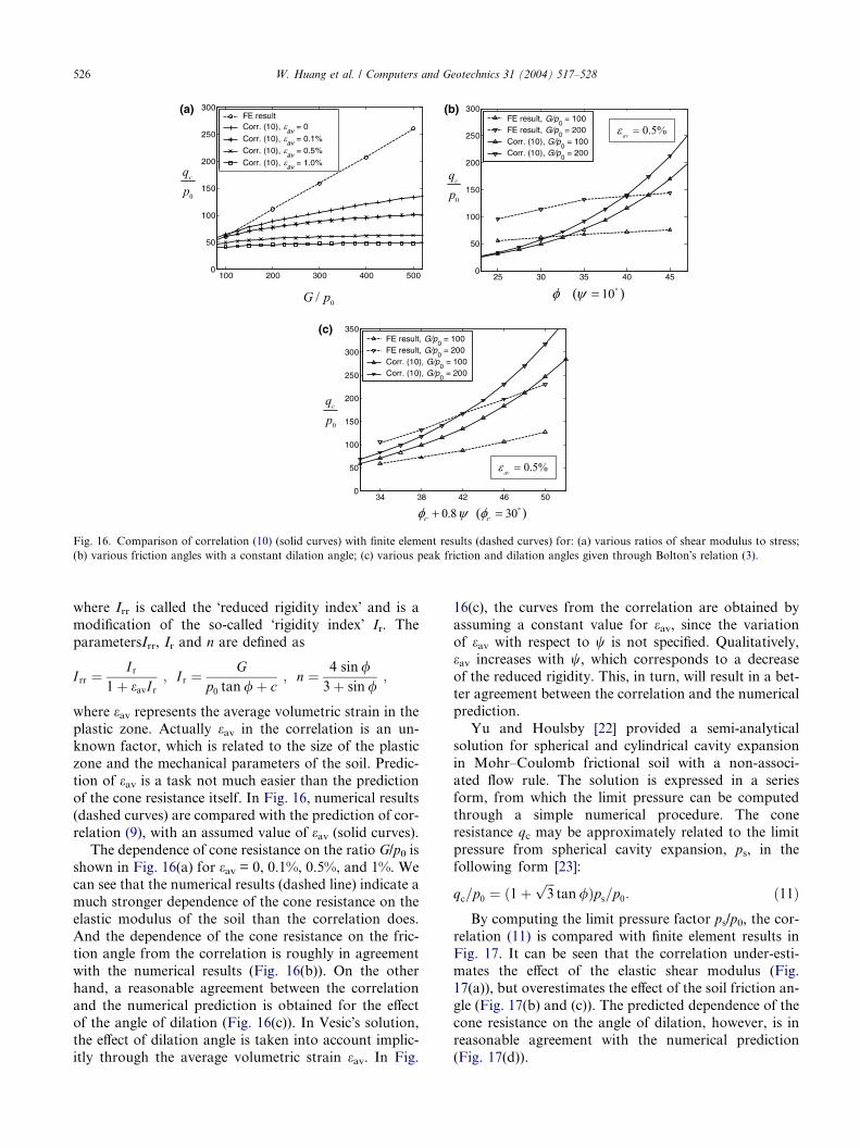
Fig. 16. Comparison of correlation (10) (solid curves) with finite element results (dashed curves) for: (a) various ratios of shear modulus to stress;

(b) various friction angles with a constant dilation angle; (c) various peak friction and dilation angles given through Bolton�s relation (3).

526 W. Huang et al. / Computers and Geotechnics 31 (2004) 517–528

where Irr is called the �reduced rigidity index� and is a

modification of the so-called �rigidity index� Ir. The

parametersIrr, Ir and n are defined as

I rr ¼I r

1þ eavI r; I r ¼

Gp0 tan/þ c

; n ¼ 4 sin/3þ sin/

;

where eav represents the average volumetric strain in the

plastic zone. Actually eav in the correlation is an un-known factor, which is related to the size of the plastic

zone and the mechanical parameters of the soil. Predic-

tion of eav is a task not much easier than the prediction

of the cone resistance itself. In Fig. 16, numerical results

(dashed curves) are compared with the prediction of cor-

relation (9), with an assumed value of eav (solid curves).

The dependence of cone resistance on the ratio G/p0 is

shown in Fig. 16(a) for eav = 0, 0.1%, 0.5%, and 1%. Wecan see that the numerical results (dashed line) indicate a

much stronger dependence of the cone resistance on the

elastic modulus of the soil than the correlation does.

And the dependence of the cone resistance on the fric-

tion angle from the correlation is roughly in agreement

with the numerical results (Fig. 16(b)). On the other

hand, a reasonable agreement between the correlation

and the numerical prediction is obtained for the effectof the angle of dilation (Fig. 16(c)). In Vesic�s solution,the effect of dilation angle is taken into account implic-

itly through the average volumetric strain eav. In Fig.

16(c), the curves from the correlation are obtained by

assuming a constant value for eav, since the variation

of eav with respect to w is not specified. Qualitatively,eav increases with w, which corresponds to a decrease

of the reduced rigidity. This, in turn, will result in a bet-

ter agreement between the correlation and the numerical

prediction.

Yu and Houlsby [22] provided a semi-analytical

solution for spherical and cylindrical cavity expansion

in Mohr–Coulomb frictional soil with a non-associ-

ated flow rule. The solution is expressed in a seriesform, from which the limit pressure can be computed

through a simple numerical procedure. The cone

resistance qc may be approximately related to the limit

pressure from spherical cavity expansion, ps, in the

following form [23]:

qc=p0 ¼ ð1þffiffiffi3

ptan/Þps=p0: ð11Þ

By computing the limit pressure factor ps/p0, the cor-

relation (11) is compared with finite element results in

Fig. 17. It can be seen that the correlation under-esti-mates the effect of the elastic shear modulus (Fig.

17(a)), but overestimates the effect of the soil friction an-

gle (Fig. 17(b) and (c)). The predicted dependence of the

cone resistance on the angle of dilation, however, is in

reasonable agreement with the numerical prediction

(Fig. 17(d)).

(a) (b)

(d)(c)

Fig. 17. Comparison of correlation (11) based on Yu and Houlsby solution (solid curves) with finite element results (dashed curves) for: (a) various

ratios of shear modulus to stress; (b) various friction angles with a constant dilation angle; (c) various friction angles with associated flow; (d) various

peak friction and dilation angles given through Bolton�s relation (3).

W. Huang et al. / Computers and Geotechnics 31 (2004) 517–528 527

Generally speaking, the cone-penetration process is

closer to being a cavity-expansion problem than to being

a bearing-capacity problem. If only the horizontal dis-

placement of the soil around the cone is considered,

the penetration process is similar to a cylindrical cavity

expansion. However, with consideration of the vertical

displacements in the soil around the cone and within

the plastic zone, the degree of similarity becomes un-clear. In addition, in cavity-expansion theory, the limit

pressure for cavity expansion is usually used for correla-

tion with the cone resistance. The limit pressure in a cav-

ity expansion corresponds to a state in which the

pressure does not change with further expansion of the

cavity, a state that can be approached asymptotically

with a very large expansion. In the cone-penetration

process, the soil particles around the cone might notreach such a large displacement. As the cone tip cuts

into the soil, and as sliding occurs at the interface, the

vertical displacements of the soil particles are limited.

The horizontal displacements of these particles are also

limited (they are controlled by the diameter of the pene-

trometer shaft). Consequently, the stress state in the soil

around the cone surface might not approach the limit

pressure, as assumed in cavity-expansion theory. Thefact that the size of the plastic zone decreases with

increasing friction angle also indicates that the limit

pressure is not approached in the cone-penetration proc-

ess. This fact explains why correlations based on cavity

expansion theory underestimate the effect of the elastic

modulus, but overestimate the effect of the friction an-

gle, on the cone resistance.

7. Conclusion

Simulating the process of cone penetration rigorously

depends on accurate modelling of both the soil and inter-face behaviour. By including finite deformation of the

soil and large scale sliding at the penetrometer–soil inter-

face, the complete penetration process, starting from the

ground surface, can be modelled. It has been shown that

steady states can be observed following a transient peri-

od of penetration. The penetration depth of the transient

phase is related to the steady state size of the plastic zone

developed around the cone and the shaft. The size of thiszone depends on the stress state and soil deformation

parameters, as well as strength parameters.

In a cone-penetration test, soil around the cone is

pushed downwards and outwards to accommodate the

penetrometer. The horizontal displacement of soil parti-

cles around the cone is controlled by the size of the pene-

trometer shaft, whereas the vertical displacement

depends on the elastic properties of the soil, the frictionat the conesoil interface, and the strength of the soil. The

true deformation pattern around a penetrating cone is

somewhat different from that assumed in bearing-capac-

ity theory or cavity-expansion theory. This is because

the soil around the cone or shaft does not necessarily

528 W. Huang et al. / Computers and Geotechnics 31 (2004) 517–528

approach the limit strength state. Parametric studies

show that the cone resistance is influenced more by

deformation properties (such as shear modulus and an-

gle of dilation) than by shear strength parameters (such

as the friction angle).

Comparatively, steady state penetration is more sim-ilar to a cavity expansion problem than a bearing capac-

ity problem. A preliminary comparison presented in this

paper suggests that a reasonable agreement has been ob-

tained between the numerical results and correlations

based on cavity expansion theory. It has also been found

that most empirical correlations tend to underestimate

the influence of elastic modulus and overestimate the

influence of the friction angle, particularly for compress-ible soils.

Although a more realistic penetration process is mod-

elled in this study, the current work has been focused on

the cone resistance and did not use the computed values

of sleeve friction. This is mainly because a homogeneous

soil is considered and an assumed interface friction is ap-

plied in the numerical analysis. In practice, sleeve fric-

tion is usually used for soil classification. For a furtherstudy, the effects of interface friction could be consid-

ered for varying roughnesses of the friction sleeve, to-

gether with the micropolar effects of soils. Further

work is also needed to investigate the effects of other soil

models with a more detailed comparison between the FE

solutions and experimental data. Other existing analyti-

cal/numerical methods for CPT analysis could also be

investigated.

References

[1] Baligh MM. Strain path method. ASCE J Soil Mech Found Div

1985;111(9):1108–36.

[2] Bolton MD. The strength and dilatancy of sands. Geotechnique

1986;36(1):65–78.

[3] De Borst R, Vermeer PA. Finite element analysis of static

penetration tests. Geotechnique 1984;34(2):199–210.

[4] De Simone P, Golia G. Theoretical analysis of the cone

penetration test in sands. In: Proceedings of the 1st International

Symposium on Penetration Testing, 1988; vol. 2. p. 729–35.

[5] Durgunoglu HT, Mitchell JK. Static penetration resistance of

soils. I-II. In: Proceedings of the ASCE Spec Conference on In

Situ Measurement of Soil Properties, 1975; vol. 1: p. 51–89.

[6] Gupta RC. Finite element analysis for deep cone penetration.

ASCE J Geotech Eng 1992;177(10):1610–30.

[7] Herrmann LR, Mello J. Investigation of an alternative finite

element procedure: a one-step, steady-state analysis. Report No.

CR 95.001, Dept. of Civil and Environmental Eng., University of

California at Davis, USA; 1994.

[8] Hibbitt, Karlsson, Sorensen, Inc., ABAQUS theory manual,

Version 6.2; 2001.

[9] Houlsby GT, Wroth CP. Determination of undrained strengths

by cone penetration tests. In: Proceedings of the 2nd European

Symposium on Penetration testing, 1982; vol. 2. p. 585–90.

[10] Houlsby GT, Wheeler AA, Norbury J. Analysis of undrained

cone penetration as a steady flow problem. In: Proceedings of the

5th International Conference on Numerical Methods in Geome-

chanics, 1985; vol. 4. p. 1767–73.

[11] Janbu N, Senneset K. Effective stress interpretation of in situ

static penetration tests. In: Proceedings of the 1st European

Symposium on Penetration Testing, 1974; vol. 2. p. 181–93.

[12] Kiousis PD, Voyiadjis GZ, Tumay MT. A large strain theory and

its application in the analysis of the cone penetration mechanism.

Int J Num Anal Meth, Geomech 1988;12:45–60.

[13] Ladanyi B, Johnson GH. Behaviour of circular footings and plate

anchors embedded in permafrost. Can Geotech J 1974;11:531–53.

[14] Lunne T, Robertson PK, Powell JJM. Cone penetration testing in

geotechnical practice. London: Blackie; 1997.

[15] Robertson PK, Campanella RG. Interpretation of cone penetra-

tion tests. I: Sand. Can Geotech J 1983;20:718–33.

[16] Salgado R, Mitchell JK, Jamiolkowski M. Cavity expansion and

penetration resistance in sand. ASCE J Geotech Geoenv Eng

1997;123(4):344–54.

[17] Sheng, D, Axelsson, K, Magnusson, O. Stress and strain fields

around a penetrating cone. In: Proceedings of the 6th Interna-

tional Symposium on Numerical Models in Geomechanics –

NUMOG-VI, July 1997, Montreal, Canada, Balkema, Rotter-

dam, 1997; p. 456–65.

[18] Van den Berg, P., 1994. Analysis of soil penetration. Ph.D. thesis,

Delft University, The Netherland.

[19] Vesic AS. Expansion of cavities in infinite soil mass. ASCE J soil

Mech Found Div 1972;98:265–90.

[20] Vesic, A.S.. Design of pile foundations. National Cooperation

Highway Research Program Report No. 42, Transaction

Research Board, Washington, DC; 1977.

[21] Wroth CP. The interpretation of in situ soil test. 24th Rankine

Lecture. Geotechnique 1984;34(4):449–89.

[22] Yu HS, Houlsby GT. Finite cavity expansion in dilatant soils:

loading analysis. Geotechnique 1991;41(2):173–83.

[23] Yu HS, Schnaid F, Collins IF. Analysis of cone pressuremeter

tests in sands. J Geotech Eng ASCE 1996;122(8):623–32.

[24] Yu HS, Mitchell JK. Analysis of cone resistance: a review of

methods. J Geotech Geoenv Eng ASCE 1998;124(2):140–9.

[25] Yu HS, Herrmann LR, Boulanger RW. Analysis of steady cone

penetration in clay. J Geotech Geoenv Eng ASCE 2000;126(7):

594–605.