
emagtm
246
-
Upload
ganesan-subramanian -
Category
Documents
-
view
261 -
download
1
Transcript of emagtm

8/12/2019 emagtm
http://slidepdf.com/reader/full/emagtm 1/246

8/12/2019 emagtm
http://slidepdf.com/reader/full/emagtm 2/246
8/12/2019 emagtm
http://slidepdf.com/reader/full/emagtm 3/246
NISA/EMAG Training Manual Table of Contents
i
Table of Contents
Chapter 1 Introduction.................................................................................................... 1-1
Chapter 2 Installation Instructions ................................................................................. 2-1
Chapter 3 DISPLAY III – How it Works ....................................................................... 3-1
Chapter 4 DISPLAY III – Basic Options for Geometric Modeling ............................... 4-1
Chapter 5 DISPLAY III – Basic Options for Finite Element Modeling ........................ 5-1
Chapter 6 DISPLAY III – Miscellaneous Options ......................................................... 6-1
Chapter 7 Low Frequency Analysis ............................................................................... 7-1
Chapter 8 Modeling Session 1 ....................................................................................... 8-1
Chapter 9 Modeling Session 2 ....................................................................................... 9-1
Chapter 10 Modeling Session 3 ..................................................................................... 10-1
Chapter 11 Modeling Session 4 ..................................................................................... 11-1
Chapter 12 Modeling Session 5 ..................................................................................... 12-1
Chapter 13 Modeling Session 6 ..................................................................................... 13-1
Chapter 14 Modeling Session 7 ..................................................................................... 14-1
Chapter 15 Modeling Session 8 ..................................................................................... 15-1
Chapter 16 Modeling Session 9 ..................................................................................... 16-1

8/12/2019 emagtm
http://slidepdf.com/reader/full/emagtm 4/246

8/12/2019 emagtm
http://slidepdf.com/reader/full/emagtm 5/246
NISA/EMAG Training Manual Introduction
1-1
CHAPTER 1
INTRODUCTION
NISA/EMAG (Numerically Integrated elements for System Analysis, forELECTROMAGNETIC problems) is a general purpose finite element based computationalelectromagnetic code developed and maintained by EMRC to analyze electromagnetic field problems encountered in Electrical Engineering. NISA/EMAG is coupled with NISA/HEATfor analyzing coupled electrical and heat problems. Electromagnetic field analysis forarbitrary shaped domains with various possible boundary conditions require numerical toolssince the Maxwell’s equations and the equation of continuity must be satisfied along witharbitrarily specified boundary conditions. The material encountered can in general beanisotropic and non-linear. NISA/EMAG incorporates such tools into an integrated package.2D, axisymmetric and 3D arbitrary geometry can be simulated for all electromagnetic field problems. This program is comprised of two modules: Low frequency and High frequency.
The Low frequency module of NISA/EMAG handles electrical charges flowing or varyingat low frequency. For this the effect of Displacement current can be neglected. Itsapplications span a wide range of Electrical industries manufacturing Transformers,Electrical machines, Capacitors, Inductors, Resistors, Solenoids, Electrostatic devices,Biomedical equipments, High voltage equipments, Integrated circuit Technology, Electricalfurnaces and ovens, Electro-chemical cells etc.
The High frequency module of NISA/EMAG analyses high frequency devices ( Microwave,Millimeter and Optic frequency range) viz. Transmission lines, waveguides, waveguidediscontinuities, Integrated circuits, Couplers, Isolators, Circulators, Resonators, Antennasand scattering surfaces.
A brief overview of NISA/EMAG capabilities is given below.
Pre-processing
NISA/EMAG directly interfaces with the pre-processing module of the DISPLAY program;a 3D interactive color graphic program with extensive modeling capabilities for finiteelement model generation and problem definition. Highlights of the capabilities are:
• Both command and menu driven modes, with on-line help.
• 3-D geometric modeling including points, lines, arcs, curves, surfaces and solids as well
as surface intersections.
• Geometric transformations including translation, rotation, scaling, mirror imaging anddragging a curve along an arbitrary 3-D path.
• 3-D interactive finite element mesh generation including automatic node and elementgeneration.
• Mesh grading with uniform or non-uniform spacing.

8/12/2019 emagtm
http://slidepdf.com/reader/full/emagtm 6/246
Introduction NISA/EMAG Training Manual
1-2
• Merging separate models into larger one.
• Definition of element attributes including material and geometric properties.
• Specification of boundary conditions.
• Extensive model editing capabilities.
• Extensive plotting options including boundary line, hidden line removal and shrinkelement plots for selected elements or regions.
• Color shading and light effects.
• Model checking including calculation of element areas, volumes, normals and distortionindex.
•
Complete NISA/EMAG data deck generation.
Input data structure
• Simple modular input data structure and easy to use free format.
• Descriptive data group identification names reflecting the function of each data group.For example, electromagnetic material properties are entered in *MATEMAG datagroup.
• The data deck consists of three data blocks : The executive commands specifying theoverall control parameters in simple alphanumeric format, the model data block
describing the model characteristics and finally the analysis data block specifying thecurrent density, charge density, magnetic coercivity, boundary conditions and outputoptions.
• Data groups may appear in any order within each data block, with very few exceptions.
• Annotation echo of the input data.
• Extensive data checking and self-explanatory diagnostic messages.
Analysis Capability
Low frequency
The Low frequency module of NISA/EMAG is coupled with NISA/HEAT. Majorcapabilities of the Low frequency module of NISA/EMAG are categorized as follows:
• Main Analysis Types! Electric Field Analysis
8/12/2019 emagtm
http://slidepdf.com/reader/full/emagtm 7/246
NISA/EMAG Training Manual Introduction
1-3
! Magnetic Field Analysis
• Sub-Analysis Types! Electric Field Analysis
♦ Electrostatic Analysis♦ Steady State current flow
! Magnetic Field Analysis♦ Magnetostatic Analysis
# Using Magnetic vector potential# Using Magnetic scalar potential
♦ Magnetodynamic Analysis# For sinusoidal time variation using Magnetic vector potential# For arbitrary time variation using Magnetic vector potential
• Problem Dimensions! 2D!
Axisymmetric! 3D
• Types of Boundary Conditions! Dirichlet Boundary Conditions
# Electrostatic scalar Potential# Magnetic scalar and Vector Potential
! Neumann Boundary Conditions# Electric Flux Density# Magnetic Flux Density
! Source Boundary Condition# Electric Current Density# Electric Charge Density# Magnetic Coercivity# Current Density
• Non-linear Material specification! Magnetic material Properties
# B – H curve in Tabular form
• Property specification! Temperature Dependent Material Properties
♦ Permeability♦ Permittivity♦ Conductivity
# Tabular# Polynomial
! Orthotropic Properties

8/12/2019 emagtm
http://slidepdf.com/reader/full/emagtm 8/246
Introduction NISA/EMAG Training Manual
1-4
# Conductivity# Permeability# Permitivity
Major capabilities of the Heat module of NISA/HEAT are categorized as follows:
• Types of heat transfer analysis! Conduction Heat Transfer Analysis! Forced Convection Analysis! Natural Convection Analysis! Mixed Convection Analysis! Phase Change Analysis! Surface Radiation Analysis
• Types of Boundary Conditions! Dirichlet Boundary Conditions
# Temperature
! Neumann Boundary Conditions# Heat Flux
! Surface Convection Boundary Condition
! Radiative Boundary Condition
! Surface Radiation# Symmetry Plane# Outlets# Surfaces
! Time-dependent Boundary Condition# Temperature# Element Heat Generation# Surrounding/ambient temperature# Heat Flux
! Boundary Conditions in Local Coordinate Systems# Convection Heat Transfer Coefficient# Emissivity# Element heat generation# Heat Flux
! Nodal Heat Source and Element Generation
• Property specification! Temperature Dependent Material Properties
# Tabular# Polynomial

8/12/2019 emagtm
http://slidepdf.com/reader/full/emagtm 9/246
NISA/EMAG Training Manual Introduction
1-5
! Orthotropic Properties# Conductivity
High Frequency
Major capabilities of the High frequency module of NISA/EMAG are categorized as
follows:
• Type of analysis! Quasi-Static Analysis! Full Wave Analysis for Guided Waves! Full Wave Analysis for Resonant Cavities! Wave Scattering
• Problem Dimensions! 2D! Axisymmetric! 3D
• Type of boundary conditions# Electric Field Intensity# Magnetic Field Intensity# Absorbing Boundary conditions
Output Features
Various combinations of results at each node can be chosen to meet individual interest. Theformat of these results is consistent with the input format of DISPLAY III. The results
depend on the type of Analysis and Sub-Analysis chosen as given below:• Low Frequency
! Electric Field Analysis♦ Electrostatic Analysis
# Electric Field Intensity# Electric Flux Density# Electrostatic Scalar Potential
♦ Steady State current flow# Electric Field Intensity# Electric Current Density# Electrostatic Scalar Potential
• Magnetic Field Analysis♦ Magnetostatic Analysis
# Magnetic Field Intensity# Magnetic Flux Density# Magnetic Scalar or Vector Potential
♦ Magnetodynamic Analysis# Magnetic Field Intensity# Magnetic Flux Density# Magnetic Vector Potential

8/12/2019 emagtm
http://slidepdf.com/reader/full/emagtm 10/246
Introduction NISA/EMAG Training Manual
1-6
# Eddy Current Density# Total Current Density
• High Frequency! Quasi-Static Analysis
# Electric Field Intensity# Electric Flux Density
# Electric Scalar Potential! Full-Wave Analysis for Guided waves and Resonant Cavities
# Propagation constants for various Modes# Mode shapes for Electric Field Intensity# Mode shapes for Magnetic Field Intensity
! Scattering of Waves# Mode shapes for Electric Field Intensity# Mode shapes for Magnetic Field Intensity
Apart from the nodal results, some results are available in elemental form and some aslumped parameters. They are:• Low Frequency
! Electric Field Analysis♦ Electrostatic Analysis
# Stored Energy in each Element# Total Stored Energy# Capacitance
♦ Steady State current flow# Dissipated Energy in each Element# Total Dissipated Energy# Conductance
• Magnetic Field Analysis
♦ Magnetostatic Analysis# Stored Energy in each Element# Total Stored Energy# Inductance
♦ Magnetodynamic Analysis# Stored Energy in each Element# Total Stored Energy# Inductance# Dissipated Energy in each Element# Total Dissipated Energy# Conductance
• High Frequency
! Quasi-Static Analysis# Stored Energy in each Element# Total Stored Energy# Capacitance and Inductance Matrices
! Full Wave Analysis of Guided Waves# Wave Impedances# Scattering Parameters
! Full Wave Analysis for Resonant Cavities

8/12/2019 emagtm
http://slidepdf.com/reader/full/emagtm 11/246
NISA/EMAG Training Manual Introduction
1-7
# Wave Impedances# Scattering Parameters# Resonant Frequencies
Postprocessing
Graphical representation of results may be obtained interactively using post processingmodule of 3-D color Graphics DISPLAY program following a successful NISA run. A briefaccount of the postprocessing features are given below.
• Various geometry plotting options including hidden line removal, boundary and featureline plots and view manipulation including rotation, scaling and zooming.
• EMAG vector plots for Electric and Magnetic fields and current density components.
• Contour plots for Electrostatic and Magnetostatic Potentials, Electric and Magnetic FieldIntensities, Electric and Magnetic Flux densities, Different Current Densities andtemperature.
• Contour plots for cut sections of 3-D models.
• XY profiles plots for various output quantities.
• Time history plots for various output quantities.

8/12/2019 emagtm
http://slidepdf.com/reader/full/emagtm 12/246
Introduction NISA/EMAG Training Manual
1-8
This page intentionally left blank
8/12/2019 emagtm
http://slidepdf.com/reader/full/emagtm 13/246
NISA/ EMAG Training Manual Installation Instructions
2-1
CHAPTER 2
INSTALLATION INSTRUCTIONS
This is version 7.0 installation guide for NISA family of programs on PC, i.e., on DOS,Windows 95 and Windows NT operating systems using CD-ROM.
SYSTEM REQUIREMENTS
• DOS or Microsoft Windows NT or Microsoft Windows 95.• PC with 80386 (or higher) microprocessor, math co-processor and CD-ROM drive.• Minimum 8 MB RAM.• Minimum 90 MB hard disk for DOS installation (for All Modules).• Minimum 120 MB hard disk for Windows installation (for All Modules).
For Windows NT/95: VGA or higher resolution video adapter. A 256-color video adapter (orhigher) is required for DISPLAY III. Super VGA resolution is recommended.
PREPARATION
Earlier versions of EMRC NISA/DISPLAY must either be deleted or saved under a differentname.
Windows NT:
• The PC should be booted in the high resolution mode and not in the VGA mode.
Windows NT/95:
• The Color Palette in Display Settings (under Control Panel) must be set to 256 colors.• The option "show only true type fonts in Applications" in the "True Type" setting under
"Fonts->Option" (under Control Panel) must be UNCHECKED.
Insert the EMRC CD in the CD-ROM drive.
If installing the Production Version:• Connect the EMRC Security Plug to the parallel port of your computer.• Insert the 3.5" Master Installation Disk (containing the file EMRCPCV7.SEC) in the floppy
drive.
Note: If the Computer (e.g. Laptop) does not have a simultaneous access to BOTH the 3.5"floppy drive and the CD-ROM drive, do the following:
1. Copy the file EMRCPCV7.SEC from the Mater Installation Disk to the hard drive (atthe root level, C:\).2. During the installation from the CD-ROM, use DRIVE C for the "Security FileDrive".
8/12/2019 emagtm
http://slidepdf.com/reader/full/emagtm 14/246
Installation Instructions NISA/ EMAG Training Manual
2-2
INSTALLING DOS VERSION
At the DOS Prompt, run "<CD-ROM drive letter>:\DOS\INSTALL" and follow theinstructions on the screen.
Verifying the DOS Installation:
The file EMRCDRIV.DAT should be created at the root level (under C:\). The following two (2)directories should be present under your hard drive:
EMRCNISA
EMRCVERF
The EMRCNISA directory should contain the file EMRCPCV7.SEC. (This file can be found inthe Master Installation Disk.)
At the DOS Prompt, execute SET and check the following:
Path=...;<hard drive letter>:\EMRCNISA;... NISA=<hard drive letter>:\EMRCNISA NISALOCL=<hard drive letter>:\EMRCNISA
Notes: The DOS version can be executed only when the PC is booted directly to DOS.
The use of SMARTDRV.EXE is recommended. The following options with SMARTDRVshould be entered in your AUTOEXEC.BAT file:
C:\DOS\SMARTDRV.EXE C+ D+ E+ F+ /CC:\DOS\SMARTDRV.EXE C+ D+ E+ F+ /R
where C, D, E, and F designate the hard drive letters. The appropriate hard drive letters of your
computer must be used.
A DOS Mouse Driver must be installed to run NDSHELL when the PC is booted directly toDOS.
The NISA modules will NOT run if EMM386.EXE is used as the system memory manager. Theuse of HIMEM.SYS is recommended. The memory manager is defined in the CONFIG.SYSfile.
The DOS installation procedure is now complete. Please REBOOT your computer and refer tothe "NISA/DISPLAY Operations Guide" for full details on the DOS version of NISA/DISPLAY
Programs.
INSTALLING WINDOWS 95 VERSION
Click on Start, point to Run, enter "<CD-ROM drive letter>:\I386\SETUP" (For NEC PC, enter"<CD-ROM drive letter>:\I386\SETUPNEC"), click the OK button and follow the instructionson the screen.

8/12/2019 emagtm
http://slidepdf.com/reader/full/emagtm 15/246
NISA/ EMAG Training Manual Installation Instructions
2-3
After the installation of the NISA Family of Programs, if requested, SETUP will launch theinstallation of Exceed. Exceed is an X-Windows simulator that is used by DISPLAY III for itsX-Window applications.
During the installation of Exceed:
• Select the default options (Personal setup type and Express method).• !! Important !! Define the Exceed home directory as "<hard drive letter>:\EXCEED.95"
instead of the default directory "C:\Program Files\exceed.95".• Select Yes to tune Exceed. Tuning Exceed may take some time.• Error messages may be issued regarding not being able to install some Windows System
files. If the error occurs and Exceed DID NOT get tuned:
- Select Yes to restart Windows.- Click on Xconfig from the Exceed Folder.
- Click on Performance then Tune.- Select RUN ALL.- Resuming the installation procedure.
Configuring Exceed:
• Click on Xconfig from the Exceed Folder.• Click on Performance.• Set "Maximum Backing Store" to Always, "Default Backing Store" to When Mapped, and
"Minimum Backing Store" to When Mapped.• Uncheck "Draft Mode" and Click on Tune.
• Set "Graphics Operation" to FillPolygonSolid, "Window Method" to Method 1, and "PixmapMethod" to Method 1. Choose Ok.
• Choose the Ok button and select Yes.
Setting NISA and Exceed environments:
• Edit AUTOEXEC.BAT and insert:PATH=<hard drive letter>:\EXCEED.95;%PATH%
For NEC PC Only!:
• Edit AUTOEXEC.BAT and insert:SET PCDRIVE=A:\
The Windows 95 installation procedure is now complete. Please REBOOT Windows 95 beforeusing the NISA Family of Programs.
8/12/2019 emagtm
http://slidepdf.com/reader/full/emagtm 16/246
Installation Instructions NISA/ EMAG Training Manual
2-4
Verifying the Windows 95 Installation:
• The following files should be created at the root level (under C:\ for PC and A:\ for NECPC).
EMRCDRIV.DAT
EMRCWIND.DAT
Note: If these files are not found, they can be easily created. These files must contain a onecharacter line identifying the <hard drive letter>.
• The following directories should be present under your hard drive:EMRCNISA.NTEXCEED.95EMRCVERFEMRCRUN
• The EMRCNISA.NT directory should contain the file EMRCPCV7.SEC.
(This file can be found in the Master Installation Disk.)
At the DOS Prompt, execute SET and check the following:Path=..;<hard drive letter>:\EXCEED.95;..
Note: !! IMPORTANT !! If you get the error "A required .DLL file, XLIB.DLL, was not Found"when starting DISPLAY III, this means that Exceed was not installed under <hard driveletter>:\EXCEED.95. Please refer to the section "Path to Exceed" under Trouble Shooting toresolve the problem.
• For NEC PC, At the DOS Prompt, execute SET and check the following:
PCDRIVE=A:\
INSTALLING WINDOWS NT VERSION
For Windows NT 3.51:
In The Windows Program Manager, choose Run from the File menu.
For Windows NT 4.0:
Click on Start and choose Run.
In the Command line box, type "<CD-ROM drive letter>:\I386\SETUP" (For NEC PC, enter"<CD-ROM drive letter>:\I386\SETUPNEC"), choose the OK button and follow the instructionson the screen.

8/12/2019 emagtm
http://slidepdf.com/reader/full/emagtm 17/246
NISA/ EMAG Training Manual Installation Instructions
2-5
After the installation of the NISA Family of Programs, if requested, SETUP will launch theinstallation of Exceed. Exceed is an X-Windows simulator that is used by DISPLAY III for itsX-Window applications.
During the installation of Exceed:
• Select the default options (Personal setup type and Express method).• !! Important !! Define the Exceed home directory as "<hard drive letter>:\EXCEED.NT"
instead of the default directory "C:\Program Files\exceed.nt" (for Windows NT 4.0) or"C:\win32app\exceed" (for Windows NT 3.51).
• Select Yes to tune Exceed. Tuning Exceed may take some time.
Note: Some error messages regarding Start Service (when no network is available) might beissued. These messages should be ignored.
Configuring Exceed:
• Click on Xconfig from the Exceed Folder.• Click on Performance.• Set "Maximum Backing Store" to Always, "Default Backing Store" to When Mapped, and
"Minimum Backing Store" to When Mapped.• Choose the Ok button and select Yes.
Setting NISA and Exceed environments:
• From the Control Panel, Click on System. (For Windows NT 4.0) select the Environment tab.
• In the Variable line box, type "Path".• In the Value line box, type "<hard drive letter>:\EXCEED.NT", and select Set.
For NEC PC only!:
• In the Variable line box, type "PCDRIVE".• In the Value line box, type "A:\" and select Set.
Updating DESKTOP (Windows NT 3.51 only!):
• Click on Desktop from Control Panel.• Under Applications, "Fast "Alt+Tab" Switching" should be CHECKED and "Full Drag"
Should be UNCHECKED.• Choose the OK button.

8/12/2019 emagtm
http://slidepdf.com/reader/full/emagtm 18/246
Installation Instructions NISA/ EMAG Training Manual
2-6
Installing Sentinel Security Drives:(can be executed only at the System Administrator level)
For Windows NT 3.51:
• In The Windows Program Manager, choose Run from the File menu.
For Windows NT 4.0:
• Click on Start and choose Run.• In Command line box, type "<CD-ROM drive letter>:\NT_PLUG\INSTALL", and choose
the Ok button.• Click on Functions, select "Install Sentinel Drives", and choose the Ok button.
The Windows NT installation procedure is now complete. Please REBOOTWindows NT before using the NISA Family of Programs.
Verifying the Windows NT Installation:
• The following files should be created at the root level (under C:\ for PC and A:\ for NECPC).
EMRCDRIV.DATEMRCWIND.DAT
Note: If these files are not found, they can be easily created. These files must contain a onecharacter line identifying the <hard drive letter>.
• The following directories should be present under your hard drive:EMRCNISA.NTEXCEED.NTEMRCVERFEMRCRUN
• The EMRCNISA.NT directory should contain the file EMRCPCV7.SEC. (This file can befound in the Master Installation Disk.)
• At the DOS Prompt, execute SET and check the following:Path=..;<hard drive letter>:\EXCEED.NT;..
Note: !! IMPORTANT !! If you get the error "A required .DLL file, XLIB.DLL, was not Found"
when starting DISPLAY III, this means that Exceed was not installed under <hard driveletter>:\EXCEED.NT. Please refer to the section "Path to Exceed" under Trouble Shooting toresolve the problem.
• For NEC PC, At the DOS Prompt, execute SET and check the following:PCDRIVE=A:\
8/12/2019 emagtm
http://slidepdf.com/reader/full/emagtm 19/246
NISA/ EMAG Training Manual Installation Instructions
2-7
• The Sentinel Security Driver must be properly installed and activated. To verify:* Double click on the Devices Icon from the Control Panel.* Scroll down and search for Sentinel under the Device Column* The Status column should indicate "Started" and the Startup column
should indicate "Automatic".
IMPORTANT NOTES
ON-LINE HELP FOR WINDOWS NT/95 VERSION:
An on-line HELP is installed under the EMRC Help icon for the Windows NT/95 versions. Thisincludes information about using the GUI Windows Interface, using NISA/DISPLAY modulesand other utilities, such as printing.
EXTRACTING HARD COPY IMAGES FROM DISPLAY III:
Either the whole or a partial DISPLAY III window can be sent directly to an attached printer orto a bitmap file (directly to a BMP file or to Windows Clipboard) through the Edit menu of the Xicon (for Windows 95 or Windows NT 4.0) or button (for Windows NT 3.51) located at theupper left corner of your DISPLAY III window. For further details, please refer to the topic"printing" in the on-line HELP.
The Exceed tool bar can be closed by clicking the upper left corner button, or moved elsewhere by dragging it through the top bar. It can also be customized (through the toolbar customizeicon) to include all the edit menu options (printing, copying to a file, etc.).
In order to obtain an image from DISPLAY III with a white background, the REVERSE
SCREEN option must be selected in DISPLAY III before extracting the bitmap image.
RUNNING ANALYSIS MODULES FROM WITHIN DISPLAY III:
The Windows NT/95 version of DISPLAY III can now execute many NISA modules directlyfrom within DISPLAY III through the menu syntax:
NISA DATA GROUP --> EXECUTION SETUP --> EXECUTE NISA.
The default path for NISA II is <hard drive letter>:\EMRCNISA.NT\16MEG. In order to changethis path, you need to edit the file EMRCWIND.DAT and insert the line
<hard drive letter>:\EMRCNISA.NT\XXMEGwhere XX is the new MEG version.
For instance, if you installed an 8MEG version of the software in drive D, the contents ofEMRCWIND.DAT should be as follows:
DD:\EMRCNISA.NT\8MEG
8/12/2019 emagtm
http://slidepdf.com/reader/full/emagtm 20/246
Installation Instructions NISA/ EMAG Training Manual
2-8
BATCH OPERATION:
Under each verification directory (e.g., EMRCVERF\STATIC), a batch file is created [e.g.,
EMAG.BAT (for DOS) or WEMAG.BAT (for NT/95)]. Executing such a file from the MS-DOS prompt will run all the verification problems in the directory and create a log file(NISARUN.LOG). You can refer to this file to create your own batch files to run your NISAapplications.
Note: The directories "<hard drive letter>:\EMRCNISA.NT\ALLMEG" and"<hard drive letter>:\EMRCNISA.NT\XXMEG" (where XX is the MEGversion) need to be added to the path before running the batchfiles under Windows NT/95.
GENERAL GUIDELINES FOR EXECUTING NISA/DISPLAY
The NISA modules can be executed either by double clicking on the module icon or from theMS-DOS Prompt Command box. Executing the NISA modules at the MS-DOS Prompt allowsthe user to run the NISA applications in a BATCH mode.
For instance, if the 16 MEG version of the NISA Modules is installed in drive D, the commandto execute EMAG at the MS-DOS Prompt is as follows:
D:\EMRCNISA.NT\16MEG\EMAGS input_file output_file nopause where, input_file andoutput_file are the names of the input and output files respectively.
One can also add the directory D:\EMRCNISA.NT\16MEG to the PATH (in the fileAUTOEXEC.BAT). The command to execute EMAG is then simply:EMAGS input_file output_file nopause
One can also create a batch file (.BAT) that will execute the NISA Modules multiple times withdifferent input files. A batch file that will execute EMAG (for example, named SAMPLE.BAT)with two different input files will contain the following lines:
D:\EMRCNISA.NT\16MEG\EMAGS input_file1 output_file2 nopause | RK_NTLOGD:\EMRCNISA.NT\16MEG\EMAGS input_file2 output_file2 nopause | RK_NTLOG
RK_NTLOG is a program that will save the information output on the screen to a log file named NISARUN.LOG. RK_NTLOG.EXE is installed at the root level (C:\) and underEMRCNISA.NT.
The Batch file SAMPLE.BAT can be executed at the MS-DOS Prompt by typing: SAMPLE

8/12/2019 emagtm
http://slidepdf.com/reader/full/emagtm 21/246
NISA/ EMAG Training Manual Installation Instructions
2-9
EVALUATION VERSION
The Evaluation Version of the NISA Family of Programs is limited to 600 Degrees of Freedom.It does not require a software license and has been designed to execute without the presence of asecurity plug in the parallel port. A special security file, EMRCPCV7.SEC, is available in the
EMRC CD-ROM to allow users to execute an Evaluation Version of any software module,licensed or not, in the NISA Family of Programs.
Note: The original security file must be restored to the EMRCNISA.NT directory in order toexecute the Production Version of the licensed software modules.
For users who are familiar with DISPLAY III can skip Chapter 3 to 6.

8/12/2019 emagtm
http://slidepdf.com/reader/full/emagtm 22/246
Installation Instructions NISA/ EMAG Training Manual
2-10
This page intentionally left blank
8/12/2019 emagtm
http://slidepdf.com/reader/full/emagtm 23/246
NISA/ EMAG Training Manual DISPLAY III – How it Works
3-1
CHAPTER 3
DISPLAY III — How it Works
The DISPLAY III pre-processor is a state-of-the-art three-dimensional interactive graphics program for easy modeling in color. The look and feel of the program is CAD like, but its primary goal is to provide an easy user interface for creating the input files for the finite elementsolver. The first step in the modeling process is to create a geometric representation of thecomponent or system. After successful completion of this step, finite elements are generated andloads and boundary conditions are imposed to obtain the finite element model. This FEA modelis then used to create input files for different solvers offered within NISA.
The modeling process can be divided into two broad steps:
1. Geometric Modeling:
The purpose of the geometric modeling phase is to represent given geometry in terms of points(grids), lines, surfaces (patches) and volumes (hyperpatches). Suppose, a two-dimensional non-fringing parallel plate capacitor is to be modeled. An approach to this modeling will be togenerate four corner points (grids) by defining their coordinates or by snapping the cursor on thescreen. Now, join the grids to create four lines. At this stage, join two opposite lines to create asurface (patch). This surface is the geometric representation of the non-fringing parallel platecapacitor. However, if the third dimension is of significance, one may decide to model it as asolid structure. In that case, the existing patch is translated in the third dimension by the amountof thickness. By joining opposite patches in the direction of thickness, a volume geometry(hyperpatch model) is obtained. This representation of the geometry in terms of grids, lines, patches and hyperpatches is referred to in this tutorial as the geometric model.
2. Finite Element Modeling:
The finite element modeling is described as the representation of the geometric model in terms offinite number of elements and nodes, which are the building blocks of the numericalrepresentation of the model for solution. In addition to information about element and nodes,this model also contains information about material and other properties, electromagnetic sourcesand boundary conditions. This phase of modeling is easily performed if the user follows thefollowing steps:
a) Finite Element Generation: The user maps the geometric entities created in the previous stepwith finite elements and nodes at this step. The complete geometry is now defined as anassemblage of discrete pieces called elements, and are connected together at a finite numberof points called nodes. The mapping is achieved by automatic and semi-automatic optionsavailable in DISPLAY III. If complete automatic means are used (automatic mesh

8/12/2019 emagtm
http://slidepdf.com/reader/full/emagtm 24/246
DISPLAY III – How it Works NISA/ EMAG Training Manual
3-2
generation) to create the mesh, the user can skip the next step of the model verification and proceed with the other steps.
b) Model Verification: At this stage, verify the model to ensure that the model is physically andnumerically correct. It makes sure that all the elements generated earlier are acceptable to
Finite Element Solver. Any warped, skewed or distorted elements would be highlighted inthis procedure. The user should pay special attention to verification of the model to checkfor discontinuities by using the boundary plot. The user should also check for aspect ratios,included angle, warping index by using the distortion index check, and the elementconnectivity check for proper orientation. Use different viewing orientations, remove hiddenlines and shrink elements to confirm that the model is correct.
c) Problem Definition: Element and material properties, along with electromagnetic sources and boundary conditions, are defined for the model during this stage.
d) Editing and File Management: This is the last stage of modeling and is useful in order to
customize the NISA input file to be generated as per the needs of the particular analysis andsub-analysis type. The user can specify all material properties again, time varying sources,time integration schemes, time history schemes to be selected in output and print controls.
The above are the guidelines for easy modeling with DISPLAY III. The actual strategy formodeling a realistic practical problem is essentially an art, and there are no rigid rules to follow.However, some general guidelines can be evolved for modeling and these are given in chapters10 and 11. The same problem can be modeled by a variety of approaches. DISPLAY III pre- processor offers unparalleled flexibility by offering numerous options for construction ofgeometry and finite elements. The user is strongly encouraged to obtain a copy of the DISPLAYIII user manual to find detailed information on the capabilities and options available inDISPLAY III.
DISPLAY III MENU STRUCTURE
DISPLAY III can be used in the command mode (commands typed at the keyboard) as well as inthe menu mode (using the mouse). Some experienced users prefer to use the command mode forspeedy modeling. The command mode, however, requires knowledge of the DISPLAYcommand structure.
Most users prefer the menu mode where the user interfaces with the program using the mouse.
Working with the menu system does not require any knowledge of the DISPLAY commandsyntax.
The menu structure in DISPLAY III is built with the concept of global menus and subsequentlower level submenus. The ‘tree’ structure of the menu system changes dynamically and offersthe next logical choice of menus. One can thus move around until a desired operation is performed and then go back to a higher level of menus or directly go to another global menu to perform another set of instructions. DISPLAY III is also equipped with ‘HOT’ buttons, which

8/12/2019 emagtm
http://slidepdf.com/reader/full/emagtm 25/246
NISA/ EMAG Training Manual DISPLAY III – How it Works
3-3
can be executed from any level of the menu for operations, which occur most frequently. The program also provides a friendly ‘numeric keypad’ or graphical keyboard area, which may beused with the cursor to enter numerical data without using the keyboard.
SWITCHING BETWEEN MENU AND COMMAND MODES
Once you get more acquainted with the program, you may want to use both menu mode for easeand command mode for speed. You will use the basic commands to make the modeling fasterand use the menu options when you are at a loss. DISPLAY III allows simple ways to move.Any time you want to switch to command mode, simply click the hot button ‘COM’ or just typein ‘C’ from the keyboard. Make sure, however, that you are not in the middle of an operation.
If you want to return to menu mode, simply type in ‘MENU’ from the keyboard.
USING THE MOUSE
The three button mouse is the most common device for communicating with the program. Theleft button is the positive or accept button whereas the right button is the negative or reject button. When selecting options from the menu, the left button is used. The right button istreated as reject (or escape) and is used to move back to a higher level in the menu tree. Thisdefault can be changed by options available under the global menu SET/SHOW. On systemswith one mouse button, the button is used as the positive or accept button and the negative orreject response is given through the keyboard.
To select an entity (suppose, a grid) the cursor is moved by the mouse near the grid and the left
button is pressed. If the cursor is not near enough to the grid and there are various other gridsnear by, the program will highlight the nearest grid and ask ‘Do you want to pick this entity(Y/N)’. The user can accept by typing ‘Y’ on the keyboard or by clicking the left button. Toreject type ‘N’ or click the right button.
8/12/2019 emagtm
http://slidepdf.com/reader/full/emagtm 26/246
DISPLAY III – How it Works NISA/ EMAG Training Manual
3-4
THE SCREEN AND THE MENUS
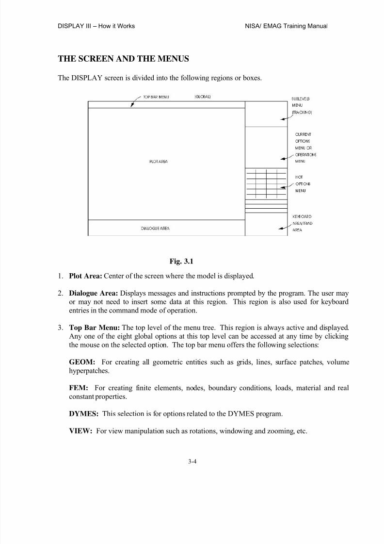
The DISPLAY screen is divided into the following regions or boxes.
1. Plot Area: Center of the screen where the model is displayed.
2. Dialogue Area: Displays messages and instructions prompted by the program. The user mayor may not need to insert some data at this region. This region is also used for keyboardentries in the command mode of operation.
3. Top Bar Menu: The top level of the menu tree. This region is always active and displayed.Any one of the eight global options at this top level can be accessed at any time by clickingthe mouse on the selected option. The top bar menu offers the following selections:
GEOM: For creating all geometric entities such as grids, lines, surface patches, volumehyperpatches.
FEM: For creating finite elements, nodes, boundary conditions, loads, material and realconstant properties.
DYMES: This selection is for options related to the DYMES program.
VIEW: For view manipulation such as rotations, windowing and zooming, etc.
Fig. 3.1

8/12/2019 emagtm
http://slidepdf.com/reader/full/emagtm 27/246
NISA/ EMAG Training Manual DISPLAY III – How it Works
3-5
POST: Provides result interpretation and post-processing options for different analysis.
MISC: Provides miscellaneous options such as layers, sets, device colors, etc.
SET/S: To set or show default parameters that control DISPLAY operation.
FILES: Provides access to all file manipulation options such as read and write of varioustypes of files, ending or restarting in a session.
4. Current Option Menu: This region offers the different options available for furtherexecutions at any stage of the menu operations. At any time, this area reflects the logicalchoices available as next available options depending on the previously performedoperations. At the beginning of a session, the choices in this region coincide with the optionsavailable from the top bar menu. Thereafter, this area displays the dynamically changingoptions available to the user.
GEOM FEM NISA DYMES VIEW POST MISC SET/S FILES
GLOBAL OPTIONS
GEOMETRY OPTIONS
GRIDLINEPATCHHYPERPATCHPLANE PRIMITIVELCS SYSTEM
WORK PLANE NURB CURVESDATA ENTITY
PLO ERA SRH DEL
SVW ORN COL LAB
HLP EXE UND RES
REG CLR WIN PAN
HOT REG UNW COM
KBD ABT
EMRC NISA DISPLAYOCT/01/97 3:03:01
ROTX
ROTY
ROTZ K E Y B O A R D /
T R I A D A R E A
H O T O P T I O N S
M E N U
O P E
R A T I O N
M E N
U
S U B - L E V E L
M E N U

8/12/2019 emagtm
http://slidepdf.com/reader/full/emagtm 28/246
DISPLAY III – How it Works NISA/ EMAG Training Manual
3-6
Suppose we select the GEOM option from the top bar menu as a starting point in creating a patch (surface). Once the top menu GEOM is selected, the current option menuautomatically changes to options available within this GEOM selection. This is shown in
Fig. 3.2.
Now, to create a patch we select the PATCH option from this menu. The programautomatically brings different options available for creation of a patch as a submenu in thisregion. All the selections under this submenu are relevant to creation/modification/copyingor miscellaneous options related to a patch. This is shown in Fig. 3.3.
GEOM FEM NISA DYMES VIEW POST MISC SET/S FILES
GLOBAL OPTIONS
GEOMETRY OPTIONS
GRIDLINEPATCHHYPERPATCHPLANE PRIMITIVELCS SYSTEMWORK PLANE NURB CURVESDATA ENTITY
PLO ERA SRH DEL
SVW ORN COL LAB
HLP EXE UND RES
REG CLR WIN PAN
HOT REG UNW COM
KBD ABT
EMRC NISA DISPLAY
OCT/01/97 3:03:01
ROTX0
ROTY0
ROTZ0
K E Y B O A R D
/
T R I A D A R E A
H O T O P T I O N S
M E N U
O P E R A T I O N
M E N U
S U B - L
E V E L
M E N U
GLOBAL OPTIONS
GEOMETRY OPTIONS
PATCH OPTIONS
CREATECREATE ON GEOMCREATE ON PRIMMODIFYMOVECOPYMISC OPTIONS
PLO ERA SRH DEL
SVW ORN COL LAB
HLP EXE UND RES
REG CLR WIN PAN
HOT REG UNW COM
KBD ABT
EMRC NISA DISPLAY
OCT/01/97 3:03:01
ROTX
0ROTY0
ROTZ0 K
E Y B O A R
D /
T R I A D A R E A
H O T O P T I O N S
M E N U
O P E R A T I O N
M E N U
S U B
- L E V E L
M E N
U
Fig. 3.3
8/12/2019 emagtm
http://slidepdf.com/reader/full/emagtm 29/246
NISA/ EMAG Training Manual DISPLAY III – How it Works
3-7
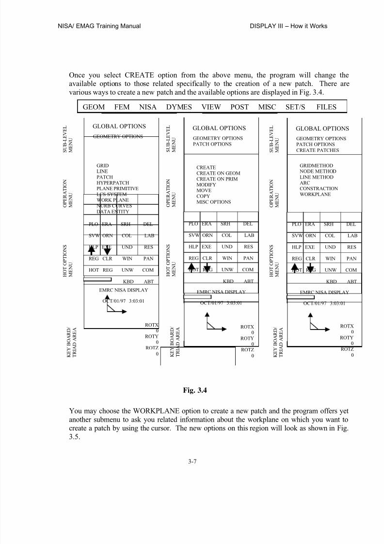
Once you select CREATE option from the above menu, the program will change theavailable options to those related specifically to the creation of a new patch. There are
various ways to create a new patch and the available options are displayed in Fig. 3.4.
You may choose the WORKPLANE option to create a new patch and the program offers yetanother submenu to ask you related information about the workplane on which you want tocreate a patch by using the cursor. The new options on this region will look as shown in Fig.3.5.
GLOBAL OPTIONS
GEOMETRY OPTIONSPATCH OPTIONS
CREATECREATE ON GEOMCREATE ON PRIMMODIFY
MOVECOPYMISC OPTIONS
PLO ERA SRH DEL
SVW ORN COL LAB
HLP EXE UND RES
REG CLR WIN PAN
HOT REG UNW COM
KBD ABT
EMRC NISA DISPLAY
OCT/01/97 3:03:01
ROTX0
ROTY0
ROTZ0 K
E Y B O A R D /
T R I A D A R E A
H O T O P T I O N S
M E N U
O P E R A T
I O N
M E N U
S U B - L E V E L
M E N U
GLOBAL OPTIONS
GEOMETRY OPTIONS
GRIDLINEPATCHHYPERPATCH
PLANE PRIMITIVELCS SYSTEMWORK PLANE NURB CURVESDATA ENTITY
PLO ERA SRH DEL
SVW ORN COL LAB
HLP EXE UND RES
REG CLR WIN PAN
HOT REG UNW COM
KBD ABT
EMRC NISA DISPLAY
OCT/01/97 3:03:01
ROTX0
ROTY0
ROTZ0 K
E Y B O A R D /
T R I A D A R E A
H O T O P T I O N S
M E N U
O P E R A T
I O N
M E N U
S U B - L E V E L
M E N U
GLOBAL OPTIONS
GEOMETRY OPTIONSPATCH OPTIONSCREATE PATCHES
GRIDMETHOD NODE METHODLINE METHODARC
CONSTRACTIONWORKPLANE
PLO ERA SRH DEL
SVW ORN COL LAB
HLP EXE UND RES
REG CLR WIN PAN
HOT REG UNW COM
KBD ABT
EMRC NISA DISPLAY
OCT/01/97 3:03:01
ROTX0
ROTY0
ROTZ0 K
E Y B O A R D /
T R I A D A R E A
H O T O P T I O N S
M E N U
O P E R A T
I O N
M E N U
S U B - L E V E L
M E N U
GEOM FEM NISA DYMES VIEW POST MISC SET/S FILES
Fig. 3.4
8/12/2019 emagtm
http://slidepdf.com/reader/full/emagtm 30/246
DISPLAY III – How it Works NISA/ EMAG Training Manual
3-8
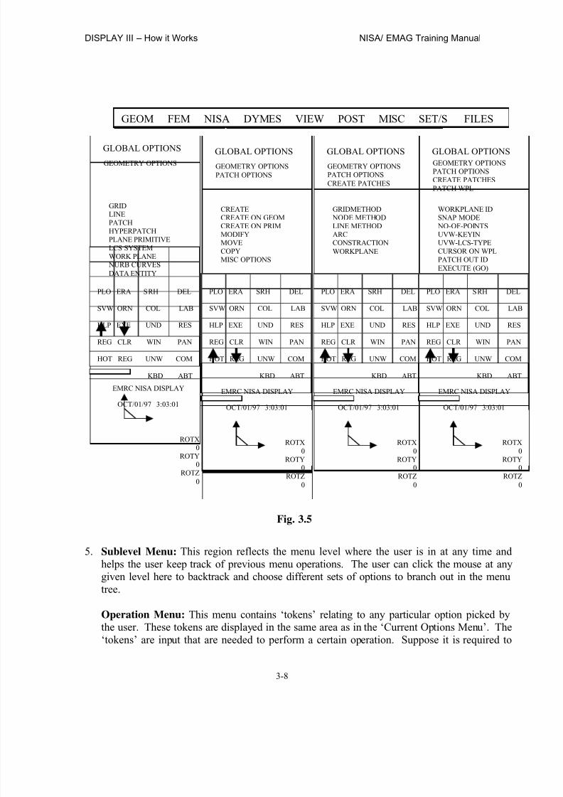
5. Sublevel Menu: This region reflects the menu level where the user is in at any time andhelps the user keep track of previous menu operations. The user can click the mouse at anygiven level here to backtrack and choose different sets of options to branch out in the menutree.
Operation Menu: This menu contains ‘tokens’ relating to any particular option picked bythe user. These tokens are displayed in the same area as in the ‘Current Options Menu’. The‘tokens’ are input that are needed to perform a certain operation. Suppose it is required to
GLOBAL OPTIONS
GEOMETRY OPTIONSPATCH OPTIONS
CREATECREATE ON GEOMCREATE ON PRIMMODIFYMOVECOPYMISC OPTIONS
PLO ERA SRH DEL
SVW ORN COL LAB
HLP EXE UND RES
REG CLR WIN PAN
HOT REG UNW COM
KBD ABT
EMRC NISA DISPLAY
OCT/01/97 3:03:01
ROTX0
ROTY0
ROTZ0
GLOBAL OPTIONS
GEOMETRY OPTIONS
GRIDLINEPATCHHYPERPATCHPLANE PRIMITIVELCS SYSTEMWORK PLANE NURB CURVESDATA ENTITY
PLO ERA SRH DEL
SVW ORN COL LAB
HLP EXE UND RES
REG CLR WIN PAN
HOT REG UNW COM
KBD ABT
EMRC NISA DISPLAY
OCT/01/97 3:03:01
ROTX0
ROTY0
ROTZ0
GEOM FEM NISA DYMES VIEW POST MISC SET/S FILES
GLOBAL OPTIONS
GEOMETRY OPTIONSPATCH OPTIONSCREATE PATCHES
GRIDMETHOD NODE METHODLINE METHODARCCONSTRACTIONWORKPLANE
PLO ERA SRH DEL
SVW ORN COL LAB
HLP EXE UND RES
REG CLR WIN PAN
HOT REG UNW COM
KBD ABT
EMRC NISA DISPLAY
OCT/01/97 3:03:01
ROTX0
ROTY0
ROTZ0
GLOBAL OPTIONSGEOMETRY OPTIONSPATCH OPTIONSCREATE PATCHESPATCH WPL
WORKPLANE IDSNAP MODE NO-OF-POINTSUVW-KEYINUVW-LCS-TYPECURSOR ON WPLPATCH OUT IDEXECUTE (GO)
PLO ERA SRH DEL
SVW ORN COL LAB
HLP EXE UND RES
REG CLR WIN PAN
HOT REG UNW COM
KBD ABT
EMRC NISA DISPLAY
OCT/01/97 3:03:01
ROTX0
ROTY0
ROTZ0
Fig. 3.5

8/12/2019 emagtm
http://slidepdf.com/reader/full/emagtm 31/246
NISA/ EMAG Training Manual DISPLAY III – How it Works
3-9
translate an existing line to create another new line. It is necessary that the followinginformation is supplied to the program:
a. ID of the line to be translated.
b. ID of the new line to be created.
c. Distance by which the existing line is to be translated in each global direction (DX, DY, DZ).
The above information needed to perform the translation operation are ‘tokens’ for thetranslation option. Suppose you select the ‘Translate’ option in the ‘Current Level Menu’, the program then automatically displays the related tokens as a part of the ‘Operation Menu’.
Tokens are color coded and are used for the following purposes:
White Tokens: For these tokens, default values are used unless you override them with
values.
Red Tokens: These tokens require user specified data for execution and no default valuesare assumed.
Green Tokens: These tokens result in execution with user specified input and/or systemdefaults.
Most operation menus have EXECUTE (GO) as the last token. After all other tokens have beenspecified or the default values accepted, you should click this token for execution.
Triad Area: This region on the right hand lower portion of the screen which displays the globalaxes orientation for the model.
Auxiliary Keyboard Area: If the hot button KBD is clicked by the mouse, a numeric keypadappears on top of the triad area as shown in Figure 3.6. This is an auxiliary keyboard, which can be used to insert some numerical values simply by clicking the mouse on different numericvalues. Clicking the KBD hot button at the end of using the keyboard or execution of thecommand will return it to displaying the global triad axis.
7 8 9 , F1 F2 F34 5 6 / F4 F5 F6
1 2 3 – Delete
0 . E + Enter
Fig. 3.6

8/12/2019 emagtm
http://slidepdf.com/reader/full/emagtm 32/246
DISPLAY III – How it Works NISA/ EMAG Training Manual
3-10
Label Boxes: Just above the triad area there are three boxes, which are used for labeling purposes. The topmost box is used to declare the NISA version, the middle box shows the timeand date of your session, and the lowermost box indicates, with a blink, if the program isexecuting a command or not. The yellow dot on the red bar blinks when the program isexecuting a command and remains steady when the program is waiting for further instructions
from the user.
6. Hot Options Menu: This region contains a few “hot” buttons, which can be executed at anytime of the modeling process. These buttons generally provide access to major auxiliarycommands such as aborting execution of a previous command, viewing the model from adifferent angle or simply replotting the whole or part of the model. The options provided inthese hot buttons are executed instantly and the control is returned to the original menu levelwhere the user was before clicking in the hot button. Sometimes a new list of options mayappear in the current level menu as a result of executing a hot button, but it is merely anavailable option for the hot button operation itself. The original current menu level will become active as soon as the hot button operation is performed.
The hot buttons are in two colors — yellow and white. White buttons are “super-hot” in thesense that they can be executed at all times when DISPLAY is waiting for input of any nature,even in the middle of some other operation. Yellow buttons cannot be picked when the programis expecting some other input during execution of another option. Yellow buttons, are alsodifferent in the sense that they usually bring up a list of options to choose from.
The following “hot” buttons are as will look as shown in Figure 3.7 and are described brieflyfollowing the figure.
PLO ERA SRH DELSVW ORN COL LAB
HLP EXE UND RES
RGN CLR WIN PAN
HOT REG UNW COM
↑ ↓ KBD ABT
PLO: Used to plot entities. It opens up another menu and allows you to specify which entities
are to be plotted.
SVW: Allows you to change current viewing angles from a set of standard views such as planview, front/back view, isometric view and other predefined views.
HLP: Offers access to the DISPLAY system help options. The user can select from differenttopics simply by clicking the cursor from selection of help.
Fig. 3.7 Hot button area

8/12/2019 emagtm
http://slidepdf.com/reader/full/emagtm 33/246
NISA/ EMAG Training Manual DISPLAY III – How it Works
3-11
RGN: To regenerate a view on the screen, which is partially rubbed out because ofinsertion/deletion of entities on an existing view.
HOT: Clicking on this button brings up another set of “hot” buttons on the palette as shown inFigure 3.8. As the available options grow in the program, the blank spaces in the palette will be
used to provide more hot buttons in the future.
ERA: To erase entities from the database by selecting another set of options. This enables theuser to temporarily remove unnecessary entities from the active set without actually deletingthem from the database.
ORN: Allows you to change current viewing angles by snapping the cursor on positions from
Fig. 3.8
Fig. 3.9

8/12/2019 emagtm
http://slidepdf.com/reader/full/emagtm 34/246
DISPLAY III – How it Works NISA/ EMAG Training Manual
3-12
the horizontal/vertical/ring bar area. This dynamic viewing option is extremely useful whentrying to view a complicated model from different angles. The change of angles and viewing isinstantaneous. The representation of viewing angles are shown in Figure 3.9.
EXE: Allows execution of user or system defined commands.
CLR: Allows the user to clear the screen and remove everything from the active set. Note thatentities, however, remain in the database.
REG: Allows the user to create a new region on the screen where the plotting should be done.
↑: Allows you to scroll up the dialogue area and see what commands/responses weregiven/obtained from the program in previous operations.
↓ : To scroll the dialogue area down.
SRH: To search and highlight entities of the model.
COL: To change colors of existing entities in the model.
UND: To undo the most recent command that has been executed and is useful whereaccidentally catastrophic instructions were given in the previous command.
WIN: Allows you to create a window by zooming in to a part of the model where magnifiedviews are needed for inspection.
UNW: Allows you to get out of a window and recreate the model as an original, after you have
used the WIN or PAN options.
KBD: This is a toggle, which acts as a switch between the numeric keypad and the global triadaxes display area. More description of this keyboard is available during description of thisnumeric keypad in the later part of this section.
DEL: To delete selected entities from the model. This option opens a menu where selections areto be made for entities, which are to be deleted from the database.
LAB: Is used to set the ID labels of entities as plot ON/plot OFF. If set ON, the correspondingentities will be plotted with their ID numbers on the screen.
RES: Allows you to reset the complete graphics area including the menu areas.
PAN: Allows you to slide a window any direction to enable you to view parts of the model,which are otherwise not visible.
COM: Allows you to switch back to command mode of operations should you prefer to key inthe commands instead of using the menu mode.

8/12/2019 emagtm
http://slidepdf.com/reader/full/emagtm 35/246
NISA/ EMAG Training Manual DISPLAY III – How it Works
3-13
ABT: Allows you to abort the current display option. If you have made a mistake, which is being executed and is taking too long a time, this is a good way to get out of that.
REV: Allows reversing the parametric directions of different entities.
DIR: Used to plot parametric directions of different entities.
QRY: On-line query system used in post-processing. Allows the user to point at entities andobtain the corresponding numeric values.
RCR: To set the recording mode on/off.
EDG: Enables you to plot the edges of the geometric and elemental entities, which are selected,from the menu.
B.C.: This hot option will bring a hot BC-management menu on the fly, which is used tomanage boundary condition data. From a BC-entity set menu, selected boundary condition datacan be erased, plotted, deleted, searched, etc. on the fly. Also a BC-status form gives a complete picture of current boundary conditions.
FAC: Enables you to plot the faces of geometric or elemental entities.
EVA: Brings up the evaluator (scientific calculator) for evaluation of expressions.
Distance between two screen points
To specify whether inside or outside of the box/border to be selected
Set the values of the contours for the contour plots
Ζοοm: To zoom a portion of the screen
To create lines from the grid points selected by the pointing device
For extracting grid points
COM: To toggle between menu mode and command mode
KBD: For activating graphical key board pad
ABT: To abort the current operation
HOT: For toggling between the two hot menus

8/12/2019 emagtm
http://slidepdf.com/reader/full/emagtm 36/246
DISPLAY III – How it Works NISA/ EMAG Training Manual
3-14
‘FORMS’ IN DISPLAY III
In finite element modeling, a good portion of data do not have any graphical meaning and aretherefore, not represented graphically. Element material properties are such an example. Themodel cannot graphically interpret (except showing different colors) the material property values
supplied by the user. In these cases, you will find the need to use ‘FORMS’. Forms enable youto input information without having to remember the command structure and with as little usageof the keyboard as possible. A typical form is shown in Figure 3.10.
You may enter the required data corresponding to boxes and then save/reset and quit from theform. Note that the forms may be very long and you may need to use the horizontal or verticalscroll bars to look for additional data.
MODELING IN COMMAND MODE
In the command mode, you type in valid DISPLAY III commands in the dialogue area of thescreen and interact with the program. You may type in one command at a time or you may alsotype in multiple commands on the same line and execute them at one time.
Fig. 3.10 Material Property Form

8/12/2019 emagtm
http://slidepdf.com/reader/full/emagtm 37/246
NISA/ EMAG Training Manual DISPLAY III – How it Works
3-15
The most general form of DISPLAY III command structure is shown below:
Entry No. 1 2 3 4 5
NAME FUNCTIONS INPUT-ID-LIST OUTPUT-ID-LIST DATA
entry variable/(token) description
1 NAME A valid keyword — usually indicates the type of entity being created, edited or manipulated.
2 FUNCTION Usually indicates the option or function being performedsuch as ADD, DEL, etc.
3 INPUT-ID-LIST The list of existing entities on which the function is being
performed.
4 OUTPUT-ID-LIST The list of IDs for new entities that are being generated.
5 DATA The data used by the command to perform the function.
As an example, let us consider the command:
LIN, TRS, 1, 2, 10
The first entry LIN, is the entity on which the function TRS (Translate) will be performed tomove existing line 1 (input line-ID) by a distance of 10 units in the global X direction (data) tocreate a new line ID 2 (output line ID).
Note that the above is the general form for commands. Most of the commands for creation,manipulation are covered by this form. However, there are some exceptions. To know moreabout the forms of commands, refer to the DISPLAY III User Manuals. You will gain moreinsight in the following sections about use of the command structure.
MODELING WITH SESSION FILES
This useful feature for DISPLAY III allows you to write an ASCII session file input for themodeling session and execute in the batch mode for speedy modeling. The session files areautomatically generated during an interactive session and reside in the working directory asDSP##.SES where ## is a numeric string showing the latest ID of the session file. Keeping thesession files for future use is a smart way of saving a model since these files are relatively small.Experienced users modify the session files to create a model in case of mistakes in previoussessions and then create the model in the batch mode. This saves time and effort for the analyst.
Variable

8/12/2019 emagtm
http://slidepdf.com/reader/full/emagtm 38/246
DISPLAY III – How it Works NISA/ EMAG Training Manual
3-16
CONTROLS OF GRAPHIC DISPLAY
As a user you will have control over the graphics display as to what is displayed on the screenand how it is displayed. The following controls are available:
a) LABELS: These are the IDs assigned to an entity. In most cases you want the program toautomatically assign these numbers. You may display these IDs along with the graphicsrepresentation or you may turn them off.
b) SIZES: The screen size of symbols for certain conditions such as boundary condition, forces,etc. can be controlled by the user.
c) COLOR: Each entity in the program has a unique default color. You may change thesecolors if needed.
d) CURVE AND SURFACE PLOTTING: You may increase the segmentation for plotting
purposes. High values of segmentation will take more time but will draw much smootherlines and surfaces when they are curved.
e) WINDOW/PAN/UNWINDOW: You may zoom into any part of the model to investigatelocal areas of interest. You may also slide or pan a window to view other local areas withoutzooming out.
f) VIEWING TRANSFORMATION: The program offers various options for orienting themodel to obtain the best possible view. You may use continuously changing views or storeyour own selected views to get the best possible views.
g) HIDDEN LINE REMOVAL/BOUNDARY LINE/SHADED IMAGE: To enhance modelvisualization you may obtain plots with hidden lines removed. You may also obtain modelswith only boundaries. This helps locate unwanted cracks in the model.
h) POST PROCESSING: Post processing features within DISPLAY III allows you to readanalysis results files and plot graphs, deformed geometry and contour lines, etc.

8/12/2019 emagtm
http://slidepdf.com/reader/full/emagtm 39/246
NISA/ EMAG Training Manual DISPLAY III – Basic Options for Geometric Modeling
4-1
CHAPTER 4
DISPLAY III — Basic Options for Geometric Modeling
The DISPLAY III basic commands for geometric modeling are described in this section. Thefirst thing to learn will be the ‘entities’ that are supported in the program. These entities arecreated, moved, copied, manipulated and edited through the different operations of the program.The entities can be grouped within different headers in terms of their use as following:
a) Geometric entities: These are entities which are used in the creation of a geometric model.The following are worth mentioning:
GRD: Grids are points in 3D space and are basic building blocks of the model.
LIN: Straight or curved parametric cubic lines created through joining of two or moregrids.
PAT: Patches are geometric entities which define a surface in 3D space. These arerepresented internally as a parametric bi-cubic surface. Elements or nodes for a plate model are created on this surface.
HYP: Hyperpatches are geometric entities which define a volume in 3D space. Theseare represented internally as parametric tricubic solids. Solid meshing is createdon these entities to create a 3D solid model.
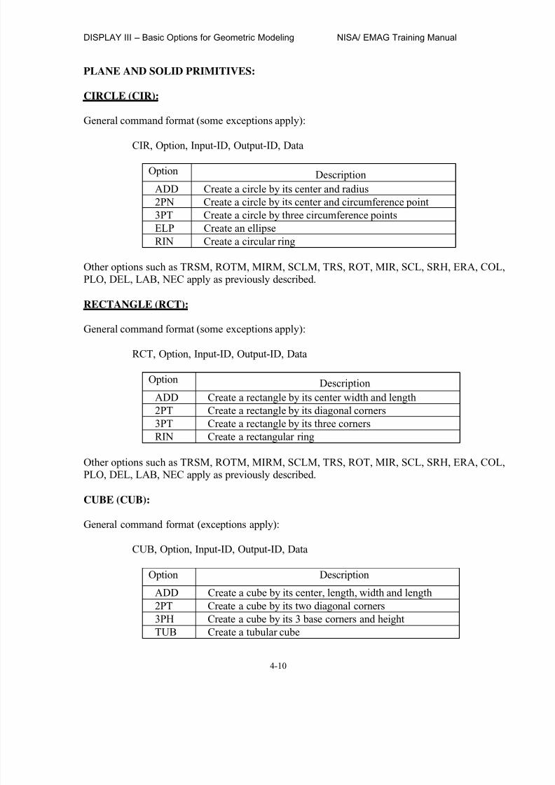
b) Plane Primitives: These are analytically defined 2D shapes which are incorporated within
the program to speed up the modeling process. You can extract geometric entities directlyfrom the primitives and it saves a good amount of time. The following plane primitives arecurrently available in DISPLAY III.
CIR: These are circular shaped primitives to create ellipses, circles and annular rings.
RCT: These are rectangular shaped plane primitives to facilitate creation of rectanglesand squares within the program.
c) Solid Primitives: These are 3D shapes in the program which can be created instantaneously.Geometric entities can be extracted from these primitives for easy modeling.
CYL: Defines shapes of solid cylinder primitives.
SPH: Defines shape of solid spherical primitives.
CON: Defines shape of solid cone primitives. The cones may be truncated, if desired.
CUB: Defines shape of solid parallelepiped primitive.
8/12/2019 emagtm
http://slidepdf.com/reader/full/emagtm 40/246
DISPLAY III – Basic Options for Geometric Modeling NISA/ EMAG Training Manual
4-2
TOR: Defines shape of solid torus primitives to create circular or elliptical shaped torusgeometry.
WED: Defines solid wedge primitives.
PRY: Defines pyramid shapes. The base is defined as an equilateral n-side polygonspecified by its circumcircle or the radius of the inner circle tangent to all sides.
ROD: Defines solid rods with two end holes.
d) Other Entities: Within this subgroup we include special entities which can be created,moved, copied, manipulated and edited within the program.
LCS: The program offers three fundamental coordinate systems: cartesian, cylindricaland spherical, as global coordinate systems. You may create your own local
coordinate system oriented anywhere in space to facilitate model generation.Local coordinate systems may also be created for imposing load and boundaryconditions at some cases. Local coordinate systems are treated as entities whichcan be created, moved, copied, manipulated and edited by the program. There arevarious ways to create a local coordinate system. You should refer to theDISPLAY III User’s Manual for more information.
WPL: A workplane is an infinite plane in 3D space and is designed to facilitate thecreation of planar geometry with maximum use of mouse or other pointingdevices. The workplane can be cartesian or polar type and local cartesian orcylindrical coordinate systems can be defined. Construction points are drawn on
a workplane at increments of local dx and dy distances and the user picks upconstruction points simply by picking the points by the mouse. The density ofinternal construction points as well as the origin and extent of a workplane is usercontrolled. Using workplanes may be a rewarding experience in modeling.
LAY: Layers are used to group some entities of the model under a layer name and thencopied, moved, manipulated or stored. This feature of DISPLAY is extremelyuseful while modeling a large problem.
The DISPLAY functions listed below are global in the sense that they can be used on all of theabove entities (excepting layers). These are the most frequently used options and you may want
to familiarize yourself with their positions in the menu structure. Some of these functions arealso available through the hot buttons. If you prefer to use the command mode, you may want tofind out the command syntax from the DISPLAY manual and keep a copy next to your modelingworkbench.

8/12/2019 emagtm
http://slidepdf.com/reader/full/emagtm 41/246
NISA/ EMAG Training Manual DISPLAY III – Basic Options for Geometric Modeling
4-3
Options for creation or modification of entities:
ADD: Create new entities by providing related data.
TRS: Create new entities by translating existing entities.
TRSM: Modify existing entities by translating (moving) them.
ROT: Create new entities by rotating existing entities about an axis.
ROTM: Modify existing entities by rotating (moving) them.
MIR: Create new entities by mirroring existing entities about a plane.
MIRM: Modify existing entities by mirroring (moving) them.
SCL: Create new entities by scaling existing entities.
SCLM: Modify existing entities by scaling (moving) them.
Options for entity manipulation and image enhancement:
SRH: Search for existing entities and report the database status.
ERA: Erase entities from the screen and remove them from the active set only.
COL: Change color of existing entities for all future plotting.
PLO: Plot entities and add them in the active set.
DEL: Delete existing entities from the database.
LAB: Change label status to turn on/off displaying ID numbers of entities.
NEC: To set new entity color.
SIZ: To set symbol size of entities.
DIS: To find distance between two entities.
DIR: To show parametric direction of geometric entities.
REV: To reverse parametric directions.
In the following pages, you will find a summary of commonly used commands which may beused to create, manipulate and edit different entities.

8/12/2019 emagtm
http://slidepdf.com/reader/full/emagtm 42/246
DISPLAY III – Basic Options for Geometric Modeling NISA/ EMAG Training Manual
4-4
GRIDS (GRD):
General command format (some exceptions apply):
GRD, Option, Input ID, Output ID, Data
Option Description
ADD Create grids by specifying coordinatesWPL Create grids by picking points on workplaneLIN Extract grids from endpoints of existing linesPAT Extract grids from corners of existing patchHYP Extract grids from corners of existing hyperpatchCIR Create grid at the center of an existing circleRCT Create grid at the corners of existing rectangleCUB Create a grid at the corners of existing cubeSPH Create a grid at the center of existing sphereCYL Create grids at the base and top center of cylinder
CON Create grids at the base and top center of a coneTOR Create a grid at the center of an existing torusPYR Create grids at the corners of a pyramidWED Create grids at the corners of a wedgeROD Create grids at the end points of a rod NOD Create a grid at the location of a nodeELE Create grids at the corners of an elementCCL Create a grid at any position of a lineCCP Create a grid at any position of a patchINT Create a grid at the intersection of two lines
LPI Create a grid at intersection of a line and patchTRSM Translate an existing gridROTM Rotate an existing grid about an axisMIRM Mirror an existing grid about a planeSCLM Scale an existing grid about a pointTRS Create a grid by translating an existing gridROT Create a grid by rotating an existing gridMIR Create a grid by mirroring an existing gridSCL Create a grid by scaling a grid about a pointSRH Search for a grid or overall grid statusERA Erase a grid from the active set
COL Reassign color to a set of gridsPLO Plot one or a number of gridsDEL Delete one or many grids from the databaseLAB Plot/not plot grid IDs on the screen NEC Set or change the color of gridsSIZ Change the size of the grid symbol on the screenDIS Find distance between grids
8/12/2019 emagtm
http://slidepdf.com/reader/full/emagtm 43/246
NISA/ EMAG Training Manual DISPLAY III – Basic Options for Geometric Modeling
4-5
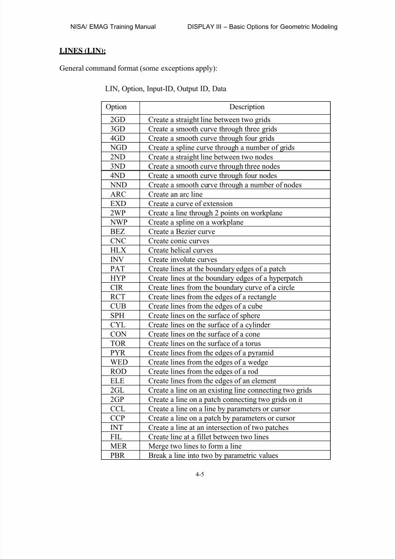
LINES (LIN):
General command format (some exceptions apply):
LIN, Option, Input-ID, Output ID, Data
Option Description
2GD Create a straight line between two grids3GD Create a smooth curve through three grids4GD Create a smooth curve through four grids NGD Create a spline curve through a number of grids2ND Create a straight line between two nodes3ND Create a smooth curve through three nodes4ND Create a smooth curve through four nodes NND Create a smooth curve through a number of nodes
ARC Create an arc lineEXD Create a curve of extension2WP Create a line through 2 points on workplane NWP Create a spline on a workplaneBEZ Create a Bezier curveCNC Create conic curvesHLX Create helical curvesINV Create involute curvesPAT Create lines at the boundary edges of a patchHYP Create lines at the boundary edges of a hyperpatchCIR Create lines from the boundary curve of a circle
RCT Create lines from the edges of a rectangleCUB Create lines from the edges of a cubeSPH Create lines on the surface of sphereCYL Create lines on the surface of a cylinderCON Create lines on the surface of a coneTOR Create lines on the surface of a torusPYR Create lines from the edges of a pyramidWED Create lines from the edges of a wedgeROD Create lines from the edges of a rodELE Create lines from the edges of an element
2GL Create a line on an existing line connecting two grids2GP Create a line on a patch connecting two grids on itCCL Create a line on a line by parameters or cursorCCP Create a line on a patch by parameters or cursorINT Create a line at an intersection of two patchesFIL Create line at a fillet between two linesMER Merge two lines to form a linePBR Break a line into two by parametric values

8/12/2019 emagtm
http://slidepdf.com/reader/full/emagtm 44/246
DISPLAY III – Basic Options for Geometric Modeling NISA/ EMAG Training Manual
4-6
GBR Break a line into two on a specified gridEXT Extend a line along its tangent at the endpointBLE Blend a set of linesTRSM Translate an existing lineROTM Rotate an existing line about an axis
MIRM Mirror an existing line about a planeSCLM Scale an existing line about a pointTRS Create a line by translating an existing lineROT Create a line by rotating a line about an axisMIR Create a line by mirroring a line about a planeSCL Create a line by scaling a line about a pointSRH Search for a line or line statusERA Erase a line from screen and active setCOL Reassign colors to a set of linesPLO Plot a lineDEL Delete a line from the databaseLAB Switch off/on the display of line Ids NEC Set or change the color of linesDIR Find parametric direction of a lineREV Reverse parametric direction of a line
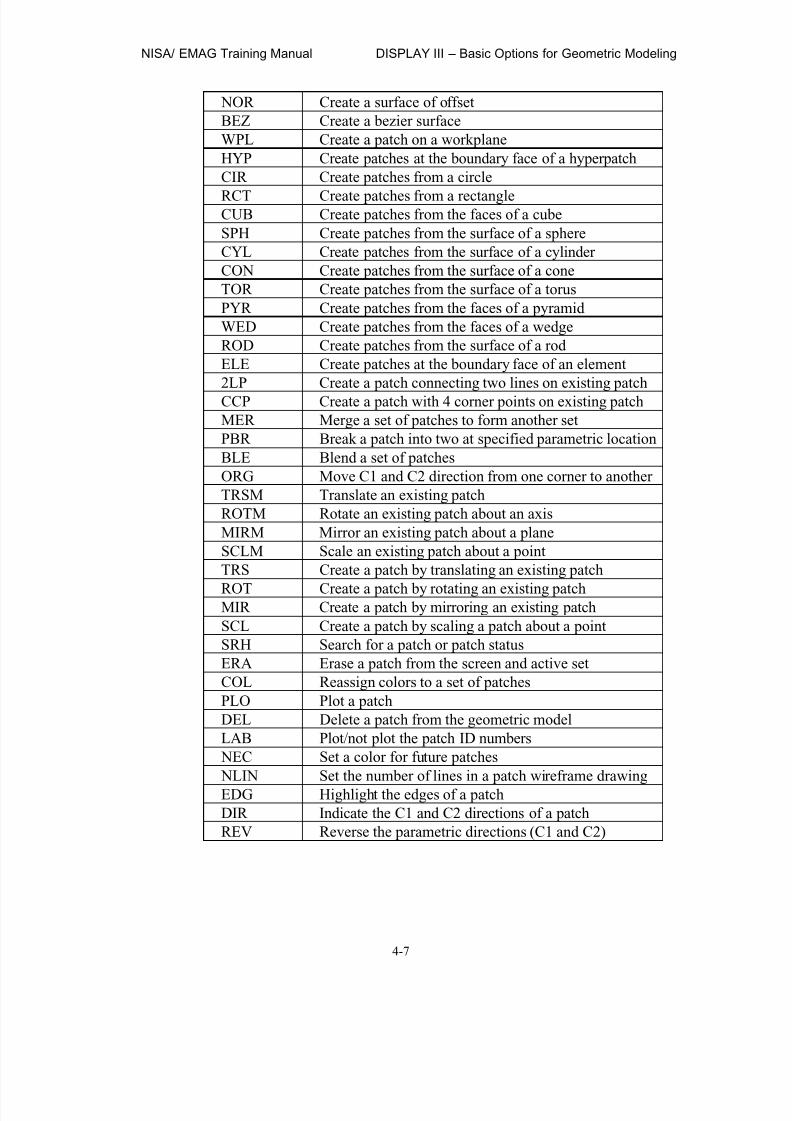
PATCHES (PAT):
The general command format (some exceptions apply):
PAT, Option, Input-ID, Output-ID, Data
Option Description
3GD Create a triangular patch with 3 corner grids4GD Create a patch with 4 corner grids16GD Create a patch through a 4x4 grid mesh3ND Create a triangular patch with 3 corner nodes4ND Create a patch with 4 corner nodes16ND Create a patch through a 4x4 node mesh2LN Create a patch by joining two opposite lines3LN Create a patch by joining 3 lines parallel in space4LN Create a patch by joining 4 lines parallel in space NLN Create a skinning surface through N lines3ED Create a triangular patch with lines as its boundary4ED Create a patch with 4 lines as its boundaryARC Create a surface of revolutionGLI Create a surface by sweepingEXD Create a surface of extrusion
8/12/2019 emagtm
http://slidepdf.com/reader/full/emagtm 45/246
NISA/ EMAG Training Manual DISPLAY III – Basic Options for Geometric Modeling
4-7
NOR Create a surface of offsetBEZ Create a bezier surfaceWPL Create a patch on a workplaneHYP Create patches at the boundary face of a hyperpatchCIR Create patches from a circle
RCT Create patches from a rectangleCUB Create patches from the faces of a cubeSPH Create patches from the surface of a sphereCYL Create patches from the surface of a cylinderCON Create patches from the surface of a coneTOR Create patches from the surface of a torusPYR Create patches from the faces of a pyramidWED Create patches from the faces of a wedgeROD Create patches from the surface of a rodELE Create patches at the boundary face of an element2LP Create a patch connecting two lines on existing patchCCP Create a patch with 4 corner points on existing patchMER Merge a set of patches to form another setPBR Break a patch into two at specified parametric locationBLE Blend a set of patchesORG Move C1 and C2 direction from one corner to anotherTRSM Translate an existing patchROTM Rotate an existing patch about an axisMIRM Mirror an existing patch about a planeSCLM Scale an existing patch about a pointTRS Create a patch by translating an existing patch
ROT Create a patch by rotating an existing patchMIR Create a patch by mirroring an existing patchSCL Create a patch by scaling a patch about a pointSRH Search for a patch or patch statusERA Erase a patch from the screen and active setCOL Reassign colors to a set of patchesPLO Plot a patchDEL Delete a patch from the geometric modelLAB Plot/not plot the patch ID numbers NEC Set a color for future patches NLIN Set the number of lines in a patch wireframe drawingEDG Highlight the edges of a patchDIR Indicate the C1 and C2 directions of a patchREV Reverse the parametric directions (C1 and C2)

8/12/2019 emagtm
http://slidepdf.com/reader/full/emagtm 46/246
DISPLAY III – Basic Options for Geometric Modeling NISA/ EMAG Training Manual
4-8
HYPERPATCHES (HYP):
The general command format (some exceptions apply):
HYP, Option, Input-ID, Output-ID, Data
Option Description
2PA Create hyperpatch by connecting two patches3PA Create hyperpatch by connecting 3 patches parallel in spac4PA Create hyperpatch by connecting 4 patches parallel in spac NPA Create a skinning solid through N patches6PA Create hyperpatch with six boundary patchesARC Create a solid of revolutionGLI Create a solid of sweepEXD Create a solid of extrusion
NOR Create a solid of offsetCUB Create hyperpatches from a cubeSPH Create hyperpatches from a sphereCYL Create hyperpatches from a cylinderCON Create hyperpatches from a coneTOR Create hyperpatches from a torusPYR Create hyperpatches from a pyramidWED Create hyperpatches from a wedgeROD Create hyperpatches from a rodELE Create a hyperpatch from solid elementMER Merge a set of hyperpatches to form a new one
PBR Break a hyperpatch into two at parametric locationsBLE Blend a set of hyperpatchesORG Move the origin of hyperpatch from a corner to otherTRSM Translate an existing hyperpatch about an axisROTM Rotate an existing hyperpatch about an axisMIRM Mirror an existing hyperpatch about a planeSCLM Scale an existing hyperpatch about a pointTRS Create a hyperpatch by translating an existing oneROT Create a hyperpatch by rotating an existing oneMIR Create a hyperpatch by mirroring an existing oneSCL Create a hyperpatch by scaling an existing hyperpatchSRH Search for a hyperpatch or statusERA Erase a hyperpatch from the screen and active setCOL Reassign colors to a set of hyperpatchesPLO Plot a hyperpatchDEL Delete a hyperpatch from the geometric modelLAB Plot/not plot the hyperpatch Ids NEC Set the color of future hyperpatches

8/12/2019 emagtm
http://slidepdf.com/reader/full/emagtm 47/246
NISA/ EMAG Training Manual DISPLAY III – Basic Options for Geometric Modeling
4-9
NLIN Set the number of lines in hyperpatch wireframe plotEDG Highlight the edges of a hyperpatchFAC Highlight the faces of a hyperpatchDIR Indicate the C1, C2 and C3 directions of a hyperpatchREV Reverse the parametric directions of a hyperpatch
LOCAL COORDINATE SYSTEM (LCS):
The general command format is (some exceptions apply):
LCS, Option, Input-ID, Output-ID, Data
Option Description
ADD Create LCS with 3 grids, 3 nodes or 3 coordinatesANG Create LCS by specifying origin and three rotationsVEC Create LCS by specifying origin and two vectors
All other options TRSM, ROTM, MIRM, TRS, ROT, MIR, SRH, ERA, COL, PLO, DEL, LAB,
NEC and SIZE are available for LCS. These are not repeated here and their purposes were
described before.
WORKPLANES (WPL):
The general command format is (some exceptions apply):
WPL, Option, Input-ID, Output-ID, Data
Option Description
ADD Create workplaneDEL Delete user created workplanesPLO Plot a workplaneSRH Search and highlight a workplaneERA Erase a workplaneTRS Translate a workplaneROT Rotate a workplane
MXT Modify extents of a workplaneMDN Modify grid density and grid reference of a workplaneMDS Modify display of a workplaneCOL Change color of a workplaneLAB Switch on/off workplane label plotting NEC Specify new color for future workplanes
8/12/2019 emagtm
http://slidepdf.com/reader/full/emagtm 48/246
DISPLAY III – Basic Options for Geometric Modeling NISA/ EMAG Training Manual
4-10
PLANE AND SOLID PRIMITIVES:
CIRCLE (CIR):
General command format (some exceptions apply):
CIR, Option, Input-ID, Output-ID, Data
Option Description
ADD Create a circle by its center and radius2PN Create a circle by its center and circumference point3PT Create a circle by three circumference pointsELP Create an ellipseRIN Create a circular ring
Other options such as TRSM, ROTM, MIRM, SCLM, TRS, ROT, MIR, SCL, SRH, ERA, COL,PLO, DEL, LAB, NEC apply as previously described.
RECTANGLE (RCT):
General command format (some exceptions apply):
RCT, Option, Input-ID, Output-ID, Data
Option Description
ADD Create a rectangle by its center width and length
2PT Create a rectangle by its diagonal corners3PT Create a rectangle by its three cornersRIN Create a rectangular ring
Other options such as TRSM, ROTM, MIRM, SCLM, TRS, ROT, MIR, SCL, SRH, ERA, COL,PLO, DEL, LAB, NEC apply as previously described.
CUBE (CUB):
General command format (exceptions apply):
CUB, Option, Input-ID, Output-ID, Data
Option Description
ADD Create a cube by its center, length, width and length2PT Create a cube by its two diagonal corners3PH Create a cube by its 3 base corners and heightTUB Create a tubular cube

8/12/2019 emagtm
http://slidepdf.com/reader/full/emagtm 49/246
NISA/ EMAG Training Manual DISPLAY III – Basic Options for Geometric Modeling
4-11
Other options such as TRSM, ROTM, MIRM, SCLM, TRS, ROT, MIR, SCL, SRH, ERA, COL,PLO, DEL, LAB, NEC apply as previously described.
SPHERE (SPH):
General command format (exceptions apply):
SPH, Option, Input-ID, Output-ID, Data
Option Description
ADD Create a sphere by its center and radius2PT Create a sphere by its center and circumference pointELP Create an ellipsoidCUT Create a truncated sphere
Other options such as TRSM, ROTM, MIRM, SCLM, TRS, ROT, MIR, SCL, SRH, ERA, COL,
PLO, DEL, LAB, NEC, NLIN apply as previously described.
CYLINDER (CYL):
General command format (exceptions apply):
CYL, Option, Input-ID, Output-ID, Data
Option Description
ADD Create a cylinder by its center, radius and height2PR Create a cylinder by its base, top centers and radius3PH Create cylinder by 3 base circumference points and radiusELP Create an elliptical cylinder.TUB Create a tubular cylinder
Other options such as TRSM, ROTM, MIRM, SCLM, TRS, ROT, MIR, SCL, SRH, ERA, COL,PLO, DEL, LAB, NEC, NLIN apply as previously described.
CONE (CON):
General command format (exceptions apply):
CON, Option, Input-ID, Output-ID, Data
Option Description
ADD Create a cone by its base center, radii and height2PR Create a cone by its base, top centers and radiiRHA Create a cone by its taper angleELP Create an elliptical coneTUB Create a tubular cone
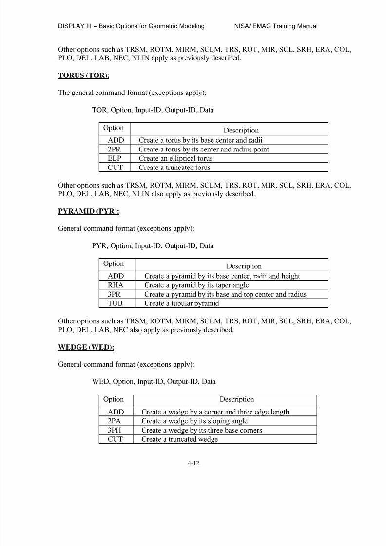
8/12/2019 emagtm
http://slidepdf.com/reader/full/emagtm 50/246
DISPLAY III – Basic Options for Geometric Modeling NISA/ EMAG Training Manual
4-12
Other options such as TRSM, ROTM, MIRM, SCLM, TRS, ROT, MIR, SCL, SRH, ERA, COL,PLO, DEL, LAB, NEC, NLIN apply as previously described.
TORUS (TOR):
The general command format (exceptions apply):
TOR, Option, Input-ID, Output-ID, Data
Option Description
ADD Create a torus by its base center and radii2PR Create a torus by its center and radius pointELP Create an elliptical torusCUT Create a truncated torus
Other options such as TRSM, ROTM, MIRM, SCLM, TRS, ROT, MIR, SCL, SRH, ERA, COL,PLO, DEL, LAB, NEC, NLIN also apply as previously described.
PYRAMID (PYR):
General command format (exceptions apply):
PYR, Option, Input-ID, Output-ID, Data
Option Description
ADD Create a pyramid by its base center, radii and height
RHA Create a pyramid by its taper angle3PR Create a pyramid by its base and top center and radiusTUB Create a tubular pyramid
Other options such as TRSM, ROTM, MIRM, SCLM, TRS, ROT, MIR, SCL, SRH, ERA, COL,PLO, DEL, LAB, NEC also apply as previously described.
WEDGE (WED):
General command format (exceptions apply):
WED, Option, Input-ID, Output-ID, Data
Option Description
ADD Create a wedge by a corner and three edge length2PA Create a wedge by its sloping angle3PH Create a wedge by its three base cornersCUT Create a truncated wedge

8/12/2019 emagtm
http://slidepdf.com/reader/full/emagtm 51/246
NISA/ EMAG Training Manual DISPLAY III – Basic Options for Geometric Modeling
4-13
Other options such as TRSM, ROTM, MIRM, SCLM, TRS, ROT, MIR, SCL, SRH, ERA, COL,PLO, DEL, LAB, NEC also apply as previously described.
ROD (ROD):
General command format (exceptions apply):
ROD, Option, Input-ID, Output-ID, Data
Option Description
ADD Create a rod by its 2 centers and the end axes2PV Create a rod by its start axis and direction vector3PT Create a rod by start axis and endpoint of end axisCUT Create an one-end rod
Other options such as TRSM, ROTM, MIRM, SCLM, TRS, ROT, MIR, SCL, SRH, ERA, COL,PLO, DEL, LAB, NEC, NLIN also apply as previously described.

8/12/2019 emagtm
http://slidepdf.com/reader/full/emagtm 52/246
DISPLAY III – Basic Options for Geometric Modeling NISA/ EMAG Training Manual
4-14
This page intentionally left blank

8/12/2019 emagtm
http://slidepdf.com/reader/full/emagtm 53/246
NISA/ EMAG Training Manual DISPLAY III – Basic Options for Finite Element Modeling
5-1
CHAPTER 5
DISPLAY III — Basic Options for Finite Element Modeling
Once the geometric modeling is complete, finite element meshes are mapped on the geometricmodel and load and boundary conditions are imposed on the model. At the end of the process, aninput file for the solver is automatically generated by the program.
The basic entities for finite element modeling are ELEMENTS (ELE) and NODES (NOD).Elements and nodes are the building blocks of the discretized model and are created by themeshing operation.
The finite element mesh may be generated in one of the following ways:
1. AUTOMATIC MESH GENERATION (AUTOMESH): This process is used to create
finite element model from a purely geometric definition of the boundary of a structure.
Automatic mesh generation can be used to create meshing for the following types ofmodels:
a) For a 2 Dimensional geometry lying in one plane, meshes can be generated from simpleline models only. Only a merged boundary line is needed for the geometry. The program will automatically create a completely quad or tri-quad mesh according to theuser’s wish. The user may even specify linear or parabolic elements for meshgeneration. The program, by default, will create a non-uniform mesh by creating a finemesh at the location of sharp geometry changes and a coarse mesh at areas of uniform potential gradient. You can also control the meshing by selecting a finer meshing.
MOREOPTIONS
ORDER(Ist quad)
MESHSIZE
GRADEDSIZE
GLOBAL DENSITY (.8)LOCAL DENSITY
FEM
MESH
AUTOMESH
2DFLAT
ENTIREMODEL
As an example, let us consider automesh of a 2D arbitrary shape with local mesh control
(at local density prompt, enter 4/111/1)

8/12/2019 emagtm
http://slidepdf.com/reader/full/emagtm 54/246
DISPLAY III – Basic Options for Finite Element Modeling NISA/ EMAG Training Manual
5-2
The Geometry Consisting of Lines
The Resulting Mesh
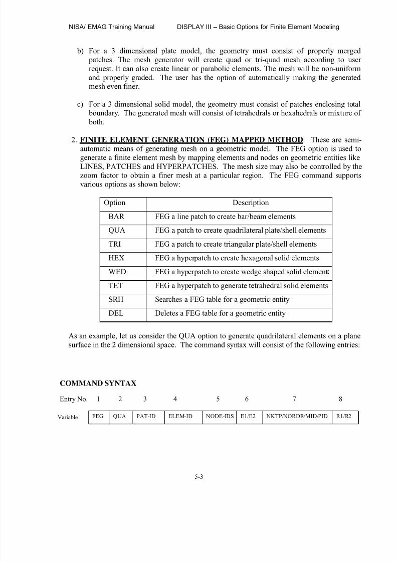
8/12/2019 emagtm
http://slidepdf.com/reader/full/emagtm 55/246
NISA/ EMAG Training Manual DISPLAY III – Basic Options for Finite Element Modeling
5-3
b) For a 3 dimensional plate model, the geometry must consist of properly merged patches. The mesh generator will create quad or tri-quad mesh according to userrequest. It can also create linear or parabolic elements. The mesh will be non-uniformand properly graded. The user has the option of automatically making the generatedmesh even finer.
c) For a 3 dimensional solid model, the geometry must consist of patches enclosing total boundary. The generated mesh will consist of tetrahedrals or hexahedrals or mixture of both.
2. FINITE ELEMENT GENERATION (FEG) MAPPED METHOD: These are semi-automatic means of generating mesh on a geometric model. The FEG option is used togenerate a finite element mesh by mapping elements and nodes on geometric entities likeLINES, PATCHES and HYPERPATCHES. The mesh size may also be controlled by thezoom factor to obtain a finer mesh at a particular region. The FEG command supportsvarious options as shown below:
Option Description
BAR FEG a line patch to create bar/beam elements
QUA FEG a patch to create quadrilateral plate/shell elements
TRI FEG a patch to create triangular plate/shell elements
HEX FEG a hyperpatch to create hexagonal solid elements
WED FEG a hyperpatch to create wedge shaped solid element
TET FEG a hyperpatch to generate tetrahedral solid elements
SRH Searches a FEG table for a geometric entity
DEL Deletes a FEG table for a geometric entity
As an example, let us consider the QUA option to generate quadrilateral elements on a planesurface in the 2 dimensional space. The command syntax will consist of the following entries:
COMMAND SYNTAX
Entry No. 1 2 3 4 5 6 7 8
FEG QUA PAT-ID ELEM-ID NODE-IDS E1/E2 NKTP/NORDR/MID/PID R1/R2Variable
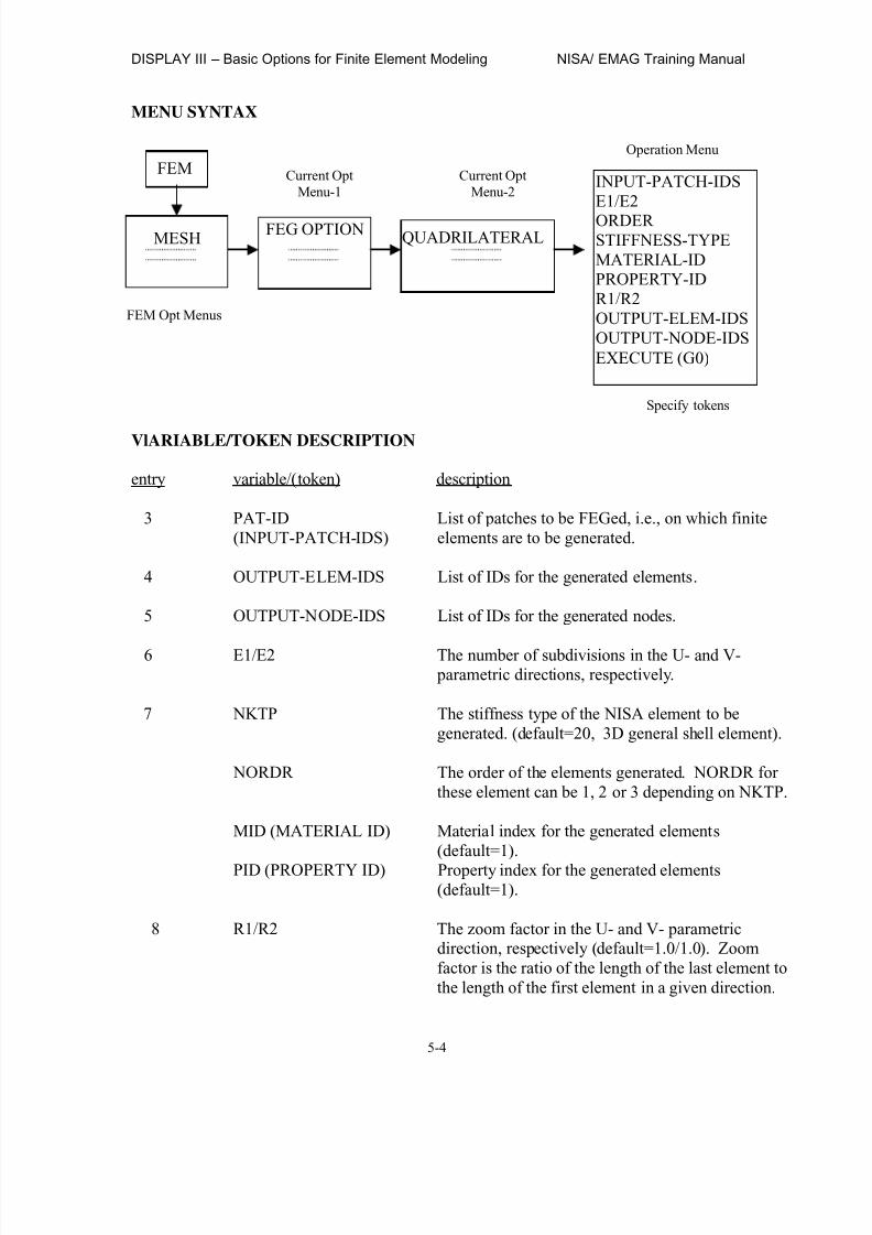
8/12/2019 emagtm
http://slidepdf.com/reader/full/emagtm 56/246
DISPLAY III – Basic Options for Finite Element Modeling NISA/ EMAG Training Manual
5-4
MENU SYNTAX
VlARIABLE/TOKEN DESCRIPTION
entry variable/(token) description
3 PAT-ID List of patches to be FEGed, i.e., on which finite(INPUT-PATCH-IDS) elements are to be generated.
4 OUTPUT-ELEM-IDS List of IDs for the generated elements.
5 OUTPUT-NODE-IDS List of IDs for the generated nodes.
6 E1/E2 The number of subdivisions in the U- and V- parametric directions, respectively.
7 NKTP The stiffness type of the NISA element to begenerated. (default=20, 3D general shell element).
NORDR The order of the elements generated. NORDR forthese element can be 1, 2 or 3 depending on NKTP.
MID (MATERIAL ID) Material index for the generated elements(default=1).
PID (PROPERTY ID) Property index for the generated elements(default=1).
8 R1/R2 The zoom factor in the U- and V- parametricdirection, respectively (default=1.0/1.0). Zoomfactor is the ratio of the length of the last element tothe length of the first element in a given direction.
FEM
MESHFEG OPTION QUADRILATERAL
INPUT-PATCH-IDSE1/E2
ORDERSTIFFNESS-TYPEMATERIAL-IDPROPERTY-IDR1/R2OUTPUT-ELEM-IDSOUTPUT-NODE-IDSEXECUTE (G0)
FEM Opt Menus
Current OptMenu-1
Current OptMenu-2
Operation Menu
Specify tokens

8/12/2019 emagtm
http://slidepdf.com/reader/full/emagtm 57/246
NISA/ EMAG Training Manual DISPLAY III – Basic Options for Finite Element Modeling
5-5
EXAMPLES
To create elements with NORDR=2, NKTP=102 (i.e., eight noded isoparametric elements) using patch 10 with material identification number equal to 1 , and applying zoom factors of 0.3 alongC1 direction and 0.4 along C2 direction, type:
FEG, QUA, 10, , , 2/4, 102/2/1/, 0.3/0.4
3. FINITE ELEMENT GENERATION WITH TOPOLOGICAL ZOOM (FZM):
This is an extension of the FEG command and automates the mesh refinement process.This allows you to create local high densities of mesh and make a smooth transition toareas where the mesh is coarse. The basic command structure is identical to that of theFEG command with a few extra options and a list of locations about which the mesh is to
be refined or ‘zoomed’.

8/12/2019 emagtm
http://slidepdf.com/reader/full/emagtm 58/246
DISPLAY III – Basic Options for Finite Element Modeling NISA/ EMAG Training Manual
5-6
4. FINITE ELEMENT GENERATION WITH AUTOMATED MESH TRANSITION (FAM):
The FAM command is used to generate a finite element mesh on patches andhyperpatches. The command structure is similar to that of the FEG command except thatin this command the user may specify the number of elements desired on each of the four
edges of the patch (and the 3rd parametric direction in the case of a hyperpatch). Thetransitions required to maintain compatibility of elements are automatically generated.You may also individually specify the zoom factors on each of the four edges of the patch(and the 3rd parametric direction for the hyperpatch).
The FAM command supports various options as shown below:
Option Description
QUA to FAM a 4-sided patch and create quad elementsTRI to FAM a 4-sided patch and create triangular elementsHEX to FAM a hpatch and create hexagonal elements
WED to FAM a hpatch and create wedge elements
As an example of the FAM option, let us use the QUA option to create elements on a planesurface in the 2 dimensional space.
To generate FINITE ELEMENT MESH on a patch:
• If you use FEG, you can chose how many elements to create in each direction. (The meshcan be described as A X B elements.)
• If you use FZM, you can create two or four times as many elements along a particular edge.
• FAM gives you an option to create different numbers of elements along all four edges of the patch. Thus, we can generate five elements along edge #1, four along edge #2, three alongedge #3 and two along edge #4. The program takes care of the transition.
COMMAND SYNTAX
Entry No. 1 2 3 4 5 6 7 8
FAM QUA PAT-I ELEM-I NODE-ID E1/E2/E3/E4/IEDT NKTP/NORDR/MID/PI R1/R2/R3/R
Variable
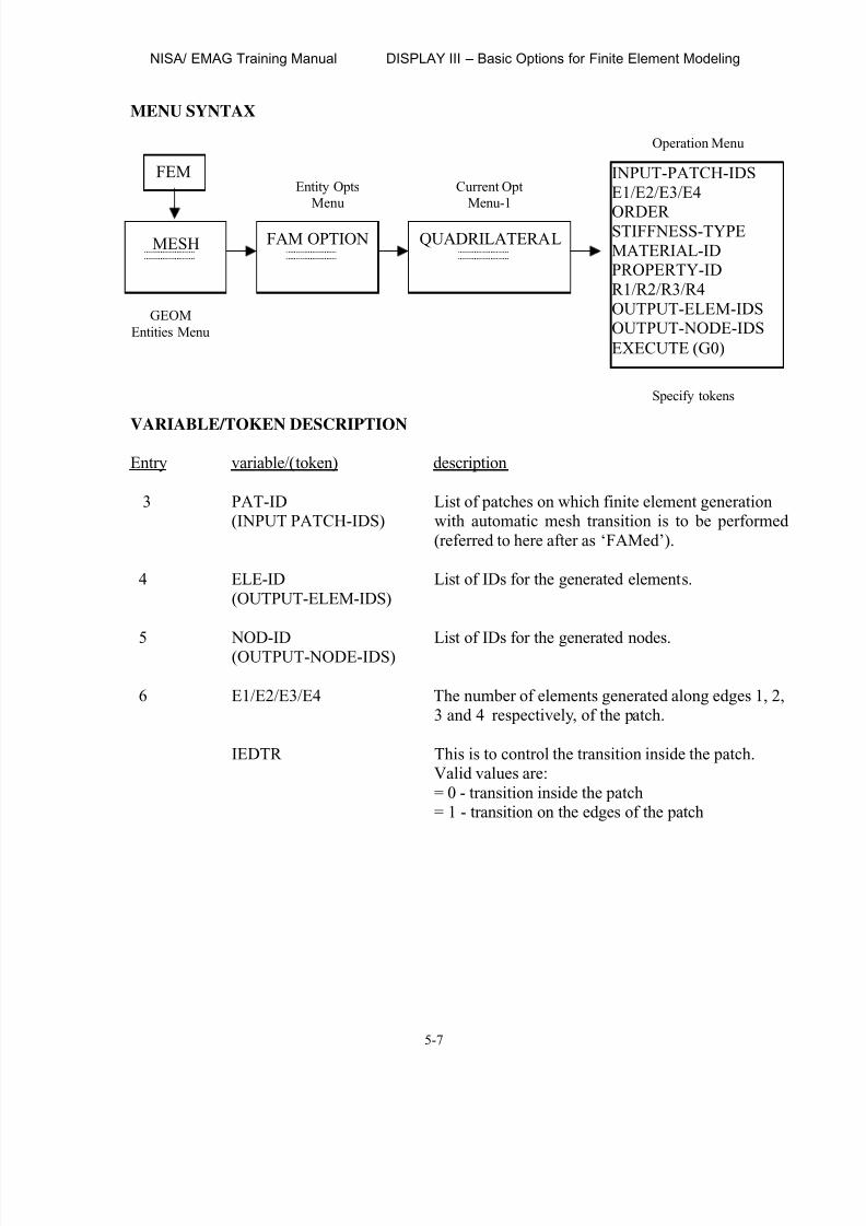
8/12/2019 emagtm
http://slidepdf.com/reader/full/emagtm 59/246
NISA/ EMAG Training Manual DISPLAY III – Basic Options for Finite Element Modeling
5-7
MENU SYNTAX
VARIABLE/TOKEN DESCRIPTION
Entry variable/(token) description
3 PAT-ID List of patches on which finite element generation(INPUT PATCH-IDS) with automatic mesh transition is to be performed
(referred to here after as ‘FAMed’).
4 ELE-ID List of IDs for the generated elements.(OUTPUT-ELEM-IDS)
5 NOD-ID List of IDs for the generated nodes.(OUTPUT-NODE-IDS)
6 E1/E2/E3/E4 The number of elements generated along edges 1, 2,3 and 4 respectively, of the patch.
IEDTR This is to control the transition inside the patch.Valid values are:= 0 - transition inside the patch= 1 - transition on the edges of the patch
FEM
MESH FAM OPTION QUADRILATERAL
INPUT-PATCH-IDSE1/E2/E3/E4
ORDERSTIFFNESS-TYPEMATERIAL-IDPROPERTY-IDR1/R2/R3/R4OUTPUT-ELEM-IDSOUTPUT-NODE-IDSEXECUTE (G0)
GEOMEntities Menu
Entity OptsMenu
Current OptMenu-1
Operation Menu
Specify tokens

8/12/2019 emagtm
http://slidepdf.com/reader/full/emagtm 60/246
DISPLAY III – Basic Options for Finite Element Modeling NISA/ EMAG Training Manual
5-8
entry variable/(token) description
7 NKTP The stiffness type of the NISA element to be generated.(STIFFNESS TYPE) (Default=20 for 3D general shell element).
NORDR The order of the elements generated. NORDR for theseelements can be1, 2 or 3 depending on NKTP.
MID (MATERIALID) Material index for the generated elements (default=1).PID (PROPERTY ID) Property index for the generated elements (default=1).
8 R1/R2/R3/R4 The zoom factor along edges 1, 2, 3, and 4 of the patch(default = 1.0/1.0/1.0/1.0). Zoom factor is the ratio of thelength of the last element to the length of the first elementin a given direction.
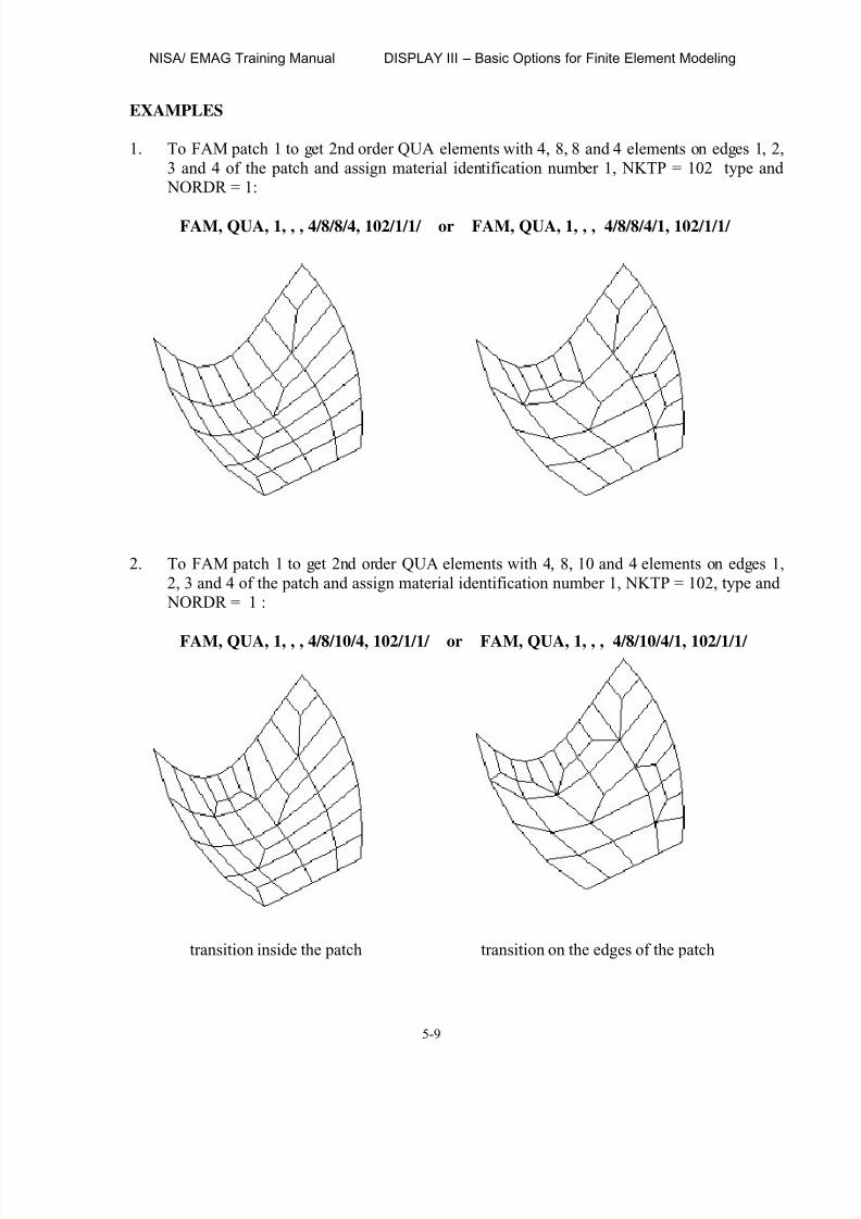
8/12/2019 emagtm
http://slidepdf.com/reader/full/emagtm 61/246
NISA/ EMAG Training Manual DISPLAY III – Basic Options for Finite Element Modeling
5-9
EXAMPLES
1. To FAM patch 1 to get 2nd order QUA elements with 4, 8, 8 and 4 elements on edges 1, 2,3 and 4 of the patch and assign material identification number 1, NKTP = 102 type and NORDR = 1:
FAM, QUA, 1, , , 4/8/8/4, 102/1/1/ or FAM, QUA, 1, , , 4/8/8/4/1, 102/1/1/
2. To FAM patch 1 to get 2nd order QUA elements with 4, 8, 10 and 4 elements on edges 1,2, 3 and 4 of the patch and assign material identification number 1, NKTP = 102, type and NORDR = 1 :
FAM, QUA, 1, , , 4/8/10/4, 102/1/1/ or FAM, QUA, 1, , , 4/8/10/4/1, 102/1/1/
transition inside the patch transition on the edges of the patch

8/12/2019 emagtm
http://slidepdf.com/reader/full/emagtm 62/246
DISPLAY III – Basic Options for Finite Element Modeling NISA/ EMAG Training Manual
5-10
MANIPULATION OF MODEL DATA:
The element and nodes created by the meshing operation are part of the ‘Model Data’ in finiteelement modeling. When a mesh is created by Automesh or FEG/FZM/FAM options, you neednot worry about node or element manipulation much. DISPLAY III, however, offers special
options to create, move, copy, clean, and edit these data. You may never need them, but they areextremely useful in special circumstances.
Node Manipulation
These options shown below:
Optio Description
ADD Create a node with given coordinate dataWPL Create nodes on a workplane
GRD Create nodes at grid locationsCLN Delete all unreferenced nodes from databaseMER Merge nodes within a user specified toleranceDLC Change the displacement local coordinate system of nodeDIS Find distance between two nodes
Other options such as TRS, TRSM, ROT, ROTM, MIR, MIRM, SCL, SCLM, SRH, ERA, COL,PLO, DEL, LAB, NEC, SIZ are also available for nodes and were previously discussed.
Element Manipulation
The available options also include options to verify the quality of the elements and are shown below:
Option Description
ADD Create elements individually by node connectivityREV Reverse nodal connectivity of existing elementsRN Reverse normals of a set of elements w.r.t anotherMPG Change linear elements to parabolic elementsMPR Change parabolic elements to linear elements
MO Modify element parameters and attributesBRK Split a 2D or shell type elements into 2, 3 or 4 elementsRGN Generate solid elements by translating shell elementsCGN Generate solid elements by rotating shell elementsSSG Generate solid elements by offsetting shell elementsDIX Calculate distortion index of elementsCHK Check skewness, warping, aspect ratio and angles of elements

8/12/2019 emagtm
http://slidepdf.com/reader/full/emagtm 63/246
NISA/ EMAG Training Manual DISPLAY III – Basic Options for Finite Element Modeling
5-11
NIS Verify that elements meet NISA requirements NOR Display normal vectors of specified elementsBND Boundary line plot of specified elements or whole modelPAI Paint elements based on material, properties or typeFAC Show element faces
CON Show element connectivity
In addition, other options such as TRS, TRSM, ROT, ROTM, MIR, MIRM, SRH, ERA, COL,PLO, DEL, LAB, NEC are available and were described in earlier chapters.
PHYSICAL PROPERTY SPECIFICATION
Finite element analysis requires physical properties to formulate stiffness matrix. These arematerial properties and will differ for different materials. Material properties are required in allthe elements.
Material properties are also defined through the NISA ‘form’ structure.
Material Properties:
When elements are created in DISPLAY III, a part of their data is in the material-ID. Thematerial-ID, serves as a link between the finite element entities and the actual property values.Required material property values depend on the type of analysis that will be performed.
Material properties are identified by labels. Following is a description of some labels requiredfor Electromagnetic analysis.
Electromagnetic Analysis:
EXX Dielectric permittivity in X direction
EYY Dielectric permittivity in Y direction
EZZ Dielectric permittivity in Z direction
MUXX Permeability in X direction
MUYY Permeability in Y direction
MUZZ Permeability in Z direction
SIXX Electric Conductivity in X direction
SIYY Electric Conductivity in Y direction
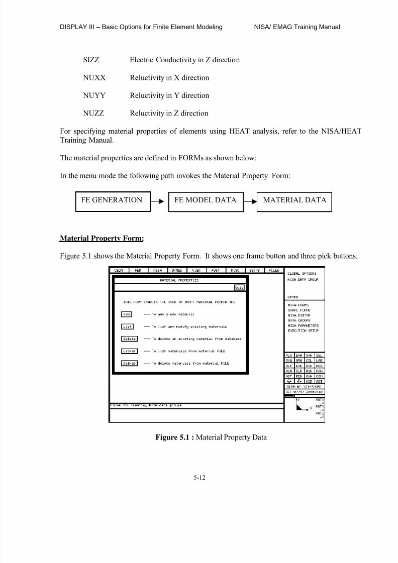
8/12/2019 emagtm
http://slidepdf.com/reader/full/emagtm 64/246
DISPLAY III – Basic Options for Finite Element Modeling NISA/ EMAG Training Manual
5-12
SIZZ Electric Conductivity in Z direction
NUXX Reluctivity in X direction
NUYY Reluctivity in Y direction
NUZZ Reluctivity in Z direction
For specifying material properties of elements using HEAT analysis, refer to the NISA/HEATTraining Manual.
The material properties are defined in FORMs as shown below:
In the menu mode the following path invokes the Material Property Form:
Material Property Form:
Figure 5.1 shows the Material Property Form. It shows one frame button and three pick buttons.
FE GENERATION FE MODEL DATA MATERIAL DATA
Figure 5.1 : Material Property Data
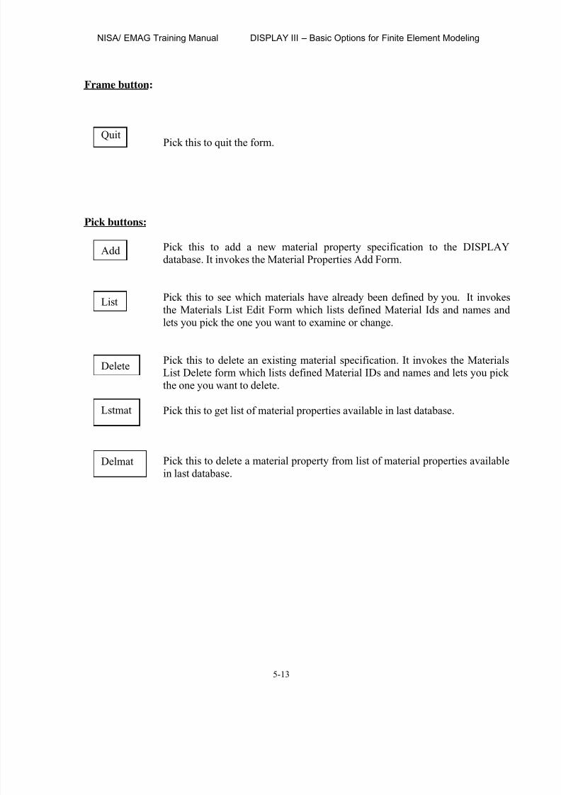
8/12/2019 emagtm
http://slidepdf.com/reader/full/emagtm 65/246
NISA/ EMAG Training Manual DISPLAY III – Basic Options for Finite Element Modeling
5-13
Frame button:
Pick this to quit the form.
Pick buttons:
Pick this to add a new material property specification to the DISPLAYdatabase. It invokes the Material Properties Add Form.
Pick this to see which materials have already been defined by you. It invokesthe Materials List Edit Form which lists defined Material Ids and names andlets you pick the one you want to examine or change.
Pick this to delete an existing material specification. It invokes the MaterialsList Delete form which lists defined Material IDs and names and lets you pickthe one you want to delete.
Pick this to get list of material properties available in last database.
Pick this to delete a material property from list of material properties availablein last database.
Quit
Add
List
Delete
Lstmat
Delmat
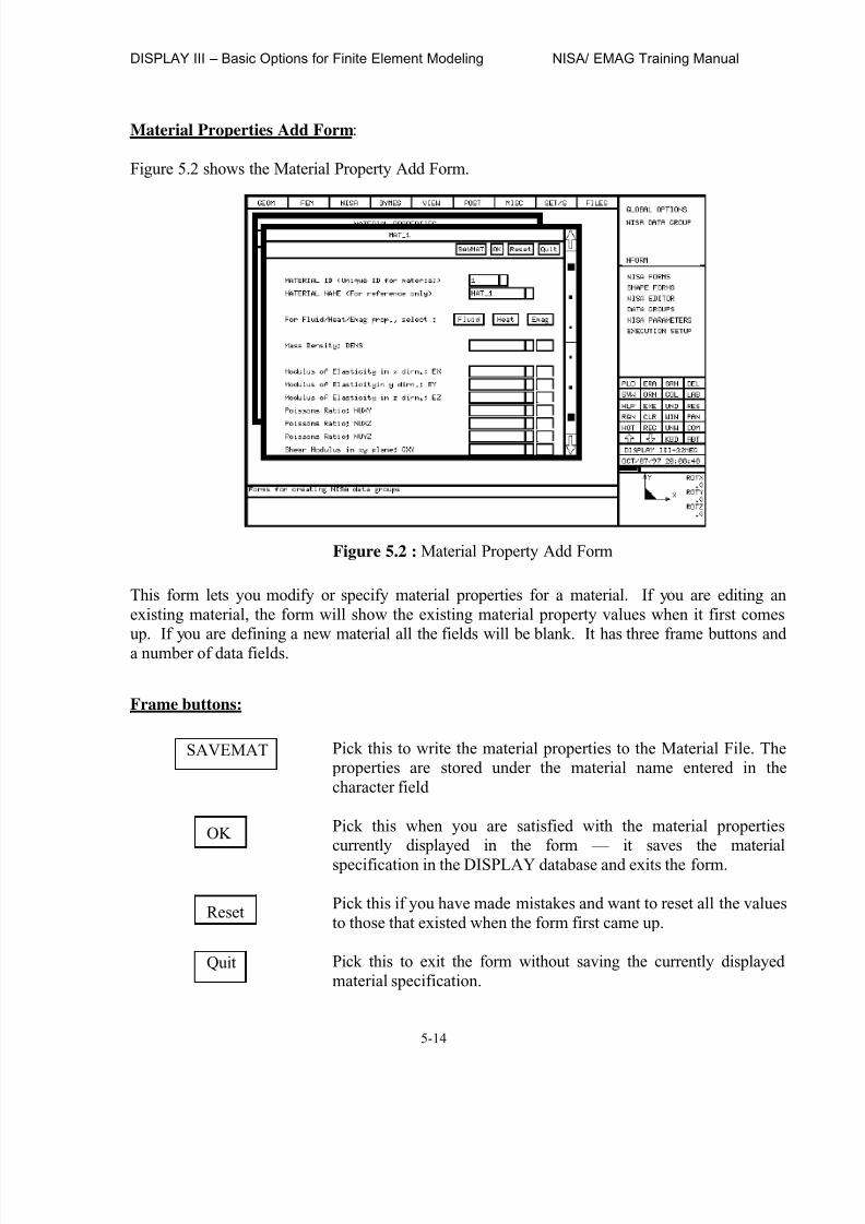
8/12/2019 emagtm
http://slidepdf.com/reader/full/emagtm 66/246
DISPLAY III – Basic Options for Finite Element Modeling NISA/ EMAG Training Manual
5-14
Material Properties Add Form:
Figure 5.2 shows the Material Property Add Form.
This form lets you modify or specify material properties for a material. If you are editing anexisting material, the form will show the existing material property values when it first comesup. If you are defining a new material all the fields will be blank. It has three frame buttons anda number of data fields.
Frame buttons:
Pick this to write the material properties to the Material File. The properties are stored under the material name entered in thecharacter field
Pick this when you are satisfied with the material propertiescurrently displayed in the form — it saves the materialspecification in the DISPLAY database and exits the form.
Pick this if you have made mistakes and want to reset all the valuesto those that existed when the form first came up.
Pick this to exit the form without saving the currently displayedmaterial specification.
SAVEMAT
OK
Reset
Quit
Figure 5.2 : Material Property Add Form
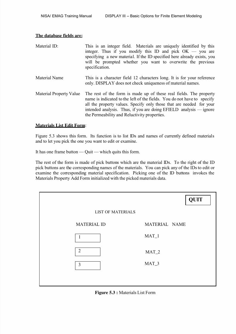
8/12/2019 emagtm
http://slidepdf.com/reader/full/emagtm 67/246
NISA/ EMAG Training Manual DISPLAY III – Basic Options for Finite Element Modeling
5-15
The database fields are:
Material ID: This is an integer field. Materials are uniquely identified by thisinteger. Thus if you modify this ID and pick OK — you are
specifying a new material. If the ID specified here already exists, youwill be prompted whether you want to overwrite the previousspecification.
Material Name This is a character field 12 characters long. It is for your referenceonly. DISPLAY does not check uniqueness of material names.
Material Property Value The rest of the form is made up of these real fields. The propertyname is indicated to the left of the fields. You do not have to specifyall the property values. Specify only those that are needed for yourintended analysis. Thus, if you are doing EFIELD analysis — ignore
the Permeability and Reluctivity properties.
Materials List Edit Form:
Figure 5.3 shows this form. Its function is to list IDs and names of currently defined materialsand to let you pick the one you want to edit or examine.
It has one frame button — Quit — which quits this form.
The rest of the form is made of pick buttons which are the material IDs. To the right of the ID pick buttons are the corresponding names of the materials. You can pick any of the IDs to edit orexamine the corresponding material specification. Picking one of the ID buttons invokes theMaterials Property Add Form initialized with the picked materials data.
QUIT
LIST OF MATERIALS
MATERIAL ID MATERIAL NAME
1
2
3
MAT_1
MAT_2
MAT_3
Figure 5.3 : Materials List Form
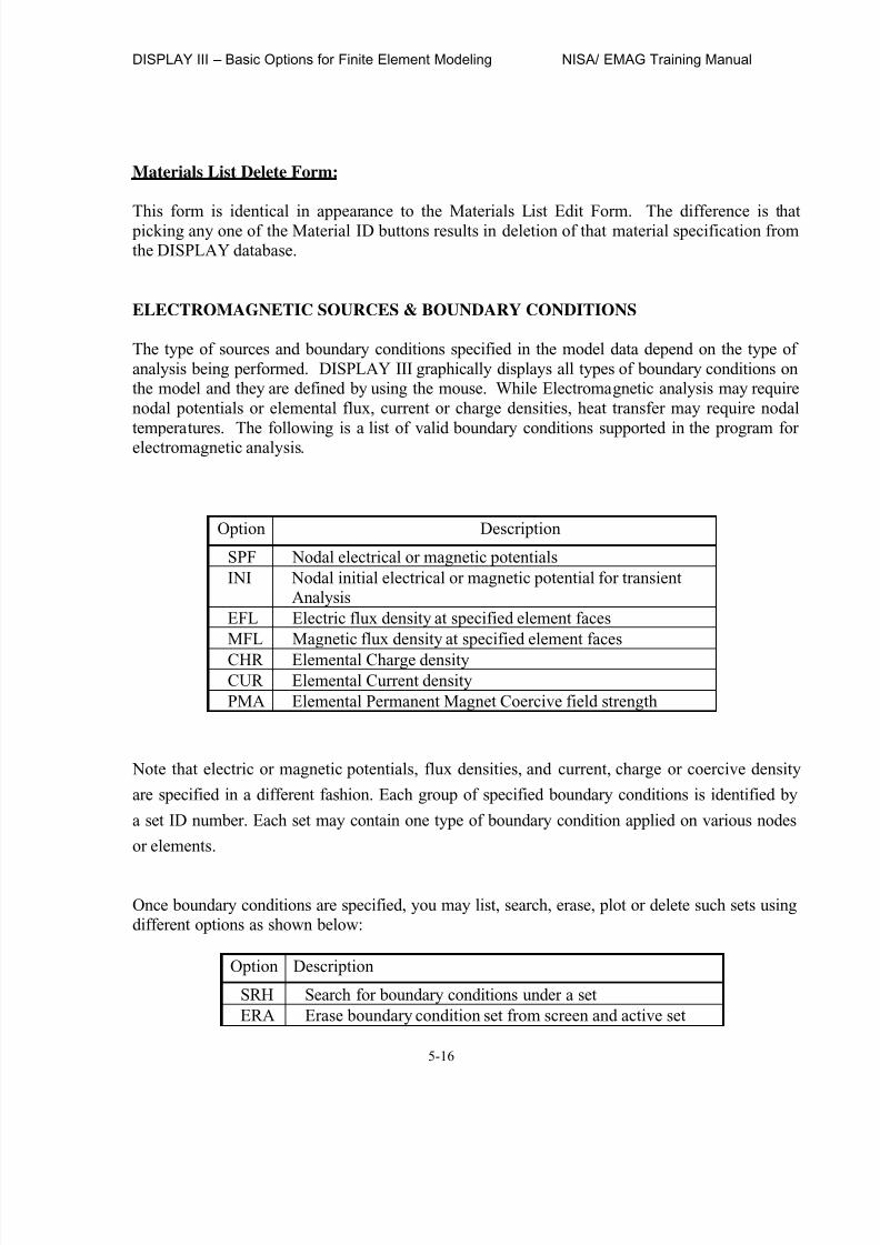
8/12/2019 emagtm
http://slidepdf.com/reader/full/emagtm 68/246
DISPLAY III – Basic Options for Finite Element Modeling NISA/ EMAG Training Manual
5-16
Materials List Delete Form:
This form is identical in appearance to the Materials List Edit Form. The difference is that picking any one of the Material ID buttons results in deletion of that material specification fromthe DISPLAY database.
ELECTROMAGNETIC SOURCES & BOUNDARY CONDITIONS
The type of sources and boundary conditions specified in the model data depend on the type ofanalysis being performed. DISPLAY III graphically displays all types of boundary conditions onthe model and they are defined by using the mouse. While Electromagnetic analysis may requirenodal potentials or elemental flux, current or charge densities, heat transfer may require nodal
temperatures. The following is a list of valid boundary conditions supported in the program forelectromagnetic analysis.
Option Description
SPF Nodal electrical or magnetic potentialsINI Nodal initial electrical or magnetic potential for transient
AnalysisEFL Electric flux density at specified element facesMFL Magnetic flux density at specified element faces
CHR Elemental Charge densityCUR Elemental Current densityPMA Elemental Permanent Magnet Coercive field strength
Note that electric or magnetic potentials, flux densities, and current, charge or coercive density
are specified in a different fashion. Each group of specified boundary conditions is identified by
a set ID number. Each set may contain one type of boundary condition applied on various nodes
or elements.
Once boundary conditions are specified, you may list, search, erase, plot or delete such sets usingdifferent options as shown below:
Option Description
SRH Search for boundary conditions under a setERA Erase boundary condition set from screen and active set

8/12/2019 emagtm
http://slidepdf.com/reader/full/emagtm 69/246
NISA/ EMAG Training Manual DISPLAY III – Basic Options for Finite Element Modeling
5-17
COL Re-assign a color to a boundary condition setPLO Plot a boundary condition set and keep it in active setDEL Delete a boundary conditions setLAB Control plotting of boundary condition set NEC Specify a new color for a boundary condition set
SIZ Set the plotting size of boundary condition set symbol

8/12/2019 emagtm
http://slidepdf.com/reader/full/emagtm 70/246
DISPLAY III – Basic Options for Finite Element Modeling NISA/ EMAG Training Manual
5-18
This page is intentionally left blank
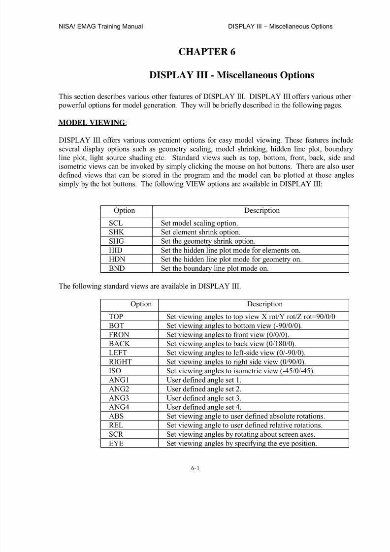
8/12/2019 emagtm
http://slidepdf.com/reader/full/emagtm 71/246
NISA/ EMAG Training Manual DISPLAY III – Miscellaneous Options
6-1
CHAPTER 6
DISPLAY III - Miscellaneous Options
This section describes various other features of DISPLAY III. DISPLAY III offers various other powerful options for model generation. They will be briefly described in the following pages.
MODEL VIEWING:
DISPLAY III offers various convenient options for easy model viewing. These features includeseveral display options such as geometry scaling, model shrinking, hidden line plot, boundaryline plot, light source shading etc. Standard views such as top, bottom, front, back, side andisometric views can be invoked by simply clicking the mouse on hot buttons. There are also userdefined views that can be stored in the program and the model can be plotted at those anglessimply by the hot buttons. The following VIEW options are available in DISPLAY III:
Option Description
SCL Set model scaling option.SHK Set element shrink option.SHG Set the geometry shrink option.HID Set the hidden line plot mode for elements on.HDN Set the hidden line plot mode for geometry on.BND Set the boundary line plot mode on.
The following standard views are available in DISPLAY III.
Option Description
TOP Set viewing angles to top view X rot/Y rot/Z rot=90/0/0BOT Set viewing angles to bottom view (-90/0/0).FRON Set viewing angles to front view (0/0/0).BACK Set viewing angles to back view (0/180/0).LEFT Set viewing angles to left-side view (0/-90/0).RIGHT Set viewing angles to right side view (0/90/0).ISO Set viewing angles to isometric view (-45/0/-45).ANG1 User defined angle set 1.
ANG2 User defined angle set 2.ANG3 User defined angle set 3.ANG4 User defined angle set 4.ABS Set viewing angle to user defined absolute rotations.REL Set viewing angle to user defined relative rotations.SCR Set viewing angles by rotating about screen axes.EYE Set viewing angles by specifying the eye position.

8/12/2019 emagtm
http://slidepdf.com/reader/full/emagtm 72/246
DISPLAY III – Miscellaneous Options NISA/ EMAG Training Manual
6-2
MODEL PARAMETERS
There are several parameters that may need changing depending on the modeling session. Forexample, if the nodal dimensions are too large or too small, the default tolerance parameters fordistance may need to be changed for better modeling practices. These options are available
under SET/SHOW top bar menu. The available options are:
Option Description
TOLD Set tolerance for distance to check equality of points.TOLC Set tolerance for picking entities on screen.SNAP Set snap mode for workplane operations.DWPL Set default workplane ID for workplane operation.ANG1 Assign user defined viewing rotation angle 1.ANG2 Assign user defined viewing rotation angle 2.ANG3 Assign user defined viewing rotation angle 3. NSEG Set number of segments for display of curved lines.CPAI Set point color indexes.LTHK Set line thickness for curve plotting. NCSEG Set number of circular segments to plot circles.CHIDE Set element fill color for hidden line plots.MOUSE Set the definition of mouse.LABA Set the label-ID plotting status for all entities.SCRL Set number of scroll lines in dialogue area.WAIT Set the wait time for PAUSE command in time units.COL Show the current device color indexes.
LAYERS & SETS
DISPLAY III allows you to group certain entities of the model under a layer name and storethese layers in the database for future use. In a similar way, certain entities may be lumped intoa set and given a set ID number.
Layers are identified by a layer name of up to 12 characters and there is no limit on the numberof layers that can be stored in the program. Layers offer various options for creating, modifying,manipulating and editing. These options are listed below:
Option DescriptionADD Create a layer with user defined group of entities.SRH Search for existence of a layer.ERA Erase all entities belonging to a layer from active set.COL Re-assign a color to a particular layer.PLO Plot all entities belonging to a layer.DEL Delete a layer name from database.
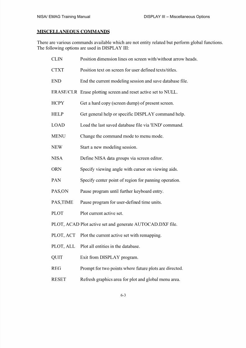
8/12/2019 emagtm
http://slidepdf.com/reader/full/emagtm 73/246
NISA/ EMAG Training Manual DISPLAY III – Miscellaneous Options
6-3
MISCELLANEOUS COMMANDS
There are various commands available which are not entity related but perform global functions.The following options are used in DISPLAY III:
CLIN Position dimension lines on screen with/without arrow heads.
CTXT Position text on screen for user defined texts/titles.
END End the current modeling session and save database file.
ERASE/CLR Erase plotting screen and reset active set to NULL.
HCPY Get a hard copy (screen dump) of present screen.
HELP Get general help or specific DISPLAY command help.
LOAD Load the last saved database file via 'END' command.
MENU Change the command mode to menu mode.
NEW Start a new modeling session.
NISA Define NISA data groups via screen editor.
ORN Specify viewing angle with cursor on viewing aids.
PAN Specify center point of region for panning operation.
PAS,ON Pause program until further keyboard entry.
PAS,TIME Pause program for user-defined time units.
PLOT Plot current active set.
PLOT, ACAD Plot active set and generate AUTOCAD.DXF file.
PLOT, ACT Plot the current active set with remapping.
PLOT, ALL Plot all entities in the database.
QUIT Exit from DISPLAY program.
REG Prompt for two points where future plots are directed.
RESET Refresh graphics area for plot and global menu area.

8/12/2019 emagtm
http://slidepdf.com/reader/full/emagtm 74/246
DISPLAY III – Miscellaneous Options NISA/ EMAG Training Manual
6-4
STATUS Get a quick listing of database entities.
SYSTEM Allow user enter operating system commands.
UNDO Undo the last database changes.
UNW Un-window the last PAN or WIN command action.
WIN Prompt user for window creation and redraw entities.
TEXT EDITING IN DISPLAY III
The pre-processor offers a screen editor within DISPLAY III to edit text files. This is aconvenient editor to perform editing of the NISA input file without getting out of DISPLAY III.The editor comes equipped with frame button search, save, exit and other standard options for a
good screen editor.
MACRO PROGRAMMING IN DISPLAY III
A macro is a set of statements (program) which can be executed in DISPLAY III to modelgeometries in terms of variables and thereby creating parametric models by inserting differentvalues for variables.
Macros use control structures in a fashion similar to any high level programming language. Ifyou enjoy programming, macros will let you add your own commands to DISPLAY.
Macros can be written with all DISPLAY commands and also programming commands likeLABEL, GOTO, CONTINUE, LET, IF, ENDIF, REPEAT, BREAK, LABEL, IF-THEN, ELSE,ENDMACRO.
FILE STRUCTURE:
This section is devoted to explaining the file structure and understanding the significance ofdifferent files and their formats for effective use of the programs. Some of the important filesused for pre\post-processing and analysis are explained below. It is a good practice to use theseextensions when naming a file.
DATABASE FILE (DBS): This file contains the geometry and finite element information for amodel in the binary format. This file is easily retrievable and it is good practice to save such afile during the progression of an interactive session in DISPLAY III thereby avoiding data lossdue to a sudden shutdown of the system.
NEUTRAL FILE (NEU): This file contains either all or selective geometry and finite elementinformation for a model in the ASCII format. Even though this file is not as easily retrievableand occupies more hard disk space than DBS files, it does offer may advantages. The user can

8/12/2019 emagtm
http://slidepdf.com/reader/full/emagtm 75/246
NISA/ EMAG Training Manual DISPLAY III – Miscellaneous Options
6-5
edit a neutral file to make minor changes in the mode. Also, this file is easily transferred fromone computer to another since it is in ASCII format. One major advantage of using a neutral fileis that one can break up a complicated model into different parts and model each partindependently. The user can then read the neutral file associated with each part, one afteranother, into the pre-processor to create the complete model. Neutral files can be written as both
DISPLAY III format as well as DISPLAY II format.
NISA INPUT FILE (NIS): This file is the actual NISA data file which is required for executionof any of the NISA programs. This file can be generated directly from DISPLAY III and thenviewed and edited within it. Since this file is in ASCII format, it is a good idea to view and checkthis file before submitting it for a NISA execution run. This file can also be read into the pre- processor to review and/or modify the model. You are encouraged to become as familiar as possible with the structure of this file since a thorough understanding of this file is necessary tomaster finite element analysis with the NISA family of programs.
SESSION FILE (SES): The pre- and post-processing operations are performed interactively by
the user. Also, the same programs can be executed in a batch mode through the use of sessionfiles. In the pre-processor DISPLAY III, after each session is over the program automaticallysaves a file which has a default name such as DSP#.SES. The character '#' designates the sessionnumber. In post-processing with DISPLAY III, similarly session files are saved as POSTSES.#.These session files contain all the commands that were entered during the session. Often, itseems logical to rename these files and preserve them because they can be read into the pre/post- processor to recreate the model, step by step. These session files are in ASCII format and can,therefore, be edited.
OUTPUT FILE (OUT): This file contains the results from a NISA analysis in ASCII format.This is a standard output file which contains information such as displacements, stresses,reaction forces, strain energy, etc. This file also contains any warning or error messagesgenerated during the analysis. If a NISA execution run crashes, the cause for the programtermination is usually fully documented in this output file. The user has complete control overthe size of this output file through the use of the *SET and *PRINTCNTL cards.
POST PROCESSING FILES (*26.DAT and *39.DAT): These files are the binary output files,which are used in the DISPLAY III post processor DISPLAY-POST for viewing and printing thegraphical results of the problem. These files are saved through the 'SAVE=' and 'FILE='executive cards at the beginning of the NISA input file. For example, in the first modelingsession of this tutorial, files EFIE26.DAT and EFIE39.DAT may have been saved for post- processing because of existence of the following executive cards in the NISA input file, whichwas saved at the end of the modeling session.
SAVE=26,27FILE=EFIE
The file EFIE26.DAT contains geometry information of the model and solutions. At present thefile 39 is not used, but it will be utilized in future versions.
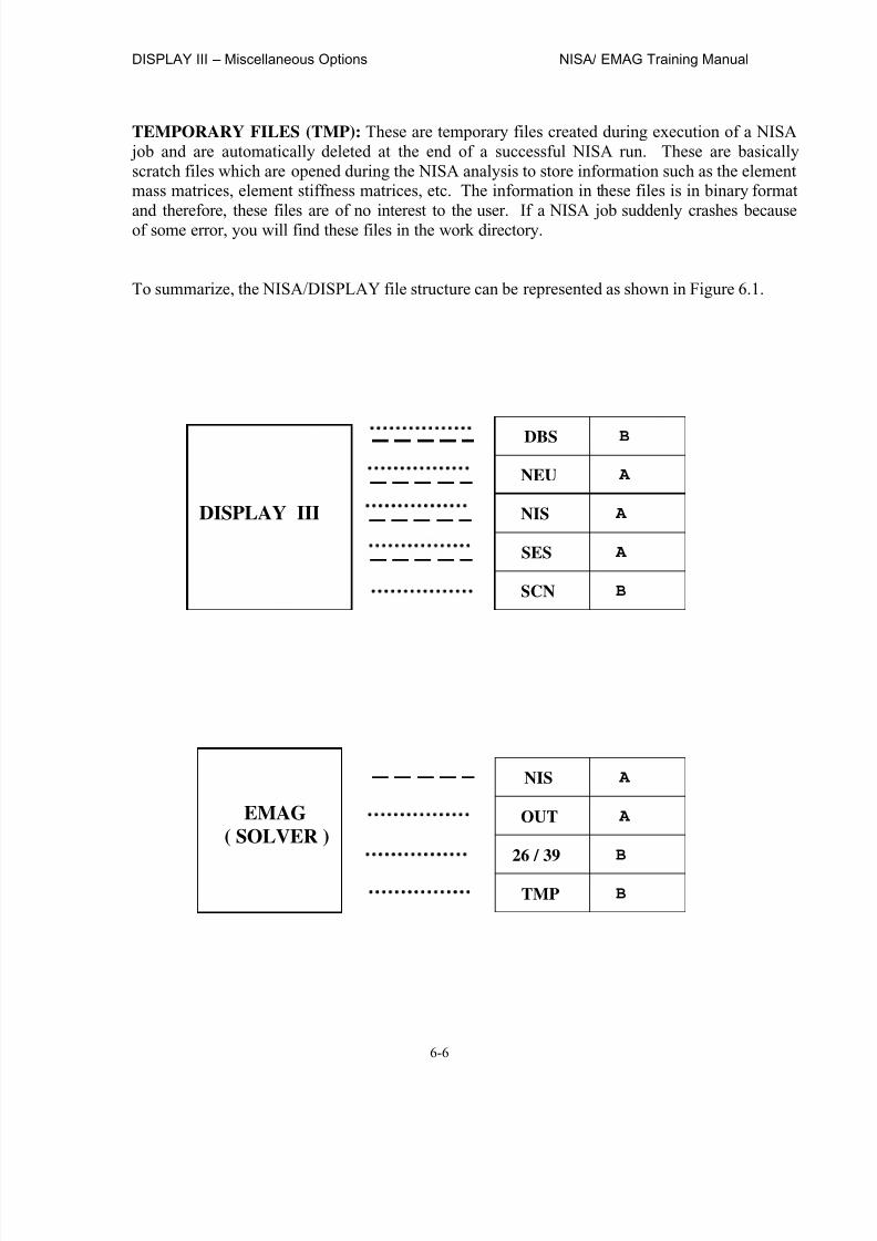
8/12/2019 emagtm
http://slidepdf.com/reader/full/emagtm 76/246
DISPLAY III – Miscellaneous Options NISA/ EMAG Training Manual
6-6
TEMPORARY FILES (TMP): These are temporary files created during execution of a NISA job and are automatically deleted at the end of a successful NISA run. These are basicallyscratch files which are opened during the NISA analysis to store information such as the elementmass matrices, element stiffness matrices, etc. The information in these files is in binary format
and therefore, these files are of no interest to the user. If a NISA job suddenly crashes becauseof some error, you will find these files in the work directory.
To summarize, the NISA/DISPLAY file structure can be represented as shown in Figure 6.1.
DBS B
NEU A
NIS A
SES A
SCN B
NIS A
OUT A
26 / 39 B
TMP B
DISPLAY III
EMAG
( SOLVER )

8/12/2019 emagtm
http://slidepdf.com/reader/full/emagtm 77/246
NISA/ EMAG Training Manual DISPLAY III – Miscellaneous Options
6-7
SES A
SCN B
26 / 39 B
DISPLAY II
( POST )
Fig. 6.1

8/12/2019 emagtm
http://slidepdf.com/reader/full/emagtm 78/246
DISPLAY III – Miscellaneous Options NISA/ EMAG Training Manual
6-8
This page intentionally left blank
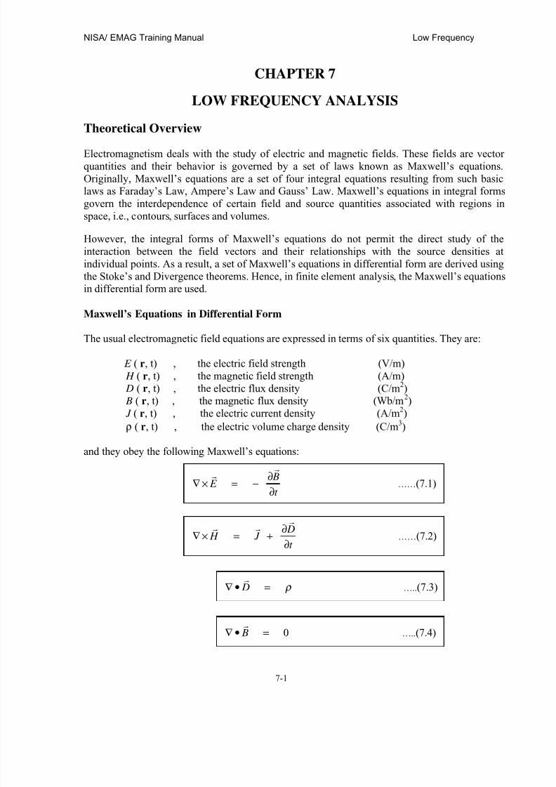
8/12/2019 emagtm
http://slidepdf.com/reader/full/emagtm 79/246
NISA/ EMAG Training Manual Low Frequency
7-1
CHAPTER 7
LOW FREQUENCY ANALYSIS
Theoretical Overview
Electromagnetism deals with the study of electric and magnetic fields. These fields are vectorquantities and their behavior is governed by a set of laws known as Maxwell’s equations.Originally, Maxwell’s equations are a set of four integral equations resulting from such basiclaws as Faraday’s Law, Ampere’s Law and Gauss’ Law. Maxwell’s equations in integral formsgovern the interdependence of certain field and source quantities associated with regions inspace, i.e., contours, surfaces and volumes.
However, the integral forms of Maxwell’s equations do not permit the direct study of theinteraction between the field vectors and their relationships with the source densities atindividual points. As a result, a set of Maxwell’s equations in differential form are derived using
the Stoke’s and Divergence theorems. Hence, in finite element analysis, the Maxwell’s equationsin differential form are used.
Maxwell’s Equations in Differential Form
The usual electromagnetic field equations are expressed in terms of six quantities. They are:
E ( r, t) , the electric field strength (V/m) H ( r, t) , the magnetic field strength (A/m) D ( r, t) , the electric flux density (C/m2) B ( r, t) , the magnetic flux density (Wb/m2)
J ( r, t) , the electric current density (A/m2
)ρ ( r, t) , the electric volume charge density (C/m3)
and they obey the following Maxwell’s equations:
t
B E
∂∂
−=×∇!
!
……(7.1)
t
D J H
∂∂
+=×∇!
!!
……(7.2)
ρ =•∇ D!
…..(7.3)
0=•∇ B!
…..(7.4)

8/12/2019 emagtm
http://slidepdf.com/reader/full/emagtm 80/246
NISA/EMAG Training Manual Low Frequency
7-2
In addition to the above expressions, one needs equations specifying the characteristics of the
medium in which the field exists. These equations are known as the constitutive relations.
The constitutive relations can be written simple as
D = ε E where ε = permittivity (F/m) (7.5) B = µ H where µ = permeability (H/m) (7.6) J = σ E where σ = conductivity (mho/m) (7.7)
In free space void of any matter, σ = 0, ε = ε o and µ = µ o , where, µ o = 4 π x 10-7 H/mε o = 8.854 x 10⁻¹² F/m
The quantities ε, µ and σ are not necessarily simple constants, a notable exception being the
case of ferromagnetic materials for which B – H
relationship may be nonlinear. Furthermore, ε and µ may represent anisotropic materials, in such case the constitutive constants have to bewritten as tensors, i.e.,
Where
The Maxwell’s equation with the constitutive relations include the information contained in theequation of continuity
0=∂∂
+•∇t
J ρ !
…..(7.10)
E D!!
ε = …..(7.8)
H B!!
µ = …..(7.9)
=
z
y
x
ε
ε
ε
ε
00
00
00
;
=
z
y
x
µ
µ
µ
µ
00
00
00
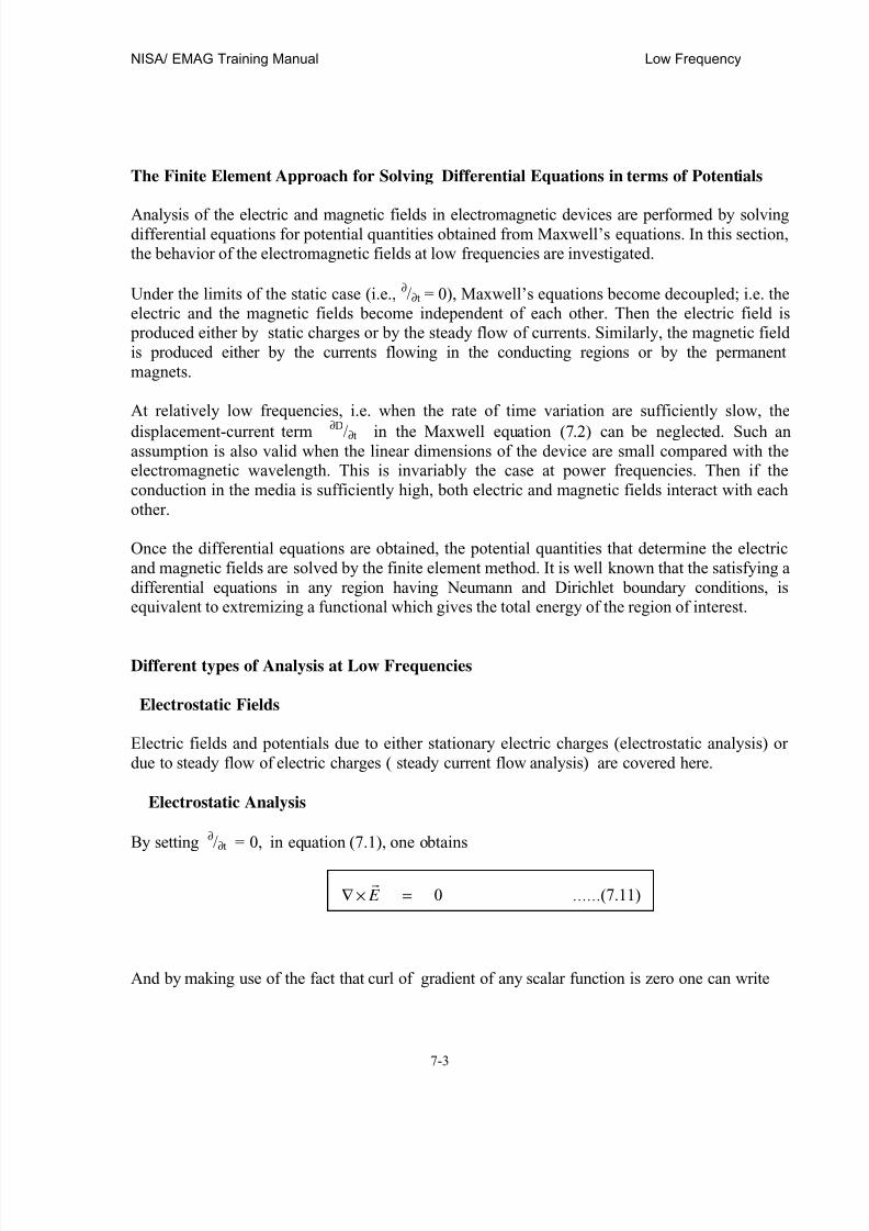
8/12/2019 emagtm
http://slidepdf.com/reader/full/emagtm 81/246
NISA/ EMAG Training Manual Low Frequency
7-3
The Finite Element Approach for Solving Differential Equations in terms of Potentials
Analysis of the electric and magnetic fields in electromagnetic devices are performed by solvingdifferential equations for potential quantities obtained from Maxwell’s equations. In this section,the behavior of the electromagnetic fields at low frequencies are investigated.
Under the limits of the static case (i.e., ∂/∂t = 0), Maxwell’s equations become decoupled; i.e. theelectric and the magnetic fields become independent of each other. Then the electric field is produced either by static charges or by the steady flow of currents. Similarly, the magnetic fieldis produced either by the currents flowing in the conducting regions or by the permanentmagnets.
At relatively low frequencies, i.e. when the rate of time variation are sufficiently slow, the
displacement-current term ∂D/∂t in the Maxwell equation (7.2) can be neglected. Such anassumption is also valid when the linear dimensions of the device are small compared with theelectromagnetic wavelength. This is invariably the case at power frequencies. Then if theconduction in the media is sufficiently high, both electric and magnetic fields interact with eachother.
Once the differential equations are obtained, the potential quantities that determine the electricand magnetic fields are solved by the finite element method. It is well known that the satisfying adifferential equations in any region having Neumann and Dirichlet boundary conditions, isequivalent to extremizing a functional which gives the total energy of the region of interest.
Different types of Analysis at Low Frequencies
Electrostatic Fields
Electric fields and potentials due to either stationary electric charges (electrostatic analysis) ordue to steady flow of electric charges ( steady current flow analysis) are covered here.
Electrostatic Analysis
By setting ∂/∂t = 0, in equation (7.1), one obtains
And by making use of the fact that curl of gradient of any scalar function is zero one can write
0=×∇ E !
……(7.11)

8/12/2019 emagtm
http://slidepdf.com/reader/full/emagtm 82/246
NISA/EMAG Training Manual Low Frequency
7-4
Where φ is known as the electrostatic potential (V). Then, by substituting (7.12) and (7.5) into
(7.4) one obtains the Poisson’s equation for the electric potential.
A space-charge distribution is regarded as given and the boundary condition will often be of theDirichlet type where the potential φ being specified on some boundary surfaces. The natural boundary is of Neumann type, that is, ∂φ/∂n = 0.
The total stored energy is given by
The capacitance of the device is calculated using either
Where V is the voltage difference applied; or
Where Q is the total charge on the conductor and is given by
Where ρs is the surface charge density on the conductor surface S.
Steady Current Flow Analysis
When dealing with conducting materials, the differential equation for the electric scalar
potential can be obtained by making use of the Ohm’s law
φ ∇−= E !
……(7.12)
ρ φ ε −=∇•∇ )( ……(7.13)
)14.7(......21 2 Ω= ∫ Ω
d E W e!
ε
)15.7(......2
2V
W C e=
)16.7(.......2
2
eW
QC =
)17.7(......∫ Ω
=s
sS d Q ρ
)18.7(...... E J !!
σ =

8/12/2019 emagtm
http://slidepdf.com/reader/full/emagtm 83/246
NISA/ EMAG Training Manual Low Frequency
7-5
Where J is the conduction current density and σ is the conductivity of the material.
Consequently, by substituting (7.18) and (7.12) into equation (7.10) and setting ∂/∂t = 0 ,
one can form the Laplace equation
The boundary specification would again commonly be Dirichlet or the natural boundary
condition.
The total dissipated power in the device is given by
And the conductance is calculated using
Where V is the voltage difference applied.
Magnetostatic Fields
Here, the steady magnetic fields produced by the current carrying region and permanent
magnets are stated.
From equation (7.3) and making use of the fact that the divergence of the curl is zero, one
can write
Where A is known as the magnetic vector potential (Wb/m). The differential equation for
the magnetic vector potential A is obtained by substituting (7.22) into (7.2) and then
setting ∂/∂t = 0 ,
)19.7(......0)( =∇•∇ φ σ
)20.7(......
2
Ω= ∫ Ω d
J
Pd σ
!
)21.7(......2
V
PG d =
)22.7(...... A B
!!
×∇=
)23.7......( J A!!
=×∇×∇ ν

8/12/2019 emagtm
http://slidepdf.com/reader/full/emagtm 84/246
NISA/EMAG Training Manual Low Frequency
7-6
Where ν = 1/µ is the reluctivity of the material (m/H). By using vector identities and
the Coulomb’s condition (∇ • A = 0), equation (7.23) can be reduced to the vector
Poisson equation
The total stored magnetic energy is given by
And the inductance of the device is given by
Where I is the current in the conductor and is obtained using
Where J is the current density on the conductor cross section St .
Magnetostatic Analysis for the Translation symmetry Case
For this case, when the current density J and the magnetic vector potential A possess onlylongitudinally directed components; the vector Poisson equation degenerates to its scalarcounterpart
Current density is regarded as given and the boundary condition is of the Dirichlet type where A is specified on some boundary surfaces. The natural boundary condition is Ht = 0.
Magnetostatic Analysis for the Axisymmetric Case
For the axisymmetric case, both the current density J and the magnetic vector potential A possess only θ components; equation (7.23) reduces in the rz plane to
)24.7(......)( J A!!
=∇•∇ ν
)25.7(......2
1 2
Ω= ∫ Ω
d BW h!
ν
)26.7(......2
2
I
W L h=
)27.7(......∫ •=t S
sd J I !
!
)28.7(......)( J A =∇•∇ ν
)29.7(......)(1
J z
A
zr
Ar
r r −=
∂∂
∂∂
+
∂
∂∂∂
ν γ

8/12/2019 emagtm
http://slidepdf.com/reader/full/emagtm 85/246
NISA/ EMAG Training Manual Low Frequency
7-7
The magnetic flux density lies in the rz plane and is related to A by
One can see that the equipotential lines of r A coincide with the flux lines.
Magnetostatic Analysis for the three dimensional Case
The calculation of magnetostatic fields in three dimensions using finite elements can be carriedout using either the full vector potential approach or the reduced scalar potential approach. Thereduced scalar potential method has the inherent advantage over the vector potential method of
having fewer unknowns per node, however, it suffers from what is so-called as the cancellationerror in iron materials near the current carrying regions. Both methods are available in NISA/EMAG for the users to choose the appropriate method for their applications.
The vector potential approach
Governing equation is 7.23. Current density is regarded as given and the boundary condition ofthe Dirichlet type where A is specified on some boundary surfaces.
The reduced scalar potential approach
In many cases the magnetic field intensity H can be separated into two parts
H = H s + H m (7.31)
Where H s is directly the result of the current sources and H m is the magnetization enclosed in thematerial. H s is entirely independent of the material and can be obtained from the Biot-Savartlaw. The vector H m is irrotational, i.e. ,
∇ × H m = 0 (7.32)
Hence, H m can be written as
Where φm is the reduced magnetic scalar potential. A reduced scalar differential equation for the potential can be obtained by using equations (7.31), (7.2) into (7.4) and is given by
( ) )30.7(......
1
)(
1ˆ
^
Ar r r
z Ar zr
r B
∂
∂
+∂
∂
−=
)33.7(......mm H φ ∇−=
( ) ( ) )34.7......(sm H µ φ µ •∇=∇•∇

8/12/2019 emagtm
http://slidepdf.com/reader/full/emagtm 86/246
NISA/EMAG Training Manual Low Frequency
7-8
Where µ is the permeability of the media.
Again, a space-current density is given and the boundary condition is of the Dirichlet type.
Nonlinear magnetic materials
The problem of nonlinearity in magnetostatic analysis can arise when dealing with materialswhose reluctivity depends on the magnetic field. Applications for material nonlinearities areevident for example in performing magnetic field computations in electric machines while takinginto account the saturation effects of the magnetic materials.
To attempt solution of Equation (7.23) by finite element methods, a suitable functional must first be defined. Assuming that the B – H curve for the magnetic material to be monotonicallyincreasing, then the quantity
is recognised as the stored energy density in the magnetization of the material.
Solution Scheme :
The nonlinear magnetostatic analysis is implemented using an iterative procedure based on the Newton-Raphson method.
For nonlinear magnetostatic problems, the stored energy is given by
And the stored coenergy is given by
Problems involving permanent magnets
Here, the solution of problems involving permanent magnet materials with magnetization isconsidered. It is of the form
B = µ ( H + H c ) (7.38)
∫ •= )35.7(.......)( Bd B H nξ
)36.7(......0
Ω
•= ∫ ∫
Ω
d Bd H W
B
h
)37.7(......0
Ω
•= ∫ ∫
Ω
d H d BW
H
c

8/12/2019 emagtm
http://slidepdf.com/reader/full/emagtm 87/246
NISA/ EMAG Training Manual Low Frequency
7-9
Where H c is the coercive field strength of the material. The type of magnetization characteristiccorresponding to (7.38) is shown in Figure (7.1).
B
Nonlinear Permanent Br (remenance)Magnetic Material
Linear PermanentMagnetic Material
- H c H
( magnetic coercivity)
Figure 7.1 Magnetization characteristic for a permanent magnet material.
The vector potential formulation for permanent magnet materials is given by
For linear permanent magnet materials, the material property (reluctivity) is given by
Where H c is the magnetic coercivity and Br is the remenance. While for nonlinear permanentmagnet material, the material property is defined through its demagnetization B – H curveshifted to the first quadrant by H c as shown in Figure (7.2)
)39.7......( J H A c
!!!
=×∇−×∇×∇ ν
)40.7......(r
c
B
H =ν

8/12/2019 emagtm
http://slidepdf.com/reader/full/emagtm 88/246
NISA/EMAG Training Manual Low Frequency
7-10
B
Actual Demagnetization
Curve B – H Demagnetization Curve
- H c H c H
( magnetic coercivity)
Figure 7.2 B – H curve for nonlinear permanent magnet materials.
Analysis of Time-Varying Magnetic Fields
In electromagnetic devices, time-varying currents give rise to time-varying magnetic fields,which in turn induce currents in the conducting materials, called eddy currents. If these currentsare large enough, they can cause numerous problems to the device of interest. In general, eddycurrent time-fluctuation rates are low enough for the simplification of Maxwell’s equations by
neglecting the displacement current ( i.e.,
∂ D
/∂t = 0 ). The differential equation for the magneticvector potential A is then given by
Where ν is the reluctivity of the device and σ the conductivity of the materials present.
The induced eddy currents are given by
For the two-dimensional case ( i.e., J s flowing only in the axial direction ), equation (7.41)reduces to
)41.7(......)(s J
t
A A
!
!
!
=∂∂
+×∇×∇ σ ν
)42.7(......t
A J
e ∂
∂
−= σ
)43.7(......)(s J
t
A A −=
∂∂
−∇•∇ σ ν

8/12/2019 emagtm
http://slidepdf.com/reader/full/emagtm 89/246
NISA/ EMAG Training Manual Low Frequency
7-11
Equation (7.43) is applicable to the general two-dimensional time-varying case where nonlinearmagnetic materials may be present.
Transient Field analysis
In the case of transient excitation J s(t), equation (7.43) is solved using the time integrationmethod. Three different types of time integration schemes are available and are controlled by thetime integration parameter α :
1. Trapezoidal ( Crank-Nicholson ) (α = 0.5 )2. Galerkin (α = 0.67 )3. Backward difference ( Implicit Euler ) (α = 1.0 )
The variation of the excitation can be represented by piecewise linear curves of time vs.amplitude. For accurate results it is important that the time-step ∆t should be sufficiently fine.
Hence, the size of the time steps can be fixed or varying. This time step method can also dealwith nonlinear problems.
Time-Harmonic Field Analysis (Magnetodynamic Analysis)
When considering the case in which J s represents a time-harmonic excitation at frequency ω (rad/s) and ν corresponding to a linear material (steady with time), equation (7.43) can be writtenas
Where A and J s are now complex quantities.
The impedance per unit length of the device is given by
Z = R + j ω L (7.45)
R is the resistance of the conductor and is calculated using
Where Pd is the dissipated power in the conductor and I is the total current in the conductor. L isthe inductance of the conductor and is calculated using
Where Wh is the total stored energy.
)44.7(.......)( s J A j A −=−∇•∇ σ ω ν
)46.7(......2
I
P R d =
)47.7(......2
2 I
W L h=
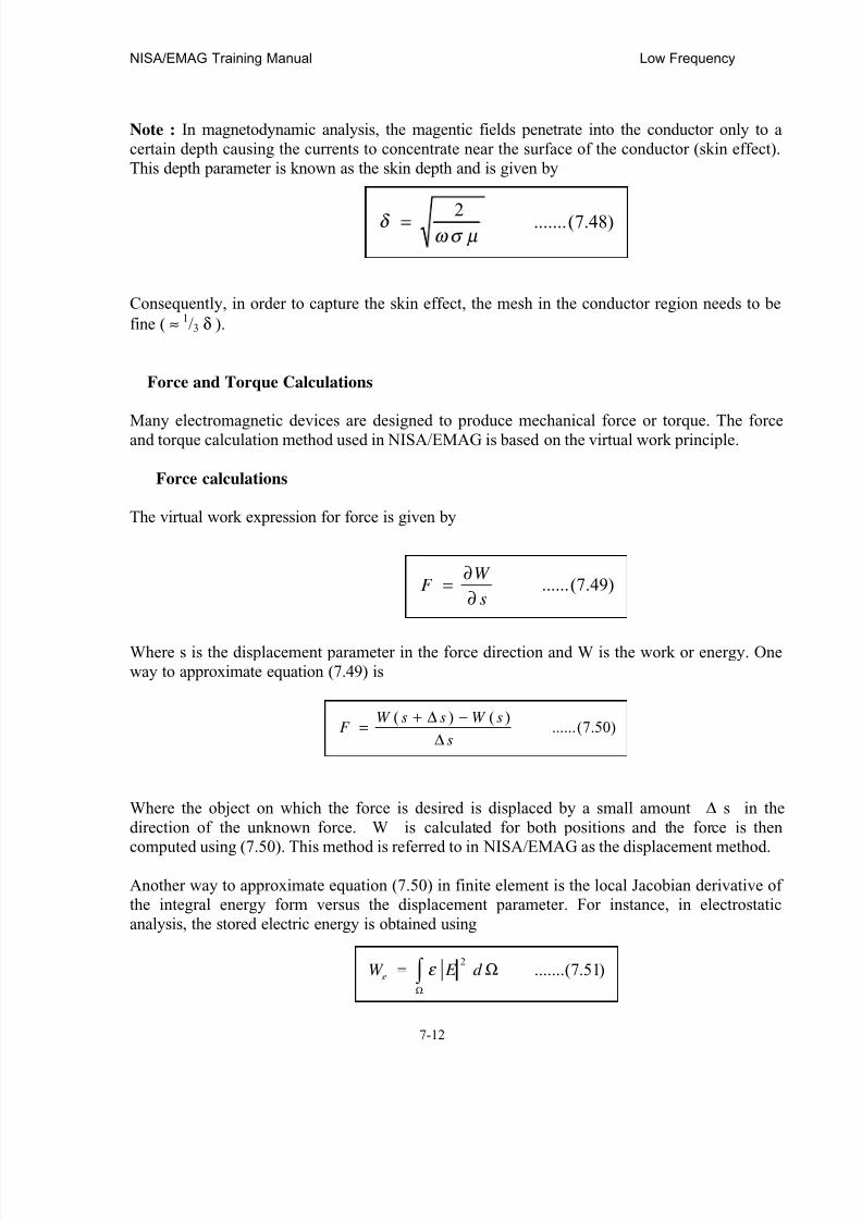
8/12/2019 emagtm
http://slidepdf.com/reader/full/emagtm 90/246
NISA/EMAG Training Manual Low Frequency
7-12
Note : In magnetodynamic analysis, the magentic fields penetrate into the conductor only to acertain depth causing the currents to concentrate near the surface of the conductor (skin effect).This depth parameter is known as the skin depth and is given by
Consequently, in order to capture the skin effect, the mesh in the conductor region needs to befine ( ≈ 1/3 δ ).
Force and Torque Calculations
Many electromagnetic devices are designed to produce mechanical force or torque. The forceand torque calculation method used in NISA/EMAG is based on the virtual work principle.
Force calculations
The virtual work expression for force is given by
Where s is the displacement parameter in the force direction and W is the work or energy. Oneway to approximate equation (7.49) is
Where the object on which the force is desired is displaced by a small amount ∆ s in thedirection of the unknown force. W is calculated for both positions and the force is then
computed using (7.50). This method is referred to in NISA/EMAG as the displacement method.
Another way to approximate equation (7.50) in finite element is the local Jacobian derivative ofthe integral energy form versus the displacement parameter. For instance, in electrostaticanalysis, the stored electric energy is obtained using
)48.7(.......2µ σ ω
δ =
)49.7(......s
W F
∂∂
=
)50.7(......)()(
s
sW ssW F
∆−∆+
=
)51.7(.......2
∫ Ω
Ω= d E W e ε

8/12/2019 emagtm
http://slidepdf.com/reader/full/emagtm 91/246
NISA/ EMAG Training Manual Low Frequency
7-13
The electrostatic force can then be calculated using
This method is referred to in NISA/EMAG as the volume integration method.
The magnetic forces in nonlinear magnetostatic problems are more accurately computed with theaid of the stored coenergy, i.e. ,
Where Wc is the stored coenergy and s is the displacement parameter of the moving object.
In addition, NISA/EMAG computes the Lorentz forces in the current carrying regions using
Where, J is the current density, B is the magnetic flux density and ΩJ is the volume of thecurrent carrying region
Torque calculations
Similar to force calculations, torque calculations in electric motors, generators and other rotatingdevices are carried out using the virtual work principle, i.e. ,
Where Wc is the stored coenergy in the device and θ is the angular displacements of the
rotating object in radians. Both the displacement method and the volume integration method areused for the torque calculations in NISA/EMAG.
Coupled Magneto-Thermal Analysis
The presence of currents in electromagnetic devices (conduction currents, eddy currents)
)52.7(.......2
∫ Ω
∂
∂= d E
s
F e ε
)53.7(......s
W F c
h ∂∂
=
)54.7(.......∫ Ω
Ω×= J
d B J F !!!
)55.7(........θ ∂
∂= cW
T
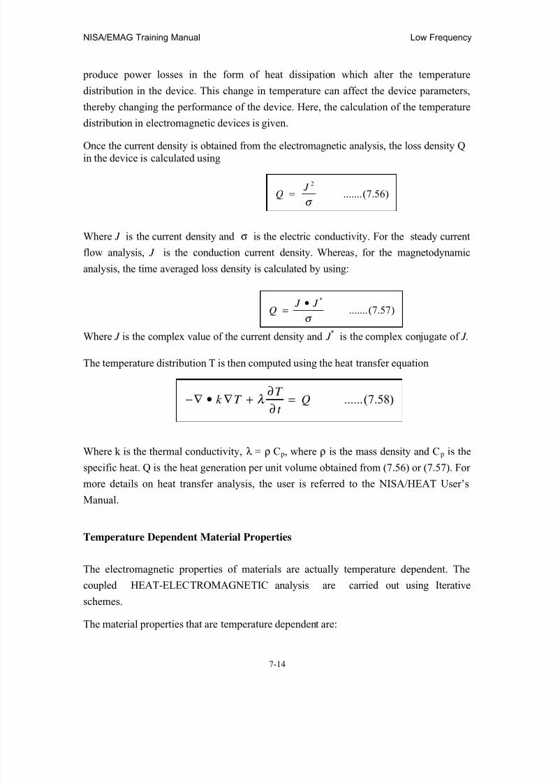
8/12/2019 emagtm
http://slidepdf.com/reader/full/emagtm 92/246
NISA/EMAG Training Manual Low Frequency
7-14
produce power losses in the form of heat dissipation which alter the temperature
distribution in the device. This change in temperature can affect the device parameters,
thereby changing the performance of the device. Here, the calculation of the temperature
distribution in electromagnetic devices is given.
Once the current density is obtained from the electromagnetic analysis, the loss density Qin the device is calculated using
Where J is the current density and σ is the electric conductivity. For the steady current
flow analysis, J is the conduction current density. Whereas, for the magnetodynamic
analysis, the time averaged loss density is calculated by using:
Where J is the complex value of the current density and J * is the complex conjugate of J.
The temperature distribution T is then computed using the heat transfer equation
Where k is the thermal conductivity, λ = ρ C p, where ρ is the mass density and C p is the
specific heat. Q is the heat generation per unit volume obtained from (7.56) or (7.57). For
more details on heat transfer analysis, the user is referred to the NISA/HEAT User’s
Manual.
Temperature Dependent Material Properties
The electromagnetic properties of materials are actually temperature dependent. The
coupled HEAT-ELECTROMAGNETIC analysis are carried out using Iterative
schemes.
The material properties that are temperature dependent are:
)56.7(.......2
σ
J Q =
)57.7(.......*
σ
J J Q
•=
)58.7(......Q
t
T T k =
∂
∂+∇•∇− λ

8/12/2019 emagtm
http://slidepdf.com/reader/full/emagtm 93/246
NISA/ EMAG Training Manual Low Frequency
7-15
1. Permittivity2. Permeability (Reluctivity)3. Conductivity
The variation of these properties with respect to temperature can be given in two ways:
1. Polynomial function2. Tabular Form
Infinite Element
The correct solution of an electromagnetic problem is obtained when the governingequation is solved along with the specified boundary conditions. Most of the real lifeelectromagnetic problems possess open geometry in full or part of their problem domain.This is because some of the boundary conditions are specified only at the boundary of theunbounded domain and these regions have therefore to be considered. Some example ofthese boundary conditions are the electrostatic potential φ and components of themagnetic vector potential A. In all these cases, value of this boundary condition is zero, because the electromagnetic fields at a point in the unbounded region varies roughly asthe reciprocal of the distance between that point and the electromagnetic sources presentin the problem. When the distance becomes large the fields tend to zero. If the problem isconsidered theoretically the field value at the open boundary is exactly zero, since thedistance is infinitely large. When the finite element method is used to solve the problem,one has to truncate the open boundary to achieve a practical problem region that can bemodeled. The truncation has to be judiciously decided.
The reduction of the modeling effort and the computation time can be considerable wheninfinite elements are used. At all portions of the open boundary infinite elements are placed. The shape function of these elements is chosen in such a way that the fields decayalong the outward direction of the open boundary. By a proper selection of the decay parameters, it is possible to reasonably match the field decay with that actually present inthe original problem. Alternatively, the usual shape function of the finite elements can beretained in the infinite element, but the portion of the infinite element lying on the open boundary can be made to approach infinity.
NISA/EMAG both the approaches for the infinite element have been used.
Infinite elements have been implemented for all analysis and sub-analysis types.
The classes of elements available are : 1. Element with Exponential Decay of potential 2. Element with Reciprocal decay of potential 3. Element with geometry mapped to infinity

8/12/2019 emagtm
http://slidepdf.com/reader/full/emagtm 94/246
NISA/EMAG Training Manual Low Frequency
7-16
The type of elements available are :
1. For Two-dimensional problems with NKTP = 101 and 102
and NORDR = 1 and 2
2. For Axisymmetric problems with NKTP = 103
and NORDR = 1 and 2
3. For Three-dimensional problems with NKTP = 104 and 105
and NORDR = 1 and 2
EMAG CAPABILITIES
Electric Field Analysis ( EFIELD )
Electric field analysis in electromagnetic devices induced by :a. Static charge distribution or static voltage distribution - ESTAT b. Steady state flow of electric charges or DC current - SCFL
Electrostatics ( ESTAT )
Electric field calculations in dielectric materials due to specified :1. Static electric charges2. Voltage distribution
Inputs :
- Specified static electric charges or voltage distribution or both
Outputs :- Electrostatic potential distribution- Electric field intensity distribution- Electric flux density distribution- Stored electric energy for each element- Total stored electric energy- Capacitance
Post processing is available for the potential, electric field intensity and the electric
flux density
Typical Problems:1. Capacitors2. Electrostatic precipitator3. Transmission lines4. Multi-conductor distribution with specified voltages5. Transformers and wall bushings
8/12/2019 emagtm
http://slidepdf.com/reader/full/emagtm 95/246
NISA/ EMAG Training Manual Low Frequency
7-17
6. Outdoor insulators7. Supporting insulator blocks8. Design of corona shields9. Dielectric breakdown in High Voltage Engineering problems
Steady state current flow ( SCFL )
Electric field calculations in conducting materials due to specified:1. Steady flow of electric charges or DC current2. Voltage distribution
Inputs:- Specified steady flow of electric charges ( DC current ) or voltage distribution
or both
Outputs:
- Electrostatic potential distribution- Electric field intensity distribution- Current density distribution- Dissipated power for each element- Total dissipated power- Conductance
Post processing is available for the potential, electric field intensity and the currentdensity
Typical Problems:1. Particle counter in Tomography2. Particle detection in Bio-Medical Engineering3. Resistance of arbitrary shaped conductors
Magnetic Field Analysis ( MFIELD )
Magnetic field analysis in electromagnetic devices with direct current ( dc ) sources or time
varying current sources ( alternating ( ac ) or transient ). The magnetic material can be linear,
saturable ( nonlinear ) and / or permanent magnet
Magnetostatics
Magnetic field calculations in magnetic materials due to specified :1. Direct current ( dc ) excitation2. Permanent magnet

8/12/2019 emagtm
http://slidepdf.com/reader/full/emagtm 96/246
NISA/EMAG Training Manual Low Frequency
7-18
Types:1. 2 D planar and Axisymmetric Magnetostatic analysis using the magnetic vector
potential approach ( MGSV ).2. 3 D Magnetostatic analysis using the reduced scalar potential approach (MGSS)3. 3 D Magnetostatic analysis using the magnetic vector potential approach
( MGVP )Inputs:Specified direct current ( dc ) or permanent magnets or both
Outputs :- Magnetic vector potential or scalar potential distribution- Magnetic Flux density distribution- Magnetic field distribution- Stored magnetic energy and coenergy for each element- Magnetic force or torque ( when applicable )- Total stored magnetic energy and coenergy
- Inductance
Post processing is available for the magnetic vector potential or magnetic scalar potential,magnetic field intensity and the magnetic flux density.
Typical Problems:1. Solenoids2. Transmission lines3. Transformers4. D C Machines5. Circuit breakers6. Relays, Etc.
Magnetodynamics ( MGDN )
Magnetic field calculations in magnetic and conducting materials due to specified:Sinusoidal current ( ac ) excitation
Inputs:Specified Sinusoidal current ( ac )
Outputs:- Magnetic vector potential distribution- Magnetic Flux density distribution- Magnetic field distribution- Eddy current density distribution- Total current density distribution- Electric field distribution due to Eddy currents
8/12/2019 emagtm
http://slidepdf.com/reader/full/emagtm 97/246
NISA/ EMAG Training Manual Low Frequency
7-19
- Total Electric field distribution- Power loss density distribution- Stored magnetic energy density for each element- Total stored magnetic energy- Total power loss
- Inductance- Resistance
Post processing is available for the magnetic vector potential, magnetic field intensity,magnetic flux density, eddy current density, total current density and instantaneous (orsnapshots ) time results
Typical Problems:1. Solenoids2. Transmission lines and bus bars3. Transformers
4. Induction Machines5. Synchronous Machines
Transient Magnetic Field Analysis ( TMAG )
Magnetic field calculations in magnetic and conducting materials due to specifiednon-Sinusoidal current ( ac ) excitation
Inputs:Specified arbitrary current excitation
Outputs :- Magnetic vector potential distribution- Magnetic Flux density distribution- Magnetic field distribution- Induced Eddy current density distribution- Electric field distribution due to Eddy currents- Power loss density distribution- Stored magnetic energy and coenergy for each element- Total stored magnetic energy and coenergy
Post processing is available for the magnetic vector potential , magnetic field intensity ,magnetic flux density at different time steps
Typical Problems:1. Solenoids2. Induction furnace3. Transformers4. Induction Machines5. Synchronous Machines

8/12/2019 emagtm
http://slidepdf.com/reader/full/emagtm 98/246
NISA/EMAG Training Manual Low Frequency
7-20
Coupled EMAG - HEAT Analysis
Coupled Heat transfer analysis in electromagnetic devices due to the power losscaused by the applied and induced currents. This analysis can be carried out coupling
heat with steady state current flow analysis, magnetostatics, transient magnetic fieldanalysis and magnetodynamic analysis. You can define the material properties asfunction of temperature.
Outputs:- Thermal and electric/magnetic field distributions.
Typical Problems:1. Solenoids2. Transformers3. Induction furnace
4. Electric furnace5. Induction Machines6. Synchronous Machines
Other Important Capabilities
Infinite elements:
a. Are available for all Analysis types. b. Three types of infinite elements are available :
1. Exponential Decay type2. Reciprocal Decay type3. Mapped element type
c. Infinite elements are available for :1. NKTP = 101, 102, 103, 104 and 105 and
NORDR = 1 and 2
Temperature Function:
Material properties can be defined as functions of temperature for CoupledHEAT analysis.
Tetrahedral Elements:
Tetrahedral elements are now available for 3 D analysis.
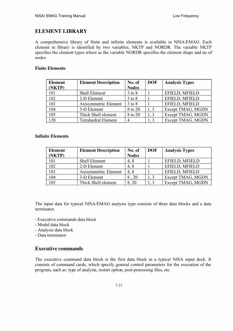
8/12/2019 emagtm
http://slidepdf.com/reader/full/emagtm 99/246
NISA/ EMAG Training Manual Low Frequency
7-21
ELEMENT LIBRARY
A comprehensive library of finite and infinite elements is available in NISA/EMAG. Eachelement in library is identified by two variables, NKTP and NORDR. The variable NKTPspecifies the element types where as the variable NORDR specifies the element shape and no of
nodes.
Finite Elements
Element
(NKTP)
Element Description No. of
Nodes
DOF Analysis Types
101 Shell Element 3 to 8 1 EFIELD, MFIELD102 2-D Element 3 to 8 1 EFIELD, MFIELD103 Axisymmetric Element 3 to 8 1 EFIELD, MFIELD104 3-D Element 8 to 20 1, 3 Except TMAG, MGDN
105 Thick Shell element 8 to 20 1, 3 Except TMAG, MGDN120 Tetrahedral Element 4 1, 3 Except TMAG, MGDN
Infinite Elements
Element
(NKTP)
Element Description No. of
Nodes
DOF Analysis Types
101 Shell Element 4, 8 1 EFIELD, MFIELD102 2-D Element 4, 8 1 EFIELD, MFIELD
103 Axisymmetric Element 4, 8 1 EFIELD, MFIELD104 3-D Element 8 , 20 1, 3 Except TMAG, MGDN105 Thick Shell element 8, 20 1, 3 Except TMAG, MGDN
The input data for typical NISA/EMAG analysis type consists of three data blocks and a dataterminator.
- Executive commands data block- Model data block
- Analysis data block- Data terminator
Executive commands
The executive command data block is the first data block in a typical NISA input deck. Itconsists of command cards, which specify general control parameters for the execution of the program, such as: type of analysis, restart option, post-processing files, etc.

8/12/2019 emagtm
http://slidepdf.com/reader/full/emagtm 100/246
NISA/EMAG Training Manual Low Frequency
7-22
These are the list of executive commands used in NISA/3D-EMAG.
ANALYSIS Specifies analysis typeBLANK Specifies Blank common storage limit
CHEAT Specifies Coupled Magneto-Thermal analysisELEMENT ECHO Echoes element inputEXECUTION Selects execution / checking runFILE NAME Specifies NISA file prefixINITIAL POTENTIAL Defines initial potential for the whole problemNODE ECHO Echoes node inputORTHOTROPIC Specifies Orthotropic direction definitionRESEQUENCE Specifies Element resequencingSAVEFILE Saves specific NISA fileSTEP Total number of steps for transient magnetic field
Analysis
SUBA NALYSIS Specifies Sub-analysis typeWARNING Sets warning flag
- Acceptable minimum abbreviations are in bold face
Model Data
The model data block describes the model characteristics of the problem domain, e.g.,coordinates, connectivitiy, material properties, etc. It consists a *TITLE card, followed bydistinct data groups that are arranged arbitrarily to form the block.
These are list of Model Data used in NISA/EMAG.
*TITLE Problem title*ELTYPE Element type selection*ELEMENTS Element definition*RCTABLE Real constant table*LCSTSTEM Local coordinate system*NODES Nodal coordinates*MATDIR1 Orthotropic material axes at nodes*MATDIR2 Orthotropic material axes at elements
*MATEMAG Material property data*SETS Definition of a set of numbers (e.g., for *PRINTCNTL)*BHTAB Magnetic saturation curves ( BH tables )*TEMPFN Definition of temperature amplitude curve*TIMEAMP Definition of time amplitude curve
- Acceptable minimum abbreviations are in bold face
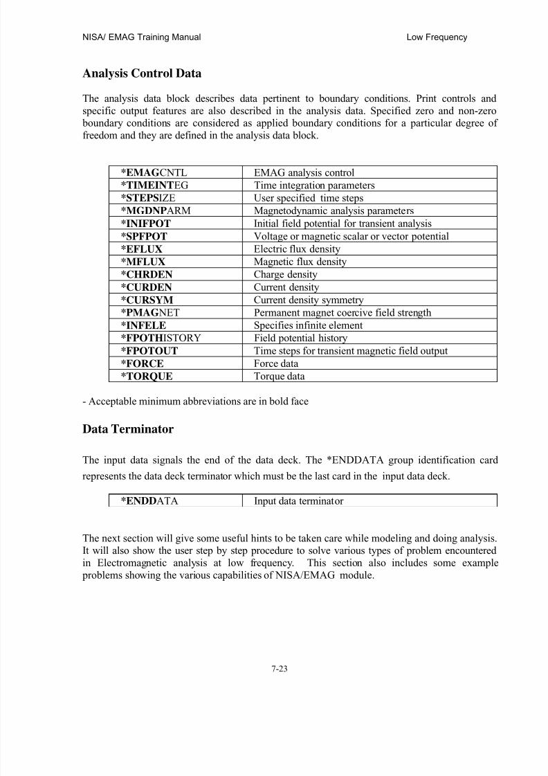
8/12/2019 emagtm
http://slidepdf.com/reader/full/emagtm 101/246
NISA/ EMAG Training Manual Low Frequency
7-23
Analysis Control Data
The analysis data block describes data pertinent to boundary conditions. Print controls andspecific output features are also described in the analysis data. Specified zero and non-zero boundary conditions are considered as applied boundary conditions for a particular degree of
freedom and they are defined in the analysis data block.
*EMAGCNTL EMAG analysis control*TIMEINTEG Time integration parameters*STEPSIZE User specified time steps*MGDNPARM Magnetodynamic analysis parameters*INIFPOT Initial field potential for transient analysis*SPFPOT Voltage or magnetic scalar or vector potential*EFLUX Electric flux density*MFLUX Magnetic flux density
*CHRDEN Charge density*CURDEN Current density*CURSYM Current density symmetry*PMAG NET Permanent magnet coercive field strength*INFELE Specifies infinite element*FPOTHISTORY Field potential history*FPOTOUT Time steps for transient magnetic field output*FORCE Force data*TORQUE Torque data
- Acceptable minimum abbreviations are in bold face
Data Terminator
The input data signals the end of the data deck. The *ENDDATA group identification card
represents the data deck terminator which must be the last card in the input data deck.
*ENDDATA Input data terminator
The next section will give some useful hints to be taken care while modeling and doing analysis.It will also show the user step by step procedure to solve various types of problem encounteredin Electromagnetic analysis at low frequency. This section also includes some example problems showing the various capabilities of NISA/EMAG module.

8/12/2019 emagtm
http://slidepdf.com/reader/full/emagtm 102/246
NISA/EMAG Training Manual Low Frequency
7-24
HINTS FOR USING NISA/EMAG
This chapter gives useful hints for running NISA/EMAG. Both modeling and analysis hints arediscussed in this chapter. Modeling hints give information that an EMAG user should knowabout DISPLAY III. The analysis hints cover the NISA/EMAG module itself. The analyses are
categorized based on type of analysis such as electrostatic analysis, steady current flow,magnetostatic etc.
MODELING HINTS
Your Electromagnetic Problem
The basic steps to be followed for solving your electromagnetic problem:
Use the steps below to solve your problem.
1. Define your electromagnetic problem.
2. Identify your problem region in two or three dimension space. If part of your problem possesses open geometry, then you have to choose the problem space depending onwhether you are using infinite elements or not.
a. If you are using all finite elements : Choose sufficiently large space for the problem sothat some of fields or their derivatives decay to zero or negligible at the problem boundary. These fields will depend on the type of problem. b. If you using infinite elements on the open boundary: Choose sufficient space so that
the open problem region is roughly 3-10 times the dimesions of the electromagneticsources.
3. Define the various materials in the problem and their material properties.
4. Identify which of the fields or their derivatives tend to zero at the problem boundary.
a. If you are using all finite elements: Put these boundary conditions on the finiteelements
b. If you using infinite elements on the open boundary: Identify the faces of theinfinite elements that tend to infinity.
Also identify all other boundary conditions in the problem. e.g. currents in coppercoils, charge on a capacitor plate etc. Define the correct locations of these boundaryconditions.
5. Identify the analysis type which will depend on the governing equation.
6. Choose any one but only one self-consistent system of units for all the quantities. e.g.MKS units

8/12/2019 emagtm
http://slidepdf.com/reader/full/emagtm 103/246
NISA/ EMAG Training Manual Low Frequency
7-25
7. Solve this governing equation subject to the defined material properties and boundaryconditions. The solution will yield the value of the fields mentioned in 4. Use thissolution to compute all other required quantities.
The basic steps to be followed for solving your electromagnetic problems by Finite Element
method :Use the steps below to solve your problem.1. Define your electromagnetic problem.2. Identify your problem region in two or three dimensional space. Choose sufficient
space as explained above.3. Define the various materials in the problem and their material properties.4. Identify all the boundary conditions as explained above.5. Identify the analysis type which will depend on the governing equation.6. Choose any one but only one self-consistent system of units for all the quantities. e.g.
MKS units.7. Subdivide the problem region into finite elements. During subdivision please note that
you have to put more number of elements in subregions where the spatial field variationis large and vice versa. Also the higher the number of elements you use the better theaccuracy you get. While subdivision you have to note that no element should definemore than one material, that is, the element face will always lie on the interface of twoor more materials. Thus the elements demarcate different materials. The creation ofelements automatically entails the creation of nodes depending on what type of elementyou are using. Defining the nodes means specifying the spatial position of all the nodesin the chosen coordinate system. Next define proper connectivity between the nodesand elements. Then your finite element mesh is fully defined.
8. Define the material properties of all the materials in the problem, that is, define theirnumerical values in the system of units you have chosen. Put these values for all theelements depending on what material they define.
9. Put the value of the relevant potentials equal to zero at the problem boundarydepending on how the problem is defined. Put these values on the boundary nodes or onthe face of the element that lies on the boundary. Again this will depend on the type offield mentioned above. For electric field analysis, the unspecified boundary willassume a homogeneous Neumann boundary, where, no flux/current can cross this boundary and for magnetic field analysis, any unspecified boundary will assume thetangential magnetic field along the boundary to be zero.
10. Put all the remaining boundary conditions at the correct spatial locations. Put thesevalues on the nodes or on the face of the element or on the whole element that definethe correct location for the boundary conditions. Again this will depend on the type of boundary condition defined above.
11. Define the analysis type identified earlier and solve the problem using the correct FiniteElement solver. The solution will yield the value of the fields mentioned in 4. Use thissolution to compute all other required quantities.
12. For more details on the Finite Element method, please consult any basic book on the
Finite Element method .

8/12/2019 emagtm
http://slidepdf.com/reader/full/emagtm 104/246
NISA/EMAG Training Manual Low Frequency
7-26
DISPLAY III : Post-Processing for EMAG
After you have run your EMAG solver two files are created :1. A post file > *26.dat as given above.2. A OUT file > *.out. The * corresponds to the filename you had given to your NIS
file by default or to some other name you had specified. This is an ASCII filewhich contains all your input finite element data and all results from EMAGsolver. You can edit this file for more processing or simply to get a hard copy.Read the post file in DISPLAY.
In the main menu you will see POST RESULTS. Select this. You will see the sub-menus. Theyare explained below:
1. CONTOURS : This menu is used to plot your EMAG results on the screen ascontours. Select this and you see the following sub-menus:
a. PICK RESULTS : This is to select a particular quantity from a list of quantities
that was produced as an output by the EMAG solver. b. CONTOUR STATUS : This is to set contour plotting parameters.
2. GRAPHS : This menu is used to plot your EMAG results in graphical form on thescreen or record them in files.
3. MISCELLANEOUS : In this menu select EMAG ARROW PLOTS. Then select therequired quantity to see it in the field plotting mode with directions of thefields shown by arrows.
HINTS REGARDING ELECTROMAGNETIC PROBLEM
The theoretical aspects of electromagnetic problems at low frequency are given at the beginning of this chapter. The practical approach for solving these problems is given below.
Electrostatic fields :
Electrostatic analysis :
In this the solution is found for the electrostatic scalar potential at the nodal locations in the problem region you have defined. It is important to note that you have to choose your
problem region properly as explained below.
i. Decide whether your problem is 2 or 3 dimensional. If the potential variation in onedirection is negligible or you are not interested in the potential variation in one particular direction then you can solve your problem in 2 D. If this does not hold thensolve your problem in 3 D. Also if your problem is axisymmetric the solve your problem in 2 D such that your 2 D coincides with the any plane passing through the tryaxis of symmetry.

8/12/2019 emagtm
http://slidepdf.com/reader/full/emagtm 105/246
NISA/ EMAG Training Manual Low Frequency
7-27
ii. Choose your problem region in 2 or 3 D space large enough such that the potentialvalue at the boundary of the problem is negligible or tends to zero as compared to itsmaximum value in the problem ( say 0.1 to 1 % ). There will be two cases:a. If you are using finite elements only: A simple thumb rule is that you locate the
boundary at about 5 to 50 times the maximum dimension of your source region. As
you get experience you will be able to apply your judgement. b. If you using infinite elements on the open boundary: Choose sufficient space so thatthe open problem region is roughly 3-10 times the dimension of the electromagneticsources.
iii. Identify whether there is any symmetry in the problem, that is, the lines which are perpendicular to the equipotential lines (which are the lines of symmetry). If these linesare regular and can be identified easily you can use the concept of symmetry, otherwisedon't use this concept. The Electric field is parallel to these lines and hence the normal
electric field or the derivative of the potential normal to these lines is zero.
After you have defined your problem region adequately, use the following steps:
1. Define the complete geometry you will use for your finite element model generationincluding the problem regions as defined above. As far as possible choose the exactgeometry of the actual problem. In some cases the geometry may be quite involved andconverting some of the geometry to simple shapes may not affect the solution: you canthen choose the simplified geometry. If the solution gets affected than do not go forsimplification and choose the actual geometry. Identify clearly all the materials thatdefine the geometry.
2. Use DISPLAY III to define your geometry using grids (points), lines, curves and primitive geometry entities if possible. Next you use them to create patches for 2 D andhyperpatches for 3 D problems. Note that the patches ( for 2 D ) or hyperpatches (
for 3 D ) should cover your entire geometry without overlapping. The only
exception to this is the portion where you want to create finite elements from
nodes. These patches or hyperpatches are a must for creating the finite element
mesh.3. In DISPLAY III use the patches or hyperpatches to create the finite elements. Assign
each element to the proper material. These elements should cover the entire geometrywithout any overlap. All adjacent elements should be connected to each other. For this
use
NODES -> NODE MANAGEMENT - > NODE MERGE.
To verify whether you have done this correctly use
VIEW -> DISPLAY -> BOUNDARY -> ALL ELEMENTS.
The display should show white lines only at the problem boundary. Any
intermediate white lines show that the conditions given above do not hold and you
have to check for the same.4. Enter your material properties, that is, the value of permittivity of the material. Use FE
MODEL DATA. For isotropic material enter the permittivity in EXX only and keepingEYY and EZZ blank. For anisotropic case enter the proper values in EXX, EYY andEZZ.
5. Enter the boundary conditions:

8/12/2019 emagtm
http://slidepdf.com/reader/full/emagtm 106/246
NISA/EMAG Training Manual Low Frequency
7-28
a. Identify all the portions of the problem boundary where the potential tends to zero.Use FE BOUNDARY CONDITIONS -> EMAG -> SFPPOT
to put the potential = 0 at those boundary nodes. b. At the remaining portion of the boundary the normal derivative of the potential is zero
or is specified ( see c.3 below). ∂φ/∂n = 0 is a natural boundary condition for the
finite element analysis. Hence you should not specify any boundary conditionfor nodes on these portions.
c. Identify all the other given boundary conditions in the problem viz : boundaryconditions due to sources. These will be in 3 forms;
1. The electrostatic potential is given -> use SFPPOT
2. The charge density is given -> use CHRDEN
3. The normal electric field is given at some portion of the problem boundary -> useEFLUX
6. Use NISA FORMS to define the analysis type, analysis data, the ouput file names andany print controls. For analysis type use EFIELD and SUBA = ESTAT.
7. Finally save your database, nisa and session files.
8. Run your nisa file in EMAG and get the solution.9. Use DISPLAY III to see the output POST files or an ordinary ASCII editor to see theOUT file.
10. The force or torque on a moving object can be computed by using FORCE orTORQUE option in NISA FORMS -> NISA DATA GROUP -> MFIELD.
Steady state current flow:
All the information given above applies except for the following differences:
1. The normal derivative of potential or the normal electric field will not be specified but
the normal current density is specified. Hence use the EFLUX option to enter thevalue of normal current density only. Note the current can be DC only.2. There will not be any charge density. Hence do not use the CHRDEN option.3. You can use Coupled Thermal analysis to obtain the temperature distribution.4. For analysis type use EFIELD and SUBA = SCFL.
Magnetostatic fields :
Magnetostatic analysis using magnetostatic vector potential A: In this the solution is found forthe magnetostatic vector potential at the nodal locations in the problem region you have defined.All the information given above applies except for the following differences:
1. Use magnetostatic vector potential A instead of electrostatic potential φ. 2. Use magnetic field intensity H instead of electric field E . 3. Use magnetic flux density B instead of electric flux density D. 4. Since ∇ × A = B, when the normal derivative of A is zero then B is perpendicular to
the line of symmetry. When normal derivative of A is not zero then the tangentialcomponent of B is specified at the boundary. For the other case use MFLUX to specifythe tangential component of B.

8/12/2019 emagtm
http://slidepdf.com/reader/full/emagtm 107/246
NISA/ EMAG Training Manual Low Frequency
7-29
5. Enter your material properties, that is, the value of permeability of the material. Use FE
MODEL DATA.a. For isotropic material enter the permeability in MUXX only and keeping MUYY and
MUZZ blank. For anisotropic case enter the proper values in MUXX, MUYY andMUZZ. Note : you have to enter the reciprocal of permeabilty.
b. For ferromagnetic materials use MUXX for entering any dummy value. Then click tothe right of MUXX and enter the B-H curve identification number. Next in NISA FORMS -> NISA DATA GROUP -> MFIELD click B-Htable and enter the H and B values.
c. For permanent magnets if the B-H table is specified then you have to find the value ofmagnetic coercivity from the B-H curve. This is the value of H at the point where thecurve cuts the B = 0 axis. You have to choose the absolute value of H. Then you shiftthe B-H curve to the right by the value of coercivity found above. Enter the B-H tableas in b. above. If B-H curve is not specified then you should know the value ofmagnetic coercivity. To enter the value of magnetic coercivity use PMAGNET option and specify Hcx, Hcy and Hcz in x , y and z directions. You have to specify
this for both the cases.
6. Enter the boundary conditions:a. Identify all the portions of the problem boundary where the magnetic potential tends to
zero. Use FE BOUNDARY CONDITIONS -> EMAG -> SFPPOT to put the potential = 0 at those boundary nodes, that is, Ax = Ay = Az = 0.
b. At the remaining portion of the boundary the tangential magnetic field zero or isspecified ( see c.3 below). This is a natural boundary condition for the finite elementanalysis. Hence you should not specify any boundary condition for nodes on
these portions.c. Identify all the other given boundary conditions in the problem viz : boundary
conditions due to sources. These will be in 4 forms ;1. The magnetostatic potential is given -> use SFPPOT
2. The current density is given -> use CURDEN
3. The tangential magnetic flux density is given at some portion of the problem boundary -> use MFLUX (for 2 D only)
3. The magnetic coercivity is given. Use the PMAGNET option as givenabove.
8. For analysis type use MFIELD andSUBA = MGSV for 2 D problems.
and SUBA = MGVP for 3 D problems.For problems with B-H curve (nonlinear) you have to specify the number of iterations,relaxation parameter etc. in NISA FORMS -> NISA DATA GROUP -> MFIELD.Then use the EMAGCNTRL option
9. The force or torque on a moving object can be computed by using FORCE orTORQUE option in NISA FORMS -> NISA DATA GROUP -> MFIELD.

8/12/2019 emagtm
http://slidepdf.com/reader/full/emagtm 108/246
NISA/EMAG Training Manual Low Frequency
7-30
Magnetostatic analysis using magnetostatic scalar potential φφφφ :
In this the solution is found for the magnetostatic scalar potential at the nodal locations in the problem region you have defined. All the information given above applies except for thefollowing differences:
1. Use magnetostatic scalar potential φm instead of magnetostatic potential A. 2. Since H = −−−− ∇ φ m , when the normal derivative of φ is zero then B is parallel to the
line of symmetry. When normal derivative of φm is not zero then the normalcomponent of B is specified at the boundary. For the case of ∂φ/∂n = 0 you need not putany boundary condition. For the other case the MFLUX option is not available.
3. For analysis type use MFIELD and SUBA = MGSS for 3 D problems only.For problems with B-H curve (nonlinear) you have to specify the number of
iterations, relaxation parameter etc. inNISA FORMS -> NISA DATA GROUP -> MFIELD. Then use the
EMAGCNTRL option
4. The force or torque on a moving object can be computed by using FORCE orTORQUE option in NISA FORMS -> NISA DATA GROUP -> MFIELD.
Magnetodynamic fields :
Magnetodynamic analysis for sinusoidal time varying currents or magnetic
fields using vector potential A :
In this the solution is found for the vector potential at the nodal locations in the problem region.At present the analysis is available in 2 D only and only the z or θ component of A is obtained.
All the information given above applies except for the following differences:
1. In CURDEN you have to specify the frequency and phase of the current2. You can change the value of frequency using MGDNPARM where you can specify
frequency, the output type ( polar or real/imaginery form ) and the chosen conductor.3. For analysis type use MFIELD and SUBA = MGDN for 2 D problems only.4. The solutions can be viewed at different electrical angles ( 0 to 360 degrees ). For this use
FPOTOUT in NISA FORMS -> NISA DATA GROUP -> MFIELD.
5. Permanent magnet capability is not applicable.
8/12/2019 emagtm
http://slidepdf.com/reader/full/emagtm 109/246
NISA/ EMAG Training Manual Low Frequency
7-31
Transient Magnetic analysis for arbitrary time varying currents or magnet fields
using vector potential A :
In this the solution is found for the vector potential at the nodal locations in the problem regionyou have defined. At present this analysis is available in 2 D only and therefore, only the z or θ
component of A canl be obtained. All the information given above applies except for thefollowing differences:
1. Permanent magnet capability is available.2. In CURDEN you have to specify the TIME AMPLITUDE identification number. Then
choose NISA FORMS -> NISA DATA GROUP -> MFIELD. Enter the values ofcurrent for various time instants in the TIME AMPLITUDE option.
3. You have to enter the time integration data parameters inNISA FORMS -> NISA DATA GROUP -> MFIELD. Then choose the optionTIMEINTEG or STEPSIZE.
4. The solutions can be viewed at different time instants. For this use FPOTOUT
NISA FORMS -> NISA DATA GROUP -> MFIELD.5. The force or torque on a moving object can be computed by using FORCE or TORQUE
option in NISA FORMS -> NISA DATA GROUP -> MFIELD.
6. For analysis type use MFIELD and SUBA = TMAG for 2 D problems only.
Coupled Electromagneto-Thermal analysis :
In this you can do a heat transfer analysis in electromagnetic devices due to the power losses produced by the presence of currents. This analysis can be carried out coupled with :
a. EFIELD -> SCFL b. MFIELD -> MGSV
-> MGVP
-> MGSS
-> MGDN
-> TMAG
For more details about the use of heat transfer analysis please refer to the HEAT Manual.For using HEAT analysis coupled with EMAG please note the following:
1. First model the EMAG problem and create the corresponding NISA file. In this NISAfile you add :
a. CHEAT = ON after SUBA = .... b. Put SAVE = 20,26 instead of SAVE = 26.
2. Use the same model and remove all the material properties and boundary conditions.Then add the material properties and boundary conditions for HEAT analysis. Changethe analysis type from EMAG to HEAT and also add all the required analysis parameters print controls etc. Create the corresponding NISA file. In this NISA file youadd: read, EMAGNISfilename20.dat after the boundary conditions.

8/12/2019 emagtm
http://slidepdf.com/reader/full/emagtm 110/246
NISA/EMAG Training Manual Low Frequency
7-32
3. For static analysis type use SHEAT4. For transient analysis type use THEAT5. Solutions are obtained for the temperature distribution only.

8/12/2019 emagtm
http://slidepdf.com/reader/full/emagtm 111/246
NISA/ EMAG Training Manual MODELING Session 1
8-1
CHAPTER 8
MODELING SESSION 1
A simple modeling session will be presented in this chapter. You will use the menu mode(mouse driven) to communicate with the program. This mode is easy to operate and requires noknowledge of the DISPLAY command syntax.
Although the menu mode is user friendly, describing the steps to be followed for such amodeling assignment is an enormous task. In this text, menu selections are described as a chainof commands and follow a set of conventions. It is very important to get used to theseconventions before attempting these sample sessions. The conventions adhered to are as follows :
a) Bold capital entries in shaded boxes are selections from the top level menu. b) Underlined entries in shaded boxes sre selections from the sublevel menu.
c) Ordinary capital in shaded boxes are selections from the operation menu (tokens).d) Italic capital entries in shaded double boxes are selections from the hot button menu.e) The symbol ‘→’ means clicking the left button of the mouse.f) The symbol ‘←’ means clicking the right button of the mouse.g) Entries in non shaded boxes mean inserting data from the keyboard or the numeric pad.h) The symbol <CR> is used to describe a carriage return.
Also, remember that the left mouse button (→) is used for accepting a certain operation and to proceed to the next level of operations. Clicking the right button of the mouse is generally doneat the end of one complete set of instructions to get out of that chain. Almost all the stepsdescribed in this tutorial, thus, end with the symbol ‘←’ to instruct that the right button of the
mouse be clicked to end that set of instructions. Please keep an eye open for these symbols. Thecomplete chain of menu instructions for a certain task is kept within border lines to identifythem.
If you commit an error during the modeling session, you may use the “UNDO’ hot button toundo the last command. ‘ESC’ on the keyboard will abort the current operation.
The goal of this session is to model a nonlinear inductor, as shown in Figure 8.0. Due tosymmetry of the problem only a quarter of the inductor is modeled in the global XY plane. Thecoil is excited with 2000 A/m2. The material property (reluctivity) of copper and steel are definedas follows :
Material = IsotropicMUXX (steel) = BH table is used, see table (.8.1)MUXX (copper) = 7.957 x 10+5 Hm –1
Since the geometry of this inductor model is in the XY plane therefore 2D planar element ischosen. NISA offers one of the most complete element libraries among commercial softwares,and a list of currently available elements can be found in the User’s manual.
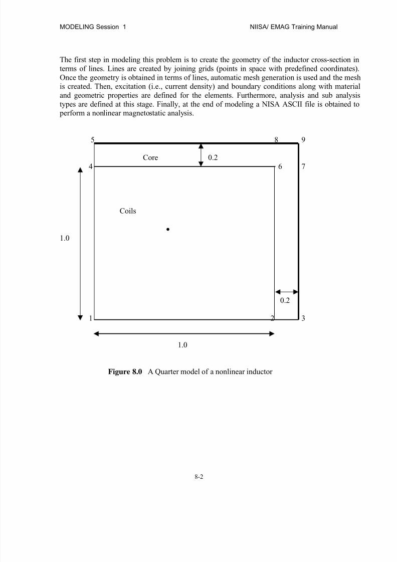
8/12/2019 emagtm
http://slidepdf.com/reader/full/emagtm 112/246
MODELING Session 1 NIISA/ EMAG Training Manual
8-2
The first step in modeling this problem is to create the geometry of the inductor cross-section interms of lines. Lines are created by joining grids (points in space with predefined coordinates).Once the geometry is obtained in terms of lines, automatic mesh generation is used and the meshis created. Then, excitation (i.e., current density) and boundary conditions along with material
and geometric properties are defined for the elements. Furthermore, analysis and sub analysistypes are defined at this stage. Finally, at the end of modeling a NISA ASCII file is obtained to perform a nonlinear magnetostatic analysis.
5 8 9
Core 0.24 6 7
Coils
• 1.0
0.2
1 2 3
1.0
Figure 8.0 A Quarter model of a nonlinear inductor

8/12/2019 emagtm
http://slidepdf.com/reader/full/emagtm 113/246
NISA/ EMAG Training Manual MODELING Session 1
8-3
Step 1 Now create grid points for the given geometry. Enter the coordinate (0/0/0) usingkeyboard and hit <CR>. The user will see grid no. 1 appearing on the screen.Similarly, repeat this operation for the following grids, i.e. 2, 3, 4, 5, 6, 7, 8 and 9
respectively. See Figure (8.1),
Figure 8.1 Grid Generation
GEOM GRID CREATE XYZ COORDINATE XYZ DATA
Figure 8.1 Grid generation

8/12/2019 emagtm
http://slidepdf.com/reader/full/emagtm 114/246
MODELING Session 1 NIISA/ EMAG Training Manual
8-4
Step 2 Now create lines by joining two grid points. Pick two grid points 1 and 2 using cursor.
User will see line no. 1 appearing on the screen. Repeat this Figure 8.2 is obtained.
User can skip this step and proceed directly to step 4 if user chooses to create patches by picking4 grid points.
GEOM LINE CREATE WORK PLANE 2 GRIDS
CURSOR PICK
Figure 8.2 Patch generation

8/12/2019 emagtm
http://slidepdf.com/reader/full/emagtm 115/246
NISA/ EMAG Training Manual MODELING Session 1
8-5
Step 3 To generate a patch follow the command sequences given below. Pick two lines tocreate a patch or pick four grid points to create a patch. In this example step 3 is skipped, hencegrid method is chosen for patch creation.
Now pick grid points 1, 2, 4 and 6, respectively with cursor, user will see patch #1 appearing onscreen. Similarly, pick grid points, 2, 3, 6 and 7 for patch 2, grid points 6, 7, 9 and 8 for patch 3and finally pick grid points 4, 6, 9 and 5 to create patch #4.
Step 4 To generate finite element mesh choose the following command sequence. In this problem quadrilateral elements (element type 102) are chosen. Also E1/E2 are definedas 5/5, which means a patch will be descretized with 25 elements 5 in each direction,see Figure 8.3. User must be careful when descretizing different patches asconnectivity of the nodal points should always exist in the model.
Now pick patches 1, 2, 3 and 4, respectively, to create finite elements in the model, see Figure8.3.
GEOM PATCH CREATE LINE METHOD 2 LINES
CURSOR PICK
GEOM PATCH CREATE GRID METHOD 4 GRIDS
CURSOR PICK
FE GENRATION MESH FEG OPTION QUADRILATERAL E!/E2
CURSOR PICKINPUT PATCH

8/12/2019 emagtm
http://slidepdf.com/reader/full/emagtm 116/246
MODELING Session 1 NIISA/ EMAG Training Manual
8-6
Once the finite element mesh is generated, user must delete all unreferenced nodes. Also usermust merge the inactive nodes. This is an important step, because if inactive nodes are present inthe FE model then the analysis results will not be correct.
Figure 8.3 Finite Elements
FE GENRATION MESH FEG OPTION QUADRILATERAL E!/E2
CURSOR PICKINPUT PATCH

8/12/2019 emagtm
http://slidepdf.com/reader/full/emagtm 117/246
NISA/ EMAG Training Manual MODELING Session 1
8-7
Step 5 Now user must define the material properties. In this nonlinear inductor problem twomaterials exist, they are copper and steel. For steel BH curve is accounted, see Table8.1, for copper reluctivity = 7.957 x 10+5 Hm-1 is used.
In order to define reluctivity of each material follow the command syntax (1), see forms shownin Figure 8.4 and 8.5a respectively. User will define the material constants depending on theanalysis types. For the nonlinear material, the user should enter 1.0 in the first column of MUXXand click on the adjacent tile. The form in Figure 8.5a will appear. At this stage the user mustenter the BH curve number under IDCURV.
(1)
OR
(1)
NISA DATA GROUP NISA FORMS MATERIALMFIELD
FE GENERATION FE MODEL DATA MATERIAL DATA
ADD Emag
FE GENRATION NODES NODE MANAGEMENT DELETE INACTIVE
ALL
FE GENRATION NODES NODE MANAGEMENT MERGE NODES
ALL
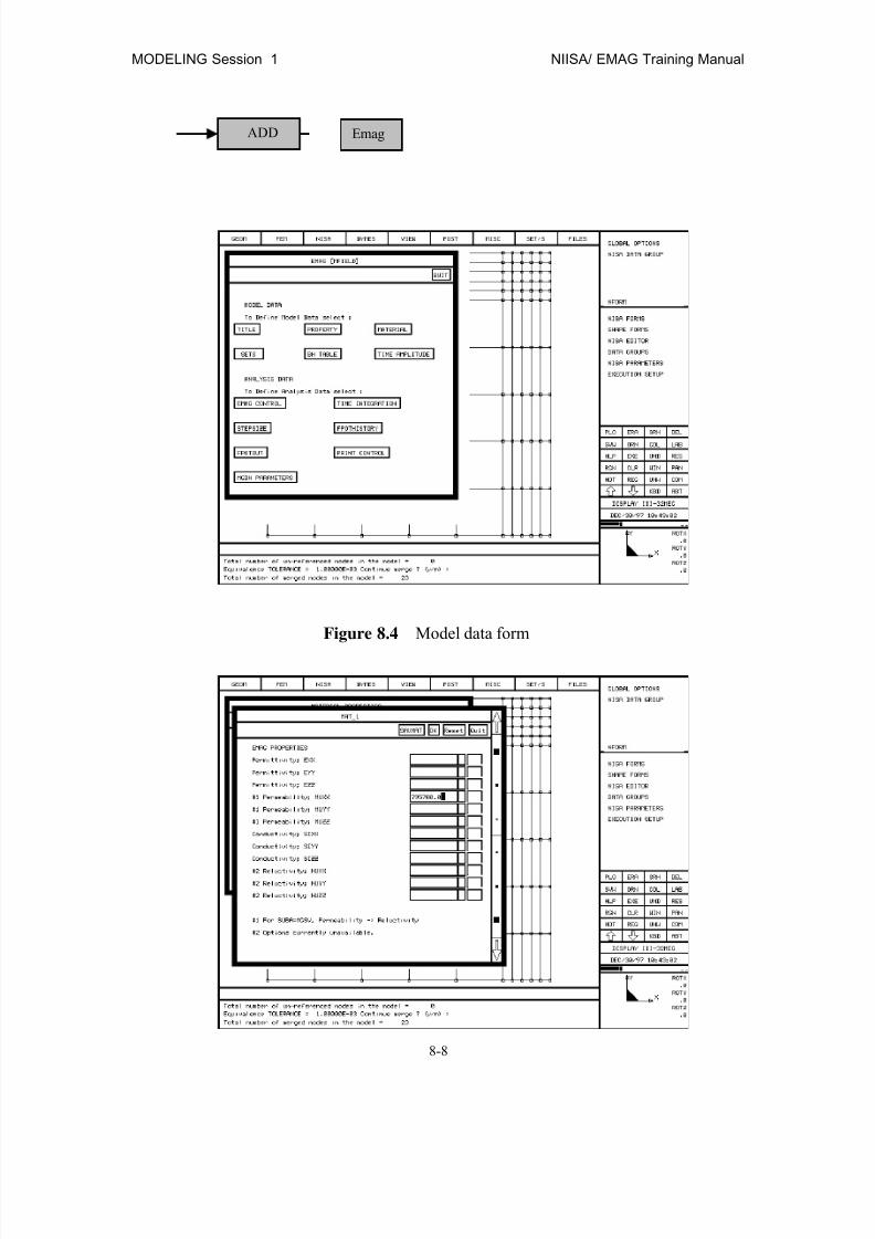
8/12/2019 emagtm
http://slidepdf.com/reader/full/emagtm 118/246
MODELING Session 1 NIISA/ EMAG Training Manual
8-8
Figure 8.4 Model data form
ADD Emag

8/12/2019 emagtm
http://slidepdf.com/reader/full/emagtm 119/246
NISA/ EMAG Training Manual MODELING Session 1
8-9
For nonlinear steel follow the command and sequence (2) and enter the BH table data’s in theform shown in Figure 7.6. The BH table used here is also given in table 1.
(2)
NISA DATA GROUP NISA FORMS BH TABLE
ADD
MFIELD
ENTER BH TABLE
Figure 8.5a Material property form
Figure 8.5b BH Curve ID form

8/12/2019 emagtm
http://slidepdf.com/reader/full/emagtm 120/246
MODELING Session 1 NIISA/ EMAG Training Manual
8-10
Table 8.1. BH Table
H B150.53 1.0154.41 1.025
158.33 1.05162.3 1.075166.33 1.1170.43 1.125174.65 1.25179.01 1.175183.55 1.2188.34 1.225
Figure 8.6 BH table form

8/12/2019 emagtm
http://slidepdf.com/reader/full/emagtm 121/246
NISA/ EMAG Training Manual MODELING Session 1
8-11
193.46 1.25199.03 1.275205.2 1.3212.18 1.325220.27 1.35
229.87 1.375241.53 1.4256.03 1.425274.45 1.45298.32 1.475329.79 1.5371.87 1.525428.89 1.55506.97 1.575614.92 1.6765.39 1.625976.66 1.651275.2 1.6751699.7 1.72306.6 1.7253178.9 1.754439.0 1.7756268.2 1.88936.8 1.82512848.0 1.8518607.0 1.875
27128.0 1.939793.0 1.92558704.0 1.9587072.0 1.975129826.0 2.0
Step 6 Now user can define the boundary conditions for the nonlinear inductor model. TheDirichlet boundary condition is defined on the two sides of the steel core of theinductor, as shown in Figure 8.7.
FE GENERATION BOUNDARY CONDN. SPFPOTEMAG
BORDER
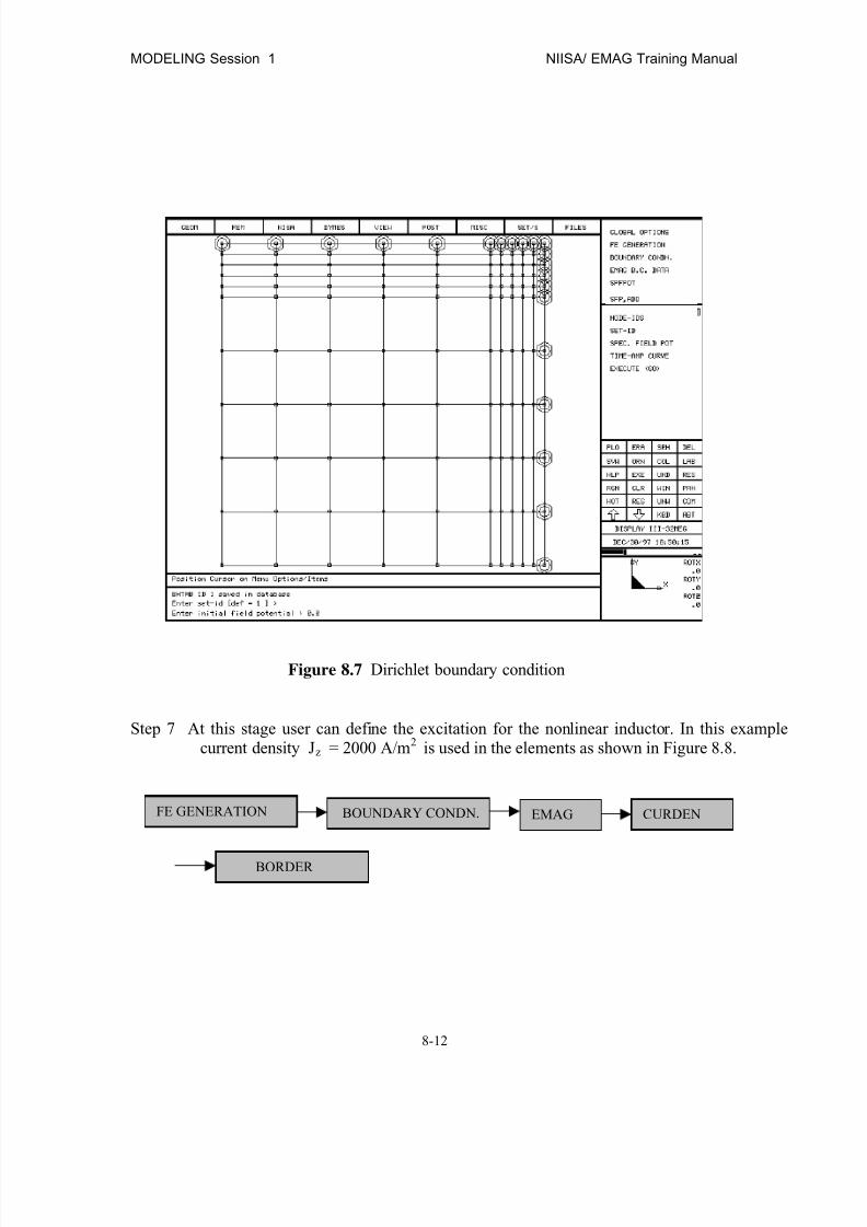
8/12/2019 emagtm
http://slidepdf.com/reader/full/emagtm 122/246
MODELING Session 1 NIISA/ EMAG Training Manual
8-12
Step 7 At this stage user can define the excitation for the nonlinear inductor. In this examplecurrent density Jz = 2000 A/m2 is used in the elements as shown in Figure 8.8.
FE GENERATION BOUNDARY CONDN. CURDENEMAG
BORDER
Figure 8.7 Dirichlet boundary condition

8/12/2019 emagtm
http://slidepdf.com/reader/full/emagtm 123/246
NISA/ EMAG Training Manual MODELING Session 1
8-13
Step 8 Finally, user must define the title, the EMAG control, and the executive command cardssuch as analysis type, and sub analysis type. The forms of which are shown in Figures8.9, 8.10 and 8.11 respectively. Follow the command sequences given below.
TITLE
EMAG CONTROL
Figure 8.8 Current density
NISA DATA GROUP NISA FORMS TITLEMFIELD
NISA DATA GROUP NISA FORMS EMAGCONTROL
MFIELD
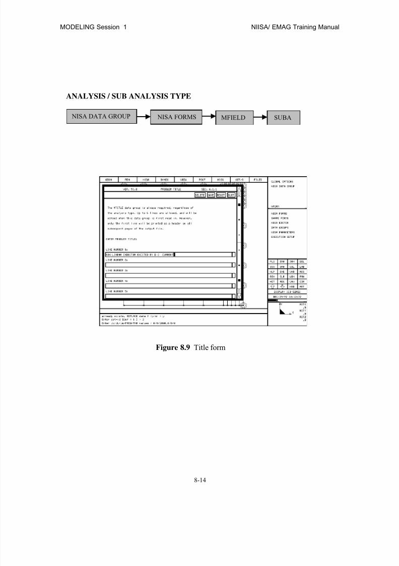
8/12/2019 emagtm
http://slidepdf.com/reader/full/emagtm 124/246
MODELING Session 1 NIISA/ EMAG Training Manual
8-14
ANALYSIS / SUB ANALYSIS TYPE
NISA DATA GROUP NISA FORMS SUBAMFIELD
Figure 8.9 Title form

8/12/2019 emagtm
http://slidepdf.com/reader/full/emagtm 125/246
NISA/ EMAG Training Manual MODELING Session 1
8-15
Figure 8.10 EMAG control form
Figure 8.11 Sub analysis form

8/12/2019 emagtm
http://slidepdf.com/reader/full/emagtm 126/246
MODELING Session 1 NIISA/ EMAG Training Manual
8-16
Step 9 The physical geometric properties are defined in this step. These properties aredependent on the type of element chosen. The nodal thicknesses are defined through entries inthe Element Property form shown in Figures 7.12 and 7.13
Step 10 After obtaining the finite element mesh of the problem, you have to check whether theelements are proper viz : warping, distortion, aspect ratio, connectivity etc. for thisfollow the menu sequence.
Step 11 Futhermore, user must write .NIS, .DBS and .NEU files. NISA input file will be usedfor running the EMAG analysis, whereas .DBS (binary file) and NEU (ASCII file)contains the geometry and the finite element information of the model. The files arewritten by the following the procedure given below
FE GENERATION →→→→ FE MODEL DATA →→→→ PROPERTY DATA →→→→
1) select ADD button in the ‘ELEMENT PROPERTIES’ form.
2) Select SHELL button in the ‘ELEMEMT TYPE’ form.
3) The form for inserting nodal thicknesses appears. Click the mouse button ‘→→→→’ tohighlight the box for Nodal Thickness 1. Insert the thickness value as 0.1.
4) Now click the box ‘ALL’ to repeat above thickness for all the nodes.
5) Click the ‘OK’ button to accept the defined values.
6) Now click the ‘QUIT’ button.
FILE MANAGEMENT →→→→ WRITE →→→→ NISA FILE →→→→ filename →→→→
FILE MANAGEMENT →→→→ WRITE →→→→ DATABASE FILE →→→→ filename →→→→
FILE MANAGEMENT →→→→ WRITE →→→→ NEUTRAL FILE →→→→ filename →→→→
You should enter the name of the file in which you want to store the above files.
FE GENERATION ELEMENTS. ELEMENT CHECKVERIFICATION
FE GENERATION ELEMENTS. NISA CHECKVERIFICATION

8/12/2019 emagtm
http://slidepdf.com/reader/full/emagtm 127/246
NISA/ EMAG Training Manual MODELING Session 1
8-17
Figure 8.12 Property forms
Figure 8.13 Property forms
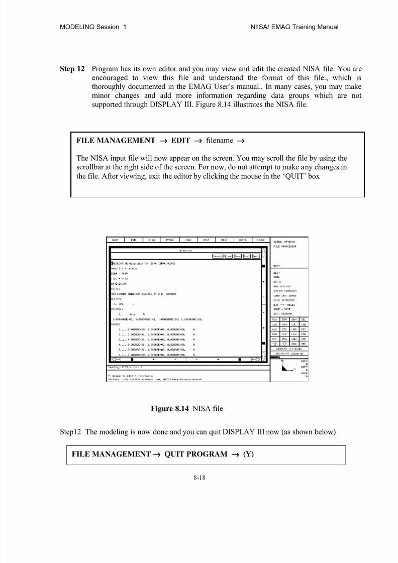
8/12/2019 emagtm
http://slidepdf.com/reader/full/emagtm 128/246
MODELING Session 1 NIISA/ EMAG Training Manual
8-18
Step 12 Program has its own editor and you may view and edit the created NISA file. You areencouraged to view this file and understand the format of this file., which isthoroughly documented in the EMAG User’s manual.. In many cases, you may make
minor changes and add more information regarding data groups which are notsupported through DISPLAY III. Figure 8.14 illustrates the NISA file.
Step12 The modeling is now done and you can quit DISPLAY III now (as shown below)
FILE MANAGEMENT →→→→ EDIT →→→→ filename →→→→
The NISA input file will now appear on the screen. You may scroll the file by using thescrollbar at the right side of the screen. For now, do not attempt to make any changes inthe file. After viewing, exit the editor by clicking the mouse in the ‘QUIT’ box
Figure 8.14 NISA file
FILE MANAGEMENT→→→→ QUIT PROGRAM →→→→ (Y)

8/12/2019 emagtm
http://slidepdf.com/reader/full/emagtm 129/246
NISA/ EMAG Training Manual MODELING Session 1
8-19
This completes modeling of the demonstration problem.
RUNNING EMAG CODE :
The next step is to run the analysis using EMAG. On workstations, user can type EMAG at prompt to run EMAG analysis. Whereas on PC choose option N in NISA386 menu OR executeEMAG through WINDOWS 95 if your version is WINDOWS based. Type the NISA input filename you had chosen earlier and hit <CR> to use the same file name as the output file.
POST PROCESSING : For viewing the results after a successful run of EMAG analysis followthe procedure below :
1)
2)
Now user will see the form which contains the output parameters to be post processed, seeFigure 8.15.
In this example we have chosen the Resultant Flux density (B) to be viewed. Figure 8.16 showsthe contour lines of the Magnetic Flux density distribution.
FILE MANAGEMENT READ POST FILES
POST RESULTS CONTOURS PICK RESULTS

8/12/2019 emagtm
http://slidepdf.com/reader/full/emagtm 130/246
MODELING Session 1 NIISA/ EMAG Training Manual
8-20
Figure 8.15 Output Parameters
Figure 8.16 Magnetic Flux density distribution in a nonlinear inductor
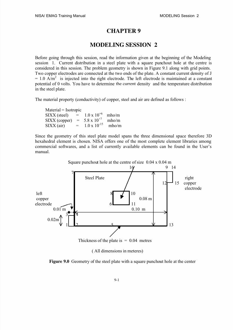
8/12/2019 emagtm
http://slidepdf.com/reader/full/emagtm 131/246
NISA/ EMAG Training Manual MODELING Session 2
9-1
CHAPTER 9
MODELING SESSION 2
Before going through this session, read the information given at the beginning of the Modelingsession 1. Current distribution in a steel plate with a square punchout hole at the centre isconsidered in this session. The problem geometry is shown in Figure 9.1 along with grid points.Two copper electrodes are connected at the two ends of the plate. A constant current density of J= 1.0 A/m2 is injected into the right electrode. The left electrode is maintained at a constant potential of 0 volts. You have to determine the current density and the temperature distributionin the steel plate.
The material property (conductivity) of copper, steel and air are defined as follows :
Material = Isotropic
SIXX (steel) = 1.0 x 10+6
mho/mSIXX (copper) = 5.8 x 10+7 mho/m
SIXX (air) = 1.0 x 10⁻¹⁵ mho/m
Since the geometry of this steel plate model spans the three dimensional space therefore 3Dhexahedral element is chosen. NISA offers one of the most complete element libraries amongcommercial softwares, and a list of currently available elements can be found in the User’smanual.
Square punchout hole at the centre of size 0.04 x 0.04 m16 9 14
7Steel Plate right
12 15 copperelectrode
left 8 10copper 0.08 melectrode 6 11
0.01 m 0.10 m3 4
0.02m1 2 2 5 13
Thickness of the plate is = 0.04 metres
( All dimensions in meteres)
Figure 9.0 Geometry of the steel plate with a square punchout hole at the center

8/12/2019 emagtm
http://slidepdf.com/reader/full/emagtm 132/246
MODELING Session 2 NIISA/ EMAG Training Manual
9-2
The first step in modeling this problem is to create the problem geometry. The lines are created by joining grids (points in space with predefined coordinates). These lines are used to createsurfaces called patches. These surfaces are used to create volumes called hyperpatches in such a
way that the full model is spanned. Once the geometry is obtained in terms of hyperpatches,automatic mesh generation is used to create the 3D mesh. Then, excitation (i.e., current densityand applied voltage) and the boundary conditions along with material and geometric propertiesare defined for the elements. Furthermore, analysis and sub analysis types are defined at thisstage. Finally, at the end of modeling a NISA ASCII file is obtained to perform a steady statecurrent flow analysis.
Step 1 Now create grid points for the given geometry. Enter the coordinate (-0.06/-0.04/-0.02)using keyboard and hit <CR>. The user will see grid no. 1 appearing on the screen.Similarly, repeat this operation for the following grids, i.e. 2, through 16 respectively.The grids are marked in Figure (9.0). The grids appear as in Figure (9.1).
Figure 9.1 Grid generation
GEOM GRID CREATE XYZ COORDINATE XYZ DATA

8/12/2019 emagtm
http://slidepdf.com/reader/full/emagtm 133/246
NISA/ EMAG Training Manual MODELING Session 2
9-3
Step 2 Now create lines by joining two grid points. Pick two grid points 1 and 2 using cursor.User will see line no. 1 appearing on the screen. Repeat this Figure 9.2 is obtained.
Figure 9.2 Generation of lines
Step 3 To generate a patch follow these command sequences. Pick two lines to create a patch or pick four grid points to create a patch. In this example patches are created using twolines. This is shown in Figure 9.3. For example Patch #1 is created using line nos # 1and 2.
GEOM LINE CREATE WORK PLANE 2 GRIDS
CURSOR PICK
GEOM PATCH CREATE LINE METHOD 2 LINES
CURSOR PICK
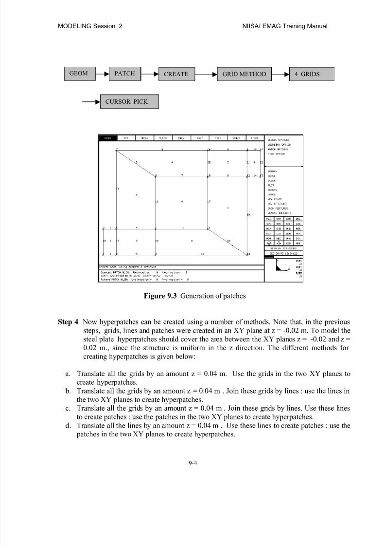
8/12/2019 emagtm
http://slidepdf.com/reader/full/emagtm 134/246
MODELING Session 2 NIISA/ EMAG Training Manual
9-4
Figure 9.3 Generation of patches
Step 4 Now hyperpatches can be created using a number of methods. Note that, in the previoussteps, grids, lines and patches were created in an XY plane at z = -0.02 m. To model thesteel plate hyperpatches should cover the area between the XY planes z = -0.02 and z =0.02 m., since the structure is uniform in the z direction. The different methods forcreating hyperpatches is given below:
a. Translate all the grids by an amount z = 0.04 m. Use the grids in the two XY planes to
create hyperpatches. b. Translate all the grids by an amount z = 0.04 m . Join these grids by lines : use the lines in
the two XY planes to create hyperpatches.c. Translate all the grids by an amount z = 0.04 m . Join these grids by lines. Use these lines
to create patches : use the patches in the two XY planes to create hyperpatches.d. Translate all the lines by an amount z = 0.04 m . Use these lines to create patches : use the
patches in the two XY planes to create hyperpatches.
GEOM PATCH CREATE GRID METHOD 4 GRIDS
CURSOR PICK
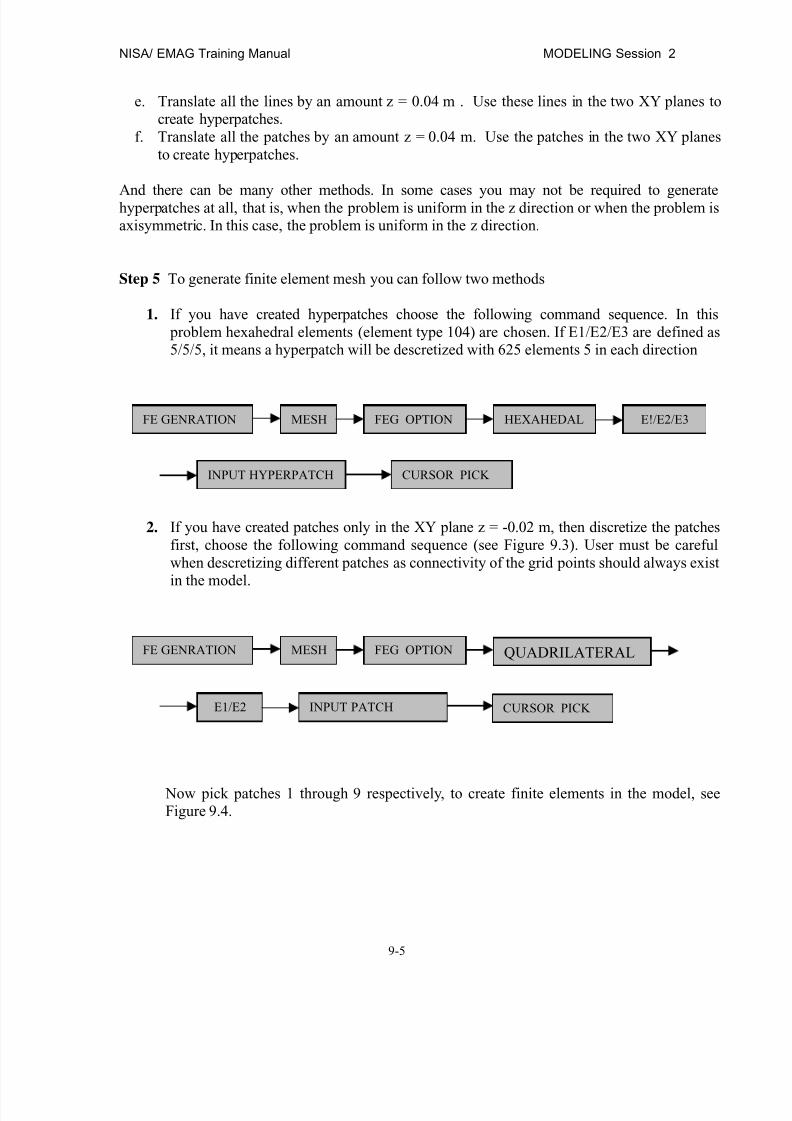
8/12/2019 emagtm
http://slidepdf.com/reader/full/emagtm 135/246
NISA/ EMAG Training Manual MODELING Session 2
9-5
e. Translate all the lines by an amount z = 0.04 m . Use these lines in the two XY planes tocreate hyperpatches.
f. Translate all the patches by an amount z = 0.04 m. Use the patches in the two XY planesto create hyperpatches.
And there can be many other methods. In some cases you may not be required to generatehyperpatches at all, that is, when the problem is uniform in the z direction or when the problem isaxisymmetric. In this case, the problem is uniform in the z direction.
Step 5 To generate finite element mesh you can follow two methods
1. If you have created hyperpatches choose the following command sequence. In this problem hexahedral elements (element type 104) are chosen. If E1/E2/E3 are defined as5/5/5, it means a hyperpatch will be descretized with 625 elements 5 in each direction
2. If you have created patches only in the XY plane z = -0.02 m, then discretize the patchesfirst, choose the following command sequence (see Figure 9.3). User must be carefulwhen descretizing different patches as connectivity of the grid points should always existin the model.
Now pick patches 1 through 9 respectively, to create finite elements in the model, seeFigure 9.4.
FE GENRATION MESH FEG OPTION HEXAHEDAL E!/E2/E3
CURSOR PICKINPUT HYPERPATCH
FE GENRATION MESH FEG OPTION QUADRILATERAL
E1/E2 CURSOR PICKINPUT PATCH
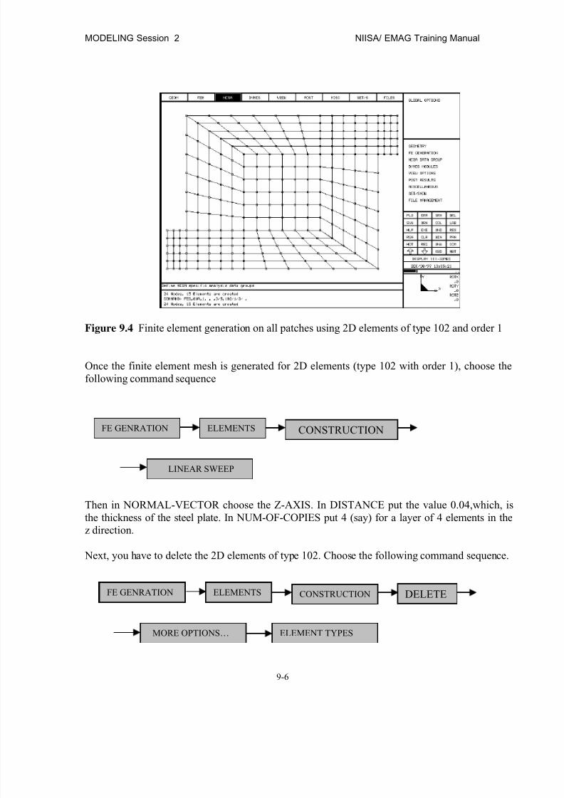
8/12/2019 emagtm
http://slidepdf.com/reader/full/emagtm 136/246
MODELING Session 2 NIISA/ EMAG Training Manual
9-6
Figure 9.4 Finite element generation on all patches using 2D elements of type 102 and order 1
Once the finite element mesh is generated for 2D elements (type 102 with order 1), choose thefollowing command sequence
Then in NORMAL-VECTOR choose the Z-AXIS. In DISTANCE put the value 0.04,which, isthe thickness of the steel plate. In NUM-OF-COPIES put 4 (say) for a layer of 4 elements in thez direction.
Next, you have to delete the 2D elements of type 102. Choose the following command sequence.
FE GENRATION ELEMENTS CONSTRUCTION
LINEAR SWEEP
FE GENRATION ELEMENTS CONSTRUCTION DELETE
MORE OPTIONS… ELEMENT TYPES

8/12/2019 emagtm
http://slidepdf.com/reader/full/emagtm 137/246
NISA/ EMAG Training Manual MODELING Session 2
9-7
Enter 102 for the ELEMENT TYPES.
Step 6 Once the finite element mesh is generated, user must delete all unreferenced nodes. Alsouser must merge the inactive nodes. This is an important step, because if inactive nodesare present in the FE model then the analysis results will not be correct. The final result
is shown in Figure 9.5.
Figure 9.5 The finite element mesh with element type 104 and order 1
FE GENRATION NODES NODE MANAGEMENT DELETE INACTIVE
ALL
FE GENRATION NODES NODE MANAGEMENT MERGE NODES
ALL

8/12/2019 emagtm
http://slidepdf.com/reader/full/emagtm 138/246
MODELING Session 2 NIISA/ EMAG Training Manual
9-8
Step 7 Now user must define the material properties. In this steel plate problem three materialsexist, they are copper, steel and air. For steel conductivity = 1.0 x 10+6 mho/m,, forcopper conductivity = 5.8 x 10+7 mho/m and for air conductivity = 1.0 x 10⁻¹⁵ mho/m.
In order to define conductivity of each material follow the command syntax (1), see formsshown in Figure 9.6a and 9.6b respectively. User will define the material constants depending onthe analysis types. For the steel plate, copper electrode and air, the user should enter therespective values in the first column of SIXX .
(1)
OR
(1)
NISA DATA GROUP NISA FORMS MATERIALMFIELD
FE GENERATION FE MODEL DATA
ADD
MATERIAL DATA
ADD Emag
Emag
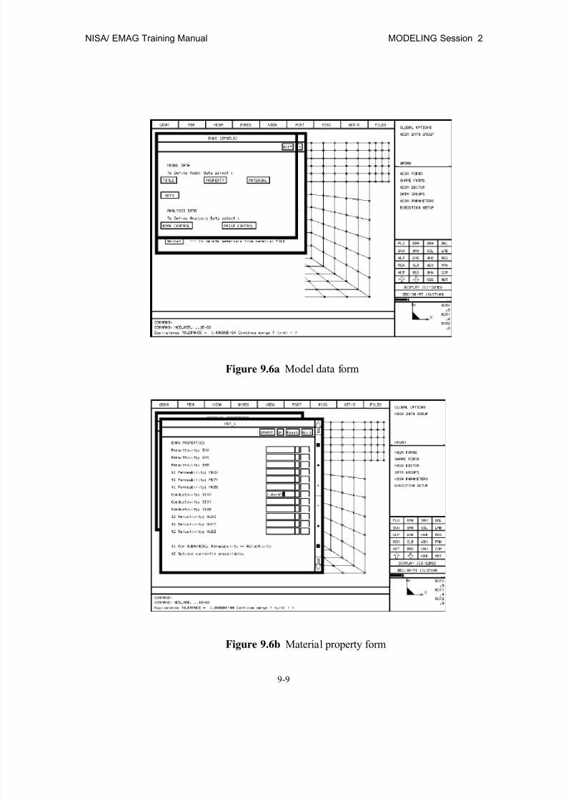
8/12/2019 emagtm
http://slidepdf.com/reader/full/emagtm 139/246
NISA/ EMAG Training Manual MODELING Session 2
9-9
Figure 9.6a Model data form
Figure 9.6b Material property form

8/12/2019 emagtm
http://slidepdf.com/reader/full/emagtm 140/246

8/12/2019 emagtm
http://slidepdf.com/reader/full/emagtm 141/246
NISA/ EMAG Training Manual MODELING Session 2
9-11
Now, the user should do the following : in SET-ID , the set id number should be entered 2 (say),in FACE-NUMBER the value 5 should be entered, in FLUX RATE the value 1.0 should beentered and in ELEMENT-IDS choose BOX CORNER and select the required elements. Theuser can find the face number 5 by the following command sequence
Now cursor pick an element on the right edge of the right copper electrode.
Figure 9.8 The injected current density on the right copper electrode
Step 10 Finally, user must define the title, the EMAG control, and the executive command cardssuch as analysis type, and sub analysis type. The forms of which are shown in Figures9.9, 9.10 and 9.11 respectively. Follow the command sequences given below.
FE GENERATION BOUNDARY CONDN. CURDENEMAG
ADD ON ELEMENTS
HOT FAC CURSOR PICK

8/12/2019 emagtm
http://slidepdf.com/reader/full/emagtm 142/246
MODELING Session 2 NIISA/ EMAG Training Manual
9-12
TITLE
EMAG CONTROL
ANALYSIS / SUB ANALYSIS TYPE
Figure 9.9 Title form
NISA DATA GROUP NISA FORMS TITLEEFIELD
NISA DATA GROUP NISA FORMS EMAG CONTROLEFIELD
NISA DATA GROUP NISA FORMS EXECUTIVE
SUBA
EFIELD

8/12/2019 emagtm
http://slidepdf.com/reader/full/emagtm 143/246
NISA/ EMAG Training Manual MODELING Session 2
9-13
Figure 9.10 EMAG control form
Figure 9.11 SUB analysis form

8/12/2019 emagtm
http://slidepdf.com/reader/full/emagtm 144/246
MODELING Session 2 NIISA/ EMAG Training Manual
9-14
Step 11 After obtaining the finite element mesh of the problem, you have to check whether theelements are proper viz : warping, distortion, aspect ratio, connectivity etc. for thisfollow the menu sequence.
Step 12 Futhermore, user must write .NIS, .DBS and .NEU files. NISA input file will be usedfor running the EMAG analysis, whereas .DBS (binary file) and NEU (ASCII file)contains the geometry and the finite element information of the model. These files arewritten by the following the procedure given below
Step 13 The program has its own editor and you may view and edit the created NISA file. Youare encouraged to view this file and understand the format of this file, which isthoroughly documented in the EMAG User’s manual. In many cases, you may makeminor changes and add more information regarding data groups which are notsupported through DISPLAY III. Figure 9.12 illustrates the NISA file.
FILE MANAGEMENT →→→→ EDIT →→→→ filename →→→→
The NISA input file will now appear on the screen. You may scroll the file by using thescrollbar at the right side of the screen. For now, do not attempt to make any changes inthe file. After viewing, exit the editor by clicking the mouse in the ‘QUIT’ box
FILE MANAGEMENT →→→→ WRITE →→→→ NISA FILE→→→→ filename →→→→ FILE MANAGEMENT →→→→ WRITE →→→→ DATABASE FILE→→→→ filename →→→→
FILE MANAGEMENT →→→→ WRITE →→→→ NEUTRAL FILE→→→→ filename →→→→
You should enter the name of the file in which you want to store the above files
FE GENERATION ELEMENTS. ELEMENT CHECKVERIFICATION
FE GENERATION ELEMENTS. NISA CHECKVERIFICATION
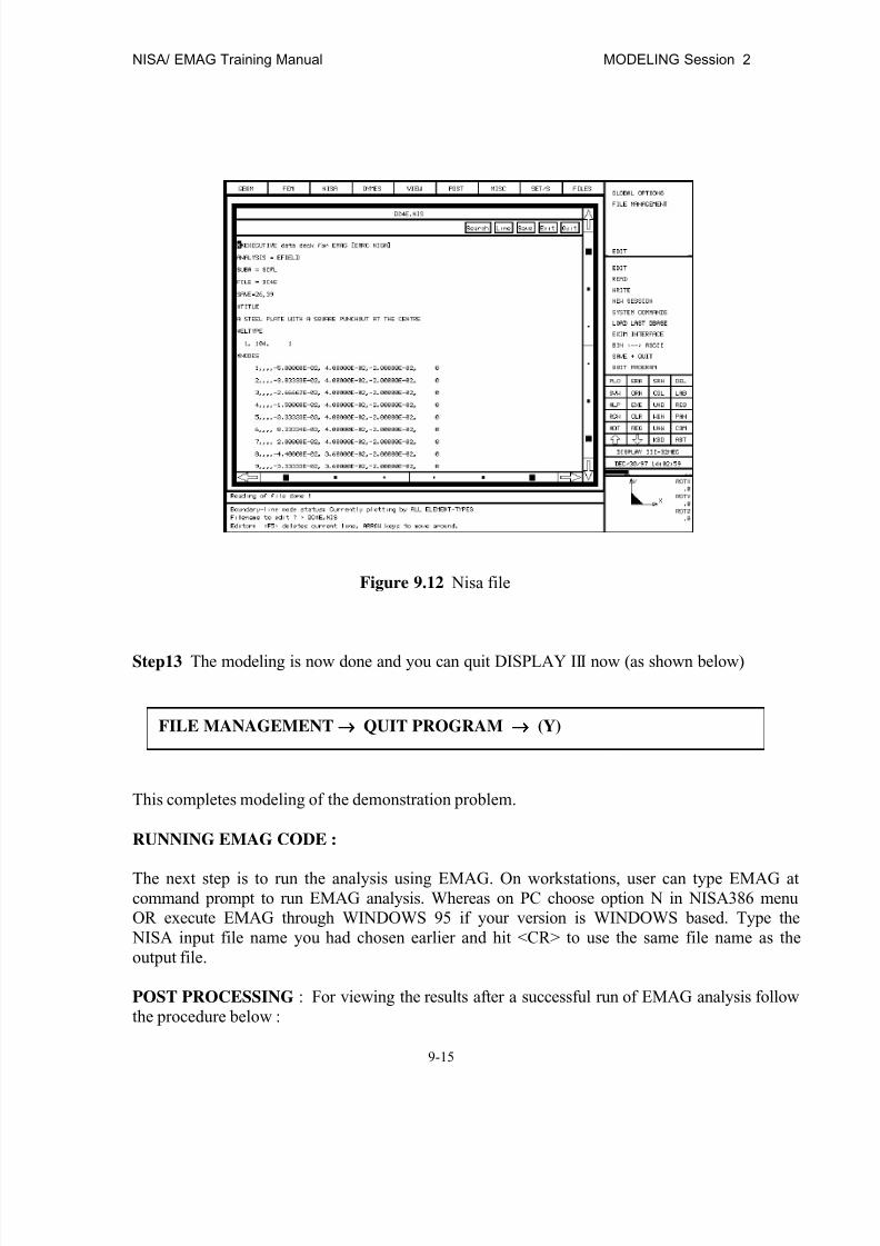
8/12/2019 emagtm
http://slidepdf.com/reader/full/emagtm 145/246
NISA/ EMAG Training Manual MODELING Session 2
9-15
Figure 9.12 Nisa file
Step13 The modeling is now done and you can quit DISPLAY III now (as shown below)
This completes modeling of the demonstration problem.
RUNNING EMAG CODE :
The next step is to run the analysis using EMAG. On workstations, user can type EMAG atcommand prompt to run EMAG analysis. Whereas on PC choose option N in NISA386 menuOR execute EMAG through WINDOWS 95 if your version is WINDOWS based. Type the NISA input file name you had chosen earlier and hit <CR> to use the same file name as theoutput file.
POST PROCESSING : For viewing the results after a successful run of EMAG analysis followthe procedure below :
FILE MANAGEMENT→→→→ QUIT PROGRAM →→→→ (Y)
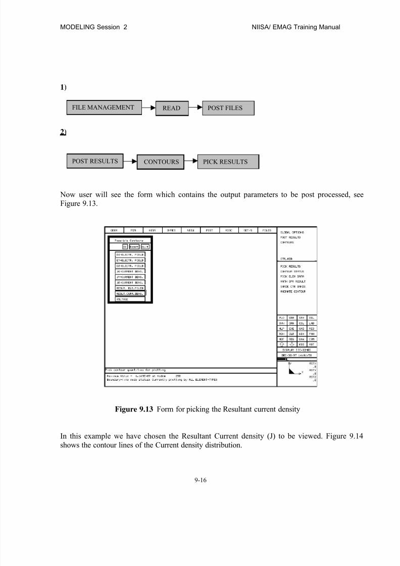
8/12/2019 emagtm
http://slidepdf.com/reader/full/emagtm 146/246
MODELING Session 2 NIISA/ EMAG Training Manual
9-16
1)
2)
Now user will see the form which contains the output parameters to be post processed, seeFigure 9.13.
Figure 9.13 Form for picking the Resultant current density
In this example we have chosen the Resultant Current density (J) to be viewed. Figure 9.14shows the contour lines of the Current density distribution.
FILE MANAGEMENT READ POST FILES
POST RESULTS CONTOURS PICK RESULTS

8/12/2019 emagtm
http://slidepdf.com/reader/full/emagtm 147/246
NISA/ EMAG Training Manual MODELING Session 2
9-17
Figure 9.14 The distribution of the Resultant current density
You can see the resultant current density field arrow plots using the following commandsequence. This is shown in Figure 9.15
POST RESULTS MISC. RESULTS EMAG ARROW PLOTS
CURRENT DENSITY
VIEW DISPLAY OPTIONS BOUNDARY LINE
ALL ELEMENTS

8/12/2019 emagtm
http://slidepdf.com/reader/full/emagtm 148/246
MODELING Session 2 NIISA/ EMAG Training Manual
9-18
Figure 9.15 The arrow field plot for the Resultant current density

8/12/2019 emagtm
http://slidepdf.com/reader/full/emagtm 149/246
NISA/ EMAG Training Manual MODELING Session 3
10-1
CHAPTER 10
MODELING SESSION 3
Before going through this session, read the information given at the beginning of the Modelingsession 1. The problem of a very long (can be considered infinite) parallel conducting plate ofnegligible thickness forming a capacitor is considered. The problem geometry is shown inFigure 10.0a. The voltage of the upper plate is assumed to be 100 volts and that of the lower plate to be –100 volts. You have to determine the electric field and the voltage distribution in themedium surrounding the two plates.
Upper conducting plate
100 volts
Lower conducting plate0.01 m
-100 volts
0.01The plates are very thin and are very long as shown by wavy lines
( All dimensions in meters )
Figure 10.0a Parallel plate capacitor
The material property (permittivity) of the air medium surrounding the two conducting plates isdefined as follows :
Material = Isotropic
EXX (air) = 8.85 x 10⁻¹²
F/m
The parallel conducting plates are very long in the direction perpendicular to this page. Hence,only a 2D model of the problem is necessary. This 2D model is taken in the XY plane. The platesare taken parallel to the X-axis and are centred with respect to the origin. Due to odd symmetryabout the X-axis, the potential φ on the X-axis is 0 volts. Due to even symmetry about the Y axisthe voltage φ is a mirror image of itself with respect to the Y axis. Hence, on the Y-axis theelectric field is tangential to it( i.e. x component is zero). Hence, only one fourth of the 2D
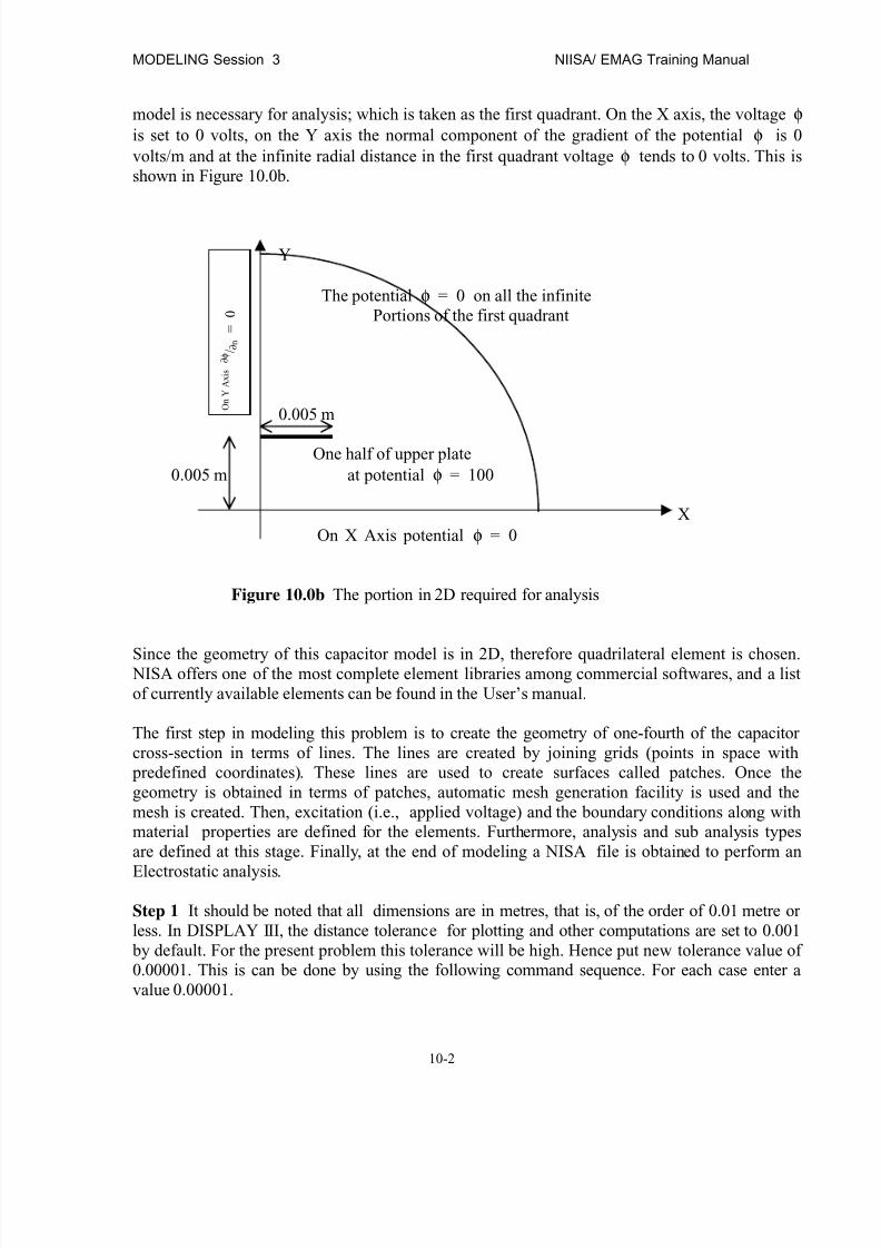
8/12/2019 emagtm
http://slidepdf.com/reader/full/emagtm 150/246
MODELING Session 3 NIISA/ EMAG Training Manual
10-2
model is necessary for analysis; which is taken as the first quadrant. On the X axis, the voltage φ is set to 0 volts, on the Y axis the normal component of the gradient of the potential φ is 0volts/m and at the infinite radial distance in the first quadrant voltage φ tends to 0 volts. This isshown in Figure 10.0b.
Y
The potential φ = 0 on all the infinitePortions of the first quadrant
0.005 m
One half of upper plate0.005 m at potential φ = 100
XOn X Axis potential φ = 0
Figure 10.0b The portion in 2D required for analysis
Since the geometry of this capacitor model is in 2D, therefore quadrilateral element is chosen. NISA offers one of the most complete element libraries among commercial softwares, and a listof currently available elements can be found in the User’s manual.
The first step in modeling this problem is to create the geometry of one-fourth of the capacitorcross-section in terms of lines. The lines are created by joining grids (points in space with predefined coordinates). These lines are used to create surfaces called patches. Once thegeometry is obtained in terms of patches, automatic mesh generation facility is used and themesh is created. Then, excitation (i.e., applied voltage) and the boundary conditions along withmaterial properties are defined for the elements. Furthermore, analysis and sub analysis typesare defined at this stage. Finally, at the end of modeling a NISA file is obtained to perform an
Electrostatic analysis.
Step 1 It should be noted that all dimensions are in metres, that is, of the order of 0.01 metre orless. In DISPLAY III, the distance tolerance for plotting and other computations are set to 0.001 by default. For the present problem this tolerance will be high. Hence put new tolerance value of0.00001. This is can be done by using the following command sequence. For each case enter avalue 0.00001.
O n Y A x i s
∂ φ / ∂ n
= 0
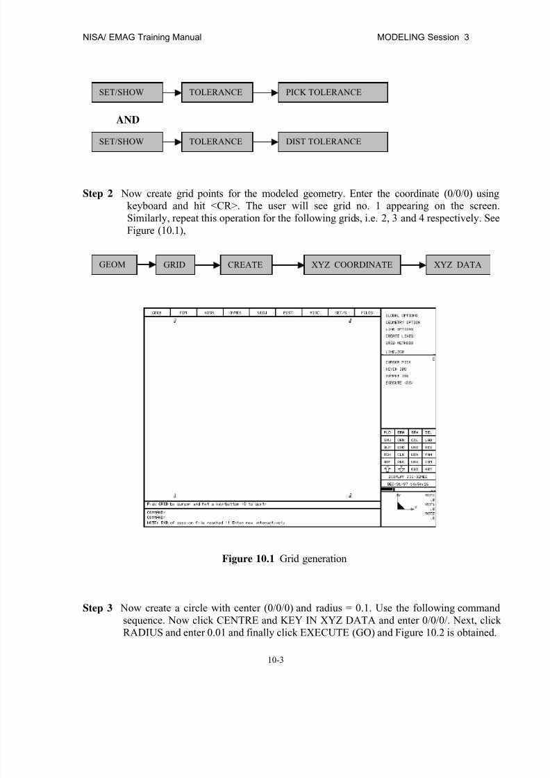
8/12/2019 emagtm
http://slidepdf.com/reader/full/emagtm 151/246
NISA/ EMAG Training Manual MODELING Session 3
10-3
AND
Step 2 Now create grid points for the modeled geometry. Enter the coordinate (0/0/0) usingkeyboard and hit <CR>. The user will see grid no. 1 appearing on the screen.Similarly, repeat this operation for the following grids, i.e. 2, 3 and 4 respectively. SeeFigure (10.1),
Figure 10.1 Grid generation
Step 3 Now create a circle with center (0/0/0) and radius = 0.1. Use the following commandsequence. Now click CENTRE and KEY IN XYZ DATA and enter 0/0/0/. Next, clickRADIUS and enter 0.01 and finally click EXECUTE (GO) and Figure 10.2 is obtained.
GEOM GRID CREATE XYZ COORDINATE XYZ DATA
SET/SHOW TOLERANCE PICK TOLERANCE
SET/SHOW TOLERANCE DIST TOLERANCE

8/12/2019 emagtm
http://slidepdf.com/reader/full/emagtm 152/246

8/12/2019 emagtm
http://slidepdf.com/reader/full/emagtm 153/246
NISA/ EMAG Training Manual MODELING Session 3
10-5
(2)
Figure 10.3 Generation of lines
Delete the lines numbered 6 through 11 using the command sequence (3) given below.
(3)
2 GRIDS CURSOR PICK
GEOMETRY LINE CREATE ON PRIM. CIRCLE
DELETE ENTITY-SETS LIN BORDEREXIT

8/12/2019 emagtm
http://slidepdf.com/reader/full/emagtm 154/246
MODELING Session 3 NIISA/ EMAG Training Manual
10-6
Figure 10.4 Deletion of lines
Step 5 To generate a patch follow the following command sequences. Pick two lines to create a patch. In this example patches are created using two lines. This is shown in Figure 9.3.For example Patch #1 is created using line nos # 5 and 2.
GEOM PATCH CREATE LINE METHOD 2 LINES
CURSOR PICK
GEOM PATCH CREATE GRID METHOD 4 GRIDS
CURSOR PICK

8/12/2019 emagtm
http://slidepdf.com/reader/full/emagtm 155/246
NISA/ EMAG Training Manual MODELING Session 3
10-7
Figure 10.5 Generation of patches
Step 6 To generate finite element mesh you can following command sequence. For example,you enter 8/8 in E1/E2 with ORDER 1, STIFFNESS TYPE 102 and MATERIAL ID 1.
Then pick patch # 3. Repeat this for patches 1 and 2, using E1/E2 as 8/12 and R1/R2 as1.0/0.4. Please note, if you have not changed ORDER, STIFFNESS TYPE andMATERIAL ID; they remain same, that is, 1, 102 and 1 respectively. This is shown inFigure 10.6.
FE GENRATION MESH FEG OPTION QUADRILATERAL
E1/E2 CURSOR PICKINPUT PATCH
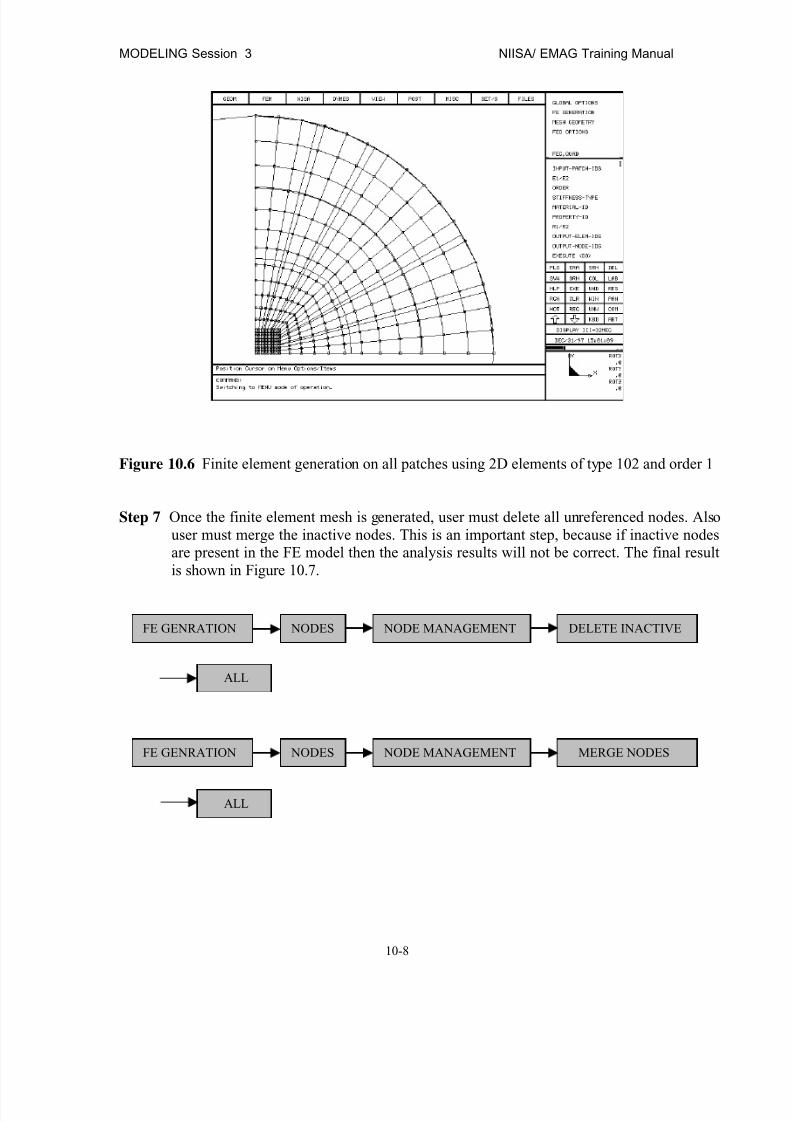
8/12/2019 emagtm
http://slidepdf.com/reader/full/emagtm 156/246
MODELING Session 3 NIISA/ EMAG Training Manual
10-8
Figure 10.6 Finite element generation on all patches using 2D elements of type 102 and order 1
Step 7 Once the finite element mesh is generated, user must delete all unreferenced nodes. Alsouser must merge the inactive nodes. This is an important step, because if inactive nodesare present in the FE model then the analysis results will not be correct. The final resultis shown in Figure 10.7.
FE GENRATION NODES NODE MANAGEMENT DELETE INACTIVE
ALL
FE GENRATION NODES NODE MANAGEMENT MERGE NODES
ALL

8/12/2019 emagtm
http://slidepdf.com/reader/full/emagtm 157/246
NISA/ EMAG Training Manual MODELING Session 3
10-9
Figure 10.7 Merging and deletion of inactive nodes
Step 8 Now user must define the material properties. In this capacitor problem there is only onematerial, that is, air. For air permittivity = 8.854 x 10⁻¹² F/m.
In order to define permittivity of air follow the command syntax (1), see forms shown in Figure10.8a and 10.8b respectively. User will define the material constants depending on the analysistypes. For the capacitor, the user should enter the permittivity of air in the first column of EXX .
(1)
OR
(1)
NISA DATA GROUP NISA FORMS MATERIALEFIELD
FE GENERATION FE MODEL DATA
ADD
MATERIAL DATA
ADD Emag
Emag
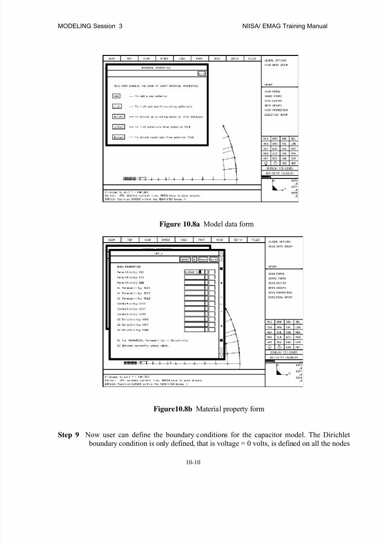
8/12/2019 emagtm
http://slidepdf.com/reader/full/emagtm 158/246
MODELING Session 3 NIISA/ EMAG Training Manual
10-10
Figure 10.8a Model data form
Figure10.8b Material property form
Step 9 Now user can define the boundary conditions for the capacitor model. The Dirichlet boundary condition is only defined, that is voltage = 0 volts, is defined on all the nodes

8/12/2019 emagtm
http://slidepdf.com/reader/full/emagtm 159/246
NISA/ EMAG Training Manual MODELING Session 3
10-11
corresponding to Figure 10.0b and voltage = 100 volts on the nodes lying on the upper plate, as shown in Figure 10.9.
Now, in SET-ID put set-id number 1 (say); in SPEC. FIELD POT put value 0.0 and in NODE-ID select BORDER and choose the nodes stated earlier. Use left mouse button for each of them.Repeat the same with SPEC. FIELD POT as 100 for nodes on the upper plate.
Figure 10.9 Dirichlet boundary condition
Step 10 Finally, user must define the title, the EMAG control, and the executive command cards
such as analysis type, and sub analysis type. The forms of which are shown in Figures10.10, 10.11 and 10.12 respectively. Follow the command sequences given below.
TITLE
FE GENERATION BOUNDARY CONDN. SPFPOTEMAG
NISA DATA GROUP NISA FORMS TITLEEFIELD
ADD ON NODES

8/12/2019 emagtm
http://slidepdf.com/reader/full/emagtm 160/246
MODELING Session 3 NIISA/ EMAG Training Manual
10-12
EMAG CONTROL
ANALYSIS / SUB ANALYSIS TYPE
Figure 10.10 Title form
NISA DATA GROUP NISA FORMS EMAG CONTROLEFIELD
NISA DATA GROUP NISA FORMS EXECUTIVE
SUBA
EFIELD
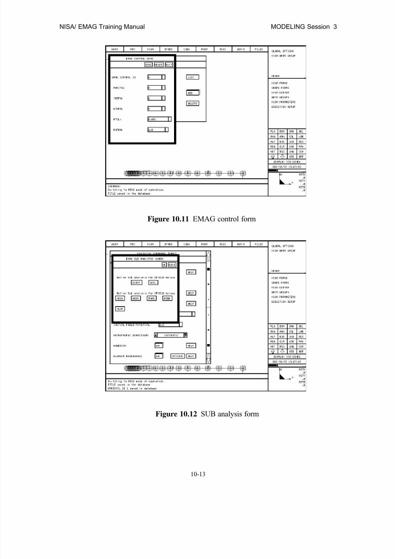
8/12/2019 emagtm
http://slidepdf.com/reader/full/emagtm 161/246
NISA/ EMAG Training Manual MODELING Session 3
10-13
Figure 10.11 EMAG control form
Figure 10.12 SUB analysis form

8/12/2019 emagtm
http://slidepdf.com/reader/full/emagtm 162/246
MODELING Session 3 NIISA/ EMAG Training Manual
10-14
Step 11 Futhermore, user must write .NIS, .DBS and .NEU files. NISA input file will be usedfor running the EMAG analysis, whereas .DBS (binary file) and NEU (ASCII file)contains the geometry and the finite element information of the model. The files arewritten by the following the procedure given below
Step 12 The program has its own editor and you may view and edit the NISA file. You areencouraged to view this file and understand the format of this file, which is thoroughlydocumented in the EMAG User’s manual. In many cases, you may make minorchanges and add more information regarding data groups which are not supportedthrough DISPLAY III. Figure 10.13 illustrates the NISA file.
FILE MANAGEMENT →→→→ EDIT →→→→ filename →→→→
The NISA input file will now appear on the screen. You may scroll the file by using thescrollbar at the right side of the screen. For now, do not attempt to make any changes inthe file. After viewing, exit the editor by clicking the mouse in the ‘QUIT’ box
FILE MANAGEMENT →→→→ WRITE →→→→ NISA FILE →→→→ filename →→→→
FILE MANAGEMENT →→→→ WRITE →→→→ DATABASE FILE →→→→ filename →→→→
FILE MANAGEMENT →→→→ WRITE →→→→ NEUTRAL FILE →→→→ filename →→→→
You should enter the name of the file in which you want to store the above files
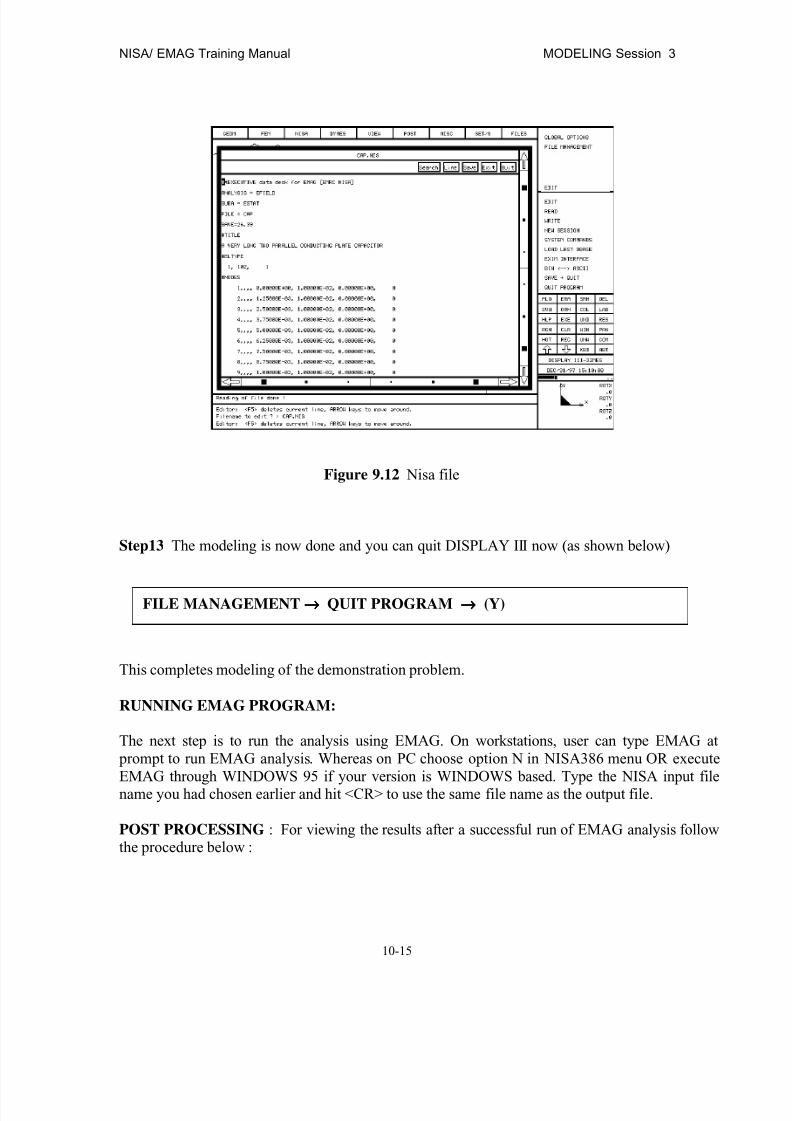
8/12/2019 emagtm
http://slidepdf.com/reader/full/emagtm 163/246
NISA/ EMAG Training Manual MODELING Session 3
10-15
Figure 9.12 Nisa file
Step13 The modeling is now done and you can quit DISPLAY III now (as shown below)
This completes modeling of the demonstration problem.
RUNNING EMAG PROGRAM:
The next step is to run the analysis using EMAG. On workstations, user can type EMAG at prompt to run EMAG analysis. Whereas on PC choose option N in NISA386 menu OR executeEMAG through WINDOWS 95 if your version is WINDOWS based. Type the NISA input filename you had chosen earlier and hit <CR> to use the same file name as the output file.
POST PROCESSING : For viewing the results after a successful run of EMAG analysis followthe procedure below :
FILE MANAGEMENT →→→→ QUIT PROGRAM →→→→ (Y)

8/12/2019 emagtm
http://slidepdf.com/reader/full/emagtm 164/246
MODELING Session 3 NIISA/ EMAG Training Manual
10-16
1)
2)
Now user will see the form which contain the output parameters to be post processed, see Figure10.14.
Figure 10.14 Form for picking the Voltage
In this example we have chosen the Voltage to be viewed. Figure 10.15 shows the contour linesof the Voltage distribution.
FILE MANAGEMENT READ POST FILES
POST RESULTS CONTOURS PICK RESULTS

8/12/2019 emagtm
http://slidepdf.com/reader/full/emagtm 165/246
NISA/ EMAG Training Manual MODELING Session 3
10-17
Figure 10.15 The Voltage distribution
You can see the resultant electric field arrow plots using the following command sequence. Thisis shown in Figure 10.16
POST RESULTS MISC. RESULTS EMAG ARROW PLOTS
ELECTRIC FIELD
VIEW DISPLAY OPTIONS BOUNDARY LINE
ALL ELEMENTS
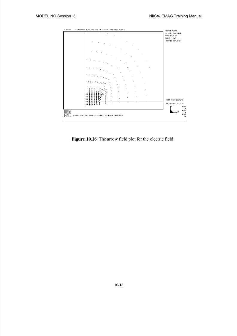
8/12/2019 emagtm
http://slidepdf.com/reader/full/emagtm 166/246
MODELING Session 3 NIISA/ EMAG Training Manual
10-18
Figure 10.16 The arrow field plot for the electric field
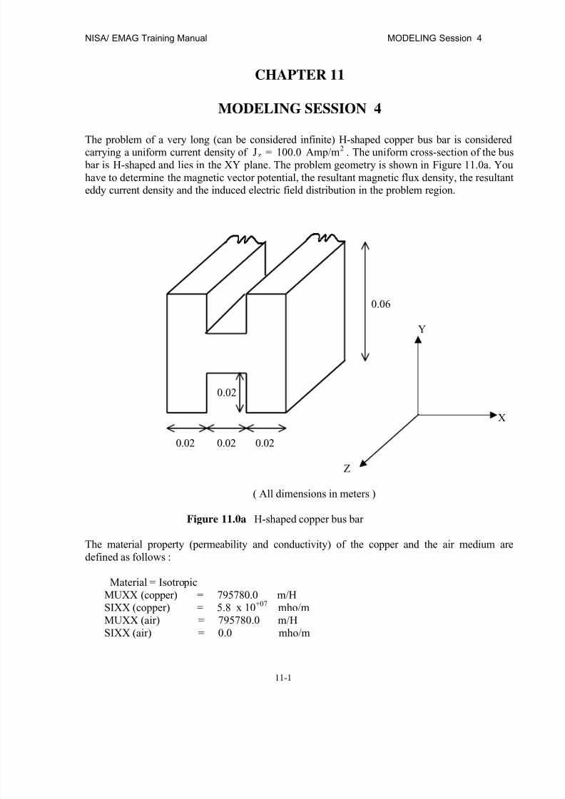
8/12/2019 emagtm
http://slidepdf.com/reader/full/emagtm 167/246
NISA/ EMAG Training Manual MODELING Session 4
11-1
CHAPTER 11
MODELING SESSION 4
The problem of a very long (can be considered infinite) H-shaped copper bus bar is consideredcarrying a uniform current density of Jz = 100.0 Amp/m2 . The uniform cross-section of the bus bar is H-shaped and lies in the XY plane. The problem geometry is shown in Figure 11.0a. Youhave to determine the magnetic vector potential, the resultant magnetic flux density, the resultanteddy current density and the induced electric field distribution in the problem region.
0.06
Y
0.02
X
0.02 0.02 0.02
Z
( All dimensions in meters )
Figure 11.0a H-shaped copper bus bar
The material property (permeability and conductivity) of the copper and the air medium are
defined as follows :
Material = IsotropicMUXX (copper) = 795780.0 m/HSIXX (copper) = 5.8 x 10+07 mho/mMUXX (air) = 795780.0 m/HSIXX (air) = 0.0 mho/m
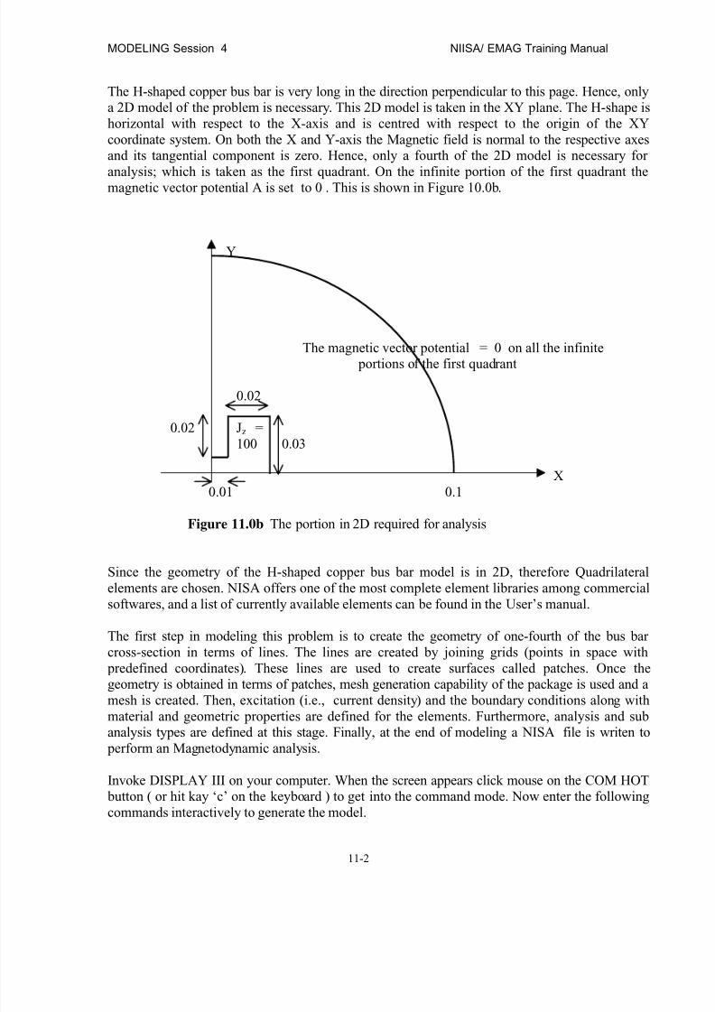
8/12/2019 emagtm
http://slidepdf.com/reader/full/emagtm 168/246
MODELING Session 4 NIISA/ EMAG Training Manual
11-2
The H-shaped copper bus bar is very long in the direction perpendicular to this page. Hence, onlya 2D model of the problem is necessary. This 2D model is taken in the XY plane. The H-shape ishorizontal with respect to the X-axis and is centred with respect to the origin of the XYcoordinate system. On both the X and Y-axis the Magnetic field is normal to the respective axesand its tangential component is zero. Hence, only a fourth of the 2D model is necessary for
analysis; which is taken as the first quadrant. On the infinite portion of the first quadrant themagnetic vector potential A is set to 0 . This is shown in Figure 10.0b.
Y
The magnetic vector potential = 0 on all the infinite portions of the first quadrant
0.02
0.02 Jz =100 0.03
X0.01 0.1
Figure 11.0b The portion in 2D required for analysis
Since the geometry of the H-shaped copper bus bar model is in 2D, therefore Quadrilateralelements are chosen. NISA offers one of the most complete element libraries among commercialsoftwares, and a list of currently available elements can be found in the User’s manual.
The first step in modeling this problem is to create the geometry of one-fourth of the bus barcross-section in terms of lines. The lines are created by joining grids (points in space with predefined coordinates). These lines are used to create surfaces called patches. Once thegeometry is obtained in terms of patches, mesh generation capability of the package is used and amesh is created. Then, excitation (i.e., current density) and the boundary conditions along withmaterial and geometric properties are defined for the elements. Furthermore, analysis and subanalysis types are defined at this stage. Finally, at the end of modeling a NISA file is writen to perform an Magnetodynamic analysis.
Invoke DISPLAY III on your computer. When the screen appears click mouse on the COM HOT button ( or hit kay ‘c’ on the keyboard ) to get into the command mode. Now enter the followingcommands interactively to generate the model.

8/12/2019 emagtm
http://slidepdf.com/reader/full/emagtm 169/246
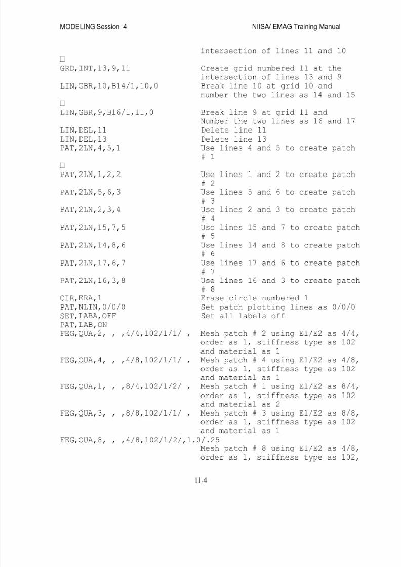
8/12/2019 emagtm
http://slidepdf.com/reader/full/emagtm 170/246
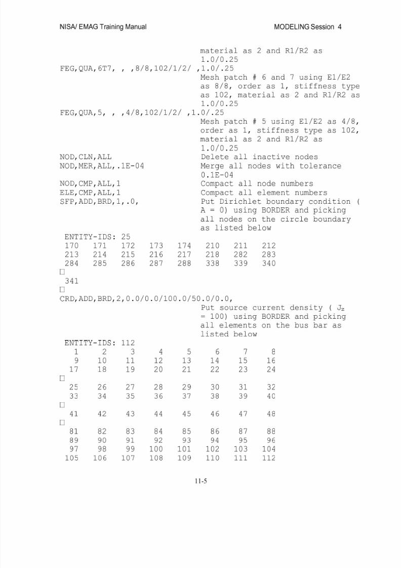
8/12/2019 emagtm
http://slidepdf.com/reader/full/emagtm 171/246
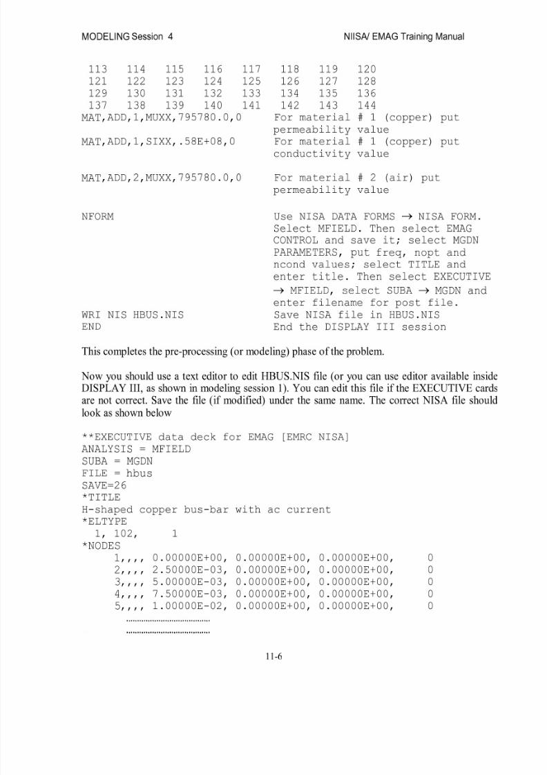
8/12/2019 emagtm
http://slidepdf.com/reader/full/emagtm 172/246

8/12/2019 emagtm
http://slidepdf.com/reader/full/emagtm 173/246
8/12/2019 emagtm
http://slidepdf.com/reader/full/emagtm 174/246

8/12/2019 emagtm
http://slidepdf.com/reader/full/emagtm 175/246
MODELING Session 4 NIISA/ EMAG Training Manual
11-48
Figure 11.1 Distribution of real part of the magnetic vector potential

8/12/2019 emagtm
http://slidepdf.com/reader/full/emagtm 176/246
NISA/ EMAG Training Manual MODELING Session 4
11-49
This page intentionally left blank
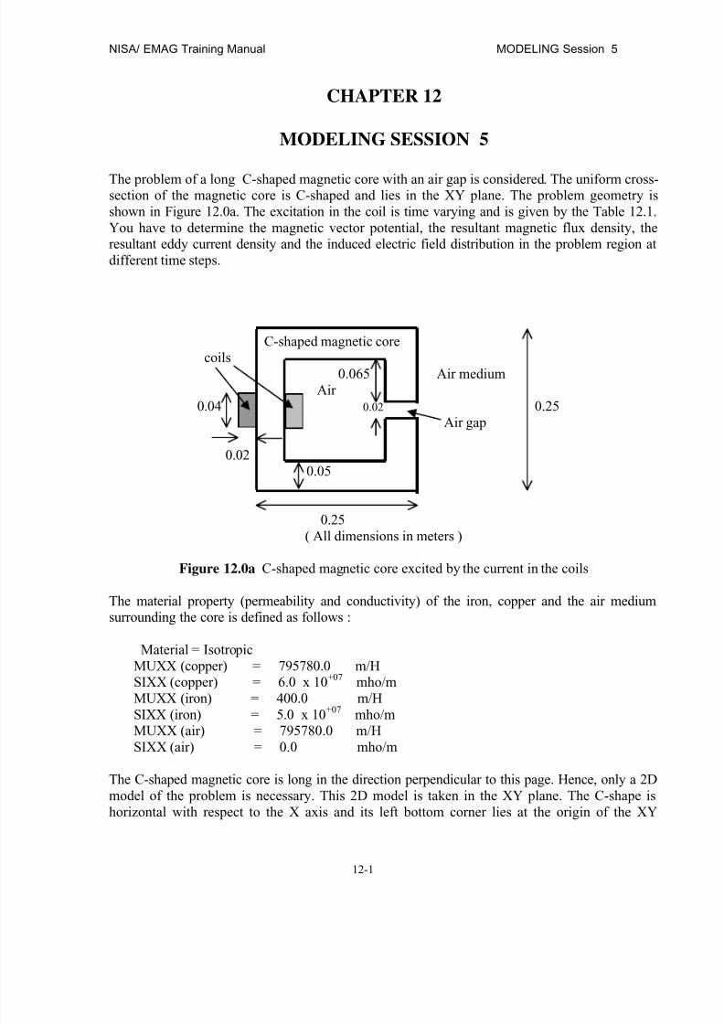
8/12/2019 emagtm
http://slidepdf.com/reader/full/emagtm 177/246
NISA/ EMAG Training Manual MODELING Session 5
12-1
CHAPTER 12
MODELING SESSION 5
The problem of a long C-shaped magnetic core with an air gap is considered. The uniform cross-section of the magnetic core is C-shaped and lies in the XY plane. The problem geometry isshown in Figure 12.0a. The excitation in the coil is time varying and is given by the Table 12.1.You have to determine the magnetic vector potential, the resultant magnetic flux density, theresultant eddy current density and the induced electric field distribution in the problem region atdifferent time steps.
C-shaped magnetic core
coils0.065 Air medium
Air0.04 0.02 0.25
Air gap
0.020.05
0.25
( All dimensions in meters )
Figure 12.0a C-shaped magnetic core excited by the current in the coils
The material property (permeability and conductivity) of the iron, copper and the air mediumsurrounding the core is defined as follows :
Material = IsotropicMUXX (copper) = 795780.0 m/HSIXX (copper) = 6.0 x 10+07 mho/mMUXX (iron) = 400.0 m/H
SIXX (iron) = 5.0 x 10+07
mho/mMUXX (air) = 795780.0 m/HSIXX (air) = 0.0 mho/m
The C-shaped magnetic core is long in the direction perpendicular to this page. Hence, only a 2Dmodel of the problem is necessary. This 2D model is taken in the XY plane. The C-shape ishorizontal with respect to the X axis and its left bottom corner lies at the origin of the XY
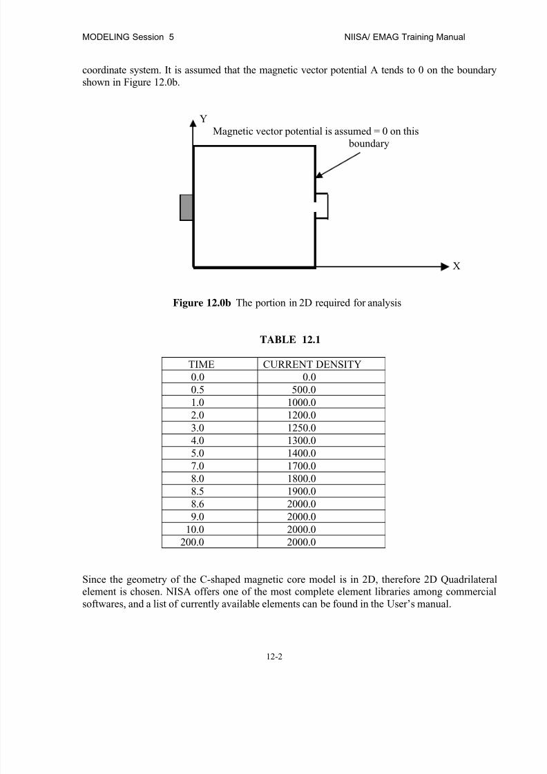
8/12/2019 emagtm
http://slidepdf.com/reader/full/emagtm 178/246
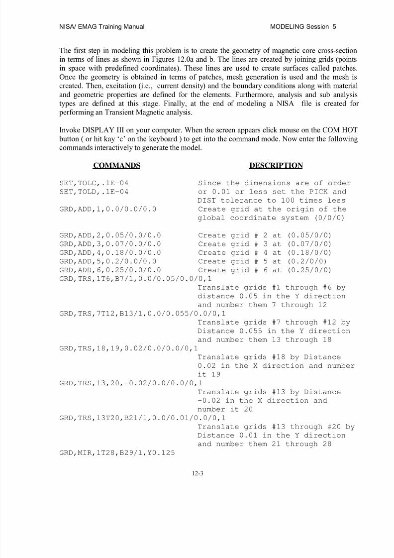
8/12/2019 emagtm
http://slidepdf.com/reader/full/emagtm 179/246
NISA/ EMAG Training Manual MODELING Session 5
12-3
The first step in modeling this problem is to create the geometry of magnetic core cross-sectionin terms of lines as shown in Figures 12.0a and b. The lines are created by joining grids (pointsin space with predefined coordinates). These lines are used to create surfaces called patches.Once the geometry is obtained in terms of patches, mesh generation is used and the mesh iscreated. Then, excitation (i.e., current density) and the boundary conditions along with material
and geometric properties are defined for the elements. Furthermore, analysis and sub analysistypes are defined at this stage. Finally, at the end of modeling a NISA file is created for performing an Transient Magnetic analysis.
Invoke DISPLAY III on your computer. When the screen appears click mouse on the COM HOT button ( or hit kay ‘c’ on the keyboard ) to get into the command mode. Now enter the followingcommands interactively to generate the model.
COMMANDS DESCRIPTION
SET,TOLC,.1E-04 Since the dimensions are of order
SET,TOLD,.1E-04 or 0.01 or less set the PICK and
DIST tolerance to 100 times less
GRD,ADD,1,0.0/0.0/0.0 Create grid at the origin of the
global coordinate system (0/0/0)
GRD,ADD,2,0.05/0.0/0.0 Create grid # 2 at (0.05/0/0)
GRD,ADD,3,0.07/0.0/0.0 Create grid # 3 at (0.07/0/0)
GRD,ADD,4,0.18/0.0/0.0 Create grid # 4 at (0.18/0/0)
GRD,ADD,5,0.2/0.0/0.0 Create grid # 5 at (0.2/0/0)
GRD,ADD,6,0.25/0.0/0.0 Create grid # 6 at (0.25/0/0)
GRD,TRS,1T6,B7/1,0.0/0.05/0.0/0,1
Translate grids #1 through #6 by
distance 0.05 in the Y direction
and number them 7 through 12
GRD,TRS,7T12,B13/1,0.0/0.055/0.0/0,1
Translate grids #7 through #12 by
Distance 0.055 in the Y direction
and number them 13 through 18
GRD,TRS,18,19,0.02/0.0/0.0/0,1
Translate grids #18 by Distance
0.02 in the X direction and number
it 19
GRD,TRS,13,20,-0.02/0.0/0.0/0,1
Translate grids #13 by Distance-0.02 in the X direction and
number it 20
GRD,TRS,13T20,B21/1,0.0/0.01/0.0/0,1
Translate grids #13 through #20 by
Distance 0.01 in the Y direction
and number them 21 through 28
GRD,MIR,1T28,B29/1,Y0.125

8/12/2019 emagtm
http://slidepdf.com/reader/full/emagtm 180/246
MODELING Session 5 NIISA/ EMAG Training Manual
12-4
Mirror grids #1 through #28 about
XZ plane at Y = 0.125 and number
them 29 through 56
LIN,2GD,1,2,1 Join grids 1, 2 to create line # 1
LIN,2GD,2,3,2 Join grids 2, 3 to create line # 2
LIN,2GD,3,4,3 Join grids 3, 4 to create line # 3
LIN,2GD,4,5,4 Join grids 4, 5 to create line # 4
LIN,2GD,5,6,5 Join grids 5, 6 to create line # 5
LIN,2GD,7,8,6 Join grids 7, 8 to create line # 6
LIN,2GD,8,9,7 Join grids 8, 9 to create line # 7
LIN,2GD,9,10,8 Join grids 9, 10 to create line #8
LIN,2GD,10,11,9 Join grids 10,11 to create line #9
LIN,2GD,11,12,10 Join grids 11,12 to create line #
10
LIN,2GD,20,13,11 Join grids 20,13 to create line #
11
LIN,2GD,13,14,12 Join grids 13,14 to create line #
12
LIN,2GD,14,15,13 Join grids 14,15 to create line #
13
LIN,2GD,15,16,14 Join grids 15,16 to create line #
14
LIN,2GD,16,17,15 Join grids 16,17 to create line #
15
LIN,2GD,17,18,16 Join grids 17,18 to create line #
16
LIN,2GD,18,19,17 Join grids 18,19 to create line #
17
LIN,2GD,28,21,18 Join grids 28,21 to create line #18
LIN,2GD,21,22,19 Join grids 21,22 to create line #
19
LIN,2GD,22,23,20 Join grids 22,23 to create line #
20
LIN,2GD,23,24,21 Join grids 23,24 to create line #
21
LIN,2GD,24,25,22 Join grids 24,25 to create line #
22
LIN,2GD,25,26,23 Join grids 25,26 to create line #
23LIN,2GD,26,27,24 Join grids 26,27 to create line #
24
LIN,MIR,1T24,B27/1,Y0.125 Mirror lines 1 through 24 about
the XZ plane at Y = 0.125 creating
lines starting at numbers 27
PAT,2LN,6,1,1 Use lines 6 and 1 to create patch
# 1
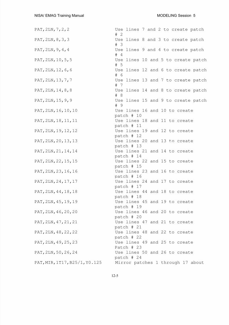
8/12/2019 emagtm
http://slidepdf.com/reader/full/emagtm 181/246
NISA/ EMAG Training Manual MODELING Session 5
12-5
PAT,2LN,7,2,2 Use lines 7 and 2 to create patch
# 2
PAT,2LN,8,3,3 Use lines 8 and 3 to create patch
# 3
PAT,2LN,9,4,4 Use lines 9 and 4 to create patch
# 4
PAT,2LN,10,5,5 Use lines 10 and 5 to create patch
# 5
PAT,2LN,12,6,6 Use lines 12 and 6 to create patch
# 6
PAT,2LN,13,7,7 Use lines 13 and 7 to create patch
# 7
PAT,2LN,14,8,8 Use lines 14 and 8 to create patch
# 8
PAT,2LN,15,9,9 Use lines 15 and 9 to create patch
# 9
PAT,2LN,16,10,10 Use lines 16 and 10 to create
patch # 10
PAT,2LN,18,11,11 Use lines 18 and 11 to create
patch # 11
PAT,2LN,19,12,12 Use lines 19 and 12 to create
patch # 12
PAT,2LN,20,13,13 Use lines 20 and 13 to create
patch # 13
PAT,2LN,21,14,14 Use lines 21 and 14 to create
patch # 14
PAT,2LN,22,15,15 Use lines 22 and 15 to create
patch # 15
PAT,2LN,23,16,16 Use lines 23 and 16 to createpatch # 16
PAT,2LN,24,17,17 Use lines 24 and 17 to create
patch # 17
PAT,2LN,44,18,18 Use lines 44 and 18 to create
patch # 18
PAT,2LN,45,19,19 Use lines 45 and 19 to create
patch # 19
PAT,2LN,46,20,20 Use lines 46 and 20 to create
patch # 20
PAT,2LN,47,21,21 Use lines 47 and 21 to create
patch # 21PAT,2LN,48,22,22 Use lines 48 and 22 to create
patch # 22
PAT,2LN,49,25,23 Use lines 49 and 25 to create
Patch # 23
PAT,2LN,50,26,24 Use lines 50 and 26 to create
patch # 24
PAT,MIR,1T17,B25/1,Y0.125 Mirror patches 1 through 17 about
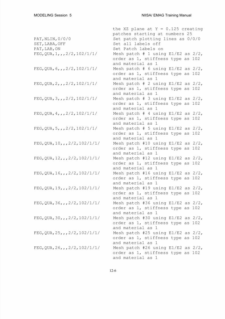
8/12/2019 emagtm
http://slidepdf.com/reader/full/emagtm 182/246
MODELING Session 5 NIISA/ EMAG Training Manual
12-6
the XZ plane at Y = 0.125 creating
patches starting at numbers 25
PAT,NLIN,0/0/0 Set patch plotting lines as 0/0/0
SET,LABA,OFF Set all labels off
PAT,LAB,ON Set Patch labels on
FEG,QUA,1,,,2/2,102/1/1/ Mesh patch # 1 using E1/E2 as 2/2,
order as 1, stiffness type as 102
and material as 1
FEG,QUA,6,,,2/2,102/1/1/ Mesh patch # 6 using E1/E2 as 2/2,
order as 1, stiffness type as 102
and material as 1
FEG,QUA,2,,,2/2,102/1/1/ Mesh patch # 2 using E1/E2 as 2/2,
order as 1, stiffness type as 102
and material as 1
FEG,QUA,3,,,2/2,102/1/1/ Mesh patch # 3 using E1/E2 as 2/2,
order as 1, stiffness type as 102
and material as 1
FEG,QUA,4,,,2/2,102/1/1/ Mesh patch # 4 using E1/E2 as 2/2,
order as 1, stiffness type as 102
and material as 1
FEG,QUA,5,,,2/2,102/1/1/ Mesh patch # 5 using E1/E2 as 2/2,
order as 1, stiffness type as 102
and material as 1
FEG,QUA,10,,,2/2,102/1/1/ Mesh patch #10 using E1/E2 as 2/2,
order as 1, stiffness type as 102
and material as 1
FEG,QUA,12,,,2/2,102/1/1/ Mesh patch #12 using E1/E2 as 2/2,
order as 1, stiffness type as 102
and material as 1FEG,QUA,16,,,2/2,102/1/1/ Mesh patch #16 using E1/E2 as 2/2,
order as 1, stiffness type as 102
and material as 1
FEG,QUA,19,,,2/2,102/1/1/ Mesh patch #19 using E1/E2 as 2/2,
order as 1, stiffness type as 102
and material as 1
FEG,QUA,36,,,2/2,102/1/1/ Mesh patch #36 using E1/E2 as 2/2,
order as 1, stiffness type as 102
and material as 1
FEG,QUA,30,,,2/2,102/1/1/ Mesh patch #30 using E1/E2 as 2/2,
order as 1, stiffness type as 102and material as 1
FEG,QUA,25,,,2/2,102/1/1/ Mesh patch #25 using E1/E2 as 2/2,
order as 1, stiffness type as 102
and material as 1
FEG,QUA,26,,,2/2,102/1/1/ Mesh patch #26 using E1/E2 as 2/2,
order as 1, stiffness type as 102
and material as 1

8/12/2019 emagtm
http://slidepdf.com/reader/full/emagtm 183/246
NISA/ EMAG Training Manual MODELING Session 5
12-7
FEG,QUA,27,,,2/2,102/1/1/ Mesh patch #27 using E1/E2 as 2/2,
order as 1, stiffness type as 102
and material as 1
FEG,QUA,28,,,2/2,102/1/1/ Mesh patch #28 using E1/E2 as 2/2,
order as 1, stiffness type as 102
and material as 1
FEG,QUA,29,,,2/2,102/1/1/ Mesh patch #29 using E1/E2 as 2/2,
order as 1, stiffness type as 102
and material as 1
FEG,QUA,34,,,2/2,102/1/1/ Mesh patch #34 using E1/E2 as 2/2,
order as 1, stiffness type as 102
and material as 1
FEG,QUA,40,,,2/2,102/1/1/ Mesh patch #40 using E1/E2 as 2/2,
order as 1, stiffness type as 102
and material as 1
FEG,QUA,23,,,2/2,102/1/2/ Mesh patch #23 using E1/E2 as 2/2,
order as 1, stiffness type as 102
and material as 2
FEG,QUA,22,,,2/2,102/1/2/ Mesh patch #22 using E1/E2 as 2/2,
order as 1, stiffness type as 102
and material as 2
FEG,QUA,24,,,2/2,102/1/2/ Mesh patch #24 using E1/E2 as 2/2,
order as 1, stiffness type as 102
and material as 2
FEG,QUA,7,,,2/2,102/1/2/ Mesh patch # 7 using E1/E2 as 2/2,
order as 1, stiffness type as 102
and material as 2
FEG,QUA,8,,,2/2,102/1/2/ Mesh patch # 8 using E1/E2 as 2/2,
order as 1, stiffness type as 102and material as 2
FEG,QUA,9,,,2/2,102/1/2/ Mesh patch # 9 using E1/E2 as 2/2,
order as 1, stiffness type as 102
and material as 2
FEG,QUA,14,,,2/2,102/1/2/ Mesh patch #14 using E1/E2 as 2/2,
order as 1, stiffness type as 102
and material as 2
FEG,QUA,21,,,2/2,102/1/2/ Mesh patch #21 using E1/E2 as 2/2,
order as 1, stiffness type as 102
and material as 2
FEG,QUA,31,,,2/2,102/1/2/ Mesh patch #31 using E1/E2 as 2/2,order as 1, stiffness type as 102
and material as 2
FEG,QUA,32,,,2/2,102/1/2/ Mesh patch #32 using E1/E2 as 2/2,
order as 1, stiffness type as 102
and material as 2
FEG,QUA,33,,,2/2,102/1/2/ Mesh patch #33 using E1/E2 as 2/2,
order as 1, stiffness type as 102
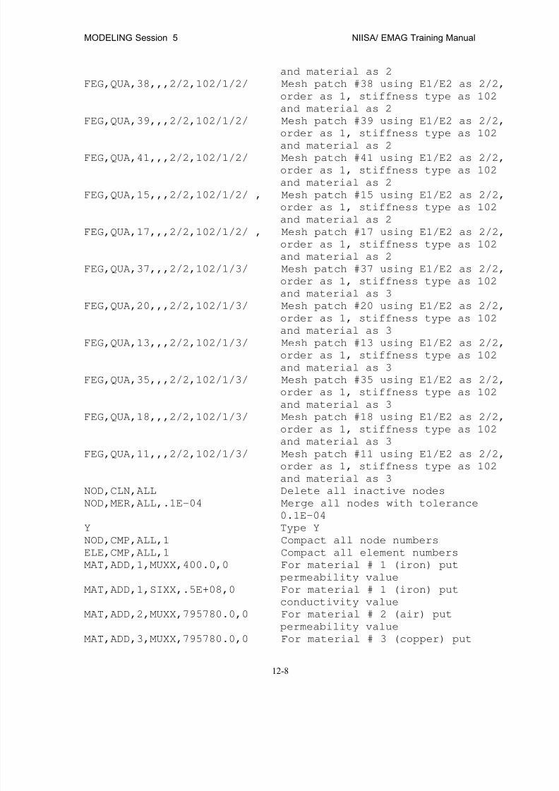
8/12/2019 emagtm
http://slidepdf.com/reader/full/emagtm 184/246
MODELING Session 5 NIISA/ EMAG Training Manual
12-8
and material as 2
FEG,QUA,38,,,2/2,102/1/2/ Mesh patch #38 using E1/E2 as 2/2,
order as 1, stiffness type as 102
and material as 2
FEG,QUA,39,,,2/2,102/1/2/ Mesh patch #39 using E1/E2 as 2/2,
order as 1, stiffness type as 102
and material as 2
FEG,QUA,41,,,2/2,102/1/2/ Mesh patch #41 using E1/E2 as 2/2,
order as 1, stiffness type as 102
and material as 2
FEG,QUA,15,,,2/2,102/1/2/ , Mesh patch #15 using E1/E2 as 2/2,
order as 1, stiffness type as 102
and material as 2
FEG,QUA,17,,,2/2,102/1/2/ , Mesh patch #17 using E1/E2 as 2/2,
order as 1, stiffness type as 102
and material as 2
FEG,QUA,37,,,2/2,102/1/3/ Mesh patch #37 using E1/E2 as 2/2,
order as 1, stiffness type as 102
and material as 3
FEG,QUA,20,,,2/2,102/1/3/ Mesh patch #20 using E1/E2 as 2/2,
order as 1, stiffness type as 102
and material as 3
FEG,QUA,13,,,2/2,102/1/3/ Mesh patch #13 using E1/E2 as 2/2,
order as 1, stiffness type as 102
and material as 3
FEG,QUA,35,,,2/2,102/1/3/ Mesh patch #35 using E1/E2 as 2/2,
order as 1, stiffness type as 102
and material as 3
FEG,QUA,18,,,2/2,102/1/3/ Mesh patch #18 using E1/E2 as 2/2,order as 1, stiffness type as 102
and material as 3
FEG,QUA,11,,,2/2,102/1/3/ Mesh patch #11 using E1/E2 as 2/2,
order as 1, stiffness type as 102
and material as 3
NOD,CLN,ALL Delete all inactive nodes
NOD,MER,ALL,.1E-04 Merge all nodes with tolerance
0.1E-04
Y Type Y
NOD,CMP,ALL,1 Compact all node numbers
ELE,CMP,ALL,1 Compact all element numbersMAT,ADD,1,MUXX,400.0,0 For material # 1 (iron) put
permeability value
MAT,ADD,1,SIXX,.5E+08,0 For material # 1 (iron) put
conductivity value
MAT,ADD,2,MUXX,795780.0,0 For material # 2 (air) put
permeability value
MAT,ADD,3,MUXX,795780.0,0 For material # 3 (copper) put
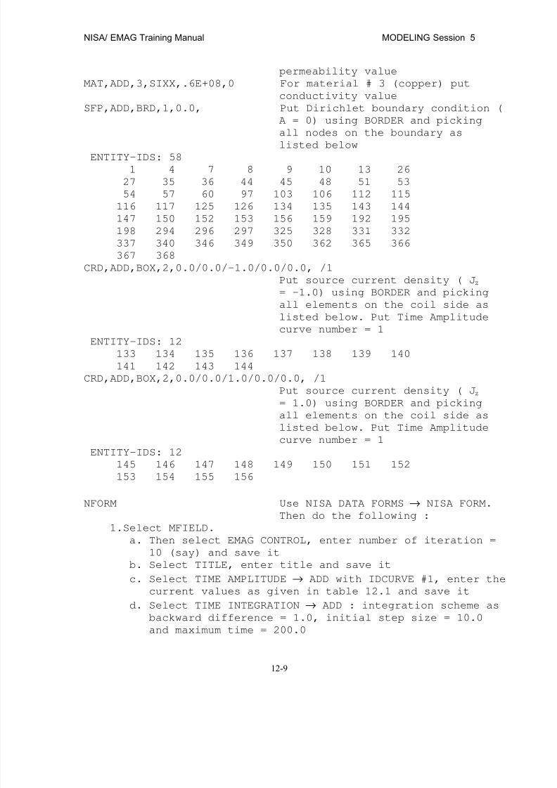
8/12/2019 emagtm
http://slidepdf.com/reader/full/emagtm 185/246
NISA/ EMAG Training Manual MODELING Session 5
12-9
permeability value
MAT,ADD,3,SIXX,.6E+08,0 For material # 3 (copper) put
conductivity value
SFP,ADD,BRD,1,0.0, Put Dirichlet boundary condition (
A = 0) using BORDER and picking
all nodes on the boundary as
listed below
ENTITY-IDS: 58
1 4 7 8 9 10 13 26
27 35 36 44 45 48 51 53
54 57 60 97 103 106 112 115
116 117 125 126 134 135 143 144
147 150 152 153 156 159 192 195
198 294 296 297 325 328 331 332
337 340 346 349 350 362 365 366
367 368
CRD,ADD,BOX,2,0.0/0.0/-1.0/0.0/0.0, /1
Put source current density ( Jz
= -1.0) using BORDER and picking
all elements on the coil side as
listed below. Put Time Amplitude
curve number = 1
ENTITY-IDS: 12
133 134 135 136 137 138 139 140
141 142 143 144
CRD,ADD,BOX,2,0.0/0.0/1.0/0.0/0.0, /1
Put source current density ( Jz
= 1.0) using BORDER and picking
all elements on the coil side aslisted below. Put Time Amplitude
curve number = 1
ENTITY-IDS: 12
145 146 147 148 149 150 151 152
153 154 155 156
NFORM Use NISA DATA FORMS → NISA FORM.
Then do the following :
1.Select MFIELD.
a. Then select EMAG CONTROL, enter number of iteration =
10 (say) and save itb. Select TITLE, enter title and save it
c. Select TIME AMPLITUDE → ADD with IDCURVE #1, enter the
current values as given in table 12.1 and save it
d. Select TIME INTEGRATION → ADD : integration scheme as
backward difference = 1.0, initial step size = 10.0
and maximum time = 200.0
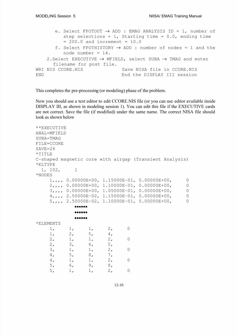
8/12/2019 emagtm
http://slidepdf.com/reader/full/emagtm 186/246
MODELING Session 5 NIISA/ EMAG Training Manual
12-10
e. Select FPOTOUT → ADD : EMAG ANALYSIS ID = 1, number of
step selections = 1, Starting time = 0.0, ending time
= 200.0 and increment = 10.0
f. Select FPOTHISTORY → ADD : number of nodes = 1 and the
node number = 14.
2.Select EXECUTIVE → MFIELD, select SUBA → TMAG and enterfilename for post file.
WRI NIS CCORE.NIS Save NISA file in CCORE.NIS
END End the DISPLAY III session
This completes the pre-processing (or modeling) phase of the problem.
Now you should use a text editor to edit CCORE.NIS file (or you can use editor available insideDISPLAY III, as shown in modeling session 1). You can edit this file if the EXECUTIVE cardsare not correct. Save the file (if modified) under the same name. The correct NISA file should
look as shown below
**EXECUTIVE
ANAL=MFIELD
SUBA=TMAG
FILE=CCORE
SAVE=26
*TITLE
C-shaped magnetic core with airgap (Transient Analysis)
*ELTYPE
1, 102, 1
*NODES1,,,, 0.00000E+00, 1.15000E-01, 0.00000E+00, 0
2,,,, 0.00000E+00, 1.10000E-01, 0.00000E+00, 0
3,,,, 0.00000E+00, 1.05000E-01, 0.00000E+00, 0
4,,,, 2.50000E-02, 1.15000E-01, 0.00000E+00, 0
5,,,, 2.50000E-02, 1.10000E-01, 0.00000E+00, 0
••••••
••••••
••••••
*ELEMENTS
1, 1, 1, 2, 0
1, 2, 5, 4,2, 1, 1, 2, 0
2, 3, 6, 5,
3, 1, 1, 2, 0
4, 5, 8, 7,
4, 1, 1, 2, 0
5, 6, 9, 8,
5, 1, 1, 2, 0
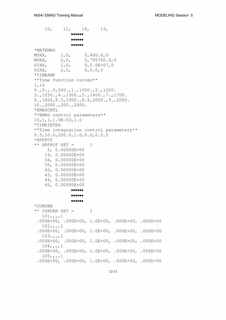
8/12/2019 emagtm
http://slidepdf.com/reader/full/emagtm 187/246
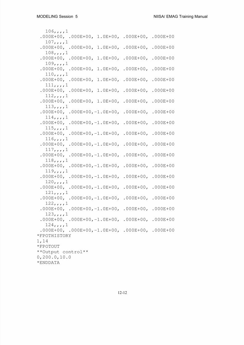
8/12/2019 emagtm
http://slidepdf.com/reader/full/emagtm 188/246
MODELING Session 5 NIISA/ EMAG Training Manual
12-12
106,,,,1
.000E+00, .000E+00, 1.0E+00, .000E+00, .000E+00
107,,,,1
.000E+00, .000E+00, 1.0E+00, .000E+00, .000E+00
108,,,,1
.000E+00, .000E+00, 1.0E+00, .000E+00, .000E+00
109,,,,1
.000E+00, .000E+00, 1.0E+00, .000E+00, .000E+00
110,,,,1
.000E+00, .000E+00, 1.0E+00, .000E+00, .000E+00
111,,,,1
.000E+00, .000E+00, 1.0E+00, .000E+00, .000E+00
112,,,,1
.000E+00, .000E+00, 1.0E+00, .000E+00, .000E+00
113,,,,1
.000E+00, .000E+00,-1.0E+00, .000E+00, .000E+00
114,,,,1
.000E+00, .000E+00,-1.0E+00, .000E+00, .000E+00
115,,,,1
.000E+00, .000E+00,-1.0E+00, .000E+00, .000E+00
116,,,,1
.000E+00, .000E+00,-1.0E+00, .000E+00, .000E+00
117,,,,1
.000E+00, .000E+00,-1.0E+00, .000E+00, .000E+00
118,,,,1
.000E+00, .000E+00,-1.0E+00, .000E+00, .000E+00
119,,,,1
.000E+00, .000E+00,-1.0E+00, .000E+00, .000E+00
120,,,,1.000E+00, .000E+00,-1.0E+00, .000E+00, .000E+00
121,,,,1
.000E+00, .000E+00,-1.0E+00, .000E+00, .000E+00
122,,,,1
.000E+00, .000E+00,-1.0E+00, .000E+00, .000E+00
123,,,,1
.000E+00, .000E+00,-1.0E+00, .000E+00, .000E+00
124,,,,1
.000E+00, .000E+00,-1.0E+00, .000E+00, .000E+00
*FPOTHISTORY
1,14*FPOTOUT
**Output control**
0,200.0,10.0
*ENDDATA

8/12/2019 emagtm
http://slidepdf.com/reader/full/emagtm 189/246
NISA/ EMAG Training Manual MODELING Session 5
12-13
Now you can run the EMAG solver. For DOS version execute NISA386 and choose ELECTRO-MAG (N); for WINDOWS version run EMAGS; for WORKSTATIONS execute EMAG. AT prompt for the input file name type : CCORE.NIS and accept the default CCORE.OUT as theoutput file name.
POST-PROCESSING :
DISPLAY III can now be used to view the results of the analysis graphically. A file namedCCORE26.DAT will be created by the EMAG solver when you run it (remember you had giventhe post filename as CCORE). This file is needed for post-processing.
Invoke DISPLAY III on your computer. The EMRC logo appears on the screen and the programis ready for interactive usage. By default, the menu mode becomes active so that the user can usethe mouse to execute different commands interactively.
To use this manual effectively, we suggest that you get into the command mode and execute the
commands discussed here by typing in from keyboard. After getting comfortable with this procedure, you should experiment with the menu mode and follow similar steps for post- processing results.
To get into the command mode, you need to move the cursor into the area on the screendisplaying ‘COMMAND’ and hit the ENTER key. You may also type in the letter ‘C’ to get intothe command mode.
For this session only one plot is viewed. You are encouraged to make use of the on-line HELPoption and experiment with various other options available to generate other plots of interest.
For post-processing, type the following commands
COMMANDS DESCRIPTION
REA,POS,CCORE Read the post-processing data file
CTR,ADD,MVP Select contour as the
magnetic vector potential
CTR,CLB,LNUM Select contours with lines and
numbers
PST,CSS,1 Select plot for time = 0.0
PLO Plot the contours
PST,CSS,4 Select plot for time = 40.0
PLO Plot the contours

8/12/2019 emagtm
http://slidepdf.com/reader/full/emagtm 190/246

8/12/2019 emagtm
http://slidepdf.com/reader/full/emagtm 191/246
NISA/ EMAG Training Manual MODELING Session 5
12-15
Figure 12.2 The magnetic vector potential distribution at time t = 40.0 sec

8/12/2019 emagtm
http://slidepdf.com/reader/full/emagtm 192/246
MODELING Session 5 NIISA/ EMAG Training Manual
12-16
This page intentionally left blank

8/12/2019 emagtm
http://slidepdf.com/reader/full/emagtm 193/246
NISA/ EMAG Training Manual MODELING Session 6
13-1
CHAPTER 13
MODELING SESSION 6
The problem of a three dimensional transformer is considered. The transformer core is alignedwith the XY plane and is made of a magnetic material like steel. The coil is made of copper. The problem geometry is shown in Figure 13.0. The excitation in the coil is assumed to be DC. Youhave to determine the magnetic scalar potential, the resultant magnetic flux density and theresultant magnetic field intensity distribution in the problem region.
(All dimensions in metres)
Figure 13.0 3 Dimensional Transformer excited by a DC current in the one coil
Transformer :
l = 20 cmh = 20 cms = 16 cmw = 2 cmExterior Region :L = 20 cmH = 20 cmW = 11.5 cmCoil :lc = 4 cmwc = 0.5 cmJ = Jx = Jx =
1.6 x 10⁶ A/m2
Y
Z X
0=∂
∂
n
φ φ = 0
φ = 0
8/12/2019 emagtm
http://slidepdf.com/reader/full/emagtm 194/246
MODELING Session 6 NIISA/ EMAG Training Manual
13-2
The material property (permeability) of the steel, copper and the air medium surrounding thecore is defined as follows:
Material = IsotropicMUXX (steel) = 5.867 x 10-03 H/m
MUXX (air) = 12.56 x 10
-07
H/mMUXX (copper) = 12.56 x 10-07 H/m
The three-dimensional core of the Transformer is aligned with the XY plane. It can be easilyseen that the transformer is symmetric with respect to all the three coordinate planes viz : XY,YZ and ZX. Hence, only a one-eighth of the model of the problem is necessary for solution. It isassumed that the magnetic scalar potential φm tends to 0 on the boundary shown in Figure 13.0.
Since the geometry of the Transformer model is in 3D, 3D Hexahedral element is chosen. NISAoffers one of the most complete element libraries among commercial softwares, and a list ofcurrently available elements can be found in the User’s manual.
The first step in modeling this problem is to create the geometry of the transformer in terms oflines as shown in Figures 13.0. The lines are created by joining grids (points in space with predefined coordinates). These lines are used to create surfaces called patches. These plane patches are employed to create hyperpatches such that these hyperpatches fully cover thetransformer model. Once the geometry is obtained in terms of hyperpatches, mesh generation isused and the mesh is created. Then, excitation (i.e., DC current density) and the boundaryconditions along with material and geometric properties are defined for the elements.Furthermore, analysis and sub analysis types are defined at this stage. Finally, at the end ofmodeling a NISA file is obtained to perform a Three-dimensional Magnetostatic analysis usingthe magnetic scalar potential.
Invoke DISPLAY III on your computer. When the screen appears click mouse on the COM HOT button ( or hit kay ‘c’ on the keyboard ) to get into the command mode. Now enter the followingcommands interactively to generate the model.
COMMANDS DESCRIPTION
SET,TOLC,.1E-04 Since the dimensions are of order
SET,TOLD,.1E-04 or 0.01 or less set the PICK and
DIST tolerance to 100 times less
GRD,ADD,1,0/0/0 Create grid at the origin of the
global coordinate system (0/0/0)
GRD,ADD,2,0.02/0/0 Create grid # 2 at (0.02/0/0)
GRD,ADD,3,0.025/0/0 Create grid # 3 at (0.025/0/0)
GRD,ADD,4,0.08/0/0 Create grid # 4 at (0.08/0/0)
GRD,ADD,5,0.1/0/0 Create grid # 5 at (0.1/0/0)
GRD,TRS,1T5,B6/1,0.0/0.02/0.0/0,1
Translate grids 1 through 5 by
0.02 in Y direction
GRD,TRS,1T5,B11/1,0.0/0.08/0.0/0,1

8/12/2019 emagtm
http://slidepdf.com/reader/full/emagtm 195/246
NISA/ EMAG Training Manual MODELING Session 6
13-3
Translate grids 1 through 5 by
0.08 in Y direction
GRD,TRS,1T5,B16/1,0.0/0.1/0.0/0,1
Translate grids 1 through 5 by
0.1 in Y direction
GRD,TRS,1T5,B21/1,0.0/0.2/0.0/0,1
Translate grids 1 through 5 by
0.2 in Y direction
GRD,TRS,1/6/11/16/21,B26/1,0.2/0.0/0.0/0,1
Translate grids 1/6/11/16/21 by
0.2 in X direction
LIN,2GD,1,2,1 Join grids 1, 2 to create line # 1
LIN,2GD,2,3,2 Join grids 2, 3 to create line # 2
LIN,2GD,3,4,3 Join grids 3, 4 to create line # 3
LIN,2GD,4,5,4 Join grids 4, 5 to create line # 4
LIN,2GD,5,26,5 Join grids 5,26 to create line # 5
LIN,TRS,1T5,B6/1,.0/.02/.0/0,1
Translate lines 1 through 5 by
0.02 in the Y direction
LIN,TRS,1T5,B11/1,.0/.08/.0/0,1
Translate lines 1 through 5 by
0.08 in the Y direction
LIN,TRS,1T5,B16/1,.0/.1/.0/0,1
Translate lines 1 through 5 by
0.1 in the Y direction
LIN,TRS,1T5,B21/1,.0/.2/.0/0,1
Translate lines 1 through 5 by
0.2 in the Y direction
SET,LABA,OFF Set all labels offPAT,2LN,6,1,1 Use lines 6 and 1 to create patch
# 1
PAT,2LN,7,2,2 Use lines 7 and 2 to create patch
# 2
PAT,2LN,8,3,3 Use lines 8 and 3 to create patch
# 3
PAT,2LN,9,4,4 Use lines 9 and 4 to create patch
# 4
PAT,2LN,10,5,5 Use lines 10 and 5 to create patch
# 5
PAT,2LN,11,6,6 Use lines 11 and 6 to create patch# 6
PAT,2LN,12,7,7 Use lines 12 and 7 to create patch
# 7
PAT,2LN,13,8,8 Use lines 13 and 8 to create patch
# 8
PAT,2LN,14,9,9 Use lines 14 and 9 to create patch
# 9
8/12/2019 emagtm
http://slidepdf.com/reader/full/emagtm 196/246
MODELING Session 6 NIISA/ EMAG Training Manual
13-4
PAT,2LN,15,10,10 Use lines 15 & 10 to create patch
# 10
PAT,2LN,16,11,11 Use lines 16 & 11 to create patch
# 11
PAT,2LN,17,12,12 Use lines 17 & 12 to create patch
# 12
PAT,2LN,18,13,13 Use lines 18 & 13 to create patch
# 13
PAT,2LN,19,14,14 Use lines 19 & 14 to create patch
# 14
PAT,2LN,20,15,15 Use lines 20 & 15 to create patch
# 15
PAT,2LN,21,16,16 Use lines 21 & 16 to create patch
# 16
PAT,2LN,22,17,17 Use lines 22 & 17 to create patch
# 17
PAT,2LN,23,18,18 Use lines 23 & 18 to create patch
# 18
PAT,2LN,24,19,19 Use lines 24 & 19 to create patch
# 19
PAT,2LN,25,20,20 Use lines 25 & 20 to create patch
# 20
PAT,NLIN,0/0/0 Set patch plotting lines as 0/0/0
PAT,TRS,1T20,B21/1,0.0/0.0/-0.01/0,1
Translate patches #1 through # 20
by –0.01 in the Z direction
PAT,TRS,1T20,B41/1,0.0/0.0/-0.015/0,1
Translate patches #1 through # 20
by –0.015 in the Z directionPAT,TRS,1T20,B61/1,0.0/0.0/-0.115/0,1
Translate patches #1 through # 20
by –0.115 in the Z direction
HYP,2PA,1T20,21T40 Create hyperpatches by using patch
set from 1 to 20 and patch set
from 21 to 40
HYP,2PA,21T40,41T60 Create hyperpatches by using patch
set from 21 to 40 and patch set
from 41 to 60
HYP,2PA,41T60,61T80 Create hyperpatches by using patch
set from 41 to 60 and patch setfrom 61 to 80
HYP,NLIN,0/0/0 Set hyperpatch plotting lines as
0/0/0
VEW,HID,ON Put hidden lines for element
plotting on
ELE,PAI,MAT Set element painting by material
on
8/12/2019 emagtm
http://slidepdf.com/reader/full/emagtm 197/246

8/12/2019 emagtm
http://slidepdf.com/reader/full/emagtm 198/246
MODELING Session 6 NIISA/ EMAG Training Manual
13-6
FEG,HEX,17,,,1/6/2,//2/,1.0/0.25/1.0
Mesh hyperpatch #17 using E1/E2/E3
as 1/6/2,order as 1,stiffness type
as 104, R1/R2/R3 as 1.0/0.25/1.0
and material as 2
FEG,HEX,20,,,6/6/2,//2/,4.0/0.25/1.0
Mesh hyperpatch #20 using E1/E2/E3
as 6/6/2,order as 1,stiffness type
as 104, R1/R2/R3 as 1.0/0.25/1.0
and material as 2
FEG,HEX,21,,,3/3/1,104//3/,1.0/1.0/1.0
Mesh hyperpatch #21 using E1/E2/E3
as 3/3/1,order as 1,stiffness type
as 104, R1/R2/R3 as 1.0/1.0/1.0
and material as 3
FEG,HEX,22,,,1/3/1,104//3/,1.0/1.0/1.0
Mesh hyperpatch #22 using E1/E2/E3
as 1/3/1,order as 1,stiffness type
as 104, R1/R2/R3 as 1.0/1.0/1.0
and material as 3
FEG,HEX,24/31/34,,,3/3/1,104//2/,1.0/1.0/1.0
Mesh hyperpatches #24/31/34
using E1/E2/E3 as 3/3/1,order as
1,stiffness type as 104, R1/R2/R3
as 1.0/1.0/1.0 and material as 2
FEG,HEX,26/29,,,3/6/1,104//2/,1.0/1.0/1.0
Mesh hyperpatches #26/29 using
E1/E2/E3 as 3/6/1,order as
1,stiffness type as 104, R1/R2/R3as 1.0/1.0/1.0 and material as 2
FEG,HEX,23,,,6/3/1,104//2/,1.0/1.0/1.0
Mesh hyperpatch #23 using E1/E2/E3
as 6/3/1,order as 1,stiffness type
as 104, R1/R2/R3 as 1.0/1.0/1.0
and material as 2
FEG,HEX,27,,,1/6/1,104//2/,1.0/1.0/1.0
Mesh hyperpatch #27 using E1/E2/E3
as 1/6/1,order as 1,stiffness type
as 104, R1/R2/R3 as 1.0/1.0/1.0
and material as 2FEG,HEX,28,,,6/6/1,104//2/,1.0/1.0/1.0
Mesh hyperpatch #28 using E1/E2/E3
as 6/6/1,order as 1,stiffness type
as 104, R1/R2/R3 as 1.0/1.0/1.0
and material as 2
FEG,HEX,25/35,,,6/3/1,104//2/,4.0/1.0/1.0
Mesh hyperpatches #25/35 using

8/12/2019 emagtm
http://slidepdf.com/reader/full/emagtm 199/246
NISA/ EMAG Training Manual MODELING Session 6
13-7
E1/E2/E3 as 6/3/1,order as
1,stiffness type as 104, R1/R2/R3
as 4.0/1.0/1.0 and material as 2
FEG,HEX,30,,,6/6/1,104//2/,4.0/1.0/1.0
Mesh hyperpatch #30 using E1/E2/E3
as 6/6/1,order as 1,stiffness type
as 104, R1/R2/R3 as 4.0/1.0/1.0
and material as 2
FEG,HEX,36,,,3/6/1,104//2/,1.0/0.25/1.0
Mesh hyperpatch #36 using E1/E2/E3
as 3/6/1,order as 1,stiffness type
as 104, R1/R2/R3 as 1.0/0.25/1.0
and material as 2
FEG,HEX,37,,,1/6/1,104//2/,1.0/0.25/1.0
Mesh hyperpatch #37 using E1/E2/E3
as 1/6/1,order as 1,stiffness type
as 104, R1/R2/R3 as 1.0/0.25/1.0
and material as 2
FEG,HEX,38,,,6/6/1,104//2/,1.0/0.25/1.0
Mesh hyperpatch #38 using E1/E2/E3
as 6/6/1,order as 1,stiffness type
as 104, R1/R2/R3 as 1.0/0.25/1.0
and material as 2
FEG,HEX,39,,,3/6/1,104//2/,1.0/0.25/1.0
Mesh hyperpatch #39 using E1/E2/E3
as 3/6/1,order as 1,stiffness type
as 104, R1/R2/R3 as 1.0/0.25/1.0
and material as 2
FEG,HEX,40,,,6/6/1,104//2/,4.0/0.25/1.0Mesh hyperpatch #40 using E1/E2/E3
as 6/6/1,order as 1,stiffness type
as 104, R1/R2/R3 as 4.0/0.25/1.0
and material as 2
FEG,HEX,41/44/51/54,,,3/3/6,104//2/,1.0/1.0/4.0
Mesh hyperpatches #41/44/51/54
using E1/E2/E3 as 3/3/6,order as
1,stiffness type as 104, R1/R2/R3
as 1.0/1.0/4.0 and material as 2
FEG,HEX,46/49,,,3/6/6,104//2/,1.0/1.0/4.0
Mesh hyperpatch #46/49 usingE1/E2/E3 as 3/6/6,order as
1,stiffness type as 104, R1/R2/R3
as 1.0/1.0/4.0 and material as 2
FEG,HEX,43/53,,,6/3/6,104//2/,1.0/1.0/4.0
Mesh hyperpatches #43/53 using
E1/E2/E3 as 6/3/6,order as
1,stiffness type as 104, R1/R2/R3
8/12/2019 emagtm
http://slidepdf.com/reader/full/emagtm 200/246
MODELING Session 6 NIISA/ EMAG Training Manual
13-8
as 1.0/1.0/4.0 and material as 2
FEG,HEX,42/52,,,1/3/6,104//2/,1.0/1.0/4.0
Mesh hyperpatches #42/52 using
E1/E2/E3 as 1/3/6,order as
1,stiffness type as 104, R1/R2/R3
as 1.0/1.0/4.0 and material as 2
FEG,HEX,47,,,1/6/6,104//2/,1.0/1.0/4.0
Mesh hyperpatch #47 using E1/E2/E3
as 1/6/6,order as 1,stiffness type
as 104, R1/R2/R3 as 1.0/1.0/4.0
and material as 2
FEG,HEX,48,,,6/6/6,104//2/,1.0/1.0/4.0
Mesh hyperpatch #48 using E1/E2/E3
as 6/6/6,order as 1,stiffness type
as 104, R1/R2/R3 as 1.0/1.0/4.0
and material as 2
FEG,HEX,45/55,,,6/3/6,104//2/,4.0/1.0/4.0
Mesh hyperpatches #45/55 using
E1/E2/E3 as 6/3/6,order as
1,stiffness type as 104, R1/R2/R3
as 4.0/1.0/4.0 and material as 2
FEG,HEX,50,,,6/6/6,104//2/,4.0/1.0/4.0
Mesh hyperpatch #50 using E1/E2/E3
as 6/6/6,order as 1,stiffness type
as 104, R1/R2/R3 as 4.0/1.0/4.0
and material as 2
FEG,HEX,56/59,,,3/6/6,104//2/,1.0/0.25/4.0
Mesh hyperpatches #56/59 using
E1/E2/E3 as 3/6/6,order as1,stiffness type as 104, R1/R2/R3
as 1.0/0.25/4.0 and material as 2
FEG,HEX,57,,,1/6/6,104//2/,1.0/0.25/4.0
Mesh hyperpatch #57 using E1/E2/E3
as 1/6/6,order as 1,stiffness type
as 104, R1/R2/R3 as 1.0/0.25/4.0
and material as 2
FEG,HEX,58,,,6/6/6,104//2/,1.0/0.25/4.0
Mesh hyperpatch #58 using E1/E2/E3
as 6/6/6,order as 1,stiffness type
as 104, R1/R2/R3 as 1.0/0.25/4.0and material as 2
FEG,HEX,60,,,6/6/6,104//2/,4.0/0.25/4.0
Mesh hyperpatch #60 using E1/E2/E3
as 6/6/6,order as 1,stiffness type
as 104, R1/R2/R3 as 4.0/0.25/4.0
and material as 2
PLO Regenerate the plot
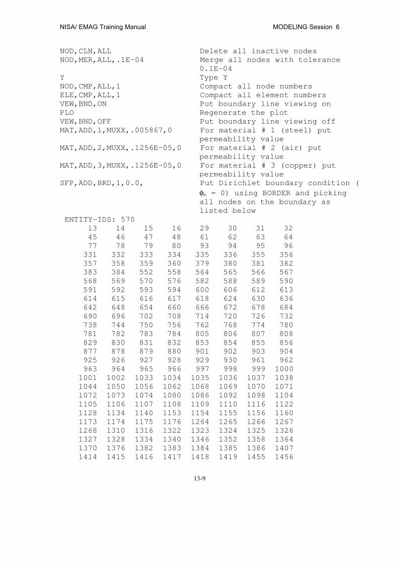
8/12/2019 emagtm
http://slidepdf.com/reader/full/emagtm 201/246
NISA/ EMAG Training Manual MODELING Session 6
13-9
NOD,CLN,ALL Delete all inactive nodes
NOD,MER,ALL,.1E-04 Merge all nodes with tolerance
0.1E-04
Y Type Y
NOD,CMP,ALL,1 Compact all node numbers
ELE,CMP,ALL,1 Compact all element numbers
VEW,BND,ON Put boundary line viewing on
PLO Regenerate the plot
VEW,BND,OFF Put boundary line viewing off
MAT,ADD,1,MUXX,.005867,0 For material # 1 (steel) put
permeability value
MAT,ADD,2,MUXX,.1256E-05,0 For material # 2 (air) put
permeability value
MAT,ADD,3,MUXX,.1256E-05,0 For material # 3 (copper) put
permeability value
SFP,ADD,BRD,1,0.0, Put Dirichlet boundary condition (
φm = 0) using BORDER and pickingall nodes on the boundary as
listed below
ENTITY-IDS: 570
13 14 15 16 29 30 31 32
45 46 47 48 61 62 63 64
77 78 79 80 93 94 95 96
331 332 333 334 335 336 355 356
357 358 359 360 379 380 381 382
383 384 552 558 564 565 566 567
568 569 570 576 582 588 589 590
591 592 593 594 600 606 612 613
614 615 616 617 618 624 630 636642 648 654 660 666 672 678 684
690 696 702 708 714 720 726 732
738 744 750 756 762 768 774 780
781 782 783 784 805 806 807 808
829 830 831 832 853 854 855 856
877 878 879 880 901 902 903 904
925 926 927 928 929 930 961 962
963 964 965 966 997 998 999 1000
1001 1002 1033 1034 1035 1036 1037 1038
1044 1050 1056 1062 1068 1069 1070 1071
1072 1073 1074 1080 1086 1092 1098 11041105 1106 1107 1108 1109 1110 1116 1122
1128 1134 1140 1153 1154 1155 1156 1160
1173 1174 1175 1176 1264 1265 1266 1267
1268 1310 1316 1322 1323 1324 1325 1326
1327 1328 1334 1340 1346 1352 1358 1364
1370 1376 1382 1383 1384 1385 1386 1407
1414 1415 1416 1417 1418 1419 1455 1456

8/12/2019 emagtm
http://slidepdf.com/reader/full/emagtm 202/246
MODELING Session 6 NIISA/ EMAG Training Manual
13-10
1457 1473 1474 1475 1476 1477 1478 1484
1490 1496 1502 1508 1521 1522 1523 1524
1537 1538 1539 1540 1553 1554 1555 1556
1569 1570 1571 1572 1585 1586 1587 1588
1601 1602 1603 1604 1617 1618 1619 1620
1633 1634 1635 1636 1649 1650 1651 1652
1665 1666 1667 1668 1681 1682 1683 1684
1697 1698 1699 1700 2151 2152 2153 2154
2155 2156 2175 2176 2177 2178 2179 2180
2199 2200 2201 2202 2203 2204 2223 2224
2225 2226 2227 2228 2247 2248 2249 2250
2251 2252 2271 2272 2273 2274 2275 2276
2618 2624 2630 2631 2632 2633 2634 2635
2636 2642 2648 2654 2655 2656 2657 2658
2659 2660 2666 2672 2678 2679 2680 2681
2682 2683 2684 2690 2696 2702 2703 2704
2705 2706 2707 2708 2714 2720 2726 2727
2728 2729 2730 2731 2732 2738 2744 2750
2751 2752 2753 2754 2755 2756 2762 2768
2774 2780 2786 2792 2798 2804 2810 2816
2822 2828 2834 2840 2846 2852 2858 2864
2870 2876 2882 2888 2894 2900 2906 2912
2918 2924 2930 2936 2942 2948 2954 2960
2966 2972 2978 2984 2990 2996 3002 3008
3014 3020 3026 3032 3038 3044 3050 3056
3062 3068 3074 3080 3081 3082 3083 3084
3105 3106 3107 3108 3129 3130 3131 3132
3153 3154 3155 3156 3177 3178 3179 3180
3201 3202 3203 3204 3225 3226 3227 32283249 3250 3251 3252 3273 3274 3275 3276
3297 3298 3299 3300 3321 3322 3323 3324
3345 3346 3347 3348 3369 3375 3381 3387
3393 3399 3405 3406 3407 3408 3409 3435
3436 3437 3438 3439 3465 3466 3467 3468
3469 3495 3496 3497 3498 3499 3525 3526
3527 3528 3529 3555 3556 3557 3558 3559
3585 3586 3587 3588 3589 3590 3596 3602
3608 3614 3620 3621 3622 3623 3624 3625
3626 3632 3638 3644 3650 3656 3657 3658
3659 3660 3661 3662 3668 3674 3680 36863692 3693 3694 3695 3696 3697 3698 3704
3710 3716 3722 3728 3729 3730 3731 3732
3733 3734 3740 3746 3752 3758 3764 3765
3766 3767 3768 3769 3770 3776 3782 3788
3794 3800
VEW,LEFT
SFP,ADD,BOX,1,0.0, Put Dirichlet boundary condition (
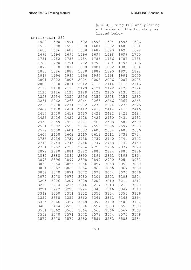
8/12/2019 emagtm
http://slidepdf.com/reader/full/emagtm 203/246
NISA/ EMAG Training Manual MODELING Session 6
13-11
φm = 0) using BOX and pickingall nodes on the boundary as
listed below
ENTITY-IDS: 380
1589 1590 1591 1592 1593 1594 1595 1596
1597 1598 1599 1600 1601 1602 1603 16041685 1686 1687 1688 1689 1690 1691 1692
1693 1694 1695 1696 1697 1698 1699 1700
1781 1782 1783 1784 1785 1786 1787 1788
1789 1790 1791 1792 1793 1794 1795 1796
1877 1878 1879 1880 1881 1882 1883 1884
1885 1886 1887 1888 1889 1890 1891 1892
1993 1994 1995 1996 1997 1998 1999 2000
2001 2002 2003 2004 2005 2006 2007 2008
2009 2010 2011 2012 2113 2114 2115 2116
2117 2118 2119 2120 2121 2122 2123 2124
2125 2126 2127 2128 2129 2130 2131 2132
2253 2254 2255 2256 2257 2258 2259 2260
2261 2262 2263 2264 2265 2266 2267 2268
2269 2270 2271 2272 2273 2274 2275 2276
2409 2410 2411 2412 2413 2414 2415 2416
2417 2418 2419 2420 2421 2422 2423 2424
2425 2426 2427 2428 2429 2430 2431 2432
2458 2459 2460 2461 2462 2588 2589 2590
2591 2592 2593 2594 2595 2596 2597 2598
2599 2600 2601 2602 2603 2604 2605 2606
2607 2608 2609 2610 2611 2612 2733 2734
2735 2736 2737 2738 2739 2740 2741 2742
2743 2744 2745 2746 2747 2748 2749 27502751 2752 2753 2754 2755 2756 2877 2878
2879 2880 2881 2882 2883 2884 2885 2886
2887 2888 2889 2890 2891 2892 2893 2894
2895 2896 2897 2898 2899 2900 3051 3052
3053 3054 3055 3056 3057 3058 3059 3060
3061 3062 3063 3064 3065 3066 3067 3068
3069 3070 3071 3072 3073 3074 3075 3076
3077 3078 3079 3080 3201 3202 3203 3204
3205 3206 3207 3208 3209 3210 3211 3212
3213 3214 3215 3216 3217 3218 3219 3220
3221 3222 3223 3224 3345 3346 3347 33483349 3350 3351 3352 3353 3354 3355 3356
3357 3358 3359 3360 3361 3362 3363 3364
3365 3366 3367 3368 3399 3400 3401 3402
3403 3404 3555 3556 3557 3558 3559 3560
3561 3562 3563 3564 3565 3566 3567 3568
3569 3570 3571 3572 3573 3574 3575 3576
3577 3578 3579 3580 3581 3582 3583 3584

8/12/2019 emagtm
http://slidepdf.com/reader/full/emagtm 204/246
MODELING Session 6 NIISA/ EMAG Training Manual
13-12
3765 3766 3767 3768 3769 3770 3771 3772
3773 3774 3775 3776 3777 3778 3779 3780
3781 3782 3783 3784 3785 3786 3787 3788
3789 3790 3791 3792 3793 3794 3795 3796
3797 3798 3799 3800
YG
VEW,TOP View along XY plane looking
through Z axis
ELE,ERA,MAT/1T2 Erase all elements of material 1 &
2
PLO,ACT Plot all active entities
VEW,TOP View along XY plane looking
through Z axis
CRD,ADD,BOX,2,0/0/-1.0E6/0/0,
Put source current density ( Jz
= -1.0E6) using BOX and picking
elements on the coil as listed
below.
ENTITY-IDS: 9
223 224 225 226 227 228 694 695
696
CRD,ADD,BOX,2,-1.0E6/0/0/0/0,
Put source current density ( Jx
= -1.0E6) using BOX and picking
elements on the coil as listed
below.
ENTITY-IDS: 9
685 686 687 688 689 690 691 692
693NFORM Use NISA DATA FORMS → NISA FORM.
Then do the following :
1.Select MFIELD.
a. Then select EMAG CONTROL, and save it
b. Select TITLE, enter title and save it
2.Select EXECUTIVE → MFIELD, select SUBA → MGSS and enter
filename for post file.
WRI NIS TRANS3D.NIS Save NISA file in TRANS3D.NIS
END End the DISPLAY III session
This completes the pre-processing (or modeling) phase of the problem.
Now you should use a text editor to edit TRANS3D.NIS file (or you can use editor availableinside DISPLAY III, as shown in modeling session 1). You can edit this file if the EXECUTIVEcards are not correct. You have to enter the CURSYM card in NISA file because it cannot beentered in DISPLAY III. First, enter *CURSYM after the *CURDEN cards. Since you have

8/12/2019 emagtm
http://slidepdf.com/reader/full/emagtm 205/246
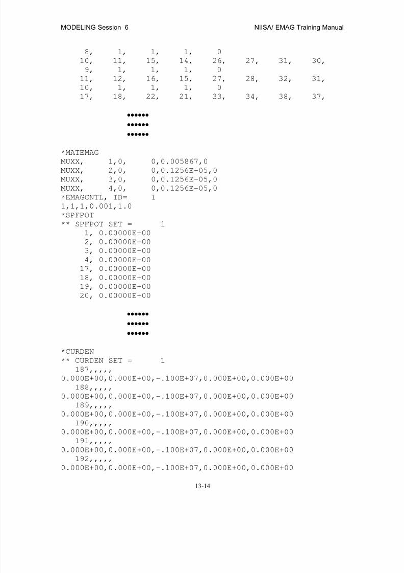
8/12/2019 emagtm
http://slidepdf.com/reader/full/emagtm 206/246
MODELING Session 6 NIISA/ EMAG Training Manual
13-14
8, 1, 1, 1, 0
10, 11, 15, 14, 26, 27, 31, 30,
9, 1, 1, 1, 0
11, 12, 16, 15, 27, 28, 32, 31,
10, 1, 1, 1, 0
17, 18, 22, 21, 33, 34, 38, 37,
•••••• ••••••
••••••
*MATEMAG
MUXX, 1,0, 0,0.005867,0
MUXX, 2,0, 0,0.1256E-05,0
MUXX, 3,0, 0,0.1256E-05,0
MUXX, 4,0, 0,0.1256E-05,0
*EMAGCNTL, ID= 11,1,1,0.001,1.0
*SPFPOT
** SPFPOT SET = 1
1, 0.00000E+00
2, 0.00000E+00
3, 0.00000E+00
4, 0.00000E+00
17, 0.00000E+00
18, 0.00000E+00
19, 0.00000E+00
20, 0.00000E+00
•••••• ••••••
••••••
*CURDEN
** CURDEN SET = 1
187,,,,,
0.000E+00,0.000E+00,-.100E+07,0.000E+00,0.000E+00
188,,,,,
0.000E+00,0.000E+00,-.100E+07,0.000E+00,0.000E+00
189,,,,,
0.000E+00,0.000E+00,-.100E+07,0.000E+00,0.000E+00
190,,,,,
0.000E+00,0.000E+00,-.100E+07,0.000E+00,0.000E+00
191,,,,,
0.000E+00,0.000E+00,-.100E+07,0.000E+00,0.000E+00
192,,,,,
0.000E+00,0.000E+00,-.100E+07,0.000E+00,0.000E+00
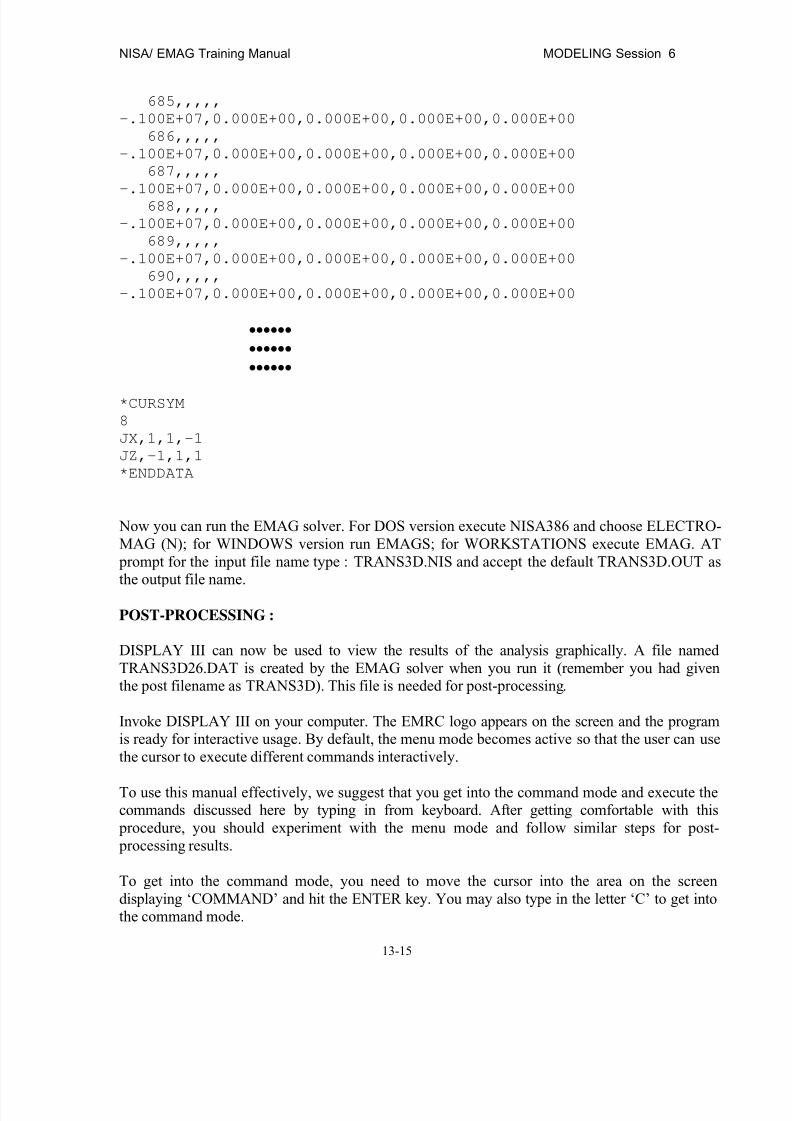
8/12/2019 emagtm
http://slidepdf.com/reader/full/emagtm 207/246
NISA/ EMAG Training Manual MODELING Session 6
13-15
685,,,,,
-.100E+07,0.000E+00,0.000E+00,0.000E+00,0.000E+00
686,,,,,
-.100E+07,0.000E+00,0.000E+00,0.000E+00,0.000E+00
687,,,,,
-.100E+07,0.000E+00,0.000E+00,0.000E+00,0.000E+00
688,,,,,
-.100E+07,0.000E+00,0.000E+00,0.000E+00,0.000E+00
689,,,,,
-.100E+07,0.000E+00,0.000E+00,0.000E+00,0.000E+00
690,,,,,
-.100E+07,0.000E+00,0.000E+00,0.000E+00,0.000E+00
•••••• •••••• ••••••
*CURSYM
8
JX,1,1,-1
JZ,-1,1,1
*ENDDATA
Now you can run the EMAG solver. For DOS version execute NISA386 and choose ELECTRO-MAG (N); for WINDOWS version run EMAGS; for WORKSTATIONS execute EMAG. AT prompt for the input file name type : TRANS3D.NIS and accept the default TRANS3D.OUT asthe output file name.
POST-PROCESSING :
DISPLAY III can now be used to view the results of the analysis graphically. A file namedTRANS3D26.DAT is created by the EMAG solver when you run it (remember you had giventhe post filename as TRANS3D). This file is needed for post-processing.
Invoke DISPLAY III on your computer. The EMRC logo appears on the screen and the programis ready for interactive usage. By default, the menu mode becomes active so that the user can usethe cursor to execute different commands interactively.
To use this manual effectively, we suggest that you get into the command mode and execute thecommands discussed here by typing in from keyboard. After getting comfortable with this procedure, you should experiment with the menu mode and follow similar steps for post- processing results.
To get into the command mode, you need to move the cursor into the area on the screendisplaying ‘COMMAND’ and hit the ENTER key. You may also type in the letter ‘C’ to get intothe command mode.
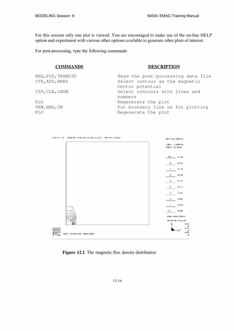
8/12/2019 emagtm
http://slidepdf.com/reader/full/emagtm 208/246
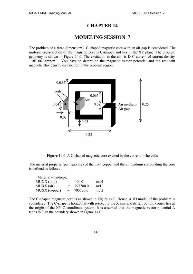
8/12/2019 emagtm
http://slidepdf.com/reader/full/emagtm 209/246
NISA/ EMAG Training Manual MODELING Session 7
14-1
CHAPTER 14
MODELING SESSION 7
The problem of a three dimensional C-shaped magnetic core with an air gap is considered. Theuniform cross-section of the magnetic core is C-shaped and lies in the XY plane. The problemgeometry is shown in Figure 14.0. The excitation in the coil is D C current of current density1.0E+06 Amp/m2 . You have to determine the magnetic vector potential and the resultantmagnetic flux density distribution in the problem region .
0.05
coils
0.065Air
0.04 0.02 Air medium 0.25Air gap
0.020.05
0.25
Figure 14.0 A C-shaped magnetic core excited by the current in the coils
The material property (permeability) of the iron, copper and the air medium surrounding the coreis defined as follows :
Material = IsotropicMUXX (iron) = 400.0 m/HMUXX (air) = 795780.0 m/H
MUXX (copper) = 795780.0 m/H
The C-shaped magnetic core is as shown in Figure 14.0. Hence, a 3D model of the problem isconsidered. The C-shape is horizontal with respect to the X axis and its left bottom corner lies atthe origin of the XY Z coordinate system. It is assumed that the magnetic vector potential Atends to 0 on the boundary shown in Figure 14.0.

8/12/2019 emagtm
http://slidepdf.com/reader/full/emagtm 210/246
MODELING Session 7 NIISA/ EMAG Training Manual
14-2
Since the geometry of the C-shaped magnetic core model is in 3D, therefore 3D Hexahedralelement is chosen. NISA offers one of the most complete element libraries among commercialsoftwares, and a list of currently available elements can be found in the User’s manual.
The first step in modeling this problem is to create the geometry of C-shaped magnetic core interms of lines as shown in Figures 14.0. The lines are created by joining grids (points in spacewith predefined coordinates). These lines are used to create surfaces called patches. The patchesare used to create hyperpatches. Once the geometry is obtained in terms of hyperpatches, meshgeneration is used and the mesh is created. Then, excitation (i.e., current density) and the boundary conditions along with material and geometric properties are defined for the elements.Furthermore, analysis and sub analysis types are defined at this stage. Finally, at the end ofmodeling a NISA ASCII file is obtained to perform a Magnetostatic analysis using magneticvector potential.
Invoke DISPLAY III on your computer. When the screen appears click mouse on the COM HOT button ( or hit key ‘c’ on the keyboard ) to get into the command mode. Now enter the followingcommands interactively to generate the model.
COMMANDS DESCRIPTION
SET,TOLC,.1E-04 Since the dimensions are of order
SET,TOLD,.1E-04 or 0.01 or less set the PICK and
DIST tolerance to 100 times less
GRD,ADD,1,0.0/0.0/0.0 Create grid at the origin of the
global coordinate system (0/0/0)
GRD,ADD,2,0.05/0.0/0.0 Create grid # 2 at (0.05/0/0)
GRD,ADD,3,0.07/0.0/0.0 Create grid # 3 at (0.07/0/0)
GRD,ADD,4,0.18/0.0/0.0 Create grid # 4 at (0.18/0/0)
GRD,ADD,5,0.2/0.0/0.0 Create grid # 5 at (0.2/0/0)
GRD,ADD,6,0.25/0.0/0.0 Create grid # 6 at (0.25/0/0)
GRD,TRS,1T6,B7/1,0.0/0.05/0.0/0,1
Translate grids 1 through 6 by
0.05 in the Y direction
GRD,TRS,7T12,B13/1,0.0/0.055/0.0/0,1
Translate grids 7 through 12 by
0.055 in the Y direction
GRD,TRS,18,19,0.02/0.0/0.0/0,1Translate grids 18 by 0.02 in the
X direction
GRD,TRS,13,20,-0.02/0.0/0.0/0,1
Translate grids 13 by -0.02 in the
X direction
GRD,TRS,13T20,B21/1,0.0/0.01/0.0/0,1
Translate grids 13 through 20 by

8/12/2019 emagtm
http://slidepdf.com/reader/full/emagtm 211/246
NISA/ EMAG Training Manual MODELING Session 7
14-3
0.01 in the Y direction
GRD,MIR,1T28,B29/1,Y0.125 Mirror grids 1 to 28 about the XZ
plane at Y = 0.125
LIN,2GD,1,2,1 Join grids 1, 2 to create line # 1
LIN,2GD,2,3,2 Join grids 2, 3 to create line # 2
LIN,2GD,3,4,3 Join grids 3, 4 to create line # 3
LIN,2GD,4,5,4 Join grids 4, 5 to create line # 4
LIN,2GD,5,6,5 Join grids 5, 6 to create line # 5
LIN,2GD,7,8,6 Join grids 7, 8 to create line # 6
LIN,2GD,8,9,7 Join grids 8, 9 to create line # 7
LIN,2GD,9,10,8 Join grids 9,10 to create line # 8
LIN,2GD,10,11,9 Join grids 10,11 to create line #9
LIN,2GD,11,12,10 Join grids 11, 12 to create line
#10
LIN,2GD,20,13,11 Join grids 20, 13 to create line #
11
LIN,2GD,13,14,12 Join grids 13, 14 to create line #
12
LIN,2GD,14,15,13 Join grids 14, 15 to create line #
13
LIN,2GD,15,16,14 Join grids 15, 16 to create line #
14
LIN,2GD,16,17,15 Join grids 16, 17 to create line #
15
LIN,2GD,17,18,16 Join grids 17, 18 to create line #
16
LIN,2GD,18,19,17 Join grids 18, 19 to create line #
17
LIN,2GD,28,21,18 Join grids 28, 21 to create line #18
LIN,2GD,21,22,19 Join grids 21, 22 to create line #
19
LIN,2GD,22,23,20 Join grids 22, 23 to create line #
20
LIN,2GD,23,24,21 Join grids 23, 24 to create line #
21
LIN,2GD,24,25,22 Join grids 24, 25 to create line #
22
LIN,2GD,25,26,23 Join grids 25, 26 to create line #
23LIN,2GD,26,27,24 Join grids 26, 27 to create line #
24
LIN,MIR,1T24,B27/1,Y0.125 Mirror lines 1 through 24 about XZ
plane at Y = 0.125
PAT,2LN,6,1,1 Use lines 6 and 1 to create patch
# 1
PAT,2LN,7,2,2 Use lines 7 and 2 to create patch

8/12/2019 emagtm
http://slidepdf.com/reader/full/emagtm 212/246
MODELING Session 7 NIISA/ EMAG Training Manual
14-4
# 2
PAT,2LN,8,3,3 Use lines 8 and 3 to create patch
# 3
PAT,2LN,9,4,4 Use lines 9 and 4 to create patch
# 4
PAT,2LN,10,5,5 Use lines 10 and 5 to create patch
# 5
PAT,2LN,12,6,6 Use lines 12 and 6 to create patch
# 6
PAT,2LN,13,7,7 Use lines 13 and 7 to create patch
# 7
PAT,2LN,14,8,8 Use lines 14 and 8 to create patch
# 8
PAT,2LN,15,9,9 Use lines 15 and 9 to create patch
# 9
PAT,2LN,16,10,10 Use lines 16 and 10 to create
patch # 10
PAT,2LN,18,11,11 Use lines 18 and 11 to create
patch # 11
PAT,2LN,19,12,12 Use lines 19 and 12 to create
patch # 12
PAT,2LN,20,13,13 Use lines 20 and 13 to create
patch # 13
PAT,2LN,21,14,14 Use lines 21 and 14 to create
patch # 14
PAT,2LN,22,15,15 Use lines 22 and 15 to create
patch # 15
PAT,2LN,23,16,16 Use lines 23 and 16 to create
patch # 16PAT,2LN,24,17,17 Use lines 24 and 17 to create
patch # 17
PAT,2LN,44,18,18 Use lines 44 and 18 to create
patch # 18
PAT,2LN,45,19,19 Use lines 45 and 19 to create
patch # 19
PAT,2LN,46,20,20 Use lines 46 and 20 to create
patch # 20
PAT,2LN,47,21,21 Use lines 47 and 21 to create
patch # 21
PAT,2LN,48,22,22 Use lines 48 and 22 to createpatch # 22
PAT,2LN,49,23,23 Use lines 49 and 23 to create
patch # 23
PAT,2LN,50,24,24 Use lines 50 and 24 to create
patch # 24
PAT,MIR,1T17,B25/1,Y0.125 Mirror patches 1 through 17 about
the XZ plane at Y = 0.125
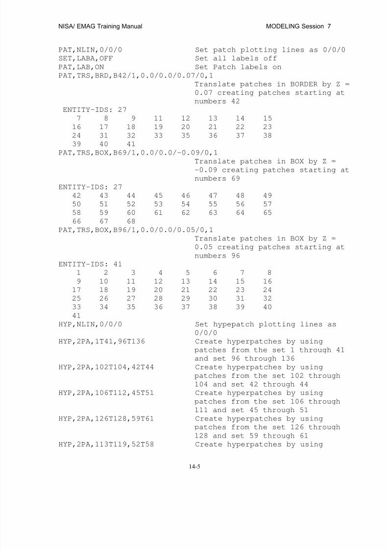
8/12/2019 emagtm
http://slidepdf.com/reader/full/emagtm 213/246
NISA/ EMAG Training Manual MODELING Session 7
14-5
PAT,NLIN,0/0/0 Set patch plotting lines as 0/0/0
SET,LABA,OFF Set all labels off
PAT,LAB,ON Set Patch labels on
PAT,TRS,BRD,B42/1,0.0/0.0/0.07/0,1
Translate patches in BORDER by Z =
0.07 creating patches starting at
numbers 42
ENTITY-IDS: 27
7 8 9 11 12 13 14 15
16 17 18 19 20 21 22 23
24 31 32 33 35 36 37 38
39 40 41
PAT,TRS,BOX,B69/1,0.0/0.0/-0.09/0,1
Translate patches in BOX by Z =
-0.09 creating patches starting at
numbers 69
ENTITY-IDS: 27
42 43 44 45 46 47 48 49
50 51 52 53 54 55 56 57
58 59 60 61 62 63 64 65
66 67 68
PAT,TRS,BOX,B96/1,0.0/0.0/0.05/0,1
Translate patches in BOX by Z =
0.05 creating patches starting at
numbers 96
ENTITY-IDS: 41
1 2 3 4 5 6 7 8
9 10 11 12 13 14 15 16
17 18 19 20 21 22 23 2425 26 27 28 29 30 31 32
33 34 35 36 37 38 39 40
41
HYP,NLIN,0/0/0 Set hypepatch plotting lines as
0/0/0
HYP,2PA,1T41,96T136 Create hyperpatches by using
patches from the set 1 through 41
and set 96 through 136
HYP,2PA,102T104,42T44 Create hyperpatches by using
patches from the set 102 through
104 and set 42 through 44HYP,2PA,106T112,45T51 Create hyperpatches by using
patches from the set 106 through
111 and set 45 through 51
HYP,2PA,126T128,59T61 Create hyperpatches by using
patches from the set 126 through
128 and set 59 through 61
HYP,2PA,113T119,52T58 Create hyperpatches by using
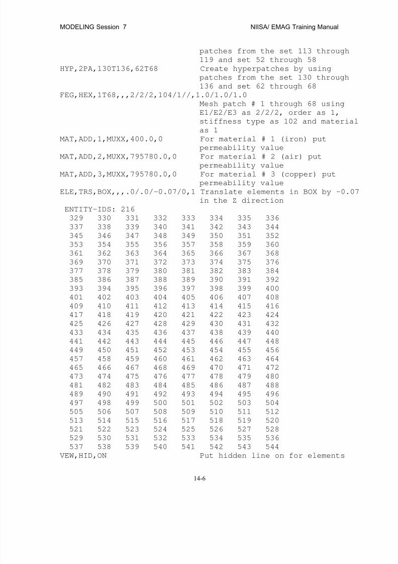
8/12/2019 emagtm
http://slidepdf.com/reader/full/emagtm 214/246
MODELING Session 7 NIISA/ EMAG Training Manual
14-6
patches from the set 113 through
119 and set 52 through 58
HYP,2PA,130T136,62T68 Create hyperpatches by using
patches from the set 130 through
136 and set 62 through 68
FEG,HEX,1T68,,,2/2/2,104/1//,1.0/1.0/1.0
Mesh patch # 1 through 68 using
E1/E2/E3 as 2/2/2, order as 1,
stiffness type as 102 and material
as 1
MAT,ADD,1,MUXX,400.0,0 For material # 1 (iron) put
permeability value
MAT,ADD,2,MUXX,795780.0,0 For material # 2 (air) put
permeability value
MAT,ADD,3,MUXX,795780.0,0 For material # 3 (copper) put
permeability value
ELE,TRS,BOX,,,.0/.0/-0.07/0,1 Translate elements in BOX by –0.07
in the Z direction
ENTITY-IDS: 216
329 330 331 332 333 334 335 336
337 338 339 340 341 342 343 344
345 346 347 348 349 350 351 352
353 354 355 356 357 358 359 360
361 362 363 364 365 366 367 368
369 370 371 372 373 374 375 376
377 378 379 380 381 382 383 384
385 386 387 388 389 390 391 392
393 394 395 396 397 398 399 400
401 402 403 404 405 406 407 408409 410 411 412 413 414 415 416
417 418 419 420 421 422 423 424
425 426 427 428 429 430 431 432
433 434 435 436 437 438 439 440
441 442 443 444 445 446 447 448
449 450 451 452 453 454 455 456
457 458 459 460 461 462 463 464
465 466 467 468 469 470 471 472
473 474 475 476 477 478 479 480
481 482 483 484 485 486 487 488
489 490 491 492 493 494 495 496497 498 499 500 501 502 503 504
505 506 507 508 509 510 511 512
513 514 515 516 517 518 519 520
521 522 523 524 525 526 527 528
529 530 531 532 533 534 535 536
537 538 539 540 541 542 543 544
VEW,HID,ON Put hidden line on for elements
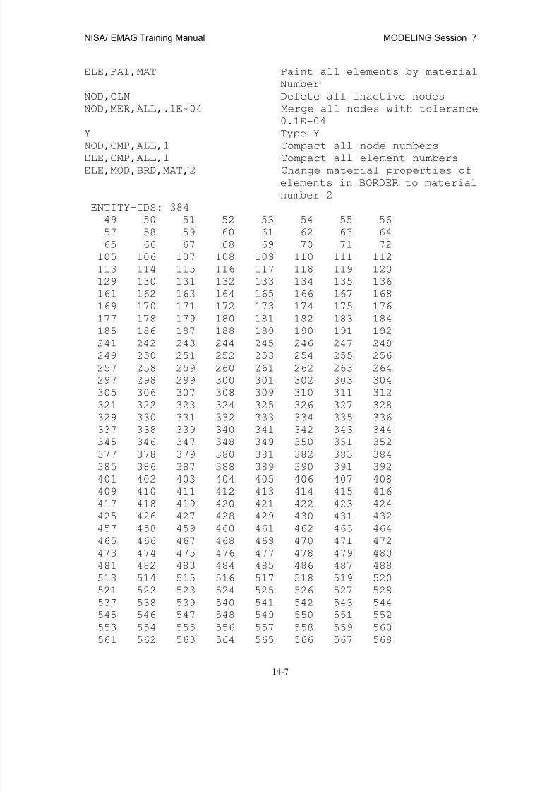
8/12/2019 emagtm
http://slidepdf.com/reader/full/emagtm 215/246
NISA/ EMAG Training Manual MODELING Session 7
14-7
ELE,PAI,MAT Paint all elements by material
Number
NOD,CLN Delete all inactive nodes
NOD,MER,ALL,.1E-04 Merge all nodes with tolerance
0.1E-04
Y Type Y
NOD,CMP,ALL,1 Compact all node numbers
ELE,CMP,ALL,1 Compact all element numbers
ELE,MOD,BRD,MAT,2 Change material properties of
elements in BORDER to material
number 2
ENTITY-IDS: 384
49 50 51 52 53 54 55 56
57 58 59 60 61 62 63 64
65 66 67 68 69 70 71 72
105 106 107 108 109 110 111 112
113 114 115 116 117 118 119 120
129 130 131 132 133 134 135 136
161 162 163 164 165 166 167 168
169 170 171 172 173 174 175 176
177 178 179 180 181 182 183 184
185 186 187 188 189 190 191 192
241 242 243 244 245 246 247 248
249 250 251 252 253 254 255 256
257 258 259 260 261 262 263 264
297 298 299 300 301 302 303 304
305 306 307 308 309 310 311 312
321 322 323 324 325 326 327 328
329 330 331 332 333 334 335 336337 338 339 340 341 342 343 344
345 346 347 348 349 350 351 352
377 378 379 380 381 382 383 384
385 386 387 388 389 390 391 392
401 402 403 404 405 406 407 408
409 410 411 412 413 414 415 416
417 418 419 420 421 422 423 424
425 426 427 428 429 430 431 432
457 458 459 460 461 462 463 464
465 466 467 468 469 470 471 472
473 474 475 476 477 478 479 480481 482 483 484 485 486 487 488
513 514 515 516 517 518 519 520
521 522 523 524 525 526 527 528
537 538 539 540 541 542 543 544
545 546 547 548 549 550 551 552
553 554 555 556 557 558 559 560
561 562 563 564 565 566 567 568
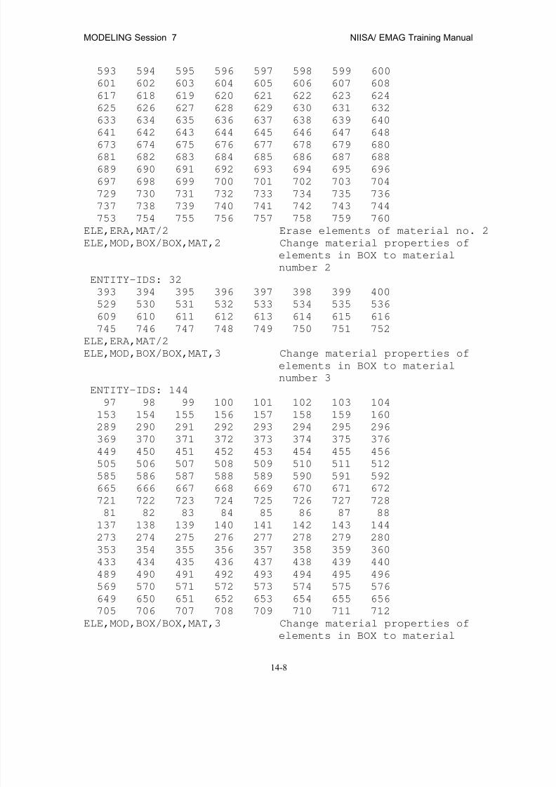
8/12/2019 emagtm
http://slidepdf.com/reader/full/emagtm 216/246
MODELING Session 7 NIISA/ EMAG Training Manual
14-8
593 594 595 596 597 598 599 600
601 602 603 604 605 606 607 608
617 618 619 620 621 622 623 624
625 626 627 628 629 630 631 632
633 634 635 636 637 638 639 640
641 642 643 644 645 646 647 648
673 674 675 676 677 678 679 680
681 682 683 684 685 686 687 688
689 690 691 692 693 694 695 696
697 698 699 700 701 702 703 704
729 730 731 732 733 734 735 736
737 738 739 740 741 742 743 744
753 754 755 756 757 758 759 760
ELE,ERA,MAT/2 Erase elements of material no. 2
ELE,MOD,BOX/BOX,MAT,2 Change material properties of
elements in BOX to material
number 2
ENTITY-IDS: 32
393 394 395 396 397 398 399 400
529 530 531 532 533 534 535 536
609 610 611 612 613 614 615 616
745 746 747 748 749 750 751 752
ELE,ERA,MAT/2
ELE,MOD,BOX/BOX,MAT,3 Change material properties of
elements in BOX to material
number 3
ENTITY-IDS: 144
97 98 99 100 101 102 103 104
153 154 155 156 157 158 159 160289 290 291 292 293 294 295 296
369 370 371 372 373 374 375 376
449 450 451 452 453 454 455 456
505 506 507 508 509 510 511 512
585 586 587 588 589 590 591 592
665 666 667 668 669 670 671 672
721 722 723 724 725 726 727 728
81 82 83 84 85 86 87 88
137 138 139 140 141 142 143 144
273 274 275 276 277 278 279 280
353 354 355 356 357 358 359 360433 434 435 436 437 438 439 440
489 490 491 492 493 494 495 496
569 570 571 572 573 574 575 576
649 650 651 652 653 654 655 656
705 706 707 708 709 710 711 712
ELE,MOD,BOX/BOX,MAT,3 Change material properties of
elements in BOX to material
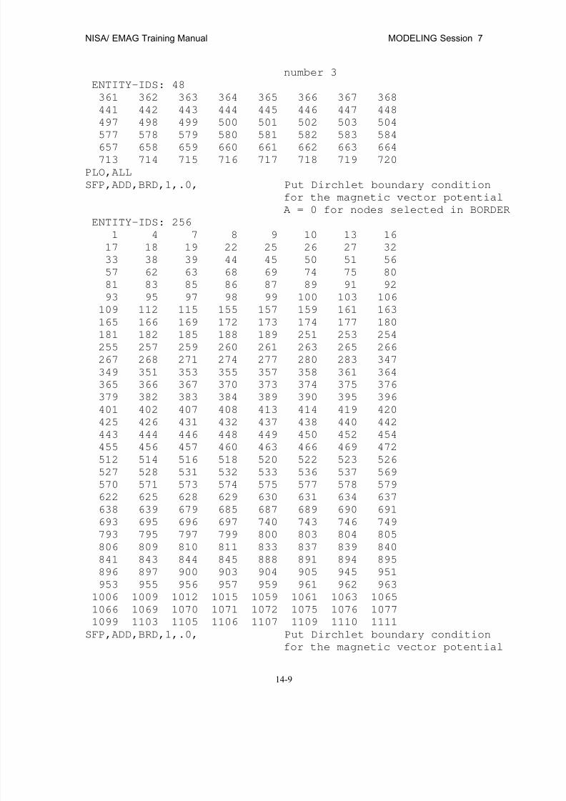
8/12/2019 emagtm
http://slidepdf.com/reader/full/emagtm 217/246

8/12/2019 emagtm
http://slidepdf.com/reader/full/emagtm 218/246

8/12/2019 emagtm
http://slidepdf.com/reader/full/emagtm 219/246
NISA/ EMAG Training Manual MODELING Session 7
14-11
951 958 959 960 961 962 963 964
965 966 967 968 969 970 971 972
979 980 981 982 983 984 985 986
987 992 993 994 995 996 997 998
999 1004 1005 1012 1013 1014 1015 1016
1017 1022 1023 1024 1025 1030 1031 1032
1033 1038 1039 1040 1041 1046 1047 1048
1049 1054 1055 1056 1057 1062 1063 1064
1065 1066 1067 1068 1069 1070 1071 1078
1079 1080 1084 1085 1088 1089 1092 1093
1096 1097 1098 1099 1104 1105 1106 1107
YG
SFP,SIZ,.005 Select symbol size for SPFPOT as
0.05
CRD,ADD,BOX,2,1E6/0/0/0/0, Put current density in X direction
as 1.0E+06 for elements in BOX
ENTITY-IDS: 72
353 354 355 356 357 358 359 360
361 362 363 364 365 366 367 368
369 370 371 372 373 374 375 376
433 434 435 436 437 438 439 440
441 442 443 444 445 446 447 448
449 450 451 452 453 454 455 456
489 490 491 492 493 494 495 496
497 498 499 500 501 502 503 504
505 506 507 508 509 510 511 512
CRD,ADD,BOX,2,-1E6/0/0/0/0, Put current density in X direction
as -1.0E+06 for elements in BOX
ENTITY-IDS: 72569 570 571 572 573 574 575 576
577 578 579 580 581 582 583 584
585 586 587 588 589 590 591 592
649 650 651 652 653 654 655 656
657 658 659 660 661 662 663 664
665 666 667 668 669 670 671 672
705 706 707 708 709 710 711 712
713 714 715 716 717 718 719 720
721 722 723 724 725 726 727 728
CRD,ADD,BOX,2,0/0/1E6/0/0, Put current density in Z direction
as 1.0E+06 for elements in BOXENTITY-IDS: 24
81 82 83 84 85 86 87 88
137 138 139 140 141 142 143 144
273 274 275 276 277 278 279 280
CRD,ADD,BOX,2,0/0/-1E6/0/0, Put current density in X direction
as -1.0E+06 for elements in BOX
ENTITY-IDS: 24

8/12/2019 emagtm
http://slidepdf.com/reader/full/emagtm 220/246

8/12/2019 emagtm
http://slidepdf.com/reader/full/emagtm 221/246
NISA/ EMAG Training Manual MODELING Session 7
14-13
7,,,, 1.80000E-01, 2.50000E-01, 2.50000E-02, 0
8,,,, 1.80000E-01, 2.25000E-01, 2.50000E-02, 0
9,,,, 1.80000E-01, 2.00000E-01, 2.50000E-02, 0
10,,,, 2.00000E-01, 2.50000E-01, 2.50000E-02, 0
••••••
••••••
••••••
*ELEMENTS
1, 1, 1, 1, 0
1, 2, 5, 4, 7, 8, 11, 10,
2, 1, 1, 1, 0
2, 3, 6, 5, 8, 9, 12, 11,
3, 1, 1, 1, 0
7, 8, 11, 10, 13, 14, 17, 16,
4, 1, 1, 1, 0
8, 9, 12, 11, 14, 15, 18, 17,
5, 1, 1, 1, 0
19, 20, 23, 22, 28, 29, 32, 31,
6, 1, 1, 1, 0
20, 18, 17, 23, 29, 12, 11, 32,
7, 1, 1, 1, 0
22, 23, 26, 25, 31, 32, 35, 34,
8, 1, 1, 1, 0
23, 17, 16, 26, 32, 11, 10, 35,
9, 1, 1, 1, 0
28, 29, 32, 31, 37, 38, 41, 40,
10, 1, 1, 1, 0
29, 12, 11, 32, 38, 6, 5, 41,
••••••
••••••
••••••
*MATEMAG
MUXX, 1,0, 0,400.0,0
MUXX, 2,0, 0,795780.0,0
MUXX, 3,0, 0,795780.0,0
*EMAGCNTL, ID= 1
1,1,1,0.001,1.0
*SPFPOT
** SPFPOT SET = 1
1, 0.00000E+00
2, 0.00000E+00
3, 0.00000E+00
4, 0.00000E+00
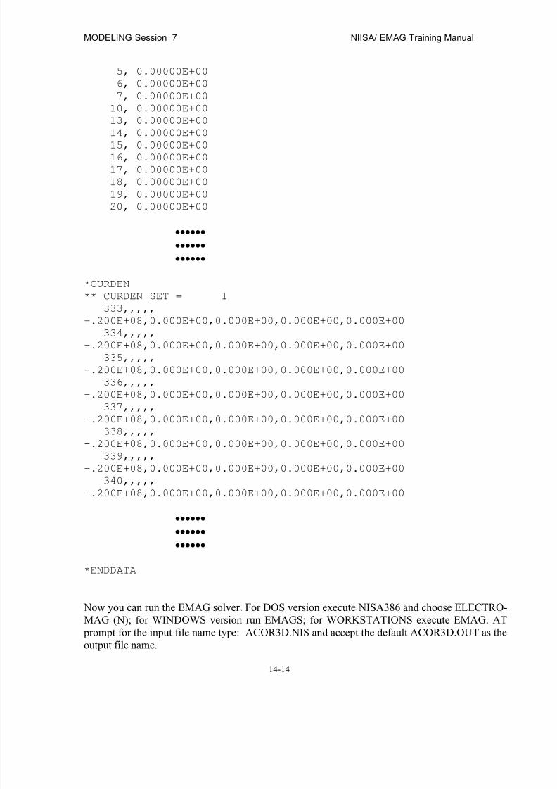
8/12/2019 emagtm
http://slidepdf.com/reader/full/emagtm 222/246
MODELING Session 7 NIISA/ EMAG Training Manual
14-14
5, 0.00000E+00
6, 0.00000E+00
7, 0.00000E+00
10, 0.00000E+00
13, 0.00000E+00
14, 0.00000E+00
15, 0.00000E+00
16, 0.00000E+00
17, 0.00000E+00
18, 0.00000E+00
19, 0.00000E+00
20, 0.00000E+00
••••••
••••••
••••••
*CURDEN
** CURDEN SET = 1
333,,,,,
-.200E+08,0.000E+00,0.000E+00,0.000E+00,0.000E+00
334,,,,,
-.200E+08,0.000E+00,0.000E+00,0.000E+00,0.000E+00
335,,,,,
-.200E+08,0.000E+00,0.000E+00,0.000E+00,0.000E+00
336,,,,,
-.200E+08,0.000E+00,0.000E+00,0.000E+00,0.000E+00
337,,,,,
-.200E+08,0.000E+00,0.000E+00,0.000E+00,0.000E+00
338,,,,,
-.200E+08,0.000E+00,0.000E+00,0.000E+00,0.000E+00
339,,,,,
-.200E+08,0.000E+00,0.000E+00,0.000E+00,0.000E+00
340,,,,,
-.200E+08,0.000E+00,0.000E+00,0.000E+00,0.000E+00
••••••
••••••
••••••
*ENDDATA
Now you can run the EMAG solver. For DOS version execute NISA386 and choose ELECTRO-MAG (N); for WINDOWS version run EMAGS; for WORKSTATIONS execute EMAG. AT prompt for the input file name type: ACOR3D.NIS and accept the default ACOR3D.OUT as theoutput file name.
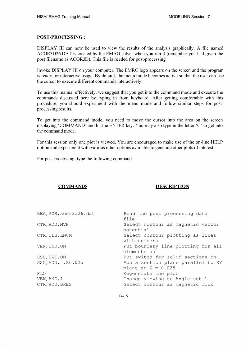
8/12/2019 emagtm
http://slidepdf.com/reader/full/emagtm 223/246
NISA/ EMAG Training Manual MODELING Session 7
14-15
POST-PROCESSING :
DISPLAY III can now be used to view the results of the analysis graphically. A file namedACOR3D26.DAT is created by the EMAG solver when you run it (remember you had given the
post filename as ACOR3D). This file is needed for post-processing.
Invoke DISPLAY III on your computer. The EMRC logo appears on the screen and the programis ready for interactive usage. By default, the menu mode becomes active so that the user can usethe cursor to execute different commands interactively.
To use this manual effectively, we suggest that you get into the command mode and execute thecommands discussed here by typing in from keyboard. After getting comfortable with this procedure, you should experiment with the menu mode and follow similar steps for post- processing results.
To get into the command mode, you need to move the cursor into the area on the screendisplaying ‘COMMAND’ and hit the ENTER key. You may also type in the letter ‘C’ to get intothe command mode.
For this session only one plot is viewed. You are encouraged to make use of the on-line HELPoption and experiment with various other options available to generate other plots of interest.
For post-processing, type the following commands
COMMANDS DESCRIPTION
REA,POS,acor3d26.dat Read the post processing data
file
CTR,ADD,MVP Select contour as magnetic vector
potential
CTR,CLB,LNUM Select contour plotting as lines
with numbers
VEW,BND,ON Put boundary line plotting for allelements on
SSC,SWI,ON Put switch for solid sections on
SSC,ADD, ,Z0.025 Add a section plane parallel to XY
plane at Z = 0.025
PLO Regenerate the plot
VEW,ANG,1 Change viewing to Angle set 1
CTR,ADD,BRES Select contour as magnetic flux
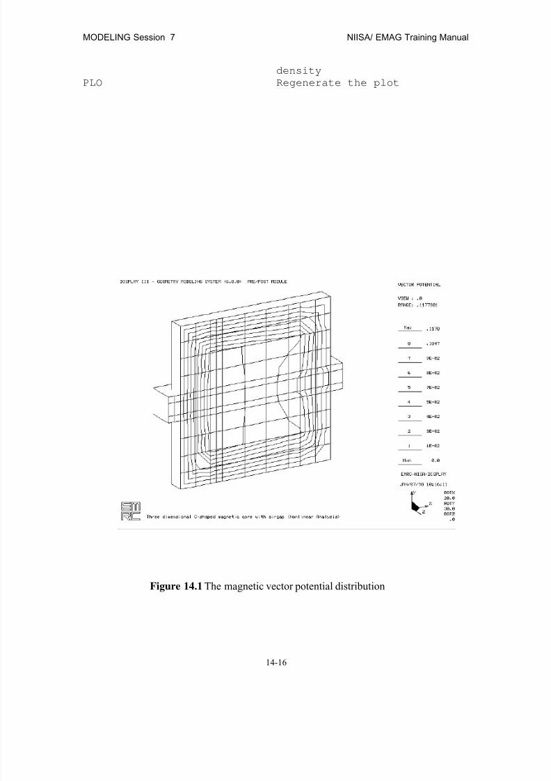
8/12/2019 emagtm
http://slidepdf.com/reader/full/emagtm 224/246
MODELING Session 7 NIISA/ EMAG Training Manual
14-16
density
PLO Regenerate the plot
Figure 14.1 The magnetic vector potential distribution
8/12/2019 emagtm
http://slidepdf.com/reader/full/emagtm 225/246
NISA/ EMAG Training Manual MODELING Session 7
14-17
Figure 14.2 The magnetic flux density distribution

8/12/2019 emagtm
http://slidepdf.com/reader/full/emagtm 226/246
MODELING Session 7 NIISA/ EMAG Training Manual
14-18
This page intentionally left blank
8/12/2019 emagtm
http://slidepdf.com/reader/full/emagtm 227/246
NISA/ EMAG Training Manual MODELING Session 8
15-1
CHAPTER 15
MODELING SESSION 8
The steel plate problem of modeling session 2 is considered here for the HEAT analysis. Heat isgenerated due to current flowing in the steel plate. The boundary of the problem is assumed to beat 0 degrees centigrade at all times. You have to determine the temperature distribution in thesteel plate and the punchout hole.
The material property (for HEAT analysis) of copper, steel and air are defined as follows:
Material = IsotropicKXX (air) = 0.024 W/moCDENS(air) = 1.29 kg/m3
C(air) = 1005.0 J/kgoC
KXX (steel) = 80.0 W/mo
CDENS(steel) = 7000.0 kg/m3
C(steel) = 470.0 J/kgoC
KXX (copper) = 398.0 W/moC
DENS(copper) = 8900.0 kg/m3
C(copper) = 4600.0 J/kgoC
Since the geometry, the finite element mesh etc. of this steel plate model is already created inmodeling session 2 the same is used here. For this use the NISA file DC4E.NIS.
Invoke DISPLAY III on your computer. When the screen appears click mouse on the COM HOT button ( or hit key ‘c’ on the keyboard ) to get into the command mode. Now enter the followingcommands interactively to generate the model.
COMMANDS DESCRIPTION
REA,NIS,DC4E.NIS Read the EMAG NISA file
SET,LABA,OFF Set all labels off
ELE,PAI,MAT Paint all elements by material
VEW,HID,OFF Put hidden line for elements on
PLO,ALL Plot all entitiesHBC,DEL,BC_DATA Delete all EMAG boundary
conditions
ENTITY-IDS: 100
466000001 12500 466000001 12515 466000001 12530
466000001 12545 466000001 12680 466000001 12695
466000001 12710 466000001 12725 466000001 12860
466000001 12875 466000001 12890 466000001 12905
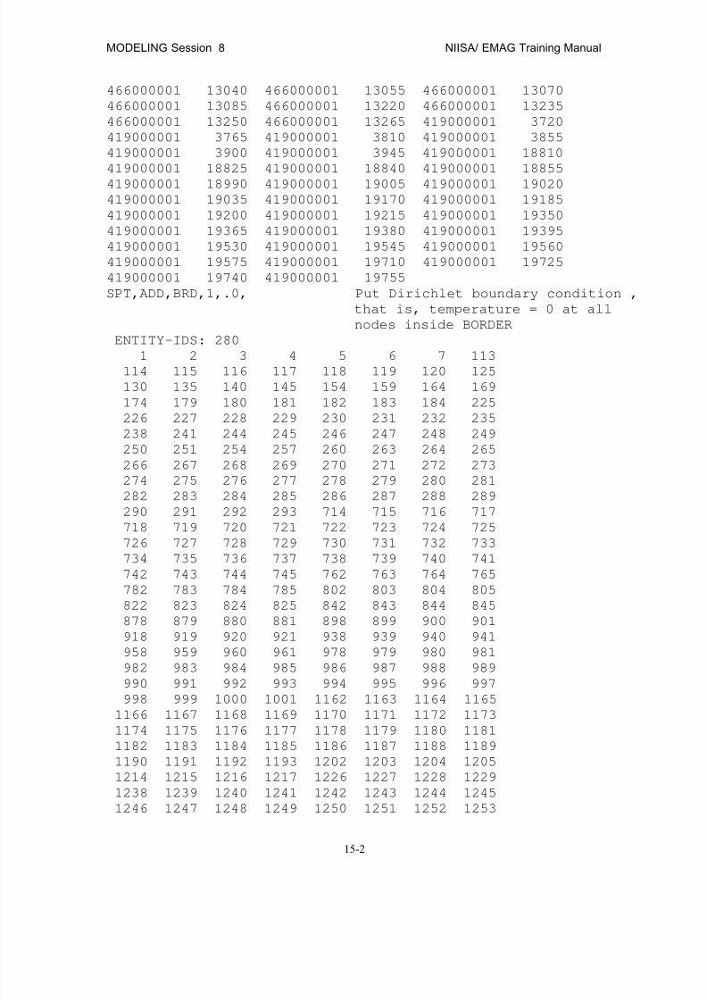
8/12/2019 emagtm
http://slidepdf.com/reader/full/emagtm 228/246
MODELING Session 8 NIISA/ EMAG Training Manual
15-2
466000001 13040 466000001 13055 466000001 13070
466000001 13085 466000001 13220 466000001 13235
466000001 13250 466000001 13265 419000001 3720
419000001 3765 419000001 3810 419000001 3855
419000001 3900 419000001 3945 419000001 18810
419000001 18825 419000001 18840 419000001 18855
419000001 18990 419000001 19005 419000001 19020
419000001 19035 419000001 19170 419000001 19185
419000001 19200 419000001 19215 419000001 19350
419000001 19365 419000001 19380 419000001 19395
419000001 19530 419000001 19545 419000001 19560
419000001 19575 419000001 19710 419000001 19725
419000001 19740 419000001 19755
SPT,ADD,BRD,1,.0, Put Dirichlet boundary condition ,
that is, temperature = 0 at all
nodes inside BORDER
ENTITY-IDS: 280
1 2 3 4 5 6 7 113
114 115 116 117 118 119 120 125
130 135 140 145 154 159 164 169
174 179 180 181 182 183 184 225
226 227 228 229 230 231 232 235
238 241 244 245 246 247 248 249
250 251 254 257 260 263 264 265
266 267 268 269 270 271 272 273
274 275 276 277 278 279 280 281
282 283 284 285 286 287 288 289
290 291 292 293 714 715 716 717
718 719 720 721 722 723 724 725726 727 728 729 730 731 732 733
734 735 736 737 738 739 740 741
742 743 744 745 762 763 764 765
782 783 784 785 802 803 804 805
822 823 824 825 842 843 844 845
878 879 880 881 898 899 900 901
918 919 920 921 938 939 940 941
958 959 960 961 978 979 980 981
982 983 984 985 986 987 988 989
990 991 992 993 994 995 996 997
998 999 1000 1001 1162 1163 1164 11651166 1167 1168 1169 1170 1171 1172 1173
1174 1175 1176 1177 1178 1179 1180 1181
1182 1183 1184 1185 1186 1187 1188 1189
1190 1191 1192 1193 1202 1203 1204 1205
1214 1215 1216 1217 1226 1227 1228 1229
1238 1239 1240 1241 1242 1243 1244 1245
1246 1247 1248 1249 1250 1251 1252 1253
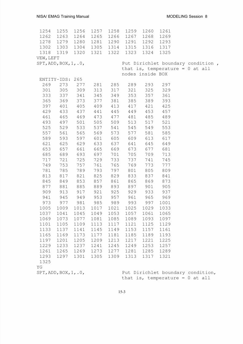
8/12/2019 emagtm
http://slidepdf.com/reader/full/emagtm 229/246
NISA/ EMAG Training Manual MODELING Session 8
15-3
1254 1255 1256 1257 1258 1259 1260 1261
1262 1263 1264 1265 1266 1267 1268 1269
1278 1279 1280 1281 1290 1291 1292 1293
1302 1303 1304 1305 1314 1315 1316 1317
1318 1319 1320 1321 1322 1323 1324 1325
VEW,LEFT
SPT,ADD,BOX,1,.0, Put Dirichlet boundary condition ,
that is, temperature = 0 at all
nodes inside BOX
ENTITY-IDS: 265
269 273 277 281 285 289 293 297
301 305 309 313 317 321 325 329
333 337 341 345 349 353 357 361
365 369 373 377 381 385 389 393
397 401 405 409 413 417 421 425
429 433 437 441 445 449 453 457
461 465 469 473 477 481 485 489
493 497 501 505 509 513 517 521
525 529 533 537 541 545 549 553
557 561 565 569 573 577 581 585
589 593 597 601 605 609 613 617
621 625 629 633 637 641 645 649
653 657 661 665 669 673 677 681
685 689 693 697 701 705 709 713
717 721 725 729 733 737 741 745
749 753 757 761 765 769 773 777
781 785 789 793 797 801 805 809
813 817 821 825 829 833 837 841
845 849 853 857 861 865 869 873877 881 885 889 893 897 901 905
909 913 917 921 925 929 933 937
941 945 949 953 957 961 965 969
973 977 981 985 989 993 997 1001
1005 1009 1013 1017 1021 1025 1029 1033
1037 1041 1045 1049 1053 1057 1061 1065
1069 1073 1077 1081 1085 1089 1093 1097
1101 1105 1109 1113 1117 1121 1125 1129
1133 1137 1141 1145 1149 1153 1157 1161
1165 1169 1173 1177 1181 1185 1189 1193
1197 1201 1205 1209 1213 1217 1221 12251229 1233 1237 1241 1245 1249 1253 1257
1261 1265 1269 1273 1277 1281 1285 1289
1293 1297 1301 1305 1309 1313 1317 1321
1325
YG
SPT,ADD,BOX,1,.0, Put Dirichlet boundary condition,
that is, temperature = 0 at all
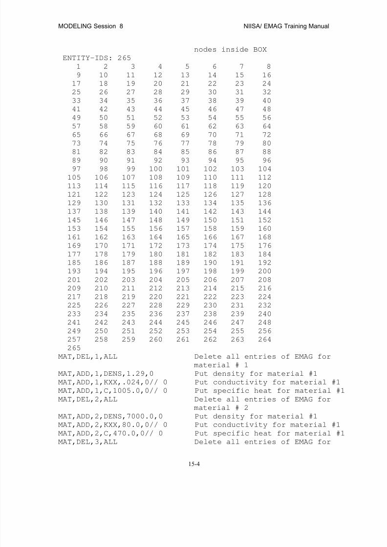
8/12/2019 emagtm
http://slidepdf.com/reader/full/emagtm 230/246
MODELING Session 8 NIISA/ EMAG Training Manual
15-4
nodes inside BOX
ENTITY-IDS: 265
1 2 3 4 5 6 7 8
9 10 11 12 13 14 15 16
17 18 19 20 21 22 23 24
25 26 27 28 29 30 31 32
33 34 35 36 37 38 39 40
41 42 43 44 45 46 47 48
49 50 51 52 53 54 55 56
57 58 59 60 61 62 63 64
65 66 67 68 69 70 71 72
73 74 75 76 77 78 79 80
81 82 83 84 85 86 87 88
89 90 91 92 93 94 95 96
97 98 99 100 101 102 103 104
105 106 107 108 109 110 111 112
113 114 115 116 117 118 119 120
121 122 123 124 125 126 127 128
129 130 131 132 133 134 135 136
137 138 139 140 141 142 143 144
145 146 147 148 149 150 151 152
153 154 155 156 157 158 159 160
161 162 163 164 165 166 167 168
169 170 171 172 173 174 175 176
177 178 179 180 181 182 183 184
185 186 187 188 189 190 191 192
193 194 195 196 197 198 199 200
201 202 203 204 205 206 207 208
209 210 211 212 213 214 215 216217 218 219 220 221 222 223 224
225 226 227 228 229 230 231 232
233 234 235 236 237 238 239 240
241 242 243 244 245 246 247 248
249 250 251 252 253 254 255 256
257 258 259 260 261 262 263 264
265
MAT,DEL,1,ALL Delete all entries of EMAG for
material # 1
MAT,ADD,1,DENS,1.29,0 Put density for material #1
MAT,ADD,1,KXX,.024,0// 0 Put conductivity for material #1MAT,ADD,1,C,1005.0,0// 0 Put specific heat for material #1
MAT,DEL,2,ALL Delete all entries of EMAG for
material # 2
MAT,ADD,2,DENS,7000.0,0 Put density for material #1
MAT,ADD,2,KXX,80.0,0// 0 Put conductivity for material #1
MAT,ADD,2,C,470.0,0// 0 Put specific heat for material #1
MAT,DEL,3,ALL Delete all entries of EMAG for

8/12/2019 emagtm
http://slidepdf.com/reader/full/emagtm 231/246
NISA/ EMAG Training Manual MODELING Session 8
15-5
material # 3
MAT,ADD,3,DENS,8900.0,0 Put density for material #1
MAT,ADD,3,KXX,398.0,0// 0 Put conductivity for material #1
MAT,ADD,3,C,4600.0,0// 0 Put specific heat for material #1
NFORM Select NISA DATA GROUP → NISA
FORMS. Then do the following1. Select TRANSIENT HEAT
a. Select HEATCNTL, put number of iterations = 10 and
save it
b. Select TITLE, put the title and save it
c. Select TEMPERATURE HISTORY, put nodes as 3 and enter
455, 615 and 477
d. Select TEMPERATURE POUT, put time steps as 1 and
enter 0.0 as starting time, 250.0 as ending time and
25.0 as time step.
e. Select TIME INTEGRATION, put time step as 25.0 and
maximum time as 250.0
2. Select EXECUTIVE → THEAT ,enter save file as 26 and 39
and enter filename as DC4H
WRI,NIS,dc4h.nis Write NISA file
Now to do coupled heat analysis you have to do some changes in the NISA files for
EMAG and HEAT . Read these files in an ASCII editor and do changes as follows :
1. For NISA file DC4E.NISa. Enter CHEAT = ON after the line SUBA = SCFL
b. Put SAVE = 26,202. For NISA file DC4H.NIS
a. Enter READ DC4E20.DAT after the *SPTEMP cards
The NISA file DC4E.NIS will look as follows :
**EXECUTIVE data deck for EMAG [EMRC NISA]
ANALYSIS = EFIELD
SUBA = SCFL
FILE = dc4e
SAVE=26,20
CHEAT = ON*TITLE
THERMAL ANALYSIS OF STEEL PLATE (EMAG FILE)
*ELTYPE
1, 104, 1
*NODES
1,,,,-6.00000E-02,-2.00000E-02,-4.00000E-03, 0
2,,,,-6.00000E-02,-2.66667E-02,-4.00000E-03, 0

8/12/2019 emagtm
http://slidepdf.com/reader/full/emagtm 232/246
MODELING Session 8 NIISA/ EMAG Training Manual
15-6
3,,,,-5.66667E-02,-2.66667E-02,-4.00000E-03, 0
4,,,,-5.66667E-02,-2.00000E-02,-4.00000E-03, 0
5,,,,-6.00000E-02,-2.00000E-02,-2.00000E-03, 0
••••••
•••••• ••••••
*ELEMENTS
1, 3, 1, 1, 0
1, 2, 3, 4, 5, 6, 7, 8,
2, 3, 1, 1, 0
2, 9, 10, 3, 6, 11, 12, 7,
3, 3, 1, 1, 0
9, 13, 14, 10, 11, 15, 16, 12,
4, 3, 1, 1, 0
4, 3, 17, 18, 8, 7, 19, 20,
5, 3, 1, 1, 0
3, 10, 21, 17, 7, 12, 22, 19,
••••••
••••••
••••••
*MATEMAG
**STEEL
SIXX, 1,0, 0,0.1E+07,0
**AIR
SIXX, 2,0, 0,0.1E-14,0
**COPPER
SIXX, 3,0, 0,0.58E+08,0
*EMAGCNTL, ID= 1
1,1,1,0.001,1.0
*SPFPOT
** SPFPOT SET = 1
1, 0.00000E+00
2, 0.00000E+00
5, 0.00000E+00
6, 0.00000E+00
9, 0.00000E+00
11, 0.00000E+00
13, 0.00000E+00
15, 0.00000E+00
••••••
••••••

8/12/2019 emagtm
http://slidepdf.com/reader/full/emagtm 233/246
NISA/ EMAG Training Manual MODELING Session 8
15-7
••••••
*ENDDATA
The NISA file DC4H.NIS will look as follows :
ANALYSIS = THEAT
FILE = dc4h
SAVE=26
*TITLE
THERMAL ANALYSIS OF STEEL PLATE (HEAT FILE)
*ELTYPE
1, 104, 1
*NODES
1,,,,-6.00000E-02,-2.00000E-02,-4.00000E-03, 0
2,,,,-6.00000E-02,-2.66667E-02,-4.00000E-03, 0
3,,,,-5.66667E-02,-2.66667E-02,-4.00000E-03, 0
4,,,,-5.66667E-02,-2.00000E-02,-4.00000E-03, 0
5,,,,-6.00000E-02,-2.00000E-02,-2.00000E-03, 0
6,,,,-6.00000E-02,-2.66667E-02,-2.00000E-03, 0
7,,,,-5.66667E-02,-2.66667E-02,-2.00000E-03, 0
8,,,,-5.66667E-02,-2.00000E-02,-2.00000E-03, 0
9,,,,-6.00000E-02,-3.33333E-02,-4.00000E-03, 0
10,,,,-5.66667E-02,-3.33333E-02,-4.00000E-03, 0
••••••
••••••
••••••
*ELEMENTS
1, 3, 1, 1, 0
1, 2, 3, 4, 5, 6, 7, 8,
2, 3, 1, 1, 0
2, 9, 10, 3, 6, 11, 12, 7,
3, 3, 1, 1, 0
9, 13, 14, 10, 11, 15, 16, 12,
4, 3, 1, 1, 0
4, 3, 17, 18, 8, 7, 19, 20,
5, 3, 1, 1, 03, 10, 21, 17, 7, 12, 22, 19,
6, 3, 1, 1, 0
10, 14, 23, 21, 12, 16, 24, 22,
7, 3, 1, 1, 0
18, 17, 25, 26, 20, 19, 27, 28,
8, 3, 1, 1, 0
17, 21, 29, 25, 19, 22, 30, 27,

8/12/2019 emagtm
http://slidepdf.com/reader/full/emagtm 234/246

8/12/2019 emagtm
http://slidepdf.com/reader/full/emagtm 235/246
NISA/ EMAG Training Manual MODELING Session 8
15-9
*TEMPOUT
0.0,250.0,25.0
*ENDDATA
Now you can run the EMAG solver. For DOS version execute NISA386 and choose ELECTRO-MAG (N); for WINDOWS version run EMAGS; for WORKSTATIONS execute EMAG. AT prompt for the input file name type: DC4E.NIS and accept the default DC4E.OUT as the outputfile name. Then you will be asked for the HEAT filename: type DC4H.NIS and DC4H.OUT.
POST-PROCESSING :
DISPLAY III can now be used to view the results of the analysis graphically. Files namedDC4E26.DAT and DC4H26.DAT are created by the EMAG solver when you run it (rememberyou had given these post filenames). These files are needed for post-processing.
Invoke DISPLAY III on your computer. The EMRC logo appears on the screen and the programis ready for interactive usage. By default, the menu mode becomes active so that the user can usethe cursor to execute different commands interactively.
To use this manual effectively, we suggest that you get into the command mode and execute thecommands discussed here by typing in from keyboard. After getting comfortable with this procedure, you should experiment with the menu mode and follow similar steps for post- processing results.
To get into the command mode, you need to move the cursor into the area on the screendisplaying ‘COMMAND’ and hit the ENTER key. You may also type in the letter ‘C’ to get intothe command mode.
For this session only one plot is viewed. You are encouraged to make use of the on-line HELPoption and experiment with various other options available to generate other plots of interest.
You have already seen the post processing results for DC4E26.DAT. For post-processing ofHEAT analysis, type the following commands
COMMANDS DESCRIPTION
REA,POS,dc4h26.dat Read the post processing data
file
CTR,ADD,TEMP Select contour as temperature
CTR,CLB,LNUM Select contour plotting as lines
with numbers
PLO Regenerate the plot
VEW,ANG1 View plot at viewing angle 1

8/12/2019 emagtm
http://slidepdf.com/reader/full/emagtm 236/246
MODELING Session 8 NIISA/ EMAG Training Manual
15-10
VEW,BND,ON Put boundary line plotting for all
elements on
PLO Regenerate the plot
Figure 15.1 The temperature distribution
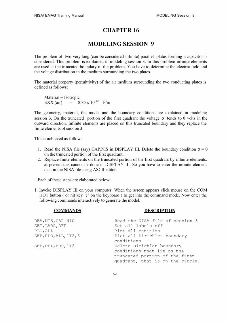
8/12/2019 emagtm
http://slidepdf.com/reader/full/emagtm 237/246
NISA/ EMAG Training Manual MODELING Session 9
16-1
CHAPTER 16
MODELING SESSION 9
The problem of two very long (can be considered infinite) parallel plates forming a capacitor isconsidered. This problem is explained in modeling session 3. In this problem infinite elementsare used at the truncated boundary of the problem. You have to determine the electric field andthe voltage distribution in the medium surrounding the two plates.
The material property (permittivity) of the air medium surrounding the two conducting plates isdefined as follows:
Material = IsotropicEXX (air) = 8.85 x 10⁻¹² F/m
The geometry, material, the model and the boundary conditions are explained in modelingsession 3. On the truncated portion of the first quadrant the voltage φ tends to 0 volts in theoutward direction. Infinite elements are placed on this truncated boundary and they replace thefinite elements of session 3.
This is achieved as follows
1. Read the NISA file (say) CAP.NIS in DISPLAY III. Delete the boundary condition φ = 0on the truncated portion of the first quadrant.
2. Replace finite elements on the truncated portion of the first quadrant by infinite elements:at present this cannot be done in DISPLAY III. So you have to enter the infinite element
data in the NISA file using ASCII editor.
Each of these steps are elaborated below:
1. Invoke DISPLAY III on your computer. When the screen appears click mouse on the COMHOT button ( or hit key ‘c’ on the keyboard ) to get into the command mode. Now enter thefollowing commands interactively to generate the model.
COMMANDS DESCRIPTION
REA,NIS,CAP.NIS Read the NISA file of session 3
SET,LABA,OFF Set all labels offPLO,ALL Plot all entities
SFP,PLO,ALL,1T2,8 Plot all Dirichlet boundary
conditions
SFP,DEL,BRD,1T2 Delete Dirichlet boundary
conditions that lie on the
truncated portion of the first
quadrant, that is on the circle.

8/12/2019 emagtm
http://slidepdf.com/reader/full/emagtm 238/246
MODELING Session 9 NIISA/ EMAG Training Manual
16-2
ENTITY-IDS: 17
82 83 84 85 86 87 88 89
90 190 191 192 193 194 195 196
197
PLO Regenerate the plot
ELE,FAC,162 Find the faces of elements that
ELE,FAC,165 lie on the truncated portion of
ELE,FAC,65 the first quadrant. Find the face
ELE,FAC,68 that tends to infinity. You will
Find that this face is # 1 for all
elements on truncated portion.
PLO Regenerate the plot
ELE,SRH,BRD Now search all elements that lie
on the truncated portion boundary.
Note these numbers for future use
ENTITY-IDS: 16
65 66 67 68 69 70 71 72
161 162 163 164 165 166 167 168
WRI NIS CAP9.NIS Write the modified NISA file
END Quit DISPLAY III
2.Invoke an ASCII editor. Read file CAP9.NIS, which is an ASCII
file. Now before you commence changes in the file, please note
the format for including infinite elements in your model. At
present you cannot prescribe these elements in DISPLAY III :
so you have to describe them in NISA file according to a
format as shown below :
******************************************************************************
*INFELE data group - Element specified as infinite element and direction of infinity
Applicable analysis types: EFIELD, MFIELD
This data group may be used in all types of analysis: electric field or magnetic field tospecify which elements are infinite, the infinite element type, which faces of the infiniteelement go to infinity and the choice of number of Gaussian points. The data group isvalid for 2D and 3D.
Group ID card: *INFELE
Free format data for a typical infinite element input consists of two card sets
Card set 1 : Element identification card (one card)
Entry No : 1 2 3
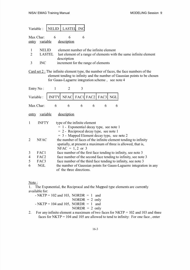
8/12/2019 emagtm
http://slidepdf.com/reader/full/emagtm 239/246
NISA/ EMAG Training Manual MODELING Session 9
16-3
Variable : NELID LASTEL INC
Max Char: 6 6 6entry variable description
1 NELID element number of the infinite element2 LASTEL last element of a range of elements with the same infinite element
description3 INC increment for the range of elements
Card set 2 : The infinite element type, the number of faces, the face numbers of theelement tending to infinity and the number of Gaussian points to be chosenfor Gauss-Laguerre integration scheme , see note 4
Entry No : 1 2 3
Variable : INFTY NFAC FAC1 FAC2 FAC3 NGL
Max Char: 6 6 6 6 6 6
entry variable description
1 INFTY type of the infinite element= 1 - Exponential decay type, see note 1= 2 - Reciprocal decay type, see note 1= 3 - Mapped Element decay type, see note 2
2 NFAC the number of faces of the infinite element tending to infinityspatially, at present a maximum of three is allowed, that is, NFAC = 1, 2 or 3
3 FAC1 face number of the first face tending to infinity, see note 34 FAC2 face number of the second face tending to infinity, see note 35 FAC3 face number of the third face tending to infinity, see note 36 NGL the number of Gaussian points for Gauss-Laguerre integration in any
of the three directions.
Note :1. The Exponential, the Reciprocal and the Mapped type elements are currentlyavailable for:
- NKTP = 102 and 103, NORDR = 1 and NORDR = 2 only
- NKTP = 104 and 105, NORDR = 1 and NORDR = 2 only
2. For any infinite element a maximum of two faces for NKTP = 102 and 103 and threefaces for NKTP = 104 and 105 are allowed to tend to infinity: For one face , enter

8/12/2019 emagtm
http://slidepdf.com/reader/full/emagtm 240/246
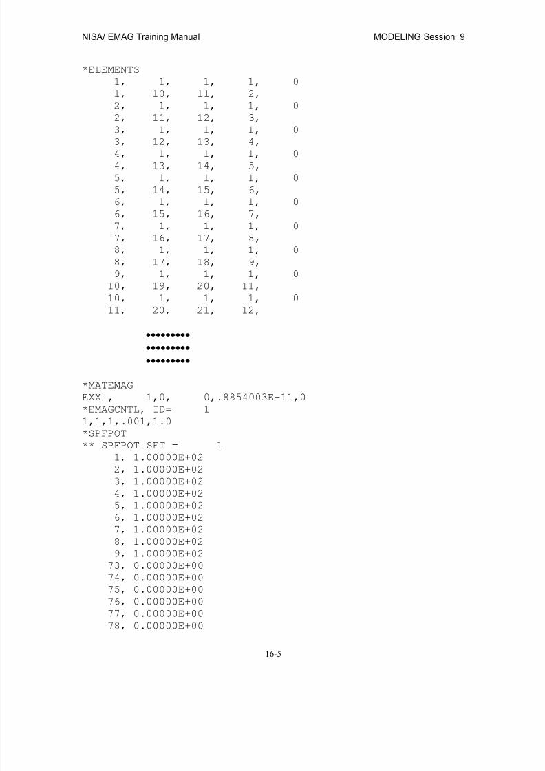
8/12/2019 emagtm
http://slidepdf.com/reader/full/emagtm 241/246
NISA/ EMAG Training Manual MODELING Session 9
16-5
*ELEMENTS
1, 1, 1, 1, 0
1, 10, 11, 2,
2, 1, 1, 1, 0
2, 11, 12, 3,
3, 1, 1, 1, 0
3, 12, 13, 4,
4, 1, 1, 1, 0
4, 13, 14, 5,
5, 1, 1, 1, 0
5, 14, 15, 6,
6, 1, 1, 1, 0
6, 15, 16, 7,
7, 1, 1, 1, 0
7, 16, 17, 8,
8, 1, 1, 1, 0
8, 17, 18, 9,
9, 1, 1, 1, 0
10, 19, 20, 11,
10, 1, 1, 1, 0
11, 20, 21, 12,
•••••••••
•••••••••
•••••••••
*MATEMAG
EXX , 1,0, 0,.8854003E-11,0
*EMAGCNTL, ID= 1
1,1,1,.001,1.0
*SPFPOT
** SPFPOT SET = 1
1, 1.00000E+02
2, 1.00000E+02
3, 1.00000E+02
4, 1.00000E+02
5, 1.00000E+02
6, 1.00000E+02
7, 1.00000E+02
8, 1.00000E+029, 1.00000E+02
73, 0.00000E+00
74, 0.00000E+00
75, 0.00000E+00
76, 0.00000E+00
77, 0.00000E+00
78, 0.00000E+00

8/12/2019 emagtm
http://slidepdf.com/reader/full/emagtm 242/246
MODELING Session 9 NIISA/ EMAG Training Manual
16-6
79, 0.00000E+00
80, 0.00000E+00
81, 0.00000E+00
190, 0.00000E+00
198, 0.00000E+00
206, 0.00000E+00
214, 0.00000E+00
222, 0.00000E+00
230, 0.00000E+00
238, 0.00000E+00
246, 0.00000E+00
254, 0.00000E+00
262, 0.00000E+00
270, 0.00000E+00
278, 0.00000E+00
*INFELE
65,,,
3,1,1,0,0,2
66,,,
3,1,1,0,0,2
67,,,
3,1,1,0,0,2
68,,,
3,1,1,0,0,2
69,,,
3,1,1,0,0,2
70,,,
3,1,1,0,0,2
71,,,3,1,1,0,0,2
72,,,
3,1,1,0,0,2
161,,,
3,1,1,0,0,2
162,,,
3,1,1,0,0,2
163,,,
3,1,1,0,0,2
164,,,
3,1,1,0,0,2165,,,
3,1,1,0,0,2
166,,,
3,1,1,0,0,2
167,,,
3,1,1,0,0,2
168,,,

8/12/2019 emagtm
http://slidepdf.com/reader/full/emagtm 243/246
NISA/ EMAG Training Manual MODELING Session 9
16-7
3,1,1,0,0,2
*ENDDATA
Save the file CAP9.NIS.
Now you can run the EMAG solver. For DOS version execute NISA386 and choose ELECTRO-MAG (N); for WINDOWS version run EMAGS; for WORKSTATIONS execute EMAG. AT prompt for the input file name type: CAP9.NIS and accept the default CAP9.OUT as the outputfile name.
POST-PROCESSING :
DISPLAY III can now be used to view the results of the analysis graphically. A file namedCAP926.DAT is created by the EMAG solver when you run it (remember you had given the postfilename as CAP9). This file is needed for post-processing.
Invoke DISPLAY III on your computer. The EMRC logo appears on the screen and the programis ready for interactive usage. By default, the menu mode becomes active so that the user can usethe cursor to execute different commands interactively.
To use this manual effectively, we suggest that you get into the command mode and execute thecommands discussed here by typing in from keyboard. After getting comfortable with this procedure, you should experiment with the menu mode and follow similar steps for post- processing results.
To get into the command mode, you need to move the cursor into the area on the screendisplaying ‘COMMAND’ and hit the ENTER key. You may also type in the letter ‘C’ to get intothe command mode.
For this session only one plot is viewed. You are encouraged to make use of the on-line HELPoption and experiment with various other options available to generate other plots of interest.
For post-processing, type the following commands
COMMANDS DESCRIPTION
REA,POS,cap926.dat Read the post processing data
file
CTR,ADD,VOLT Select contour as Voltage
CTR,CLB,LNUM Select contour plotting as lines
with numbers
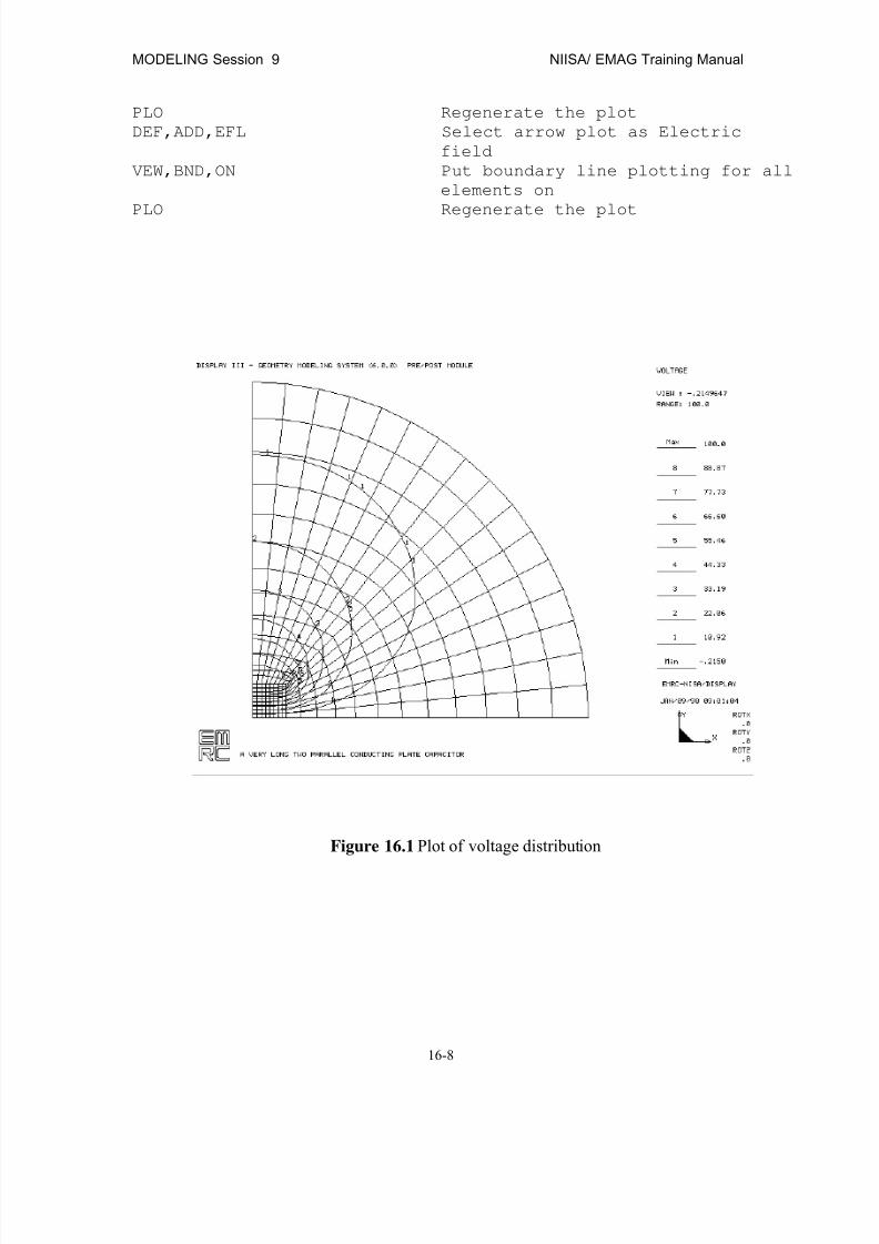
8/12/2019 emagtm
http://slidepdf.com/reader/full/emagtm 244/246
MODELING Session 9 NIISA/ EMAG Training Manual
16-8
PLO Regenerate the plot
DEF,ADD,EFL Select arrow plot as Electric
field
VEW,BND,ON Put boundary line plotting for all
elements on
PLO Regenerate the plot
Figure 16.1 Plot of voltage distribution

8/12/2019 emagtm
http://slidepdf.com/reader/full/emagtm 245/246
NISA/ EMAG Training Manual MODELING Session 9
16-9
Figure 16.2 Arrow field plot of electric field distribution

8/12/2019 emagtm
http://slidepdf.com/reader/full/emagtm 246/246
MODELING Session 9 NIISA/ EMAG Training Manual


