Elements of Control

2.830 Control of Manufacturing Processes April 9, 2000

1

Massachusetts Institute of Technology Department of Mechanical Engineering

2.830 Control of Manufacturing Processes

Elements of Control

by D. Hardt

Introduction Proper analysis of the myriad manufacturing processes requires a bewildering breadth of physical understanding, easily beyond the reach of any one specialist. However, the control approach taken here is intended to overcome this vastness by referring all processes to a common body of theory, that of feedback control systems. While this theory itself has many different aspects and many limitations, our objective is to develop a common perspective for viewing processes and their control based on linear system theory and classic control concepts. No direct background in control theory is assumed, only a familiarity with ordinary differential equations. Throughout this note, we concentrate on a single example system: the DC motor servo control problem. This is not only a convenient system to model and analyze, it also is the basic building block for many manufacturing control systems. As a result, the material is important even for those with a solid grounding in linear control theory.

Causality/control model The basic "control perspective" is one of an input-output system with clear causality. Regardless of the details of the particular process we plan to control, we can — and indeed must — describe the process in a causal or input-output fashion. Few, if any, manufacturing processes can be considered simple linear systems, but in some cases the restrictions can be violated without negating the utility of control theory. However, while the power of the control approach is to provide a well defined model form, learning the inherent limitations of this form will be an important element in the course. A manufacturing process is a system that modulates the energy interaction between machine and material such that geometry and property transformations of the material take place. The process begins with design specifications based on which the energy modulation is prescribed to produce the desired material transformation. One way to prescribe the energy modulation is a trial-and-error approach in which many runs are made, each with different settings from another’s, such that at least one setting will result in the desired outputs; however, the cost and waste associated with this approach are very high. Another way is to predict the required energy input to produce the desired outputs; however, the approach requires a very accurate model of the process describing its behavior precisely. If such a model were available, we can always “invert” our plant to obtain the required energy input based on the prescribed outputs. This ideal approach is represented in Fig A bellow.

Figure A Energy Modulation to Obtain Desired Output.


2

It is unfortunate that modeling a manufacturing process precisely is very difficult if not impossible. Moreover, the calculated input will not be able to compensate for unknown disturbances to the plant. Therefore, it is essential to modulate the input into the plant according to the difference between the prescribed and actual outputs as shown in Fig B below.

Figure B Basic Structure of Feedback System.

A mathematical representation of the above structure is given as

Y =CP

1 + C PR +

11+ C P

D (A)

in which the objectives are to have Y = R as well as to reject the effect of disturbance D on the output Y. We can now vary the control gain C to achieve the tracking and disturbance rejection objectives of a feedback control system. It is obvious that as the combined gain of controller and plant CP is much larger than 1 then Y will assume a value very close to R and the effect of disturbance D on the output will be minimal.

The Feedback Control system: Structure and Properties The basic layout of a feedback or closed-loop control system is shown in Fig 1. The essential elements of this system are shown in the figure, and include the plant (the system to be controlled), the measurement (sensors, estimators and signal conditioners), the controller (the system we create to implement a control law or algorithm) and the error junction (where the desired system outputs and the measured or estimated outputs are compared to generate the error). Als o evident from this diagram are the various signals in the system. (Careful adherence to the definition of these signals is important; it will prevent confusion in later discussions when manipulating process control system gets more complex and less similar in form to Fig 1).

Controller

Measurement

Actuator Plantr e u

d

y

-

+ ++

Figure 1 A Canonical Feedback Control System The system output y is the physical quantity we wish to regulate. The input to the control system is actually the desired output or setpoint r. When measured outputs and setpoint are compared, we generate the error e, which is the signal upon which all of our control actions are based. The controller then takes this error and creates a control output u, which serves as an input (through an actuator) to the plant. Finally, there is the disturbance d, which we will define as any influence that causes undesired changes in the output. (This disturbance can enter the system in many places, not just that shown in Fig 1)


3

Study Problem: The Position Servo To review the basics of classic control theory, we will deal with a single example system: the position servomechanism. Most manufacturing equipment, if it entails any level of automation, comprises, at least, a position servo. Combined with a digital computer, the position servo imb ues any machine with programmable motion of great precision. The problems in servo analysis and design are quite similar to those encountered in other “parameter” or machine control problems (such as force, pressure, flow, or temperature control) and is a system that is well modeled by standard linear system methods. However, linearity makes the specifics of servo controller design quite different from those of a typical manufacturing process. Accordingly, it is important to realize the idealized nature of the ensuing development, and that it is providing the basic underpinnings, but not the direct analog for manufacturing process control. A simple position servo is shown in Fig 2, and below it is a block diagram, showing how each element is connected. Notice that the system involves feedback, and that the key elements in a feedback system: measurement, comparison, error generation and actuation, are all included. In operation, the error signal is generated by a difference between the desired position and the actual position. This error is sent to the controller, where it may be amplified or filtered to create the actuator signal u. The actuator signal is sent to a power amplifier, where the signal is converted to a level of power sufficient to drive the motor. The motor torque causes the load to move, and this motion leads to a position change, which (if the system is correctly constructed) will reduce the error to zero. Thus the system automatically causes the input and output to match.

Controller

Reference (θr)

Amplifier DC Motor

LoadMeasurementTransducer (θ)u I

Power

Controller Amplifier Motor/Loade u

-

+ Iθr θ

Fig 2 A Simple Position Servo and Equivalent Block Diagram To begin the analysis of this system, it is first necessary to describe both the static and dynamic behavior of the basic elements, in this case the amplifier, motor and measurement transducer. To do this, we must first develop a basic system dynamics methodology.

Linear Dynamic Processes Classic control theory is based upon the concept of linear stationary dynamic systems. Such systems are those that are adequately described by ordinary, linear, time-differential equations, with constant (i.e. stationary) coefficients. As an example, consider a simple spring mass system, shown in Fig 3. For this system, the


4

governing equation is derived from a force balance, with appropriate constitutive relations for stiffness and damping:

ΣF = m x = Fspring + Fdamper + Fext

Fspring = -k x

Fdamper = -b x

mx + bx + kx = Fext (1)

Fext

k

m

b

Figure 3 Simple Spring Mass Dynamic Systems

As Eqn 1 implies, the resulting differential equation is ordinary (no partial derivatives), and linear ( all variables and their derivatives are mu ltiplied only by constants). For this physical system we can also illustrate the linearity by looking at the basic constitutive equations for the spring and damper (see Eqn 1). Notice that for each one, the force is a linear function of the “input” (either displacement or velocity). These linear elements combine in a linear equation based on Newton’s laws to yield a linear system. Linear differential equations are attractive because they have simple, well behaved solutions, and these solutions have the property of superposition. This latter point is most important to control system analysis, where many and varied types of inputs are often present. With superposition these inputs can be decomposed into sets of standard inputs, for which well known solutions (i.e. outputs) are known. These outputs can then be summed to yield the total system response. The true virtue of linear systems, therefore, is that we can analyze complex systems by artful combinations of various simple systems, and predict the effect of changing these inputs or even the system itself based on this knowledge.

Step 1: Modeling the Plant The first step is to create a model of the DC motor and load in the servo system of Fig While the motor is a rather complex electromechanical device, the basic constitutive relationship (for a motor with a permanent magnet field and a commutated armature) can be approximated by: Tm = Kt I (2) where Tm is the motor torque, I is the current in the motor, and Kt is the motor “torque constant”. The torque constant is determined by motor characteristics such as radius, length, number of windings, and field magnet strength. If the motor is operated in a current driven mode (i.e. the amplifier in Fig 2 provides a current output in proportion to the actuation input u), then it is clear that the motor is a linear device. What if our concern is not with the torque output of the motor, but with the resulting shaft speed ΩΩ ? To determine ΩΩ , we must consider the load on the motor, in this case a simple rotational inertia J, and a bearing viscous damping b. From this we obtain the dynamics of the mechanical part of the motor system:

Σ T = JΩ = Tm - bΩ (3) Combining Eqn 2 and 3 gives the model for the motor with current I as the input and speed ΩΩ as the output:


5

JΩ + bΩ = K t I

or

J/b Ω + Ω = K t/b I (4) This is a simple first order linear differential equation.1 The solution of this equation is well know for several basic inputs. The most common of these is the “step” input, where the current is changed instantaneously from one value to another. The solution to Eqn 4 when I is changed in a stepwise fashion is given by:

Ω ( t) = Ω ss 1 − exp − bJ t( )[ ] (5)

This response is shown in Fig 4, and it can be seen that acceleration (slope) continuously decreases until the steady state velocity, given by the following expression, is reached:

Ωss = Kt

b I

(6) Figure 4 also illustrates the concept of a time constant or characteristic response time. For the exponential response it is defined as the time, τ , at which the argument of the exponential is unity. Thus, from Eqn 5, we can define the time constant of the motor as:

τm = Jb

and Eqn 5 can be rewritten for a general output y: y(t) = yss (1 - e-t/τ) (7) Equation 7 is in fact the general expression for any first order differential equation subjected to a step input, and any physical system that is described by a linear first order differential equation will have this step response. However, this simple solution alone is insufficient for designing a control system, since we need a means of concatenating the elements in the control block diagram, and of analyzing the resulting linear system.

1Notice that we cannot separate the motor and load because they are coupled dynamically as indicated in this expression. This is a very simple case of preserving input - output causality which will become an important issue in separating machine and process in later chapters.


6

τ

0

0.5

1

0 2 4 6 8 10 12Time

Ω/Ωss

0.63

Fig 4 Step Response for a First Order System with a Time Constant = 2.0 sec.

Governing equations

The block diagram in Fig 1 was constructed both to show the interconnection of each of the elements of the system, and to show the transformation occurring within each block. The contents of each block can be thought of as an operator that transforms the input into a corresponding output. For the motor/load block, this transformation is given by Eqn 4. However, we need to use a more tractable form than the time differential equation. For this we will transform the differential equations to algebraic equations using operator notation. The actual mathematics of this transformation are governed by the Laplace Transform2. However, for this treatment, we will consider only the use of algebraic operators to illustrate this transformation. For the sake of brevity, it will just be given that the following derivative and integral expressions in t can be replaced by the corresponding algebraic expressions in s.

ddt

f (t ) ⇒ sF(s ) − f (0 )

d2

dt2 f (t) ⇒ s2F (s) − sf (0) − Ý f (0 )

2 The Laplace Transform of a time function y(t) is a continuous transform given by the expression:

Ly(t) = y(t) e-stdt

0+

∞

= Y(s)

This transform can be used to solve complex differential equation and a variant of this, the Fourier Transform, is quite useful in the “frequency analysis” of linear system. Further information on the Laplace Transform in the context of classical control analysis can be found in: Ogata, Modern Control Principles, Wiley, 1983 Dorf, Modern Control Systems, Prentice Hall, 1982.


7

f (t)dt

0

t

∫ ⇒1s

F (s ) (8)

Any linear, constant coefficient time-differential equation can be transformed into an algebraic equation in s. Since we can analyze control systems from a “zero” initial state, the initial conditions and integration constants

in Eqn 8 vanish, and the most important result is that ddt

f (t)( )⇒ sF(s ).

Applying these operators to the motor equation in 3 yields: J Ý Ω (t ) + bΩ (t) = Kt I(t) ⇒ JsΩ (s) + bΩ (s) = Kt I (s) ( Js + b)Ω (s ) = Kt I (s ) (9) Notice that the variables Ω and I are shown as functions of s rather than time t, since the transformation has been applied. It is the second expression in Eqn 9 that is so powerful, since with a simple manipulation, we can derive a transfer function that is in fact the input/output relationship for the motor block:

Ω (s)

I(s)=

K tJs + b

= G p( s) (10)

Defining the right hand expression in Eqn 10 as the transfer function Gp(s) , the motor/load block in Fig 2 can be represented in a simple form:

Gp(s)Ω (s)I (s)

Ω (s) = G p(s) I (s)

Now we have a compact and algebraically simple means of describing the content of each of the blocks. The content of each block is the transfer function for the process involved, and the output of each block is found simply by multiplying the input by the transfer function. Once the transfer function is defined, it can be analyzed to determine the static and dynamic characteristics of the block. The transfer function for the motor, which is the same as for any first order system, can be written in a generic form by using the time constant and steady state gain definitions given above. Thus, a general transfer function for a first order system is:

G(s) =K

τs + 1 (12)

For the motor example, K = Kt/b and τ = J/b. The denominator of the transfer function (τs + 1, in this case) corresponds to the left-hand side of the original time differential equation. When the denominator is set equal to zero, it is called the characteristic equation, the roots of which correspond to the inverse of the characteristic response times of the system. For our simple first order system in Eqn 12, the characteristic equation is: τs + 1 = 0 (13) and the root of this equation is -1/τ. It should be apparent from Fig 4 that this one root is sufficient to completely determine the shape of the response curve, while the actual magnitude is determined by the size of the input and the steady state gain K.


8

Leaving the motor example for a moment, it is evident that higher order differential equations will be encountered in more complex systems. The resulting transfer functions will simply have higher order characteristic equations. As will be shown below, however, linear systems of any order can be decomposed into products of simple first and second order terms. This result follows directly from the observation that any polynomial has (at most) only real and/or complex conjugate roots: the real roots corresponding to first order terms and each complex conjugate pair corresponding to a single second order term.

Control Example: Velocity Servo Before attacking the complete position servo of Fig 2, consider controlling the speed of the DC motor. Inspection of the motor transfer function makes this look like a trivial problem, since we need only provide the current I that will provide the desired speed. This so-called open-loop control can be applied when the transfer function is completely and perfectly known, but this is seldom the case for any real system. In the case of the motor, “reality” will be in the form of unexpected loads imposed by the environment into which the motor/load system is placed and uncertainty as to the motor constant Kt, the bearing damping b, and the load inertia magnitude J. In this analysis, the unexpected load is modeled as a disturbance torque that may arise from friction or other forms of external resistance to motion. It could just as well represent additional sources of power that are undesirable (such as a wind force on a rotating tower, or, if this were a vehicle, the gravitational force from moving downhill). The updated motor model now has the following form, with the torque disturbance represented by Td and time derivatives eliminated by using the operators in Eqn 8. Σ T = J Ý Ω = Tm − bΩ + Td J Ý Ω + bΩ = Kt I + Td

Ω ( s) =Kt

Js + bI (s ) +

1Js + b

Td (s )

=

Kt

bJ

bs + 1

I (s) +

1b

J

bs + 1

Td ( s)

= Gp (s ) ⋅ I(s ) +1Kt

Gp (s) ⋅ Td ( s)

(13)

The block diagram for the motor must now be updated to show this new input:

Gp(s)

1/Kt

I (s) Ω (s)

Td

++


9

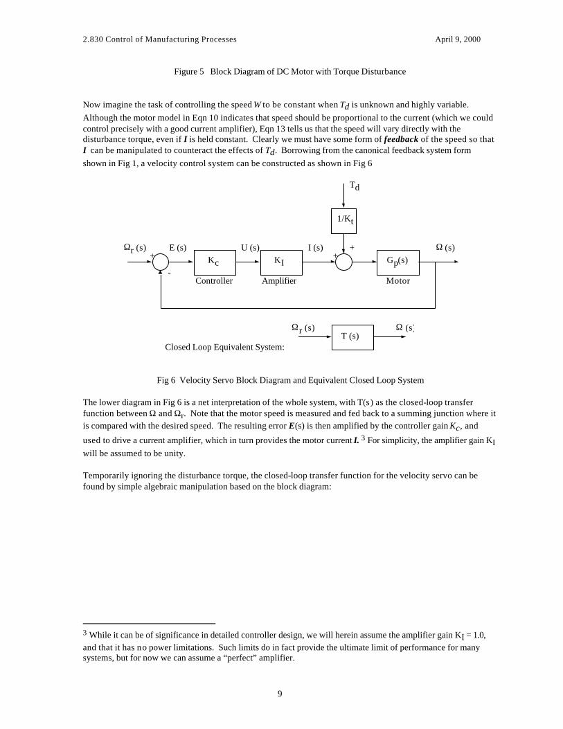
Figure 5 Block Diagram of DC Motor with Torque Disturbance Now imagine the task of controlling the speed Ω to be constant when Td is unknown and highly variable. Although the motor model in Eqn 10 indicates that speed should be proportional to the current (which we could control precisely with a good current amplifier), Eqn 13 tells us that the speed will vary directly with the disturbance torque, even if I is held constant. Clearly we must have some form of feedback of the speed so that I can be manipulated to counteract the effects of Td. Borrowing from the canonical feedback system form shown in Fig 1, a velocity control system can be constructed as shown in Fig 6

Gp(s)

1/Kt

I (s)

Td

++

U (s)E (s)Ωr (s)+ Kc KI

-Controller Amplifier Motor

Ω (s)

Closed Loop Equivalent System: T (s)

Ωr (s) Ω (s)

Fig 6 Velocity Servo Block Diagram and Equivalent Closed Loop System The lower diagram in Fig 6 is a net interpretation of the whole system, with T(s) as the closed-loop transfer function between Ω and Ωr. Note that the motor speed is measured and fed back to a summing junction where it is compared with the desired speed. The resulting error E(s) is then amplified by the controller gain Kc, and

used to drive a current amplifier, which in turn provides the motor current I. 3 For simplicity, the amplifier gain KI will be assumed to be unity. Temporarily ignoring the disturbance torque, the closed-loop transfer function for the velocity servo can be found by simple algebraic manipulation based on the block diagram:

3 While it can be of significance in detailed controller design, we will herein assume the amplifier gain KI = 1.0, and that it has no power limitations. Such limits do in fact provide the ultimate limit of performance for many systems, but for now we can assume a “perfect” amplifier.


10

Ω ( s) = Gp (s )⋅ I(s )

I(s) = Kc Ωr ( s) − Ω (s)( )

Ω ( s) = Gp (s )⋅ Kc Ωr (s ) − Ω ( s)( )

Ω ( s)

Ω r (s)=

G pK c

1+ Gp Kc

(14)

From the last expression, it is clear that the closed-loop transfer function T(s) is defined as:

T(s) ≡

GpKc

1 + GpKc (15) since it relates the overall system output to the reference or command input. Substituting for Gp(s) from Eqn 12 yields (and using substitutions Km = Kt/b and τm = J/b):

G p (s) =Km

τms +1

T (s) =

KcKmτms + 1

1 + Kc Kmτ ms +1

=

Kc Km1 + KcKm

τm1+ Kc Km

s + 1

=KT

τTs + 1 (16)

Equation 16 still represents a first order transfer function, but with new definitions for K and τ. A close look at these new system parameters will reveal the properties of this feedback system. Notice first of all that the steady state gain KT will never be greater than one, and in fact will only reach unity when Kc → ∞. Thus, this system will never achieve exact command following, but can only approach it as the gains are increased. This apparent drawback is immediately counteracted by the observation that the closed-loop steady-state gain, KT, is determined by both Kc (which we can easily adjust) and Km (which is a fixed property of the motor). Thus, if Km varies (which it can over time as the components age, or as the temperature of the motor changes) the effect on the steady-state performance of the control system will be slight, provided Kc is large relative to Km. This illustrates the reduction in sensitivity to parameter changes in the system that is achieved by feedback, and this will come to be a most important property as we investigate manufacturing processes where the process gains will be highly variable, and uncertain. Furthermore, we will see below that it is possible to design a controller that can completely eliminate the effects of parameter changes at steady-state and provide zero error. Now consider the effect of feedback on the dynamics of the new system. The closed loop time constant τT in Eqn 16 demonstrates that as the product KcKm is increased, the time constant of the closed loop system will decrease leading to a shorter time required to settle after an input change. Thus the effect is clear: the addition of feedback can change the apparent time constant of the motor. Theoretically the gain Kc can be made arbitrarily high to achieve any desired time constant, but the ultimate limit on how fast the motor can respond is typically the power capability of the current amplifier or the heat dissipation capacity of the motor. With this


11

simple example we can see that feedback aids in reducing variations in the motor speed and improves the response time of the basic motor.

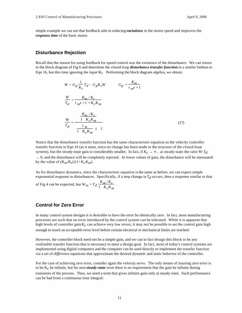
Disturbance Rejection Recall that the reason for using feedback for speed control was the existence of the disturbance. We can return to the block diagram of Fig 6 and determine the closed-loop disturbance transfer function in a similar fashion to Eqn 16, but this time ignoring the input Ωr. Performing the block diagram algebra, we obtain:

Ω = G p1

K tTd − G pKcΩ Gp =

Kmτms + 1

ΩTd

=Km / Kt

τms + 1 + KcKm

ΩTd

=

Km / K t1+ KcKm

τ m1+ KcKm

s + 1

(17)

Notice that the disturbance transfer function has the same characteristic equation as the velocity controller transfer function in Eqn 16 (as it must, since no change has been made to the structure of the closed-loop system), but the steady-state gain is considerably smaller. In fact, if Kc → ∞ , at steady-state the ratio Ω/ Td → 0, and the disturbance will be completely rejected. At lower values of gain, the disturbance will be attenuated by the value of (Km/Kt)/(1+KcKm). As for disturbance dynamics, since the characteristic equation is the same as before, we can expect simple exponential response to disturbances. Specifically, if a step change in Td occurs, then a response similar to that

of Fig 4 can be expected, but Ω ss = TdKm / K t

1+ KcKm .

Control for Zero Error In many control system designs it is desirable to have the error be identically zero. In fact, most manufacturing processes are such that no error introduced by the control system can be tolerated. While it is apparent that high levels of controller gain Kc can achieve very low errors, it may not be possible to set the control gain high enough to reach an acceptable error level before certain electrical or mechanical limits are reached. However, the controller block need not be a simple gain, and we can in fact design this block to be any realizable transfer function that is necessary to meet a design goal. In fact, most of today's control systems are implemented using digital computers and the computer can be used directly to implement the transfer function via a set of difference equations that approximate the desired dynamic and static behavior of the controller. For the case of achieving zero error, consider again the velocity servo. The only means of insuring zero error is to let Kc be infinite, but for zero steady-state error there is no requirement that the gain be infinite during transients of the process. Thus, we need a term that gives infinite gain only at steady state. Such performance can be had from a continuous time integral:


12

⌡⌠o

t

(.) dt = 1s ( ) (18)

The infinite steady-state gain arises since a constant integrand (e.g. the error signal) will cause this integral to approach infinity as t →∞ (which is in fact the definition of “steady state”). This integral controller for the velocity servo is shown in Fig 7

Gp(s)

1/Kt

I (s)

Td

++

Ωr (s)+

-

Ω (s)Kc / s

Figure 7 Velocity Servo with Integral Control

To determine the net effect of this change on the closed-loop system, we again perform block diagram algebra on this system (ignoring Td), substituting Kc/s for Kc in the previous development of Eqn 16:

T(s) ≡ Gp

Kcs

1 + GpKcs

and sustituting for Gp(s):

T(s) =

KcKmτm

s 2 + 1τm

s + KcKmτm (19)

Notice now that the denominator is of second order, since the integral controller adds a time dependent element to the system. To examine the steady state we let all terms in s vanish (which is equivalent to letting all time derivatives vanish. Now the steady state gain of T(s) in Eqn 19 is unity, regardless of the values for Kc, Km or ττ m. Thus Ω(s) = Ωr(s) and the objective of zero steady-state error is achieved. It is important to examine the effect of this controller on the system dynamics. Clearly there has been a change since the characteristic equation is now of the form (b and c are arbitrary constants, no relation to damping b):


13

s 2 + 1τm

s + KcKmτm

= 0

or

s 2 + b s + c = 0 (20) The new dynamics are found by considering the roots of this characteristic equation. Since it is a quadratic, the roots are given by:

s1, s2 = - b

2 ± b 2-4c

2 (21) and these roots will be either real and negative (if the radical is positive) or complex conjugates (if the radical is negative). If the roots are real, the result is basically two first order roots, and the resulting dynamics will simply be the sum of the response of each of these terms and will resemble the plot shown in Fig 8, which shows the step response of a second order system where the two roots are nearly identical.

Figure 8 Step Response of a Integral Velocity Controller with two Real Roots of Similar Magnitude

However, if the value of the parameters is such that the radical in Eqn 21 is negative, the roots will be complex. To better understand the resulting system response, we first make the following substitutions:

s 2 + b s + c = 0 ⇓ ⇓

s 2 + 2ζωn s + ωn2 = 0 (22)

where the equation has been parameterized by the terms ζ ≡ damping ratio and ωn ≡ natural frequency. The solution of this characteristic equation leads to the step response given by:


14

Ω ( t) = Ω SS(1 − Be−ζωn t ) sin(ωd t + φ)

where

B =1

1 − ζ 2 φ = tan−1 1 − ζ 2

ζ

ω d = ωn 1 − ζ 2

(23)

The response will be a sinusoid of frequency ωω d (the damped natural frequency), with a magnitude envelope given by the exponential term B exp(-ζωnt). This response is illustrated in Figure 9 for various values of ζ. It is apparent that the natural frequency determines the time scale of the response while the damping ratio determines the shape of the envelope within which the response occurs. (Notice that the rate of decay (or time constant) of this envelope is given by the product ζ ωn). Most obvious is the fact that as ζ decreases, the degree of overshoot beyond the eventual steady-state value, and the degree of oscillation both increase. When ζ = 1 (critical damping) the response is again that of two simple exponentials, each with equal roots.

Ω/Ω ss

Time

ζ = 0.25

ζ = 0.707ζ = 0.5

ζ = 1.0

Fig 9 Second Order System Response for Complex Roots

Position Control The above example dealt only with the problem of speed control, whereas we eventually want to control the position of a manufacturing machine. Implementation of the position control is quite simple, requiring only that a position measurement be made, as shown in the original servo (Fig 2). The details of this measurement and its actual location in the mechanism are quite important, but for this discussion the ideal case shown in Fig 2 is assumed. For the moment we will also abandon the velocity loop designed above, and concentrate on the position loop only. The block diagram for the position control system, showing the various transfer functions, is shown in Fig 10. The motor block still has Ω as the output, but the position measurement is represented with an integrator block. Thus the measurement of position from a velocity output device ( the motor) adds a dynamic element to the system, and increases the system order by one. The closed-loop transfer function of the system in Fig 10 is again found by simple block diagram algebra, and is given by:


15

θ = 1s

Km

τm s + 1u

u = Kc (θ r − θ)

θθ r

=

Kc Km

τ m

s 2 + 1τm

s + Kc Km

τm

=ω n

2

s 2 + 2ζω ns + ωn2

(24)

Controller Motor/Load PositionTransducer

Kceθr u Ω θ

1/sK mτm s + 1

+

-

Fig 10 Position Loop Block Diagram : Proportional Control Note the similarity between Eqn 24 and the closed-loop transfer function for the velocity servo with integral control (Eqn 19). In fact they are identical in form, and the only difference is that we added an integrator in the form of the measurement device rather than in the controller. (It will become evident later, that where the integrator is added is quite important, but for now the distinction is lost.) Since this system has the same dynamics (i.e. the same denominator) as the integral controller velocity servo, the step response plot will be of the same character as those of Fig 9, but now the output is, of course, θ rather than Ω. Now consider the role of the controller gain Kc. from Eqn 24. Using the variable substitutions given earlier we can assign: ωn2= KcKm/τm (25) and 2ζωn = 1/τm (26) From the last expression we can see that the damping , which is defined as 2ζωn, is a constant. This means that regardless of how Kc is varied, the envelope of the response will remain constant. Since the envelope determines the settling time of the transient, Kc will have no effect on how rapidly the system achieves a new equilibrium, this factor being completely determined by the motor time constant τm. So what effect does Kc have? The answer is found by examining the expression for ωn2 (Eqn 25), where it is

apparent that ωn ∝ Kc . Also, re-examining Eqn 26 shows that:

ζ =1

2ω nτ m

=1

2 Kc Km τm

(27)


16

or that ζ ∝ 1/ Kc . So the effect of increasing Kc is to increase ωn and decrease ζ, leading to a variety of responses (shown in Fig 11 for various Kc , with Km and τm assumed to be unity) that increase in overshoot and oscillation frequency as Kc is increased, but which all settle to steady state at essentially the same time.

0

0.5

1

1.5

2

Kc = 1

Kc = 5

Kc = 10

θr / θ

ωnt

ts

Fig 11 Step Responses for the Proportional Position Servo

Note the calling on the abscissa and the definition of the settling time ts . Note also from Fig 11 that the settling time is essentially the same for all three responses and that both the time and amplitude axes have been non-dimensionalized. For the time axis the normalizing factor is ωn, and it is thus apparent that the two parameters for a second order system : ζ and ωn, determine the degree of overshoot and the time scaling of the response respectively.

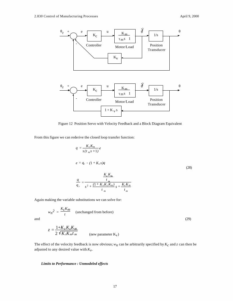
Damping Control in the Position Servo: Velocity Feedback The response of Fig 11 is not very satisfactory, especially if the major design criterion is settling time. The implication is that if a shorter settling time is desired, a new motor/load system must be specified, which negates one major benefit of control, that is altering the closed-loop system without the need for altering the process itself. To overcome this problem, it is necessary to gain access to the first order term of the characteristic equation for this system, since that term defines the system damping. 4 While there are several ways of motivating our approach, consider a simple physical argument. Damping is defined as a force acting in opposition to the motion and (if the system is linear) acting in proportion to the velocity. Thus damping is proportional to the negative of the velocity. Examining Fig 10, it is evident that if in addition to measuring and feeding back position, we as well measure and feedback (with a negative sign) the

velocity θ.. then we should add damping to the system. Thus we have modified the system as shown in Fig 12.

4 Notice that if we had such control, we could determine all of the coefficients in the characteristic equations, and thus could specify completely the system dynamics. In the theory of state-determined systems this is equivalent to having full state control, that is we can modify all the coefficients of the characteristic equations using feedback control. Such state feedback systems are typical of what is referred to as Modern Control Systems and represent a different approach to feedback control than discussed in this Chapter. For More information on State Feedback see: Ogata, Modern Control System Principles, Chapter 16 Kwakernak and Sivan, State Variable Control Systems


17


Kceθr u θ

1/sK mτm s + 1

+

-

Kv

Ýθ


Kceθr u θ

1/sK mτm s + 1

+

-

Ýθ

1 + K v s

⇓

Figure 12 Position Servo with Velocity Feedback and a Block Diagram Equivalent From this figure we can rederive the closed loop transfer function:

θ = K cKm

s (τm s + 1)e

e = θr − (1 + Kv s)θ

θθ r

=

Kc Km

τm

s 2 + (1+ K vK cKm )τ m

s + KcKm

τm

(28)

Again making the variable substitutions we can solve for:

ωn2 = KcKm

τ (unchanged from before)

and (29)

ζ = 1+KvKcKm

2 KcKmτm (new parameter Kv) The effect of the velocity feedback is now obvious; ωn can be arbitrarily specified by Kc and ζ can then be adjusted to any desired value with Kv.

Limits to Performance : Unmodeled effects


18

This design implies that any speed of response is possible, and indeed that is true, but only up to the power capabilities of the amplifier and motor combination, as mentioned earlier. To find the ultimate limit of this system, it is necessary to reexamine the assumptions made earlier. These include the simplified model of the motor, the modeling of the amplifier as “perfect” and the implication that the measurements were perfect and “noise-free”. In fact, both of these effects: model errors and measurement noise will be dominant limits when addressing any real system, and in particular when applying this theory to manufacturing processes. The effect of model errors is quite complex, and would require a more in-depth treatment of control theory. However, it is clear that if the process is modeled incompletely, then the design derived by the transfer function analysis given above will not produce the expected performance. However, it may produce acceptable performance over a specified range of operation. Defining this range is an important aspect of control system design, and some rudiments of this specification are covered below under the heading of frequency response. Most importantly, modeling errors can lead to stability problems, where the performance is not only different from expectations, but also unstable and potentially disastrous. Therefore, knowledge of stability analysis is also essential to control system design. Measurement error has a direct and easily quantified effect on the system. The controller can only regulate the system to the perceived output value, thus any measurement errors will be directly reflected into output errors under feedback control. The effect of noise is more subtle, and requires a closer definition of noise. First, we can characterize noise as any unwanted signal that does not relate to the actual physical variable being sensed. However, if this noise is a zero mean process, then it is often acceptable to assume that on average the noise signal is zero. In such a case the noise does not affect the mean value of the output, but only causes variations about that mean. If it is not zero mean, then it again produces a steady-state measurement error that cannot be averaged out by the control system.

Disturbance Rejection for the Position Servo Finally we must consider the basic problem of regulation, where the control objective is to maintain the output at the reference value in the face of unwanted disturbances. Borrowing from the velocity servo analysis, we can model the disturbance as shown in Fig 5, and then simply augment the block diagram of Fig 12 , as shown in Fig 13.


Kceθr θ

1/sK mτm s + 1

+

-

Ýθ

1 + K v s

1/Kt

Td

++

Figure 13 Position Servo with Torque Disturbance We again set the reference to zero and concentrate on deriving a disturbance transfer function, which not surprisingly (given Eqn 17) is found to be:


19

θ = Km

s (τm s + 1)− Kc 1+ Kvs( ) ⋅ θ + Td / K t( )

θTd

= ( Km / Kt ) / τm

s2 +(1+ KvK cKm )

τm

s +KcKm

τ m

(30)

As before we now find that the disturbance is reduced by a steady-state factor 1/KcKm, and that as the control gain Kc is increased, the effect of the disturbance is diminished. But why has it not been eliminated, since there is a “free integrator” in the loop, just as with the example in Fig 7 for the velocity servo?

Proportional - Integral (PI) Control This result indicates that the location of the disturbance and integrator in the loop is quite important, and suggests that to eliminate Td completely, we must again incorporate an Integrator into the controller. However, this time we will do so by adding the integrator to the controller rather than exchanging it for the proportional term. Thus, the controller block will be Gc = Kc + KI/s or a Proportional + Integral (PI) controller. PI controllers are quite common and are used precisely for the purpose of providing zero steady-state error to a system that is otherwise “OK”. With this new controller substituted into the block diagram of Fig 13, the disturbance transfer function becomes:

θTd

= ( Km / Kt ) /τ m

s2 + (1+ KvK cKm )τm

s + Km (K c + KI / s)τm

= s(Km / Kt ) / τm

s3 +(1+ K vKc Km )

τ m

s2 +Km Kc

τm

s +Km K I

τm

(31)

Since the numerator of Eqn 31 vanishes as s → 0, the PI controller has eliminated the steady-state effect of the disturbance. Since steady-state implies that s → 0, then in steady-state θ/Td = 0. Note also that all three coefficients in the characteristic equation can be adjusted independently using Kv, Kc, and KI. In addition to the error elimination, the familiar second order characteristic equation is gone, and we are faced with a third order denominator. How can we again decompose this equation into the familiar τ’s, ωn’s and ζ’s? In fact we simply determine the roots of the denominator and produce the factored characteristic equation: (s +p1)(s+p2)(s+p3) = 0 (32) where the roots p i can be real or complex. We know that at least one must be real (since comp lex roots must have conjugates), so there are two possibilities: all three roots are real: (s + p1)(s+p2)(s+p3) = 0 (33) or one real root and one pair of complex roots: (s + p1)(s2 + 2ζωn s + ωn

2) = 0 (34)


20

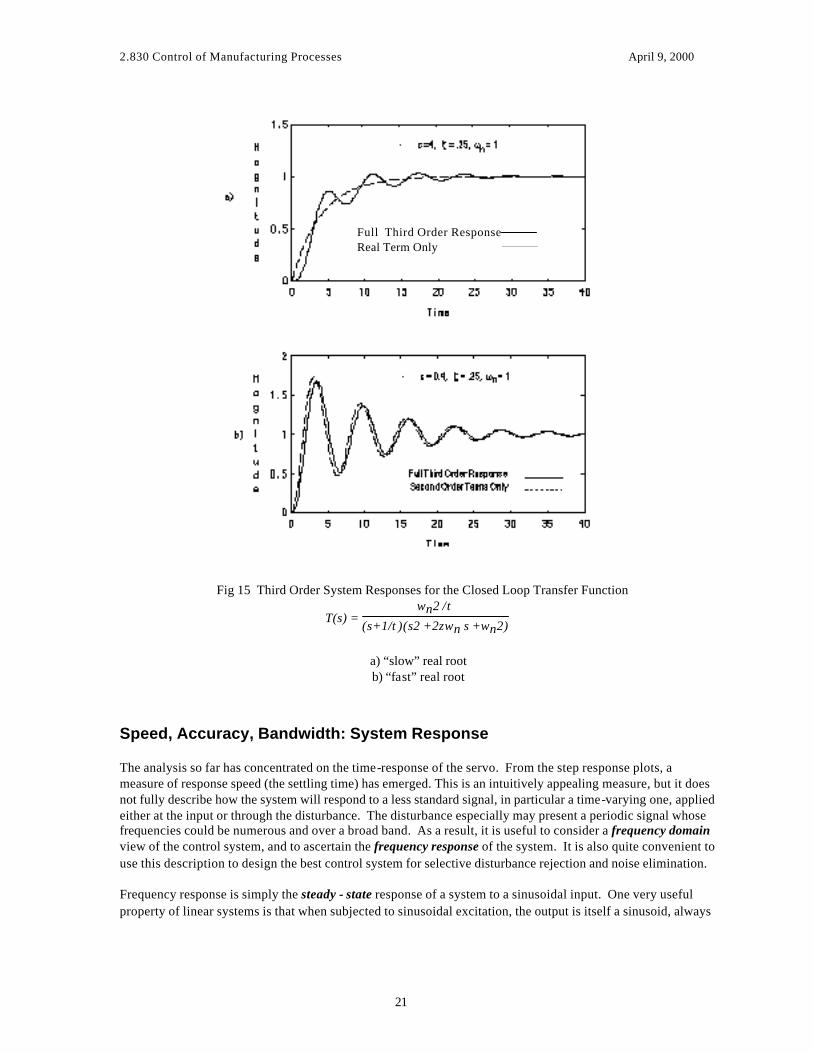
Detailed analysis of these roots is beyond this treatment, but we can speculate on expected responses. Linear system theory, and the Laplace Transform can be used to show that the response of these higher order systems will in fact be the sum of responses of each factor. The relative weight applied to each factor is a function of their relative speed and the nature of the numerator (which itself can have dynamic terms). Figures 14 and 15 illustrate this effect for Eqns 33 and 34. Note in 15 that when one of the roots is much larger than the others, its effect is negligible.

Fig 14 Third Order System Response with Real Roots


21

Full Third Order ResponseReal Term Only

Fig 15 Third Order System Responses for the Closed Loop Transfer Function

T(s) = ωn2 /τ

(s+1/τ)(s2 +2ζωn s +ωn2)

a) “slow” real root b) “fast” real root

Speed, Accuracy, Bandwidth: System Response The analysis so far has concentrated on the time-response of the servo. From the step response plots, a measure of response speed (the settling time) has emerged. This is an intuitively appealing measure, but it does not fully describe how the system will respond to a less standard signal, in particular a time-varying one, applied either at the input or through the disturbance. The disturbance especially may present a periodic signal whose frequencies could be numerous and over a broad band. As a result, it is useful to consider a frequency domain view of the control system, and to ascertain the frequency response of the system. It is also quite convenient to use this description to design the best control system for selective disturbance rejection and noise elimination. Frequency response is simply the steady - state response of a system to a sinusoidal input. One very useful property of linear systems is that when subjected to sinusoidal excitation, the output is itself a sinusoid, always


22

of the same frequency. However, the amplitude and phase of the output relative to the input is typically quite different, as shown in Fig 16, and it is this difference that provides a wealth of information about the system.5

Magnitude

φ

Time

Input sin(ωt) Output 0.75 sin( ωt + š/2)

Fig 16 Input Sine Wave and Linear System Output Notice that the output differs only in the magnitude and phase angle, but not the frequency

To analyze a system described by transfer functions, we make the substitution s = j ωω and then follow the rules of complex number algebra. Fortunately this need only be done for a few simple elements, and the rest of the analysis follows from combination of these simple elements. Consider again a simple first order system (e.g. the DC motor). The sinusoidal transfer function for such a system becomes:

G(s) s = jω = G( jω ) =

Kτ ⋅ jω + 1 (35)

In this jωω domain, the input is implied to be a sinuosoid of frequency ω and unity amplitude (although it can be scaled linearly to any value). Since G(jω) is a complex number, it can be described in terms of orthogonal components (real and imaginary parts) or in polar form, with a magnitude and phase angle. For G(jω) these two precisely describe the amplitude and phase of the response to a sinusoid. Thus for Eqn 35:

5 Proof of this analytically can be done by using the Laplace Transform. Consider the example of a first order

system G(s) = K

s+a . Taking the transform of the sine input: L( sin(ωt)) = ω

s2+ω2 . = R(s) . The output is

then found as C(s) = G(s) R(s) . Thus

C(s) = Kω

(s+a)(s2+ω2)

Using the inverse transform, the time response c(t) is given by:

c(t) = αe-jω t + αe+jωt + be-at Since our analysis is only for steady state, the first term vanishes, leaving us with a complex expression:

c(t) = αe-jω t + αe+jωt = β sin (ω t + φ) where α and β can be shown (see Ogata chapter 9) to be functions of the parameters of G(s) and the frequency ω.


23

G( jω ) =K

τ 2ω 2 + 1 (36)

∠G( jω ) = tan−1 Im (G)

Re(G)= − tan−1(τω) (37)

A quick look at Eqn 36 indicates that as the frequency of the input is increased, the output magnitude will decrease, and Eqn 37 indicates that the phase angle will be negative (a phase “lag”) and will become more negative with frequency. Since both |G| and ∠G are functions of ω, they can be plotted on similar scales to illustrate the effect of all values of frequency on the system. In addition, as will be shown later, it is best to plot both variables on a log ω scale and to plot log magnitude as well. The result is a Bode Diagram and Fig 17 shows a non-dimensional Bode Diagram for a simple first order system with K = 1 and τ = 1.

Fig 17 Bode Diagram for G(s) = 1

s+1

We can interpret this plot by looking at how the magnitude and phase change with ω. Notice that at very low frequencies |G| (often referred to as the “gain”) is unity and remains nearly at that level until near ω = 1/τ. Beyond ω = 1/τ, the gain drops off rapidly, eventually along a straight line of slope -1 on the log-log scale. Notice also that at low ω the phase is nearly zero, but as the point 1/τ is approached, the lag approaches -45o and eventually reaches an asymptote at -90o. The significance of the point 1/τ is more evident when considering asymptotic approximations to this plot. As shown on Fig 17, both the magnitude and phase plots are well approximated by straight-lines. For the gain these lines are in fact the low frequency and high frequency asymptotes. For the phase, the low and high frequency asymptotes are horizontal lines at 0 and -90o, and the phase change is well approximated by a line from 0o at ω = 0.1/τ to -90o at ω = 10/τ. Thus, knowing only the time constant of the transfer function, we can immediately plot the Bode Diagram using asymptotic approximations. Notice that any gain term (K) in the transfer function is applied as a simple vertical scaling of the magnitude plot, but has no effect on the phase. Now consider the second order underdamped system:

G(s) = ωn2

s2 + 2ζωn s + ωn2

Rewriting slightly, and making the substitution s = jω, the sinusoidal transfer function becomes:


24

G(jω) = 1

(1-ω2

ωn2)+ 2jζ ωωn

(38)

Again looking at magnitude and phase of this complex ratio:

G(jω) = 1

1- ωωn

2 2 + 2ζ ω

ωn

2

∠G(jω) = - tan-12ζ ω

ωn

1- ωωn

2

(39) A Bode Diagram for this transfer function is shown in Fig 18. As can be seen from the transfer function, as ω ⇒

0 again |G| ⇒ 1, and as ω ⇒ ∞, |G| ⇒ 1/ω2 , or a slope of -2 on the Bode Diagram. Again the major changes occur at ω = ωn, and the asymptotic gain plot shows that the change in slope from 0 to -2 occurs at that so-called break point . While the asymptotic plot is quite simple and appears identical to the first order plot, save for the increased slope, a closer look at the diagram shows the effect of the damping ratio. As the frequency approaches ωn , the magnitude increases and reaches a peak at a point near ωn (the point of resonance is

ω r = ω n 1− 2ζ 2 . While the asymptotic plot misses this effect, on either side of the resonance the agreement

is quite good. The phase also looks somewhat like a simple doubling of the first order case, and the asymptotic plot is simple a line from 0o at ω = 0.1ωn to -180o at ω = 10ωn . However, notice that the actual phase change becomes more severe as the damping ratio decreases.


25

|G|

φ

ω

-2ζ = 10.50.25

Fig 18 Bode Diagram for G(s) = ωn2

s2 + 2ζωns + ωn2

Basic System Characterization : Bandwidth How do plots of the frequency response help in design? There are many specific methods associated with the design of feedback control systems based on use of the Bode Diagram, but here we want only to introduce a few major concepts that will be useful when dealing with manufacturing processes. The first concept is that of bandwidth. Simply defined, the bandwidth is the range of frequencies over which the system response is “useful”. There can be many definitions of “useful”, but the most common is that the output is useful as long as it is greater than 0.5 to 0.707 times the input. While this may seem arbitrary, and an integer (such as one!) may seem more convenient, it is chosen because of the asymptotic character of most systems. Consider the simple first order system. The gain diagram shown in Fig 17 shows that if we chose |G|>1 as the definition, the bandwidth would also be zero, since the magnitude never actually reaches unity. However, if we choose 0.707, this point in fact occurs precisely at the break point where ω = 1/τ. Thus the bandwidth of this simple first order system is from 0 to 1/τ. Likewise, for our unity gain second order system shown in Fig 18, the bandwidth is well approximated by the range 0 to ωn . Notice that the bandwidth will in fact be variable depending upon ζ, and will be precisely equal to ωn only when ζ = 1.0 . To consider the real utility of the bandwidth measure, it is necessary to again look at a feedback system. For this we again turn to the servo example. The question arises: if we know the frequency response of the motor alone, what is the frequency response of the proportional speed servo of Fig 6 and how does Kc affect this response? The answer requires some complex algebra, which leads to a reduced solution.


26

General block diagram algebra on a closed-loop system, such as that shown in Fig 19, reveals that the closed-loop transfer function is given by:

T(s) = G(s)1+G(s)H(s)

and if H(s) = 1

T(s) = G(s)1+G(s) (40)

+

-

G (s)

H (s)

T (s)

Fig 19 A General Block Diagram and Equivalent Closed-Loop System To find the gain plot for the closed loop velocity servo, we need only substitute the appropriate transfer function, set s=j ωω , and then determine the magnitude. For the general closed-loop transfer function with unity H(s):

T(jω) = G(jω)1+G(jω)

T(jω) = G(jω)

1+G(jω)

≈ G(jω)1+G(jω) . (41)

The last expression, which is an approximation, makes the problem quite simple, since we already know the term |G| from the bode diagram. From Eqn 41 we can see that if |G| >>1, then |T| tends to 1, and as |G| approaches 0, |T| tends to zero. Finally, if |G| = 1 , then |T|≈ 0.5, which happens to be one measure of useful output from our bandwidth definition. In other words, if the open-loop transfer function gain |G| is much greater than one, the closed-loop gain |T| will always approach unity. Now to our servo problem. The G(s) (forward loop transfer function) for our servo is given by:

G(s) = KcKm

τms + 1

(42)


27

The Bode Diagram for this transfer function is simply that of Fig 17 scaled by the gains KcKm. The resulting gain diagram is shown in Fig 20 along with the corresponding plot for |T|. To determine the corresponding closed-loop bandwidth, we really only need to find the point at which |G| is unity. This is defined as the crossover point (or crossover frequency). Fig 20 shows the crossover point for KcKm = 10, but in principle Kc can be adjusted to any desired value. If we define the bandwidth of this closed-loop system , as the range over which the output is > 0.5, then it is clear that the crossover point (ωc) on the |G(ω)| plot corresponds to the closed-loop bandwidth ωb.

K Kc m

K K

10

0.1

K Kmc

c munity gain for KcKm = 10

bandwidth

ω

crossover frequency

Fig 20 Open-Loop / Closed-Loop Correspondence for a Velocity Servo

Thus the bode diagram for the open-loop system can be used directly, without further plotting or analysis, to determine the crossover frequency, which in turn tells us the closed-loop bandwidth.

Effect of Measurement Noise and Disturbances Returning to the simple velocity servo problem, consider the existence of noise in the feedback path, as shown in Fig 21, arising from the measurement process. This noise enters the loop in a manner similar to the input, so the noise transfer function is identical to the input-output transfer function. Therefore, the frequency response to noise in the measurement is the same as the closed-loop diagram in Fig 20. Now assume that the noise is characterized by the signal n(t) = sin(ωt). From Fig 20, it can be seen that if the noise frequency is less than ωb , the noise amplitude will be reflected to the output with no attenuation. However, if the noise frequency is greater than ωb , it will be attenuated by the factor 1/(ω−ωb). This leads to the well known conclusion that noise above the bandwidth of the system is usually not a problem (until we try to increase the bandwidth!) but noise within the bandwidth of the system is a major problem. The Bode Plot allows quick, graphical evaluation of noise rejection in this manner.


28

Kc-

Gp (s)

N (s)+

+

+Ωr Ω

Fig 21 Measurement Noise in a Velocity Servo If a disturbance enters the system, as shown in Fig 22, the

1/Kt

Td

++ Kc

+

- Gp (s)

Ωr Ω

Fig 22 Velocity Servo with a Disturbance disturbance transfer function can be found again from block diagram algebra as ( recall Gp = Km/(τms + 1) ):

ΩTd

=G p Kt

1+ Kc Gp (43)

The Bode Diagram for this transfer function could be drawn knowing only Gp and Kc, but we can in fact simply notice the difference between this expression and the closed loop transfer function

ΩΩ r

=KcG p

1 + Kc Gp

ΩTd

=1

KcK t

ΩΩr

(44)

Thus the disturbance frequency response is simply the closed loop response scaled by the factor (1/KcKt). Near zero frequency the rejection is (Km/Kt)/(1+KcKm) , which is precisely what was found earlier for the steady-sate disturbance rejection of this servo. Note that for this particular disturbance, which enters the system at the input to the plant, high frequency disturbances will be rejected, simply because the bandwidth of the motor itself (which is 1/τm) will prevent any high frequency inputs (such as the disturbance ) from propagating to the output.

Closed-Loop System Stability: Right-Half Plane Roots and Phase margin All of the systems discussed above have had clear and robust points of equilibrium. This can be traced to the analytical fact that the real parts of all the roots of the characteristic equations (which, recall, are the arguments of exponentials in the time response functions) were all negative. But what if through the use of feedback, which we know can alter the roots of the “new” closed-loop characteristic equation, one or more roots become zero or


29

positive. This implies that at least one exponential term in the time solution will diverge with time, and approach infinity. Such a condition would be unstable, and must be avoided. Not only can we use linear system theory to detect instability, we can also use it to develop a measure of proximity to stability limits, or the margin of stability. To illustrate the concept of root change and instability, consider the third order system developed earlier when PI control was applied to the position servo (Eqn 27). The characteristic equation for that system is:

s 3 +

1+KvKcKmτ

s 2 + KmKc τ

s+ K IKmτ

= 0. (45)

Assuming for the moment that Kc and Kv are fixed, and we will only vary KI, this can be simplified to: s 3 + a2 s 2 + a1 s+ K = 0 (46)

where K = KI Kmτ .

By solving for the roots of Eqn 46 as K is varied from 0 to ∞, and then plotting these on the complex or “s”-plane, the location of the roots for all possible values of gain can be easily seen. This plot, referred to as the root-locus for the closed-loop system, is shown in Fig 23, assuming the values shown for Kc Kv, and with Km = 1.0.

K=0

Breakaway point

Real

Imaginary

x x x

K=Kcritical

Figure 23 Locus of Roots in the s-Plane for the System of Eqn 42 with Kc = 2, Kv = 1, and τ = 1 To interpret this plot, recall that if a root is real, it has simple exponential response. Thus any root that lies on the abscissa has no complex part, and the magnitude represents 1/τ of a first order term in the response. Any


30

root that appears in the general s-plane has both real and complex parts, and is therefore an oscillatory root pair. The rate of decay of such terms is determined by the real-part of the root.6 With this rapid introduction to s-plane analysis, Fig 23 becomes more clear. At K = 0, we have essentially an open loop system and the roots are the roots of the open-loop block in the system. Note that the integrator appears as a root at the origin. As K is increased, these roots move in such a way that one always remains real (as expected) and the other two converge on the real axis and then “break” into the complex plane. Thus as the gain K is increased, a pair of complex roots develops. As K is increased further, the real root becomes faster and faster (and therefore less significant to the response) and the complex roots change by moving farther from the origin (ωn increasing) and by moving closer to the imaginary axis (settling time increasing). Finally, there is a critical gain at which point the complex roots lie on the imaginary axis. This implies zero damping or sustained oscillation for these roots. This point is called marginally stable. As K is increased, the roots move into the positive real half-plane (or right-half plane) and diverge, leading to an unstable system. The existence of any gain value that causes right-half plane roots indicates the potential for instability, and the proximity of roots to the imaginary axis is a measure of relative stability. The more negative the real part of the roots the more stable the system. This corresponds to the observation that the more negative the real part the faster the settling time. Thus relative stability and settling time are directly related. Stability can also be analyzed using the Bode Diagram. Proof of frequency domain stability is beyond the treatment of this text, and can be found in any of the texts listed in the bibliography at the end of this Chapter. However, an intuitive argument can be made to back up the analytical result. Consider a linear closed-loop system of high order (i.e. >2). Further assume that the phase lag of the forward loop transfer function G is exactly at -180o, and that |G| is exactly 1. The net effect of this is to make G appear like a simple negation block. This in turn cancels the negative sign at the summing junction, and we are left with what is known as a positive feedback system. Since errors will cause control actions that reinforce rather than diminish the error, positive feedback systems are unstable. Thus a critical point in the frequency response of the open-loop transfer function is that of unity gain and -180o phase. Proximity to this point is again an indication of a margin of stability. To illustrate this concept consider the third order system shown in Fig 24 (a simple 3 term real system) The Bode Diagram for this system can be easily constructed using graphical addition. Since the individual first order terms multiply together to form the Open-Loop transfer function G(s), they can be plotted individually on the Bode Diagram and then simply added. This is true for the magnitude since we use the log and it is true for the phase since multiplication of complex numbers in polar form requires addition of the angle terms.

Kc-

+ 1( s+ 1)( 5s +1)(10 s +1)

ΩΩr

Fig 24 Third Order System for Frequency Study

6 It can easily be shown as well that the distance from the origin to the complex root is ωn . Further, the angle this vector makes with the real-axis is defined as φ, then the damping ratio for the complex roots can be shown to be cos-1(φ).


31

The individual terms are plotted in Fig 25, and the sum of these is shown with the solid line. Most notable in this plot is the fact that the phase angle now goes from 0 to -270o . Based on the stability criterion stated above, this means that instability will occur, if the gain |G| were to be at or greater than unity when the phase <-180o . If the gain K in the system is raised (as indicated by downward motion of the unity gain line), then clearly this condition could occur at higher values of the gain. This is consistent with the root locus result in Fig. 23, which likewise indicated instability at higher values of control gain. Thus stability in frequency analysis relates to the proximity to a unity gain -180o phase condition. If the control gain of the system is adjusted such that this condition is avoided, then a stable, converging response is expected. Further, the margin of stability can be quantified in two ways: Phase Margin = φm = 180o + ∠G | |G| = 1 Gain Margin = K- |G|φ=-180 Thus by simple inspection of the Bode Diagram for any particular choice of control gain, we can ascertain the relative stability of the system. Phase margin is particularly useful since for a second order system it can be shown that ζ ≈ 0.01 φ , and this approximation is quite good even for system of higher order.


32

1s+11

5s+1

110s+1

Fig 25 Bode Diagram of the System In Fig 24

Effect of Measurement Delays

A prevalent problem in any manufacturing process is access to measurable outputs. In many cases a compromise must be made whereby measurements are taken some time after the output actually occurs. Quality Control sampling is an extreme example of this. In a faster time scale, measurements are often delayed by physical phenomena that intervene between the point of production and the point of measurement. In either case, a significant pure delay is introduced that can have a profound effect on the performance of the feedback system. To analyze this effect, it is most convenient to return to the Bode Diagram. A pure time delay term can be expressed in input-output terms as: y(t) = u(t-Td)


33

where Td is the delay time. In the s-domain this “block” can be expressed by the transfer function: Gd(s) = e-Ts (47) Now consider a simple velocity servo with a pure delay in the feedback loop, as shown in Fig 26. To develop the Bode Diagram for this system, we plot a first order term for the motor, and again represent Kc as a scale shift in |G|. To add the delay effect, we must first look at it in terms of gain and phase: Gd(s)|s=jω

= e-jωT = |G|e∠G

Thus |Gd| = 1

∠G = φ = -ωT (48) This tells us that a pure delay will introduce additional phase lag into the system, and rather severely so, since it is proportional to the frequency, and thus has no asymptotic value.

Kc-

+

e-Ts

K mτm s + 1

Ωr (s) Ω (s)I (s)

Fig 26 Velocity Servo with a Measurement Delay The Bode Diagram in Fig 27 shows the effect of a 0.1 sec delay term on the velocity servo. Without the delay we know that no stability limit exist for the velocity servo. Both our earlier analysis and the observation that the phase never goes below -90o proves this point. However, when the phase lag of the delay is added, it is apparent that above ω = 19 rad/sec the phase plummets below -180o and puts a firm limit on the maximum possible gain. From this diagram we can see that the critical gain Kcrit ≅ 20. It is also apparent from Eqn 48 that if Td increases, this limit will become even smaller.


34

0

-50

-100

-150

-200

1s+1

e -Ts1s+1

-180

e -Ts

ωω

Critical Gainwith Delay

e -Ts1s+1

Fig 27 Effect of a Pure Delay on Phase of a Second Order System


35

When the gain is limited so is the crossover frequency, which in turn limits the closed-loop bandwidth of our servo. Thus the most immediate effect of the delay on any system is to place a limit on the bandwidth that can be achieved. This in turn limits the speed of response. However, note that this also limits the amount of control gain that can be applied. Recalling that this gain directly affects the disturbance rejection and error characteristics of most systems, limiting the gain magnitude has the effect of impairing the disturbance-rejection and error-eliminating properties of the controller. While these problems can be mitigated using free-integrators, this in turn only adds more phase lag to the system 7.

7 A free integrator is essentially a first order system with zero time constant, and simple analysis shows that |G| = 1/ω and φ = -90o . Thus a free integrator adds a constant -90o of phase lag, thereby decreasing any phase margin and further limiting the potential bandwidth. Notice, however, that |G| ->∞ as ω->0, just as was shown to be necessary for zero steady-state errors.

Elements of Control

Documents

Transcript of Elements of Control