D O C U M E N T O

D E T R A B A J O

Instituto de EconomíaD

OC

UM

EN

TO d

e TR

AB

AJO

I N S T I T U T O D E E C O N O M Í A

www.economia.puc.cl • ISSN (edición impresa) 0716-7334 • ISSN (edición electrónica) 0717-7593

The Effect of Transport Policies on Car Use: A Bundling Model with Applications

Francisco Gallego; Juan-Pablo Montero; Christian Salas.

4322013

1

The Effect of Transport Policies on Car Use:

A Bundling Model with Applications

Francisco Gallego, Juan-Pablo Montero and Christian Salas∗

February 28, 2013

Abstract

In an effort to reduce pollution and congestion, Latin American cities have

experimented with different policies to persuade drivers to give up their cars in favor

of public transport. Borrowing from the bundling literature, the paper presents a

novel model of vertical and horizontal differentiation applied to transport decisions:

households differ in their preferences for transportation modes –cars vs public

transport– and in the amount of travel. The model captures in a simple way a

household’s response to a policy shock, i.e., how to allocate existing car capacity,

if any, to competing uses (peak vs off-peak hours) and how to adjust such capacity

overtime. Using few observables, the model is then used to analyze the effects of two

major transport policies: the driving restriction program introduced in Mexico-City

in November of 1989 –Hoy-No-Circula (HNC)– and the public transport reform

carried out in Santiago in February of 2007 –Transantiago (TS). The model’s

simulated effects are not only consistent with the econometric estimates in Gallego

et al (2013) but also help understand the mechanisms that explain them.

Key words: public transport, driving restrictions, pollution, congestion.

JEL classification: R41, Q53, Q58.

1 Introduction

Air pollution and congestion remain serious problems in many cities around the world,

particularly in emerging economies because of the steady increase in car use (EIU, 2010).

∗Gallego (fgallego@uc.cl) and Montero (jmontero@uc.cl) are with the Department of Economics ofthe Pontificia Universidad Católica de Chile (PUC-Chile) and Salas (csalaspauliac@worldbank.org) is

with the Development Economics Research Group of the World Bank. We thank seminar participants

at various places –including the Fifth Atlantic Workshop on Energy and Environmental Economics

at A Toxa (Galicia) in June of 2012– for comments and Enrique Ide for excellent research assistance.

Gallego also thanks financial support from Fondecyt (Grant No. 1100623) and Montero from the Spanish

Ministry of Economy and Competitiveness (Project ECO2009-14586-C02-01) and Instituto Milenio-Basal

SCI (P05-004F and FBO-16).

1

This trend has also contributed to increasing carbon emissions. Latin American cities

have experimented with different policies in an effort to contain such trend. In November

of 1989, for example, authorities in Mexico City introduced Hoy-No-Circula (HNC), a

program that restricted drivers from using their vehicles one weekday per week. More

recently, in February of 2007, authorities in the city of Santiago-Chile embarked in a city-

wide transportation reform, Transantiago (TS), with the idea of improving and increasing

the use of public transport. As shown in Table 1,1 other major efforts in Latin America

are of the same type, either driving restrictions or reforms in public transportation; there

is total absence, so far, of more market-oriented instruments such as road pricing and

pollution taxes.2

*** Insert Table 1 here or below ***

Have these policies been effective in persuading drivers to give up their cars in favor

of public transport, and hence, in reducing congestion and pollution? The problem with

evaluating these policies is that it is not always easy to construct a counterfactual against

which the performance of the policy can be contrasted upon (Small and Verhoef, 2007),

and more so if we are interested not in the immediate or short-run effect of the policy but

in its long-run effect, i.e., whether and how fast households adjust their stock of vehicles.

In this paper we develop a novel, yet simple, model of a household’s transportation-

decision problem that can serve as theoretical framework for empirical applications. The

model is then applied to HNC and TS for which we also make use of the empirical results

that are in our companion paper Gallego-Montero-Salas (2013); hereafter GMS.

The model distinguishes short from long-run impacts of a transportation policy that

can take different forms.3 In constructing the model we (partially) borrow from the

bundling literature (e.g., Armstrong and Vickers, 2010), so we capture in a simple way

the essential elements of a household’s problem which are the allocation of existing vehi-

cle capacity, if any, to competing uses (peak vs off-peak hours) and how that capacity is

adjusted in response to a policy shock. Households are both horizontally and vertically

differentiated: they differ in their preferences for transportation modes –cars vs public

transport– and in the amount of travel. Some households will find it optimal to pur-

chase the car-bundle (i.e., use the car for both peak and off-peak hours), others to rely

exclusively on public transportation (bus-bundle), yet others to "two-stop shop" (e.g.,

car for peak travel and buses for off-peak travel).4

1A description of the transport policies in the table can be found in Ide and Lizana (2011).2The political economy of this absence is beyond the scope of the paper but it is nevertheless an

interesting area for more research. Caffera (2010) touches on the issue but in the specific context of

pollution control from industrial sources.3Throughout the paper, we understand for short run the period right after a policy shock, say, first

month, and long-run as the time it takes most agents to adjust their stock of vehicles as a response to

the shock. In GMS we find that this adjustment period is no more than a year in the two applications

we study. There can be longer-run effects (e.g.,changes in agents location within the city) but our model

does not consider them.4Note that only the car-bundle comes with a discount because the same car can be used for both

2

One of the advantages of the model is that it can be calibrated and utilized for policy

simulations (including estimations of policy costs) using few observables at the city level,

namely, the fraction of households owning either none, one, or more cars, the share of

car trips at peak hours, the share at off-peak hours, and the ratio of peak trips over

off-peak trips (we also need to make an assumption about the distribution of horizontal

and vertical preferences in the population).

The model provides several results, which help interpret the empirical results found in

the literature and in particular in GMS. First, the model illustrates how little informative

the shot-run impact of a policy can be. Take a driving restriction policy, for example,

which the model captures with a reduction in vehicle capacity. The short-run impact (i.e.,

before any household has adjusted its stock of vehicles) is unambiguous and as expected,

at least qualitatively: a reduction in car trips during both peak and off-peak hours.

Depending on parameter values (e.g., price of cars), the long-run impact of the policy

can go either way, however. If cars are relatively expensive, the reduction in car trips can

remain in the long-run or even extend if enough households find it optimal to return their

cars. Conversely, if cars are less expensive (or because households decide to buy older

and cheaper cars to by-pass the restriction), the policy can result in an increase in the

number of vehicles in the long-run. Similar arguments apply to a public transportation

reform, which the model captures with a change in the variable cost of using public

vis-à-vis private transportation. Regardless of the direction of the relative price change,

its short-run effect on car use is likely to be small and hard to detect empirically.5 The

long-run effect, however, can be shown to be substantial in either direction.

Second, the model shows that policy impacts can vary widely among different income

groups, which is important for policy design and evaluation. It shows, for example, that a

driving restriction policy like HNC is likely to have its greatest impact in middle-income

groups, where households were more likely to buy a second car, and lower in high- and low-

income neighborhoods but for different reasons. High-income households have already

sufficient car capacity to cope with the driving restriction while only a few low-income

households own a car, and those that do, cannot afford a second one. A public transport

reform like TS that increases the cost of using public transport uniformly across the city

is also likely to have very heterogenous impacts: lowest among the rich that relies less

on public transport and highest among the poor.

The model also allows us to understand whether the effect of policy intervention on

car use vary depending on the hours of the day —peak vs off-peak hours. This distinction

is important when in the empirical application we are only able to estimate policy impacts

at peak hours. This is precisely what we do in GMS. The empirical evaluation of GMS

peak and off-peak travel.5Litman (2011) explains that cross elasticities between public and private transportation are very

low in the short-run (0.05) . Furthermore, the 2006 Origin-Destination survey for the city of Santiago

(EOD-2006 for its initial in Spanish), for example, shows that most of the (passanger) cars in the city

(799,811) must be already in use to cover an equivalent number of morning trips (706,518).

3

for HNC and TS are based on hourly observations of concentration of carbon monoxide

(CO), which are recorded by a network of several monitoring stations distributed over

the two cities. As discussed in GMS, CO is found to be a very good proxy for vehicle

use, particularly at (morning) peak hours, compared to alternative candidates like hourly

records of traffic flows and of other pollutants.6 Under stable meteorological conditions,

like before and around the morning peak, rapid increases in vehicle use (and in CO

emissions) are immediately reflected in changes in CO concentrations.

Finally, we use the model to compute transport costs that these policies have imposed

on households due to changes in the relative prices of the different transportation options.

From the magnitude of the CO results in GMS,7 it may appear that a large fraction of

households were able to accommodate, at a reasonable cost, to these policy shocks. The

model shows otherwise, that only a few did; hence, the costs inflicted by these policies

remain largely unchanged in the long run. The reason for this latter is that households

that decided to buy an additional (or first) car because of the policy were households

that before the policy were not that far from buying that additional (or first) car anyway

(they didn’t do it before because buying a car is a lumpy investment). In the case of

TS, these transport costs amount to approximately $120 million annually (in 2007 U.S.

dollars) or 9% of the value of the stock of vehicles in 2007 (in the case of HNC these

costs reach 5% of the stock value).

The rest of the paper is organized as follows. Section 2 describes HNC and TS in more

detail together with the empirical results of GMS. The bundling model is presented in

Section 3. Its application to HNC and TS —including the estimation of transport costs—

is in Section 4. We conclude in Section 5.

2 Two major transport policies

We start this section with a word on why we find it fruitful applying the model to HNC

and TS. As we explained below, there is not much controversy in that HNC and TS did

not succeed in persuading drivers to give up their cars in favor of public transport (there

is some about the timing and the magnitude of the impacts; something this paper and

GMS contribute to as well). Yet, both policies are most valuable for the purposes of

understanding how households respond to these transport policies. These are policies of

6Mobile sources, and light vehicles in particular, are by far the main emitters of CO –97% and 94%,

respectively, at the time HNC and TS were implemented. Another reason to focus on CO is that it

allows us to study the response of different income groups by looking at the evolution of CO records

from individual monitoring stations which happen to be located in neighborhoods of disparate incomes.7For HNC, GMS find a statistically significant 13% reduction of CO in the short-run (i.e., first month)

and an 11% increase in the long-run. The length of the adjustment phase, i.e., the time it takes for the

policy to reach its long-term effect, is estimated to be about a year. As for TS, they find no impact in

the short run and a 27% increase in the long run, which is reached about 7 months after implementation.

All estimates correspond to (morning) peak hours and at the city level. Estimates at the county level

come below.

4

different nature and implemented in different cities, almost 18 years apart, which makes

it interesting to contrast the way households responded to them. More importantly, they

amount to one-time drastic interventions like no other in Latin America.

2.1 HNC in Mexico-City

HNC was established on November 20 of 1989, as a response to record levels of air pol-

lution and congestion in Mexico-City (Molina and Molina, 2002). The program banned

every vehicle –except taxis, buses, ambulances, fire trucks and police cars– from driving

one weekday per week, from 5am to 8pm, based on the last digit of its license plate

(GDF, 2004). The program was implemented all at once and the low cost of detecting

non-compliers, the heavy fines, and high police control resulted in near universal com-

pliance (Onursal and Gautam, 1997; Eskeland and Feyzioglu, 1997; Davis, 2008). The

program did not experience any relevant changes for the next two years (see GMS). In

contrast, other driving restrictions in Latin America (see Table 1) have affected only a

fraction of drivers (e.g., those using older cars) and under special circumstances (e.g.,

days of unusually high pollution).8

There is still the issue of whether some households could have moved forward the

purchase (and use) of an additional car to right after the announcement of HNC (No-

vember 6) or even before that in anticipation of a possible increase in car prices because

of HNC. There are several reasons to believe this should not be a concern, namely, that

the initial announcement of HNC had the program lasting until the end of February

(and only then, the program was officially made permanent), that the effect of HNC on

the stock of vehicles seems to have been rather modest,9 and that there was not much

time between the announcement and implementation so at best only very few households

could have adjusted so quickly.

Some believe that HNC had a good start (e.g., Onursal and Gautam, 1997; GDF,

2004),10 but most agree that over the longer term it lead instead to an increase in the

number of vehicles on the road (e.g., Eskeland and Feyzioglu, 1997; Ornasul and Gautam,

1997; Molina and Molina, 2002; and Davis, 2008). This mixed story is consistent with the

empirical findings of GMS. Their empirical strategy to obtain an estimate of the effects

of HNC on car use is to compare CO concentration levels two years before and after

policy implementation for some specific hours of the day (i.e., peak hours and off-peak

hours) and different income groups. Results at the city level show statistically significant

reductions of CO in the short run (i.e., first month) of 13% and 9% for peak and off-peak

hours, respectively. For the long run GMS find an increase of 11% during peak hours

8The driving restrictions in Medellín and Quito also appear quite comprehensive (e.g., Cantillo and

Ortuzar, 2011).9According to GDF (2004), of the total number of new cars sold in Mexico in 1990, 44.1% went to

Mexico-City as opposed to 45.6% in 1989 and 46.5% in 1988.10Davis (2008), however, argues that even right after implementation HNC failed to lead to pollution

reduction. More on this is in GMS.

5

and of 9% during of off-peak hours. Estimates for weekends show no reduction in the

short-run, as expected, and a significant increase in the long run of about 20%.11 The

length of the adjustment phase, i.e., the time it takes for the policy to reach its long-term

effect, was estimated to be between 8 to 125 months after implementation.

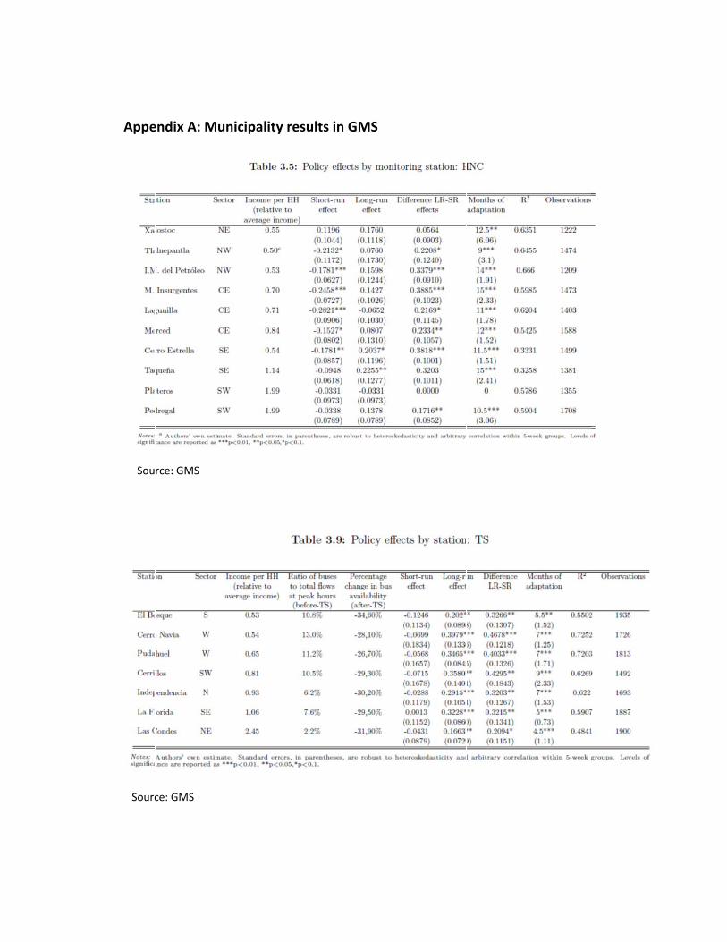
Using CO records at various monitoring stations, which happen to be located in

counties with households of different income levels, GMS are also able to estimate how

policy responses vary with income. Their results are reproduced in Appendix A (Table

3.5 of their paper). They find that HNC had its largest impact in middle-income groups,

where households were more likely to buy a second car. For example, for the municipality

of Cerro Estrella they find a short-run reduction of 18% (in peak hours) and a long-run

increase of 20%. The impact is much lower in high- and low-income neighborhoods for

the reasons explained in the introduction. For example in the poor Xalostoc GMS failed

to find any effect of the policy while in similarly poor Tlalnepantla, in the North-West,

they only find a short run effect; a reduction of 20%. On the other hand, in the richer

municipalities of Plateros and Pedregal, in the South-West, GMS did not find short run

effects and only mild increases in the long-run for the latter.

2.2 TS in Santiago-Chile

Nearly 18 years later, on February 10 of 2007, Chile’s government implemented Transan-

tiago (TS), with a similar motivation than HNC, that of persuading drivers to give up

their cars, but with a different instrument: improving, supposedly, the quality of public

transport. The old public transportation system was regarded as highly polluting, un-

safe, and inefficient both in terms of travel time and cost (e.g., Briones, 2009; Muñoz et

al, 2009).12 TS was intended to remedy these problems at once and for the entire city. It

involved a significant and sudden reduction in the number of buses, from roughly 7500 to

5500,13 and a radical (centrally-planned) change in the design and number of routes more

in line with a hub-and-spoke network where the existing subway system would play the

role of a hub. The other public transport reforms in Table 1, most notably Transmilenio

in Bogotá, have been more limited in scope and introduced gradually.

While the original design of TS was expected to deliver significant reductions in

congestion and pollution from fewer cars on the street,14 its actual implementation has

11Note that this 20% increase comes close to the 24% net increase at peak hours (from -13% to +11%)

and the 18% increase at off-peak hours. These net increases are all statistically significant at 1%.12Most bus routes passed through the central business district connecting terminal points on the

pheriphery, with average length of more than 60 kms (counting both directions), so most passengers

could travel almost anywhere in the city without transfers. Under TS, passengers are expected to

transfer a few times before completing their journeys (Muñoz et al., 2009).13See Briones (2009) for more details. More importantly for our analysis, the share of public trans-

portation on CO emissions is only 3% (CONAMA, 2004), so such a reduction in the number of buses

has virtually no effect on CO concentrations.14DICTUC (2009) estimates that TS, as conceived by its architects, would have reduced CO concen-

trations by 15% by 2010.

6

been recognized by many as a major policy failure (e.g., Briones, 2009) resulting in a

significant and permanent increase in the cost of using public transport from the first day;

which is what we exploit in our analysis of household behavior.15 GMS provides numbers

illustrating the extent of the intervention. Commuting time increased, on average, from

77 to about 90 minutes (both ways), mainly because of the increase in the average

travel time of public transport that went up by about 30% (from 102 to 133 minutes).

In contrast, travel time of cars and taxis does not seem to have been affected nearly

as much. The issue of anticipation to TS does not arise here despite its launch was

announced several months in advance; this is simply because nobody anticipated the

final outcome.

This deterioration in quality should have resulted in a switch towards alternative

modes of transportation, e.g., cars, and hence, in an increase in CO emissions. This is

precisely what GMS report using the same empirical strategy described above. Results

at the city level find no impact on CO in the short run (for peak hours) and a 27%

increase in the long run (also for peak hours). This long-run impact is reached about 7

months after implementation. Like with HNC, GMS also find that policy responses vary

significantly with income (their results are also reproduced in Appendix A). While the

short-term impact is found to be negligible in all parts of the city, the long-term impact

is found to be decreasing with income from a high of about 40% in the poorest areas

(e.g., Cerro Navia) to 17% in the richest county.

3 A model of car ownership and use

Can theory explain the empirical findings of GMS for HNC and TS? In particular, can

the long-run increase in CO be simply explained by more cars on the street or also by

dirtier ones and/or more congestion? Can impacts at peak in TS be consistent with

no impacts at off-peak (given that GMS could not estimate them)? Can differences in

income lead to such different effects? Do most households adjusts to these policies in the

long-run, or only a few? Can we obtain an estimate of the short- and long-run transport

costs inflicted by the policies using few observables like changes in the stock of cars?

To answer these and other questions, we develop a model that captures in a simple

way two essential elements of a household’s problem which are the allocation of existing

vehicle capacity, which is lumpy, to competing uses (peak vs off-peak hours) and how

that capacity is adjusted in response to a policy shock. The model is flexible and simple

enough to accommodate to all sorts of policy interventions and income groups.16

15The Economist (Feb 7th, 2008) referred to TS as "...a model of how not to reform public transport."16The model abstracts from longer-run considerations such as migration from and to the city.

7

3.1 Notation

There is a continuum of agents (households) of mass 1 that decide between two modes of

transportation –polluting cars and public transport (e.g., buses)– to satisfy its demand

for travel during both peak and off-peak hours (we will often refer to peak demand as

high () demand and off-peak demand as low () demand). Households differ in two

ways: in their preferences for one mode of transportation over the other (horizontal

differentiation) and in the quantity of transportation (e.g., kms traveled, number of trips)

they wish to consume (vertical differentiation). Horizontal preferences are captured with

a two-dimensional Hotelling linear city. A household’s horizontal preferences are denoted

by ( ) ∈ [0 1]× [0 1], where is the household’s distance to the car option for peakhours and is the distance to the car option for off-peak hours. This same household’s

distance to the bus option is (1 − 1 − ). The density of ( ) is ( ).17

Furthermore, the product differentiation (or transport cost) parameter is for the peak

and for the off-peak. A household’s vertical preferences are captured with inelastic

travel demands which are denoted by ( ) ∈ [0 1] × [0 1], where and are the

household’s number of (weekly) trips at peak and off-peak hours, respectively.18 The

density of ( ) is denoted by ( ).

A household is assumed to have a choice of owning zero, one, or two vehicles. Unlike

public transportation (buses), private transportation comes with a capacity restriction

that depends on the stock ∈ {0 1 2} of vehicles owned by the household. A householdthat owns a single vehicle ( = 1) has 1 trips available to be shared between peak and

off-peak hours.19 In turn, we assume that a household that owns two vehicles ( = 2)

faces no capacity constraints.20 The unit cost of using a car during peak hours is and during off-peak hours is . The unit cost of taking a bus is

for = . These

costs depend on congestion (i.e., aggregate car travel), and agents correctly anticipate

that, but we do not need to be explicit about them in this model because we are only

interested in the price difference, i.e., ∆ ≡ − for = , which simplifies the

analysis greatly.21

17Obviously this function may depend on income, but this is immaterial for what follows unless we

believe policies can directly affect (·), which we do not. They could, for example, if a policy introducespublic transport in a place where it was absent before. But here we interested in changes in the quality,

i.e., price, of an existing system.18The model can be easily extended, at the cost of additional notation, to elastic demands, e.g.,

() = () for = and with ∈ [0 1].19Because of this capacity constraint, think of and as weekly quantities. This would accomo-

date, for example, a household with a single car that on a daily basis alternates its use between peak

(commuting to work) and off-peak (shoping).20Note that to study the impact of a driving restriction we cannot simply let ∈ {0 1} since houselholds

that already own a car may either want to buy an additional one or return the one they have.21Take, for example, a transport policy that improves public transportation and, as a result, it also

alleviates congestion. Our model captures these changes as reductions in both and . However, given

the structure of the model, the household only cares about ∆. Note also that this formulation easily

accommodates the fact that car trips are generally longer (or more numerous) than bus trips. In other

8

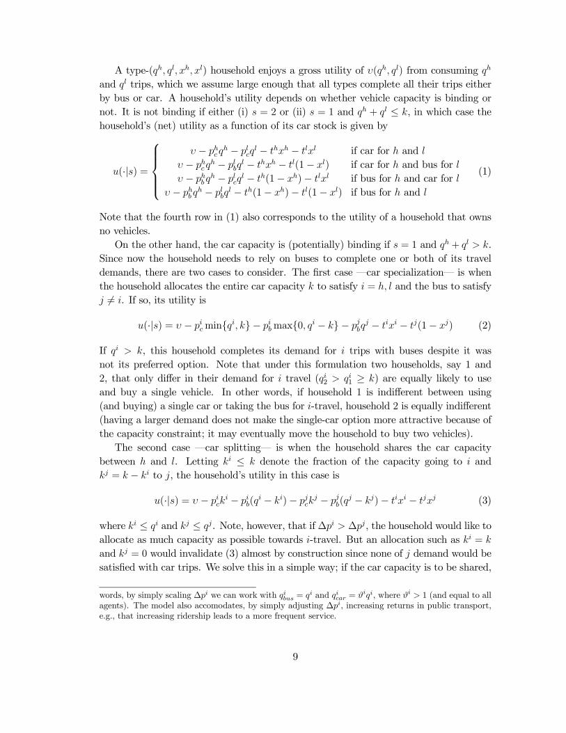
A type-( ) household enjoys a gross utility of ( ) from consuming

and trips, which we assume large enough that all types complete all their trips either

by bus or car. A household’s utility depends on whether vehicle capacity is binding or

not. It is not binding if either (i) = 2 or (ii) = 1 and + ≤ , in which case the

household’s (net) utility as a function of its car stock is given by

(·|) =

⎧⎪⎪⎪⎨⎪⎪⎪⎩ −

− − − if car for and

− −

− − (1− ) if car for and bus for

− −

− (1− )− if bus for and car for

− −

− (1− )− (1− ) if bus for and

(1)

Note that the fourth row in (1) also corresponds to the utility of a household that owns

no vehicles.

On the other hand, the car capacity is (potentially) binding if = 1 and + .

Since now the household needs to rely on buses to complete one or both of its travel

demands, there are two cases to consider. The first case –car specialization– is when

the household allocates the entire car capacity to satisfy = and the bus to satisfy

6= . If so, its utility is

(·|) = − min{ }− max{0 − }−

− − (1− ) (2)

If , this household completes its demand for trips with buses despite it was

not its preferred option. Note that under this formulation two households, say 1 and

2, that only differ in their demand for travel (2 1 ≥ ) are equally likely to use

and buy a single vehicle. In other words, if household 1 is indifferent between using

(and buying) a single car or taking the bus for -travel, household 2 is equally indifferent

(having a larger demand does not make the single-car option more attractive because of

the capacity constraint; it may eventually move the household to buy two vehicles).

The second case –car splitting– is when the household shares the car capacity

between and . Letting ≤ denote the fraction of the capacity going to and

= − to , the household’s utility in this case is

(·|) = − − (

− )− −

(

− )− − (3)

where ≤ and ≤ . Note, however, that if ∆ ∆, the household would like to

allocate as much capacity as possible towards -travel. But an allocation such as =

and = 0 would invalidate (3) almost by construction since none of demand would be

satisfied with car trips. We solve this in a simple way; if the car capacity is to be shared,

words, by simply scaling ∆ we can work with = and = , where 1 (and equal to all

agents). The model also accomodates, by simply adjusting ∆, increasing returns in public transport,

e.g., that increasing ridership leads to a more frequent service.

9

it is done proportional to the demands, i.e., = ( + ) for both = .22

In deciding whether to own zero, one or two vehicles the household solves

max{max(·|)− } (4)

where max(·|) is the utility from the best (short-run) transportation mix for a given

stock ∈ {0 1 2} and is the cost of buying a car, which can be made endogenous to thepolicy.23 Implicit in (4) is the assumption that households constantly adjust their stock

of durables to their optimal level while in reality liquidity constraints and/or transaction

costs may create a range of inaction where agents do not adjust their stocks at all (e.g.,

Eberly, 1994).24 We will come back to this issue below.

3.2 Short and long-run choices

We now compute a household’s optimal use and ownership choices.25 The structure of

the model allows us to conveniently sequence the analysis from vertical preferences to

horizontal preferences. We can first segment households on their likelihood of buying

one or two vehicles from looking at their demands and ; then we can tell which of

these households will indeed buy and use the vehicle(s) from looking at their horizontal

preferences and .

Consider first households with + ≤ . These households, those in group A

in Figure 1, will at best consider buying and using a single vehicle; the ones that do

are shown in Figure 2(a) (for now, ignore the dotted lines in both Figures 1 and 2 and

the ’s in Figure 2). As in any (multi-product) bundling problem, some consumers

will choose to consume both products ( and travel) from the same "supplier" (car

or bus), i.e., "consume the bundle", while others will choose to consume from both

suppliers. Figure 2(a) consolidates in one place both household’s long- and short-run

choices. All households with ≤ () ≡ 12 + ∆2 would rather use the car

than the bus for -travel (provided they have one available). And all households with

≤ −2 ≡ (), buy a vehicle despite it will only be used for -travel, i.e., despite

() ≡ 12 +∆2. There is fraction of households with weaker preferences

for cars, i.e., for = , which also buy the car because of the "bundle

22We are informally saying that there may be decreasing marginal benefits in car use that justify an

interior (splitting) solution. This latter is more reasonable if ∆ is not too far apart from ∆ , which

is what we find in the calibrations.23Note that if min{ }, households with strong preferences for cars, say = 0 or = 0, would

buy a car even if = ≈ 0.24Transaction costs may come from sales fees, sales taxes, search costs or the lemons problem afflicting

used vehicles.25Note that if ∆ = ∆ = 0, = 0 and ( ) ≡ 1, only 50% of trips will be made on cars.

10

discount" associated to it. The car-bundle discount is exactly equal to .26

*** Insert Figures 1 and 2(a) here or below ***

We can now use Figure 2(a) to illustrate the short and long run effects of a public

transport reform like TS. Suppose the policy means a slight deterioration of the quality

of public transport during peak hours, which can be captured by an increase in ∆

of some small amount , as illustrated by the dotted line in the figure (note that consid-

eration of a small amount is only to facilitate the exposition). Unlike households that

buy (and use) the car-bundle, households that only use the car for -travel (the "two-stop

shoppers" of the bottom-right corner) have spare car-capacity that is ready to be used

for -travel. Hence, there is an immediate (i.e., short-run) increase in car trips (and

pollution) during peak hours from households in group A equal to

∆() ≡

ZZ

1(

)( ) =

Z0

−Z0

1(·)(·) 0

where 1 (see the figure) is given by

1(

) =

Z ()

0

(() ) (5)

If the policy shock is permanent, there is an extra increase in car trips from additional

car purchases, so the long-run effect of the policy upon group A during peak hours is

equal to

∆() ≡

RR(

1 + 2 +

3)(·)

where 2(

) is given by an expression similar to (5) and 3 by

3(

) =

Z ()

()

¡() + [()− ]

¢

But because the policy also moves some households from the bus-bundle to the car-

bundle, there is a long run effect during off-peak hours as well (despite the price of public

transport has not changed there), which is equal to

∆ () ≡

RR

3(·)

Consider now households with + . There are four cases to study: groups

B, C, D and E in Figure 1. Like those in group A, households in group B buy at most

26The (long-run) purchasing cost of consuming car for -travel only is −∆ while for both and

travel is −∆ −∆. The "bus-bundle" does not come with any discount.

11

one vehicle, ∈ {0 1}, because and are, either individually or together, not large

enough to justify the purchase (and use) of two vehicles. It does not pay to buy two

vehicles for multiple use if (·| = 2) ≤ (·| = 1), or more precisely, if

2 −∆ −∆ ≥ −∆ −∆ (6)

where = ( + ) for = . Note that if ∆ ≈ ∆ = ∆, then (6) reduces

to + ≤ + ∆: It only pays to buy a second (multi-purpose) car if the saving

∆( + − ) more than offset the cost . The equivalent of (6) for a (single-purpose)

vehicle is ≤ + ∆ (see Figure 1). The fraction of households in group B that

effectively end up buying and using the car is shown in Figure 2(b). Note that the

car-bundle discount continues to be despite the capacity constraint.

*** Insert Figure 2(b) here or below ***

More interestingly, we can now use Figure 2(b) to illustrate the short- and long-run

effect of a second type of policy intervention: a driving restriction like HNC. Suppose

the policy reduces car capacity by a small amount (again, we restrict attention to

small changes just to facilitate the exposition).27 There are three short-run effects. The

first is the drop in car trips from households that use (and continue using) the car at

full capacity, i.e., those that consume the car-bundle. The second short-run effect, which

is captured by the horizontal dotted line in the upper-left corner in the figure, is the

reduction of car trips during off-peak hours from households that no longer consume the

car-bundle. This drop amounts toRR

(∆2)

1(·). Similarly, the thirdshort-run effect, which is captured by the vertical dotted line in the lower-right corner,

is the reduction of car trips during peak from households that no longer consume the

car-bundle and is equal toRR

(∆2)

1(·).The driving restriction can also have an additional and "positive" effect on car travel

in the long-run upon this group. For some households owning a car is no longer that

attractive (although using it is, provided the car is available). In fact, if the resale price

of a car is still , a fraction of households in B would sell their cars, and hence, reduce

their car trips, in both peak and off-peak, byRR

(∆2)(

2 + 3)(·)

andRR

(∆2)(

2 + 3)(·), respectively.28 However, if these households

face a transaction cost equal to

≥ ∆

(7)

none of these additional long-run benefits will accrue since no household will return a car

at a resale price of (1− ).

Note that the presence of a transaction cost introduces an option value to the

27Note that a large reduction in can also affect ∆ from changes in congestion (but we omit that

here).28Note that 3 and 3 are related by ∆

3 = ∆3

.

12

decision to invest in a car if households assign some probability to the possibility that

either kind of policy is canceled in the future or substantially changed. This was to some

extent the case in both HNC and TS. In the case of HNC, it was not clear at the time

of implementation whether the authority would mantain the program after the winter

months and in the case of TS some people thought that its bad start would only be

temporary (after a month or two people realized that it was not). As formally shown

in Appendix B, the introduction of an option value to the problem does not change our

analysis in any fundamental way; it only makes investing in a car less attractive (i.e.,

the cost of a new car is plus the cost of "killing" the option; is a parameter that we

calibrate so you may say that the cost of killing the option is included in it).

That the driving restriction reduces car travel (in the short-run and potentially in

the long-run) extends to all other households in group B except to those close to the

border + = − ∆. As captured by the (downward) sloping dotted line in

Figure 1, these households now belong to group C, so some of them will find it attractive

to increase the size of their car-bundle and buy a second car; not only by-passing the

driving restriction altogether but what is worse, increasing car travel during both peak

and off-peak hours.29 Figure 2(c) distinguishes precisely those households in group C

that buy two vehicles from those that buy one and from those that buy none (to simplify

the exposition, the figure focuses on the case in which ≥ , say, subgroup C1).30

In this case the bundle discount is not longer but ∆( − ) +∆( − ). This is

because households that want the car only for -travel do not buy two vehicles but just

one.

*** Insert Figure 2(c) here or below ***

The dotted line in Figure 2(c) depicts the effect of the driving restriction on group C1.

The short-run effect is simply the drop by the amount of car trips from the two-stop

shoppers. The long-run effect can be divided in two parts. The first corresponds to the

two-stop shoppers that would like to sell their cars if the resale price were to remain at

; if so, this would reduce car trips byRR

1(∆2)

2(·) during peak andbyRR

1(∆2)

2(·) during off-peak. And the second part corresponds totwo-stop shoppers that buy a second car; not only by-passing the driving restriction for

their trips but now also using the car for all of their trips. This increase in car trips

amounts toRR

1(∆2)

1(·) during peak andRR

1(∆2)

1(·)during off-peak. This is by far the most adverse effect of a driving restriction.

As shown by the horizontal and vertical dotted lines in Figure 1, this adverse effect

extends to households in group C that now belong to group D; a group in which house-

holds own either two vehicles, one or none. As shown in Figure 2(d), the difference with

group C is that some households in group D may buy two cars just for -travel (again, the

29Note that the same inward shift of the border + = + ∆ would happen with a policy

intervention that increases both ∆ and ∆ by .30There are three more subgroups: C2, where ; C3, where and ≥ ; and C4, where

≥ and .

13

figure focus on the case in which ≥ + ∆ and ≤ + ∆, say, subgroup

D1).31 The effect of the driving restriction policy on the two-stop shoppers that have one

car is the same as on the equivalent two-stop shoppers in C1. Finally, there is the group

of households, group E, that because of their large demands own either two vehicles or

none. As shown in Figure 2(e), these households never face capacity restrictions (shortly

we will come back to the dotted lines in the figure).32

*** Insert Figures 2(d) and 2(e) here or below ***

4 Application to HNC and TS

We first calibrate the model for both cities using ex-ante (i.e., before the policy) infor-

mation on car ownership and use and then proceed to answer the questions posed in the

previous section; in particular, can theory make sense of the empirical findings of GMS?

4.1 Calibration

We first calibrate the model to parameter values that reflect the ex-ante (i.e., before

the policy) situation of each city in terms of car ownership and use. The car-ownership

information includes the fraction of households that either own no cars ( = 0), one car

( = 1), or two (or more) cars ( = 2). The car-use information, on the other hand,

includes the share of car trips at peak hours (), the share at off-peak (

), and

the ratio of car trips at peak over car trips at off-peak (). The ex-ante information

is summarized in the first half of Table 2.33 In all numerical exercises, we assume that

households’ preferences are drawn from uniform distributions, i.e., ( ) = ( ) ≡1. The bottom half of Table 2 presents the calibration parameters obtained for each

city.34 The differences we observe are for the most part expected; for example, the higher

use of cars in Santiago is consistent with a higher and lower .

*** Insert Table 2 here or below ***

31There are three more subgroups: D2, where ≥ + ∆ and ; D3, where ≥ + ∆

and ≤ + ∆; and D4, where ≥ + ∆ and .32Note that the bundle discount for these households is 2 since they would buy two cars even if they

are to be used only for -travel.33The ex-ante information for HNC was obtained as follows: car-ownership from INEGI (1989),

fromMolina and Molina (2002, p. 227), and from the EOD-2007 for Mexico-City. In the absence

of more information, and based on what we know from EOD-2007 for Mexico-City and EOD-2006 for

Santiago, we also assumed for HNC that =

. All the ex-ante information for TS was

obtained from the EOD-2006 for Santiago.34We used the same initial values in both calibrations: ∆ = ∆ = = = = 2 = 1.

14

4.2 Policy simulations

As a first simulation exercise with the calibrated model, let us replicate the empirical

findings of GMS for HNC by decreasing car capacity to 020 (all the other parameters

remain unchanged). As shown in the first row of Panel A of Table 3, this HNC-like

policy leads to a short-run decline in car use during peak hours (∆) equal to the 13%

reduction in CO concentrations found by GMS. The short-run decline at off-peak (∆ )

is a bit higher than the empirical estimates, but the most striking results are the long-run

numbers (∆= ) which are far from the empirical estimates (increases of CO of 11 and

9%, respectively). The long-run inconsistency can be explained by two assumptions in

exercise A1 that are unlikely to hold in practice. First, in A1 all households have the

option to return their cars at the original price (according to the change in the stock of

vehicles shown in the last columns of A1 and A2, households would like to return 133%

of the current stock). If instead we assume that transaction/lemon costs are such that no

household returns its car(s), i.e., eq. (7) holds, exercise A2 shows that in the long run the

policy leads to a net increase in the stock of vehicles of 41%, although still accompanied

by a minor decline in car use (e.g., −27% in peak hours).

*** Insert Table 3 here or below ***

The second assumption in A1 is that the additional stock is equally polluting (and

fuel-efficient) as the existing one, which we know from Eskeland and Feyzioglu (1997)

is unlikely for HNC because of the import of older cars from adjacent regions. Thus,

if we also let the additional stock be 2.4 times as polluting (and less fuel-efficient) as

the existing ones,35 the results in ex. A3 match GMS long-run empirical estimates,

which illustrates that they are consistent with the theory once we incorporate these more

realistic assumptions. Even though the short-run gains are for most part undone, these

exercises show for the case of HNC that this is much less due to increases in car use and

congestion (actually they hardly changed with respect to the pre-HNC levels) than to

the entry of older and more polluting cars.

Let us now use the model to study the response of different income groups and see

how they match the empirical findings of GMS (which are reproduced in the Appendix).

We can do this by simply varying –which can be interpreted more generally as the

price of cars relative to household income– so as to match ex-ante car use in different

municipalities. Exercise A4 extends A3 to a higher-income neighborhood ( = 025) that

exhibits an ex-ante car use of 70% during peak () and 74% during off peak (

).

The effect of the policy is unsurprisingly small compared the city average in A3 because

these households have already sufficient car capacity to cope with the driving restriction

35Based on Betaon et al (1992), who find that each additional year increases CO emissions by approx-

imately 16%, a factor of 2.4 would suggest that the additional vehicles are on average 6 years older than

the fleet average, which is perfectly reasonable since 8% of the gasoline fleet in 1989 is at least 20 years

old (Molina and Molina, 2002).

15

(the long-run numbers go down to 0.6 and 0.7%, respectively, if we let the additional

cars in this higher income neighborhood be equally dirty than the fleet average). In turn,

exercise A5 looks at the other extreme by extending A3 to a lower-income neighborhood

( = 13) that exhibits an ex-ante car use of only 4%. The effects of the policy are again

intuitive since these are households that at most have one car, so the driving restriction

hits them hard in the short-run and only a few of them can afford a second car in the

long-run. One reason the empirical estimates in poor Xalostoc do not reflect the large

reduction of car use in the short run is partly because cars contribution to CO in such

poor areas is likely minor relative to the contribution of other sources not affected by

HNC (i.e., taxis, buses).36

We move now onto TS. Recall that the model captures a TS-like policy with changes

in ∆ and/or ∆. The first exercise in Panel B of Table 3 (exercise B1) considers a

TS-like policy that inflicts a uniform deterioration of 20% in the relative quality of the

public transport, i.e., ∆ and ∆ go up by that amount in the long-run, so that short

and long-run effects (∆= and ∆

= , respectively) are equal to GMS estimates for

peak hours (no impact and 28% increase, respectively).37 Since GMS failed to identify

effects at off-peak hours, for data reasons as they explained in the paper, the reader may

wonder what kind of TS-like policy could simultaneously generate sizeable effects at peak

and virtually none at off peak. Exercise B2 considers such possibility; the relative quality

of public transport must deteriorate by 68% at peak and improve by 56% at off-peak.38

But such a pronounced asymmetric change in quality is unlikely since peak and off-peak

services are supplied by the same system. One could argue nevertheless that off-peak

service was less affected or at best not at all (i.e., ∆ ≈ 0), partly because of the morefrequent subway service at off-peak prompted by TS. In any case, these results confirm

that failing to identify effects at off peak may be nothing but an empirical problem, as

argued by GMS.

Exercise B1 also shows a big increase in the stock vehicles of 18.4%, which is way above

the empirical finding of GMS of around 5%. The next two exercises consider changes in

∆ and ∆ that can produce stock variations more in line with this empirical finding.

In B3 we let both ∆ and ∆ raise by 6% while in B4 we let ∆ raise by 15% and ∆

remain unchanged. But now, car use (or CO) during peak hours is below GMS estimate

of 28% in either case. There are two factors, however, that neither B3 nor B4 account

for. Unlike in HNC, the increase in car use could have very well generated additional

36From Onursal and Gautam (1997) and GDF(2004) one obtains that 70% of the CO emitted in the city

was subject to HNC. Given that CO records do not vary much across monitoring stations (particularly

at peak hours) and that car use in poor areas is about one-fourth of city-average, cars constribution to

CO in these areas should be about 18%.37These short-run numbers confirm that families that own a car use it to a maximum extent and only

complement it with buses when they are capacity constraint (see also fn. 5).38Note that exercise B2 assumes the presence of transaction costs; otherwise, it is impossible to

generate zero impact at off-peak if we let households return their cars at the original price as a response

to the improvement of public transport at off-peak.

16

congestion, more so if at peak hours streets already presented some degree of saturation

at the time the policy was implemented.39 While the effect of additional congestion on car

use is already captured by our model with smaller than otherwise increases in ∆ and

∆, the effect on CO is not. The second factor, based on an increase in trade of used car

(see GMS), is the possible arrival of older and more polluting cars. Exercise B5 extends

B4 to incorporate both of these corrections. First, we let the additional vehicles be 24%

more polluting than existing ones (consistent with the increase in trade of used cars

reported in GMS, this captures that a third of the additional stock corresponds to used

cars, some of which quite old),40 and second (and consistent with the changes in traffic

flows reported in GMS), we let the extra congestion reduce the average speed at peak

hours by 8%, which, according to Robertson et al. (1999), should increase CO emissions

by a factor of 1.12. With these corrections, the long-run change in CO concentrations at

peak hours returns to 28%.

The last two rows of Panel B present the predictions for the effects of TS on households

with different income levels (recall from Table 3.9 in GMS, which is reproduced in the

Appendix, that service quality went down similarly across the city, so all parameters are

as in B5 except ). Thus, exercise B6 extends B5 to a high-income neighborhood ( = 01)

that displays an ex-ante car use of 72% during peak and 81% during off peak. The short

run effect is still very small –somehow positive during peak hours because of the excess

capacity– but the long-run effect is considerably smaller than the city average, i.e., the

one in B5, and close to GMS estimate of 17% for Las Condes. This is simply because

households in this neighborhood rarely use public transportation. Exercise B7, on the

other hand, extends B5 to a lower-income neighborhood ( = 15) that has an ex-ante car

use of 8%. Again, the short-run effect is negligible but the long-run effect is substantial

(41.5%), which again, is consistent with GMS findings for low-income counties such as

Cerro Navia and Pudahuel.

Although it seems evident that the long run increases in CO must come from ad-

ditional cars, the model helps clarify that in the case of HNC they happen to emit

significantly more than the fleet average and in the case of TS they add to the existing

congestion. They model also confirms, in direction and magnitude, the empirical finding

that policy impacts vary widely among different income groups. But the model also

shows, as the empirical evidence does, how little informative the short-run or immediate

impact of a policy, whether is HNC or TS, can be. Exercise B8 illustrates this further

for a TS-like policy. A policy that improves the quality of the public transport by 22%

39This seems to be the case according to the relatively low average speeds (20 km/h) reported in SDG

(2005). The latter also predicts that the average speed, including peak and off-peak hours, should fall

by approximately 10% between 2005 and 2010.40This correction increases the change in CO at peak from 11.2% to 13.8%. More precisely, we are

assuming that a third of the additional stock corresponds to used cars that are 8 years older than the

fleet average and two thirds to new cars that are 10 years newer than this average. According to ANAC

(Chile’s National Automobile Association), the stock in 2007 was on average 10.4 years old and a 22%

of it was at least 20 years old.

17

during peak hours has virtually no impact in the short run, just like in B1, but leads to

a 15% reduction in car use (and CO) in the long run –consisted with what DICTUC

(2009) projected for the "original design" of TS. This can be seen in Figure 2(e), where

the dotted line captures a policy shock that reduces ∆. The short-run response include

only those households in the upper left corner that no longer use the car at peak hours.

Instead, the long-run response include the latter households plus the ones that abandon

the two-car bundle.

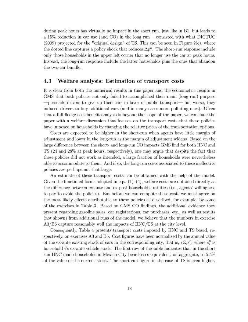
4.3 Welfare analysis: Estimation of transport costs

It is clear from both the numerical results in this paper and the econometric results in

GMS that both policies not only failed to accomplished their main (long-run) purpose

–persuade drivers to give up their cars in favor of public transport– but worse, they

induced drivers to buy additional cars (and in many cases more polluting ones). Given

that a full-fledge cost-benefit analysis is beyond the scope of the paper, we conclude the

paper with a welfare discussion that focuses on the transport costs that these policies

have imposed on households by changing the relative prices of the transportation options.

Costs are expected to be higher in the short-run when agents have little margin of

adjustment and lower in the long-run as the margin of adjustment widens. Based on the

large difference between the short- and long-run CO impacts GMS find for both HNC and

TS (24 and 28% at peak hours, respectively), one may argue that despite the fact that

these policies did not work as intended, a large fraction of households were nevertheless

able to accommodate to them. And if so, the long-run costs associated to these ineffective

policies are perhaps not that large.

An estimate of these transport costs can be obtained with the help of the model.

Given the functional forms adopted in eqs. (1)—(4), welfare costs are obtained directly as

the difference between ex-ante and ex-post household’s utilities (i.e., agents’ willingness

to pay to avoid the policies). But before we can compute these costs we must agree on

the most likely effects attributable to these policies as described, for example, by some

of the exercises in Table 3. Based on GMS CO findings, the additional evidence they

present regarding gasoline sales, car registrations, car purchases, etc., as well as results

(not shown) from additional runs of the model, we believe that the numbers in exercise

A3/B5 capture reasonably well the impacts of HNC/TS at the city level.

Consequently, Table 4 presents transport costs imposed by HNC and TS based, re-

spectively, on exercises A3 and B5. Cost figures have been normalized by the annual value

of the ex-ante existing stock of cars in the corresponding city, that is, Σ0 , where

0 is

household ’s ex-ante vehicle stock. The first row of the table indicates that in the short

run HNC made households in Mexico-City bear losses equivalent, on aggregate, to 5.5%

of the value of the current stock. The short-run figure in the case of TS is even higher,

18

9%, which would amount, in annual terms, to $120 million (in 2007 U.S. dollars).41

*** Insert Table 4 here or below ***

We cannot immediately read from the first row in Table 4 that TS was 1.6 times

costlier than HNC in the short-run because stock values, relative to total surplus, are

not the same. One possible correction is to normalize the ex-ante total surplus in each

economy to the same number (by simply adjusting the gross utility ), which is the

same as to normalize losses in TS by the stock value in Mexico-City. The second row

of the table shows that with this correction TS becomes 2.6 times costlier. The next

two rows in the table show that this cost difference extends to the long run; but more

importantly, that the long-run losses are surprisingly close to the short-run ones. One

possible explanation is that only a few households accommodated to the shocks after all.

This seems to be the case in both policies. In fact, the model indicates that only 6.2% of

the households that owned a single car before HNC decided to buy a second one and that

only 2.8% of all households in Santiago decided to buy a car (or an extra one) because

of TS.

But this is not the full story. Even if a policy prompts a much larger response in

terms of additional cars on the street, the long-run losses are still likely to be slightly

smaller than the short-run losses. As we increase the policy shock, not only we increase

the number of households adjusting to the shock but also the costs borne by those

that do not adjust.42 Overall, these numbers indicate that the long-run flexibility does

not provide much of a cost alleviation. Consequently, any cost-benefit analysis may well

abstract from long-run adjustment considerations. Large part of the reason for this latter

is that households that decided to buy an additional (or first) car because of the policy

were households that before the policy were not that far from buying that additional

(or first) car anyway; they didn’t do it before only because buying a car is a lumpy

investment.

41This number, which may be even slightly higher since was kept constant in the analysis despite

some increase in congestion, is the product of three variables: = 1404 (see below), Σ0 = 0945 million

(from INE) and 9.02% (from the model). was constructed as follows: the average vehicle in the city

of Santiago in 2006/2007 was US$6556 in value (from www.sii.cl) and 10.4 years old (from ANAC, see

fn. 79). And following conversations with ANAC, we then assumed an annual depreciation for such

car of $983 (15%) that divided by 0.7, to account for a 30% additional spending in insurance, taxes,

registration and some maintenance, leads to the number above (a similar number is obtained using a

2006 household survey). Unfortunately, we cannot carry out a similar exercise for HNC because of lack

of comparable information for 1989. If we use the numbers reported in Davis (2008, p. 78), which are

based on a 2005 household survey, we obtain a short run cost for HNC of $132 million annually (in 2006

U.S. dollars); figure that may be seen as an upper bound since the average value of a car running in

1989 was clearly lower than one in 2005.42Take for instance exercise B1 in Table 3. The long-run response is quite large, a 18,4% increase in

the stock; yet the difference between short- and long-run losses is again small: 27.6 vs 26.1%. Note that

this small difference also extends to "good" policies. For example, the short-run (transport) gains in B8

amount to 13.2% while the long-run gains to 13.6%.

19

Given the heterogeneous CO responses reported by GMS and supported by the numer-

ical results of our model, it is unlikely that the transport costs in Table 4 are distributed

evenly among households of varying incomes. We again use the model to shed some light

on this. Table 5 reports welfare costs for three groups of households: high-income (as

portrayed by exercises A4 and B6 in Table 3), middle-income or city-average (numbers

are in Table 4), and low-income (as portrayed by exercises A5 and B7). Not surprisingly,

middle-income households suffer the most in HNC; many of them own a single car but

only a few can afford a second one to by-pass the driving restriction. TS, on the other

hand, appears fairly regressive with low-income households being hit, on average, 3.5

times as bad as high-income ones.

*** Insert Table 5 here or below ***

5 Concluding remarks

We have developed a theoretical "bundling" model that characterizes the short and long-

run impacts of different transportation policies and for different income groups. The

model captures in a simple way the essential elements of a household’s decision problem

which are the allocation of existing vehicle capacity, if any, to competing uses (peak vs

off-peak hours) and how that capacity is adjusted in response to a policy shock. The

model was then applied to two major transportation policies —HNC in Mexico-City and

TS in Santiago— to illustrate precisely how it can be of great complement in empirical

analysis.

We learned from HNC that driving restriction policies can be effective in reducing

congestion and pollution but only in the short-run. As these policies appear politically

feasible –they have been applied in quite a few cities in Latin America (see Table 1) and

elsewhere (e.g., Beijing, Tianjin)– and are relatively easy to enforce, there is more to

be understood on how to design them as to reap the short-run gains without prompting

the long-run losses associated to the purchase of additional (higher-emitting) vehicles;

perhaps some combination of a permanent ban on older vehicles and a sporadic one on

newer vehicles to attack a limited number of episodes/days of bad pollution (the model

shows that a permanent ban can also work as intended as far as older, higher polluting

vehicles are under strict control, i.e., prohibition of their import into the city and gradual

retirement of existing ones).

The TS experience, on the other hand, showed how rapidly commuters can abandon

public transport in favor of cars after a (permanent) deterioration in the quality of service.

But even more successful public transport reforms (e.g., Transmilenio in Bogotá) indicate

that it is challenging to persuade drivers to give up their cars. We believe there is a lot

more to learn on how commuters decide between public and private transportation and

the role different instruments –including road pricing and pollution/gasoline taxes–

play in that decision. This is particularly important in cities that exhibit a fast increasing

20

motorization rate, not only for dealing with local problems such as urban air pollution

and congestion, but also, with the global problem of carbon emissions

References

[1] Armstrong, M. and J. Vickers (2010), Competitive nonlinear pricing and bundling,

Review of Economic Studies 77, 30-60.

[2] Beaton, S., G. Bishop, D. Stedman (1992), Emission characteristics of Mexico City

vehicles, Journal of Air and Waste Management 42, 1424-1429.

[3] Briones, I. (2009), Transantiago: Un problema de informacion, Estudios Publicos

16, 37-91.

[4] Caffera, M. (2011), The use of economic instruments for pollution control in Latin

America: Lessons for future policy design, Environment and Development Eco-

nomics 16, 247-273.

[5] Cantillo, V., and J.D. Ortuzar (2011), Restricting cars by license plate numbers: An

erroneous policy for dealing with transport externalities, mimeo, Universidad del

Norte, Colombia.

[6] CONAMA (2004), Plan de Prevención y Descontaminación Atmosférica de la Región

Metropolitana, CONAMA Metropolitana de Santiago, Chile.

[7] Davis, L. (2008), The effect of driving restrictons on air quality in Mexico City,

Journal of Political Economy 116, 38-81.

[8] DICTUC (2009), Evaluación Ambiental del Transantiago, Report prepared for the

United Nations Environment Programmme, DICTUC, Santiago.

[9] Eberly, J. (1994), Adjustment of consumers’ durables stocks: Evidence from auto-

mobile purchases, Journal of Political Economy 102, 403-436.

[10] EIU (2010), Latin America Green City Index: Assesing the Environmental Perfor-

mance of Latin America’s Major Cities, Economist Intelligence Unit (EIU), Munich.

[11] Eskeland, G., and T. Feyzioglu (1997), Rationing can backfire: The "day without a

car" in Mexico City, World Bank Economic Review 11, 383-408.

[12] Gallego, F., J.-P. Montero, and C. Salas (2013), The effect of transport policies on

car use: Evidence from Latin American cities, working paper, PUC-Chile.

[13] GDF (2004), Actualización del Programa Hoy No Circula, Report, Gobierno del

Distrito Federal (GDF), Mexico, June.

21

[14] Ide, E. and P. Lizana (2011), Transportation policies in Latin America, working

paper, PUC-Chile.

[15] INEGI (1989), La Industria Automotriz en México, Instituto Nacional de Estadística

Geográfica e Informática (INEGI), México.

[16] Litman, T. (2011), Transit price elasticities and cross-elasticities, Discussion paper,

Victoria Transport Policy Institute (originally published in the Journal of Public

Transportation 7 (2004), 35-58).

[17] Molina, L., and M. Molina (2002), Eds., Air Quality in the Mexico Megacity: An

Integrated Assessment, Kluwer Academic Publishers, Dordrecht.

[18] Muñoz, J.C., J.D. Ortuzar, and A. Gschwender (2009), Transantiago: The fall and

rise of a radical public transport intervention, In: W. Saleh and G. Sammer (Eds.),

Travel Demand Management and Road User Pricing: Success, Failure and Feasibil-

ity, Ashgate, Farnham, pp. 151-172.

[19] Onursal, B. and S.P. Gautam (1997), Vehicular air pollution: Experiences from seven

Latin American urban centers, World Bank Technical Paper No. 373, Washington,

DC.

[20] Robertson, S., H. Ward, G. Marsden, U. Sandberg, and U. Hammerstrom (1998),

The effects of speed on noise, vibration and emissions from vehicles, working paper,

UCL.

[21] SDG (2005), Estudio de Tarificación Vial para la Ciudad de Santiago, Report

prepared for the United Nations Development Programmme, Steer-Davies-Gleave

(SDG), Santiago.

[22] Small, K. and E. Verhoef (2007), The Economics of Urban Transportation, Rout-

ledge, New York.

22

Appe

     Sou

 

   Sourc

endix A: M

rce: GMS 

ce: GMS 

unicipalityy results inn GMS 

 

 

Appendix B: Option value

Suppose there is a probability 1 that the enacted policy (e.g., HNC, TS) is cancel

in the future, say at time . The relevant discount factor is 1. The cost of car is

and the lemon cost is , so the resale price of the car is (1− ). A household has four

investment options: (i) invest in the car today and sell it at if the authority decides to

cancel the policy, (ii) wait until and buy the car only if the authority decides to keep

the policy in place, (iii) never invest in a car, and (iv) invest in the car today and keep

it at regardless of whether the authority decides to cancel the policy or not.

Because of the irreversibility and uncertainty there is an option value of waiting (or

an additional cost if the car is bought today). This is only relevant for those that are

indifferent between options (i) and (ii). Households that go for (iii) are far from buying

the car anyway, so the policy doesn’t affect them at all. Households that go for (iv)

are those for who the policy is sufficiently important that are willing to kill the option

anyway (there may be none if is big enough).

Let ∆ the utility gain from buying a car. The expected (additional) utility from

following option (i) is

[∆ ] = ∆− + {[(1− ) −∆] + (1− )× 0}

One may be tempted to conclude that all houselholds for which [∆ ] ≥ 0, or ∆ is

equal or greater than the cutoff

c∆ =

µ1 +

1−

¶

should buy the car. This is not correct because we need to add the cost of "killing" the

option of waiting. To do this, we need to compute the expected additional utility from

following option (ii):

[∆ ] = 0 + {× 0 + (1− )(∆− )}

The utility cutoff that makes [∆ ] = [∆ ] is

c∆ =

µ1 +

1−

¶ c∆

so the difference c∆ − c∆ = 2(1− )

(1− )(1− )

is the cost of killing the option. This cost is increasing in and decreasing or increasing

in depending on whether1

≶ 1 +

√1−

24

More importantly, a household follow (i) only if

∆ ≥ c∆

This result can be easily taken to the analysis in Figure 2. For example, take the indiffer-

ent household in Figure 2(a) (the case of a a TS-like policy captured by a shift of relative

prices from ∆2 to ∆2 + ). For some households to go for investment option (i)

we require now

≥

1− 0

Note that when = 0, there will be always some households buying the car even if

is very small. However as increases the policy intervention must be big enough. Note

that if = 0, the parameter becomes irrelevant since there is never the option to think

about returning the car, i.e., we go back to basic analysis that in the main text.

25

Table 1. Transport policies in Latin America

Program City Start year Type Scope

Restricción Vehicular Santiago 1986 DR gradual

Hoy No Circula Mexico D.F. 1989 DR drastic

Metrobus-Q Quito 1995 PT gradual

Operação Rodizio Sao Paulo 1996 DR gradual

Pico y Placa Bogotá 1998 DR gradual

Transmilenio Bogotá 2000 PT gradual

Pico y Placa Medellín 2005 DR drastic

Metrobus México D.F. 2005 PT gradual

Restricción Vehicular San José 2005 DR gradual

TranSantiago Santiago 2007 PT drastic

Pico y Placa Quito Quito 2010 DR drasticDR: driving restriction; PT: public transportation reform.The program suffered a temporary interruption in June-July of 2009.

Source: Ide and Lizana (2011)

Table 2. CalibrationTargets HNC TS Parameters HNC TS

= 0 0.71 0.62 ∆ 0.91 0.91

= 1 0.23 0.30 ∆ 1.01 1.23

= 2 0.06 0.08 0.95 1.22

0.16 0.31 0.90 1.20

0.16 0.32 0.29 0.40

0.98 0.85 0.98 0.95

1

Table 3. SimulationsExercise ∆

∆ ∆

∆ ∆ stock

Panel A: HNC

A1 -12.5% -12.1% -8.3% -8.1% -9.2%

A2 -12.5% -12.1% -2.7% -2.0% 4.1%

A3 -12.5% -12.1% 11.0% 12.1% 4.1%

A4 -1.7% -1.7% 3.9% 4.2% 3.0%

A5 -20.4% -20.6% 2.3% 3.0% 2.6%

Panel B: TS

B1 0.0% 0.3% 27.8% 28.1% 18.4%

B2 4.5% -4.4% 28.2% -0.1% 11.5%

B3 0.0% 0.0% 8.1% 8.1% 5.3%

B4 0.4% -0.3% 11.2% 5.7% 5.4%

B5 0.4% -0.3% 27.5% 7.1% 5.4%

B6 2.0% 0.0% 18.6% 0.3% 1.6%

B7 0.4% -0.3% 41.5% 10.1% 9.4%

B8 -0.6% 0.4% -15.2% -8.5% -7.9%

Table 4. Transport costs inflicted by HNC and TS

Costs HNC TS ratio TS/HNC

Short-run 5.47% 9.02% 1.6

Short-run (corrected) 5.47% 14.30% 2.6

Long-run 5.29% 8.84% 1.6

Long-run (corrected) 5.29% 14.03% 2.7

Long-run ( = 0) 4.71% 14.03% 3.0

Table 5. Transport costs as a function of income

Income group HNC (SR) HNC (LR) TS (SR) TS (LR)

Low 2.29% 2.25% 11.39% 11.30%

Middle 5.47% 5.29% 9.02% 8.84%

High 3.27% 2.73% 3.38% 3.25%

2

1

Figure 1. Decision to own a vehicle based on vertical preferences

hq

lq

hp

rk

0

1

group A

group B

lp

rk

group C

group D

k

k

1

prkqq lh /

group D

group E

bus for h and l

bus for h1 car for l

1 car for hbus for l

hh

hh q

tp

x22

1ˆ

1 car for h and l

ll

ll

l

xt

rq

t

p ~222

1

ll

ll q

t

px

22

1ˆ

Figure 2(a). Households in group A

hx

lx hh

hh

h

xt

rq

t

p ~222

1

0 1

1

h1

h2

h3

2

bus for h and l

bus for h1 car for l

1 car for hbus for l

hh

h

kt

p

22

1

1 car for h and ll

ll

l

t

rk

t

p

222

1

ll

l

kt

p

22

1

Figure 2(b). Households in group B

hx

lxh

hh

h

t

rk

t

p

222

1

0 1

1

l1

l2

lh33 ,

h1

h2

bus for h and l

bus for h1 car for l

1 car for hbus for l

hh

llhh

t

r

t

kqpqp

22

)(

2

1

2 cars for h and l

ll

l

t

rk

t

p

222

1

l

llhh

l

t

qpkqp

t

r

2

)(

22

1

Figure 2(c). Households in group C1

hx

lxhh

h

t

rk

t

p

222

1

0 1

1

h1

l1

h2

l2

3

bus for h and l

bus for h1 car for l

2 cars for hbus for l

hh

llhh

t

r

t

kqpqp

22

)(

2

1

2 cars for h and l

ll

l

t

rk

t

p

222

1

ll

l

qt

p

22

1

Figure 2(d). Households in group D1

hx

lxh

hh

h

t

rq

t

p

222

1

0 1

1

h

l

bus for h and l

bus for h2 cars for l

2 cars for hbus for l

hh

h

qt

p

22

1

2 cars for h and ll

ll

l

t

rq

t

p

22

1

ll

l

qt

p

22

1

Figure 2(e). Households in group E

hx

lxh

hh

h

t

rq

t

p

22

1

0 1

1