Course Title: Distributed Database Management Systems ... to 45 lectures.pdf · C50001 Suhail...

1

Course Title: Distributed Database Management Systems

Course Code: CS712

Instructor: Dr. Nayyer Masood ([email protected])

Lecture No: 23& 24

In previous lecture:

- Fragmentation

In this lecture:

- Reasons for Fragmentation

o Maximizes local access

o Reduces table size, etc.

- PHF using the SQL Server on same machine

- Implemented PHF in a Banking Environment

Fragmentation

• We know there are different types, we start with the simplest one and that is the PHF

• Supposedly, you have already gone through the design phase and have got the predicates to be used as

basis for PHF, just as a reminder

• From the user queries, we first collect the simple predicates and then we form a complete and minimal

set of minterm predicates, a minterm predicate is ….., you know that otherwise refer back to lecture 16,

17

• Lets say we go back to our Bank example, and lets say we have decided to place our servers at QTA and

PESH so we have two servers where we are going to place our PHFs

2

• As before we register our servers and now at our Enterprise Manager we can see two instances of SS

• At each of the three sites we define one database named BANK and also one relation, normal base table,

however, for the fragmentations to be disjoint (a correctness requirement) we place a check on each

table at three sites, how….

• We name our fragments/local tables as custQTA, custPESH

• Each table is defined as

create table custPESH(custId char(6), custName varchar(25), custBal number(10,2), custArea char(5))

• In the same way we create 2 tables one at each of our two sites, meant for containing the local users

• Users that fall in that area and the value of the attribute custArea is going to be the area where a

customer’s branch is, so its domain is {pesh, qta)

• To ensure the disjointness and also to ensure the proper functioning of the system, we apply a check on

the tables

• The check is

• Peshawar customers are allocated from the range C00001 to C50000, likewise

• QTA is C50001 to C99999

• So we apply the check on both tables/fragments accordingly, although they can be applied while

creating the table, we can also apply them later, like

• Alter table custPesh add constraint chkPsh check ((custId between ‘C00001’ and ‘C50000’) and

(custArea = ‘Pesh’))

• Alter table custQTA add constraint chkQta check ((custId between ‘C50001’ and ‘C99999’) and

(custArea = ‘Qta’))

• Tables have been created on local sites and are ready to be populated, start running applications on

them, and data enters the table, and the checks ensure the entry of proper data in each table. Now, the

tables are being populated

Example Data in PESH

C0001 Gul Khan 4593.33 Pesh

C0002 Ali Khan 45322.1 Pesh

C0003 Gul Bibi 6544.54 Pesh

C0005 Jan Khan 9849.44 Pesh

Example Data at QTA

C50001 Suhail Gujjar 3593.33 Qta

C50002 Kauser Perveen 3322.1 Qta

C50003 Arif Jat 16544.5 Qta

C50004 Amjad Gul 8889.44 Qta

3

• Next thing is to create a global view for the global access/queries, for this we have to link the servers

with each other, this is required

• You have already registered both the servers, now to link them

• You can link them using Enterprise Manager or alternatively through SQL, we do here using SQL

Connect Pesh using Query Analyzer

• Then execute the stored procedure sp_addlinkedserver

• The syntax is

•

sp_addlinkedserver

@server = ‘QTA',

@srvproduct = '',

@provider = 'sqloledb', @datasrc = ‘mysystem\QTA‘

• You will get two messages, if successful, like ‘1 row added’ and ‘1 row added’

• You have introduced QTA as a linked server with PESH.

• We have to perform this operation on the other server, that is, we have to add linked server PESH at

QTA

• Setup is there, next thing is to create a partitioned view

• In SQL Server, a partitioned view joins horizontally partitioned data across multiple servers

• The statement to create the partitioned view is

Create view custG as select * from custPesh

Union All

select * from QTA.bank.dbo.custQTA

• Likewise, we have to apply same command at QTA

• Create view custG as

select * from custQta

Union All

select * from PESH.bank.dbo.custPesh

• Once it is defined, now when you access data from custG, it gives you data from all four sites.

• It is also transparent

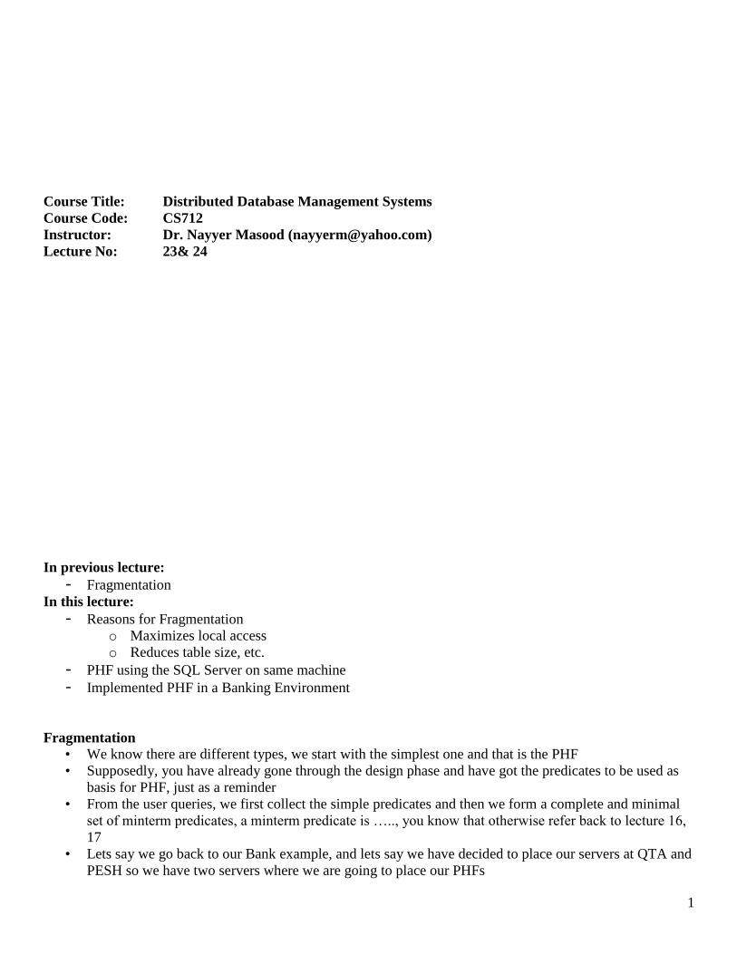
• Now lets say if you are connected with Pesh, and you give the command

Select * from custPesh

You get the output

4

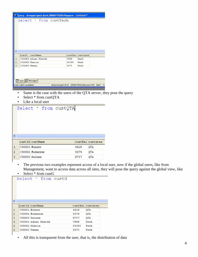
• Same is the case with the users of the QTA server, they pose the query

• Select * from custQTA

• Like a local user

• The previous two examples represent access of a local user, now if the global users, like from

Management, want to access data across all sites, they will pose the query against the global view, like

• Select * from custG

• All this is transparent from the user, that is, the distribution of data

5

• Global user gets the feeling, as if all the users’ data is placed on a single place

• For the administrative purposes they can perform analytical types of queries on this global view, like

Summary:

We have discussed the fragmentation, maximize local access and reduce table size etc. and also discussed the

PHF using the SQL Server on same machine.


Course Code: CS712


Lecture No: 25


- Reasons for Fragmentation

o Maximizes local access

o Reduces table size, etc.

- PHF using the SQL Server on same machine

- Implemented PHF in a Banking Environment

- DDBS layer is superimposed on the client sites

- Actual Data resides with the local sites

In this lecture:

- Derived Horizontal Fragmentation

Derived Horizontal Fragmentation

6

• Fragmenting/ partitioning a table based on the constraints defined on another table.

• Both tables are linked with each other through Owner-Member relation

Scenario

Why DHF Here

• Employee and salary record is split in two tables due to Normalization

• Storing all data in EMP table introduces Transitive Dependency

• That causes Anomalies

PHF of TITLE table

a, b, c,

d

p, q, r, s,

a

TABLE

1

TABLE

2

Link

Owner

Member

empId, empName, empAdres, titleId

titleId, titleName,

sal

EMP

TITLE

Link

Owner

Member

7

• Predicates defined on the sal attribute of TITLE table

• p1 = sal > 10000 and sal <= 20000

• p2 = sal > 20000 and sal <= 50000

• p3 = sal > 50000

Conditions for the TITLE Table

• TITLE1 = (sal > 10000 and SAL ≤30000) (SAL)

• TITLE2 = (sal > 20000 and SAL ≤50000) (SAL)

• TITLE3 = (sal > 50000) (SAL)

Tables created with constraints

• create table TITLE1 (titleID char(3) primary key, titleName char (15), sal int check (SAL between

10000 and 20000))

• create table TITLE2 (titleID char(3) primary key, titleName char (15), sal int check (SAL between

20001 and 50000))

• create table TITLE3 (titleID char(3) primary key, titleName char (15), sal int check (SAL > 50000))

TITLE

titleID titleName Sal

T01 Elect. Eng 42000

T02 Sys Analyst 64000

T03 Mech. Eng 27000

T04 Programmer 19000

TITLE1



TITLE3



TITLE2



T03 Mech. Eng 27000

EMP table at local sites

create table EMP1 (empId char(5) primary key, empName char(25), empAdres char (30), titleId char(3)

foreign key references TITLE1(titleID))

8

Referential Integrity Constraint

• Null value in the EMP1.titleId is allowed

• This violates the correctness requirement of the Fragmentation, i.e., it will violating the completeness

criterion

Tighten Up the Constraint Around

• Further we need to impose the “NOT NULL” constraint on the EMP1.titleID

• Now the records in EMP1 will strictly adhere to the DHF

Revised EMP1 Definition

create table EMP1 (empId char(5) primary key, empName char(25), empAdres char (30), titleId char(3)

foreign key references TITLE1(titleID) not NULL)

Defining all three EMP

• create table EMP1 (empId char(5) primary key, empName char(25), empAdres char (30), titleId char(3)






PHF of EMP at different sites

• create table EMP1 (empId char(5) primary key check (empId in ('Programmer')), empName char(25),

empAdres char (30), titleId char(3))

empId, empName, empAdres, titleId

titleId, titleName, sal

EMP

TITLE

Link

PHF on Owner

Member Natural Join with Owner Fragments

9

• create table EMP2 (empId char(5) primary key check (empId in (‘Elect. Engr’,’Mech. Engr’)),

empName char(25), empAdres char (30), titleId char(3))

• create table EMP3 (empId char(5) primary key check (empId in (' Sys Analyst ')), empName char(25),

empAdres char (30), titleId char(3))

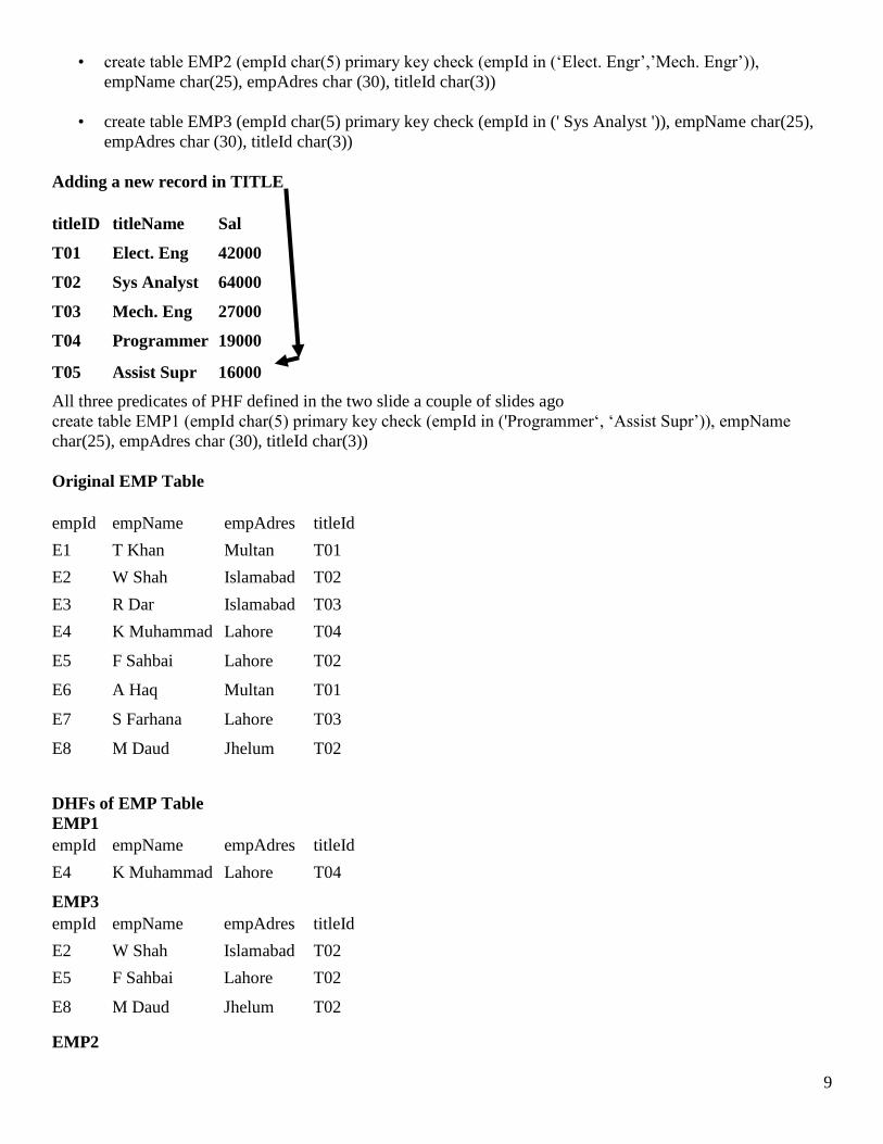
Adding a new record in TITLE




T03 Mech. Eng 27000


T05 Assist Supr 16000

All three predicates of PHF defined in the two slide a couple of slides ago

create table EMP1 (empId char(5) primary key check (empId in ('Programmer‘, ‘Assist Supr’)), empName

char(25), empAdres char (30), titleId char(3))

Original EMP Table

empId empName empAdres titleId

E1 T Khan Multan T01

E2 W Shah Islamabad T02

E3 R Dar Islamabad T03

E4 K Muhammad Lahore T04

E5 F Sahbai Lahore T02

E6 A Haq Multan T01

E7 S Farhana Lahore T03

E8 M Daud Jhelum T02

DHFs of EMP Table

EMP1


E4 K Muhammad Lahore T04

EMP3


E2 W Shah Islamabad T02

E5 F Sahbai Lahore T02

E8 M Daud Jhelum T02

EMP2

10


E1 T Khan Multan T01

E3 R Dar Islamabad T03

E6 A Haq Multan T01

E7 S Farhana Lahore T03

Transactional Replication

• Data replicated as the transaction executes

• Preferred in higher bandwidth and lower latency

• Transaction is replicated as it is executed

• Begins with a snapshot, changes sent at subscribers as they occur or at timed intervals

• A special Type allows changes at subscribers

From the Enterprise Manager, select Replication, after a couple of nexts, we get this screen

12

Publication has been created that can be viewed from Replication Monitor or from Replication, like this

It has also created snapshot and log reader agents, which won’t work until we create a subscription. For this, we

select the publication from replication monitor, right click it, and then select Push new subscription.

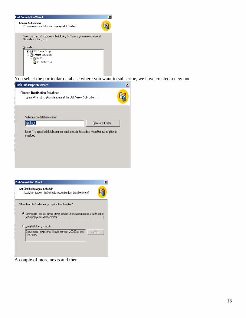
13

You select the particular database where you want to subscribe, we have created a new one.

A couple of more nexts and then

14

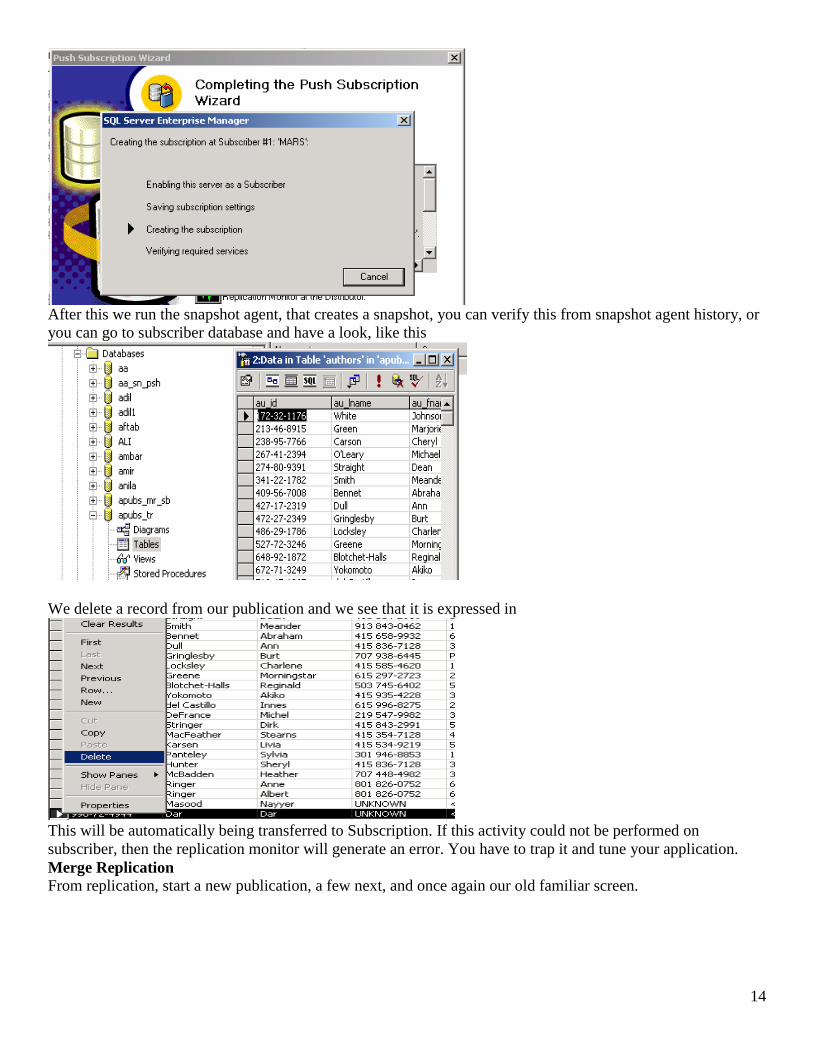
After this we run the snapshot agent, that creates a snapshot, you can verify this from snapshot agent history, or

you can go to subscriber database and have a look, like this

We delete a record from our publication and we see that it is expressed in

This will be automatically being transferred to Subscription. If this activity could not be performed on

subscriber, then the replication monitor will generate an error. You have to trap it and tune your application.

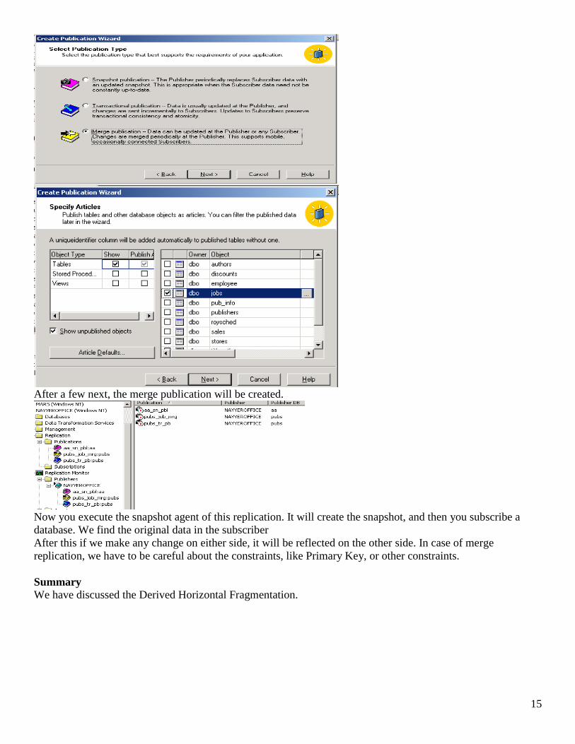
Merge Replication

From replication, start a new publication, a few next, and once again our old familiar screen.

15

After a few next, the merge publication will be created.

Now you execute the snapshot agent of this replication. It will create the snapshot, and then you subscribe a

database. We find the original data in the subscriber

After this if we make any change on either side, it will be reflected on the other side. In case of merge

replication, we have to be careful about the constraints, like Primary Key, or other constraints.

Summary

We have discussed the Derived Horizontal Fragmentation.

16


Course Code: CS712


Lecture No: 26

In this lecture:

- Transaction Management

o Basics

o Properties of Transaction

Database and Transaction Consistency

The concept of transaction is used within the database domain as a logical unit of work. A database is in a

consistent state if it obeys all of the consistency (integrity) constraints defined over it state changes occur due to

modifications, insertions and deletions (together called updates). The database can be temporarily inconsistent

during the execution of a transaction. The important point is that the database should be consistent when then

transaction terminates as shown in figure 1

17

Figure 1: A Transaction Model

Transaction consistency refers to the actions of concurrent transactions. Transaction Management is difficult in

case of the concurrent access to the database by multiple users. Multiple read-only transactions cause no

problem at all, however, if one or more of concurrent transactions try to update data that may cause problem. A

transaction is considered to be a sequence of read or/and write operations; it may even consist of a single

statement.

Transaction Example T-SQL

Transaction BUDGET_UPDATE

begin

EXEC SQL UPDATE J

SET BUDGET = BUDGET * 1.1

WHERE JNAME = “CAD/CAM"

end

The Begin_transaction and end statements delimit a transaction. The use of delimiters is not enforced in every

DBMS.

Example Database

Airline Reservation System

– FLIGHT(fNo, fDate, fSrc, fDest, stSold, fCap)

– CUST(cName, cAddr, cBal)

– FC(fNo, fDate, cName, cSpecial)

Let us consider a simplified version of a typical reservation application, where a travel agent enters the flight

number, the date, and a customer name and asks for a reservation. The transaction to perform this function can

be implemented as follows, where database accesses are specified in embedded SQL notation:

Begin_transaction Reservation

input(flight_no, dt, c_name);

EXEC SQL Select stSold, cap into temp1, temp2

where fNo = flight_no and date = dt

Begin Transaction T

Consistent State of DB

May be Temporarily Inconsistent

Consistent State

Execution of Transaction T

End of Transaction T

18

if temp1 = temp2 then

output("no free seats"); Abort

else

EXEC SQL update flight

set stSold = stSold + 1 where

fNo = flight_no and date = dt;

EXEC SQL insert into FC values (flight_no,

dt, c_Name, null); Commit;

output("reservation completed")

end

The transaction on

Line 1: is to input the flight number, the date and the customer name.

Line 2: updates the number of sold seats on the requested flight by one.

Line 3: inserts a tuple into the FC relation here we assume that customer is old one so its not necessary to have

an insertion into the CUST relation.

Line 4: reports the result of the transaction to the agent’s terminal.

Termination conditions of Transaction

If transaction can complete its task successfully, we say that the transaction commits. If a transaction stops

without completing its tasks, we say that it aborts when a transaction is aborted its execution is stopped and all

of its already executed actions are undone by returning the database to the state before their execution. This is

also known as rollback.

Characterization of Transaction

Read and Write are major operations of database concern in a transaction.

Read set (RS): The set of data items that are read by a transaction.

Write set (WS): The set of data items whose values are changed by this transaction

The read set and write set of a transaction need not be mutually exclusive. Finally, the unions of the read set and

write set of a transaction constitutes its base set

(BS = RS U WS)

Formalization of the Transaction Concept

Let Oij(x) be some operation Oj of transaction Ti operating on data item x, where Oj € {read,write} and Oj is

atomic. Let OSi denote the set of all operations in Transaction Ti, OSi = Uj Oij. We denote by Ni the

termination condition for Ti, where Ni € {abort,commit}.

Transaction Ti is a partial order Ti = {∑i, <i} where

1- ∑i = OSi U {Ni }

2- For any two operations Oij, Oik € OSi , if Oij = R(x) and Oik = W(x) for any data item x, then either

OijiOik or Oik <i Oij.

3- V Oij € OSi, Oij <i Ni

The first condition specify the domain as the set of read and write operation that make up the transaction, plus

the termination condition, which may be commit or abort. The second condition specifies the ordering relation

between the conflicting read and write operations of the transaction, while the final condition indicates that the

termination condition always follows all other operations.

There are two points about this definition

First the ordering relation < is given and the definition does not attempt to construct it.

Second, condition two indices that the ordering between conflicting operations has to exist within <.

19

Conflicting Operations

Two operations Oi(x) and Oj(x) are said to be in conflict, Oi = write or Oj = write (at least one of them is write

and they access the same data item).

Example

Consider a transaction T that consists following steps:

Read(x)

Read(y)

x = x + y

Write(x)

Commit

ACID Properties of a Transaction

The consistency and reliability aspects of transactions are due to our properties:

1- Atomicity: also known as “all or none” property

– refers to the atomicity of entire Tr rather than an individual operation

– It requires from system to define some action in case of any interruption in execution of Tr.

– Two types of failures requiring procedures from Transaction Recovery or Crash Recovery

2- Consistency: refers simply to the correctness of a transaction

– A Tr should transform the DB from one consistent state to another consistent state.

– Concern of Semantic Integrity Control and Concurrency Control

– Classification of consistency for Trs uses the term “Dirty Data”; data that has been updated by a

Tr before its commitment.

Degree 3: Transaction T sees degree 3 Consistency if:

1- T does not overwrite dirty data of other transactions

2- T does not commit any writes until it completes all its writes (i.e., until end of transaction)

3- T does not read dirty data from other transactions

4- Other transactions do not dirty any data read by T before T completes




3- T does not read dirty data from other transactions






3- Isolation

- A transaction cannot reveal its results to other transactions before commitment

- Required in particular when one of the transactions is updating a common data item

Example

20

Consider two concurrent transactions T1 and T2 both access data item x. assume that the value of x before they

start executing is 50.

- T1: Read(X) T2: Read(x)

x = x+1 x = x+1

Write(x) Write(x)

Commit Commit

Two possible serial executions are T1, T2 or T2, T1. First transaction gets 50 and makes it 51, other makes it

52. In any case it will be 52 at the end of both transactions. An interleaved execution may result “Lost Update”.

Like

(T1:Read(x), T1:x =x+1,

T2:Read(x), T1:Write(x),

T2:x=x+1, T2:write(x),

T1:commit, T2:commit)

Summary

We have discussed the transaction management, its basics and the properties of transaction (ACID).


Course Code: CS712


Lecture No: 27

21


- Defined Transaction Formally

- ACID Properties of a Transaction

In this lecture:

- ACID Properties

- Types of Transaction

- Transaction in DDBS

ACID Properties

3- Isolation

Isolation and consistency are interrelated, one supports other. Degree 3 provides full isolation. SQL-92

identified isolation levels based on following phenomena.

Dirty Read: A transaction reads the written value of another transaction before its commitment, like,

--, W1(x), ----, R2(x), --- ,C1(or A1)-----, C2(or A2).

Non-repeatable or Fuzzy Read: Two reads of same data item by same transaction and a write by another

transaction on the same data item

--, R1(x), ----, W2(x), --- ,C2-----, R1(x)----

Phantom: T1 performs a read on a predicate, T2 inserts tuples that satisfy the predicate

--, R1(P), ----, W2(yinP), --- ,C2(orA2)-----, C1(orA1)---

Isolation levels

• Read Uncommitted: all three phenomena possible

• Read Committed: fuzzy read, phantoms possible; DR not possible

• Repeatable Read: Only phantoms possible

• Anomaly Serializable: None of the phenomena possible

4- Durability:

Durability refers to that property of transaction which ensures that once a transaction commits, its results are

permanent and can not be erased from the database.

Types of Transactions

Transactions have been classified according to a number of criteria one criterion is the duration of transaction.

Transaction may be classified as

• on-line (short-life)

• batch (long-life)

Online transactions are characterized by very short execution/response times and by access to a relatively small

portion of the database. Examples are banking and airline reservation transactions.

Batch transactions are CAD/CAM databases, statistical applications, report generation, complex queries and

image processing.

Another classification is with respect to the organization of the read write actions if the transactions are

restricted so that all the read actions are performed before any write action, the transaction is called a two-step

transaction.

If transaction is restricted so that a data item has to be read before it can be updated (written), the corresponding

class is called restricted (or read-before-write).

If a transaction is both two-step and restricted, it is called a restricted two-step transaction.

22

Transactions can be classified according to their structure. Four broad categories

– flat (or simple) transactions

– closed nested transactions

– open nested transactions

– workflow models

1) Flat transaction

• Consists of a sequence of primitive operations embraced between a begin and end markers.

• Begin_transaction Reservation

• …

• end.

2) Nested transaction

• The operations of a transaction may themselves be transactions.

• Begin_transaction Reservation

…

Begin_transaction Airline

…

end {Airline}

end {Reservation}

• Have the same properties as their parents; may themselves have other nested transactions.

• Introduces concurrency control and recovery concepts within the transaction.

Closed nesting

• Sub transactions begin after their parents and finish before them

• Commitment of a sub transaction is conditional upon the commitment of the parent (commitment

through the root)

Open nesting

• Sub transactions can execute and commit independently.

• Compensation may be necessary.

3) Workflows

• Flat transaction model suits relatively small and simple environments

• Certain environments need combination of open and nested models.

• A candidate definition “ a collection of tasks organized to accomplish some business activity”

• Different types of workflows.

• Workflows generally involve long transactions, like a reservation transaction that may include Airline,

Hotel, Auto reservations and bill generation.

• Workflows exhibit open nesting semantics

• So permits access to the results of sub-activity before the commitment of the major activity.

• Some components are declared as vital, main activity aborts if a vital component aborts, otherwise it

may commit even if a non-vital component aborts, like

• Compensating Transactions

• Contingency Transactions.

That concludes our basic discussion on Transactions.

Distributed Concurrency Control

Concurrency control concerns synchronizing concurrent transactions maintaining consistency of the database

and maximizing degree of concurrency.

23

Schedule or History

An order in which the operations of a set of transactions are executed. A schedule (history) can be defined as a

partial order over the operations of a set of transactions.

T1:

Read(x)

Write(x)

Commit

T2:

Write(x)

Write(y)

Read(z)

Commit

T3:

Read(x)

Read(y)

Read(z)

Commit

Complete Schedule

A complete schedule S over a set of transactions T={T1, …, Tn} is a partial order

• SCT(T, <T) where

• T = Ui i , for i = 1, 2, …, n

• <T U <i , for i = 1, 2, …, n

• For any two conflicting operations Oij, Okl € T, either Oij <T Okl or Okl <T Oij

T1:

Read(x)

Write(x)

Commit

T2:

Write(x)

Write(y)

Read(z)

Commit

T3:

Read(x)

Read(y)

Read(z)

Commit

1 = {R1(x), W1(x), C1}

2 = {W2(x), W2(y), R2(z), C2}

3 = {R3(x), R3(y), R3(z), C3}

= 1 U 2 U 3

= {R1(x), W1(x), C1, W2(x), W2(y), R2(z), C2, R3(x), R3(y), R3(z), C3}

A schedule is a prefix of a complete schedule such that only some of the operations and only some of the

ordering relationships are included.

Serial Schedule

If all the transactions included in it execute one after another. A serial schedules always leaves the database in a

consistent state. They may end up with a different final state of DB each one of them being consistent. If we

have three transactions, T1, T2, T3 then one serial schedule may be: T1 <S T3 <s T2 or T1 T3 T2

Interleaved Schedule

A schedule is in which operations from different transactions are mixed with each other in execution.

Like

S1 ={W2(x), R1(x), R3 (x), W1(x),C1, W2(y), R3(y), R2(z),C2 ,R3 (z), C3} is

an interleaved schedule.

Summary

We have discussed the ACID properties and the types of transaction. The types are flat transaction, nested

transaction and workflow. Also we have discussed the transaction in DDBS.

24


Course Code: CS712


Lecture No: 28


- Types of Transaction

- Transaction in DDBS

- Serial Transactions

- Conflicting Transactions

In this lecture:

- Serializability Theory

- Serializability Theory in DDBS

Equivalent Schedules

Two schedules S1, S2 defined over same T are equivalent if they have same effect on the database, that is, leave

database in same final state. Formally, if for each pair of conflicting operations

Oij and Okl (i ≠ k) if Oij <1 Okl then Oij <2 Okl

25

The phenomenon is also called conflict equivalence.

Serializable Schedule

If it is conflict equivalent to a serial schedule, i.e., the final state in which it leaves the database is equivalent to

a serial schedule-

• Ss ={W2(x), W2(y), R2(z), C2, R1(x), W1(x), C1, R3(x), R3(y), R3(z), C3}

• S1 = {W2(x), R1(x), R3 (x),W1(x),C1, W2(y), R3(y), R2(z),C2 ,R3(z), C3}

• Ss ={W2(x), W2(y), R2(z), C2, R1(x), W1(x), C1, R3(x), R3(y), R3(z), C3}

• S2 ={W2(x), R1(x), W1(x), C1, R3(x), W2(y), R3(y), R2(z), C2, R3(z), C3}

The function of the concurrency controller is to generate serializable schedule.

Fragmented Databases

The serializability is straight forward. Local transaction is independent of each other; each concerns local data.

In case of global transactions local sub transactions will be treated as different transactions.

Replicated Databases

T1:

Read(x)

x = x + 5

Write(x)

Commit

T2:

Read(x)

x = x*10

Write(x)

Commit

LS1={R1(x), W1(x),C1, R2(x), W2(x), C2}

LS2={R2(x), W2(x), C2, R1(x), W1(x), C1}

All values of replicated data should be same

1. Local Schedule same

2. Conflicting Ops in same relative order on all sites.

3. Logical and physical data items

4. User issues Ops on logical data items

5. Replica control maps to physical ones-

6. ROWA Protocol

7. Reduces availability in case of failure

8. Different algorithms, different replications.

Concurrency Control Algorithms • Different categorizations possible

• Like, mode of distribution, network topology-

• Synchronization primitive is the most common

• Locking and Ordering

• Pessimistic & Optimistic.

• Pessimistic approach synchronizes transactions early

• Optimistic do this late in execution life cycle of transactions

• Pessimistic

• Locking-based

• Centralized Locking

• Primary Copy Locking

26

• Distributed Locking-

• Timestamp Ordering (TO)

• Basic TO

• Multiversion TO

• Conservative TO

• Hybrid

• Optimistic

• Locking-based

• Timestamp ordering-based.

Locking based Concurrency Control

• Basic idea is that data items accessed by conflicting operations are accessed by one operation at a time

• Data Items locked by Lock Manager

• Two major types of locks,

• read lock

• write lock

• Transaction need to apply lock first.

• For improved accessibility, compatibility of locks to be established

rli(x) wli(x)

rlj(x) Yes No

wlj(x) No No

• Locking is job of DDBMS, not the user

• Scheduler is the Lock Manager

• TM and LM interact.

Summary

We have discussed the basics of serializability theory and serializability theory in distributed database.


Course Code: CS712


Lecture No: 29

27


- Serializability Theory

- Serializability Theory in DDBS.

In this lecture:

- Locking based CC

- Timestamp ordering based CC.

Locking based Concurrency Control Algorithm

The locking algorithm will not unfortunately properly synchronize transaction executions. This is because to

generate serializable schedules, the locking and releasing operations of transactions also need to be coordinated.

Example

Consider the following two transactions:

T1: Read(x) T2: Read(x)

x = x+1 x = x*2

Write(x) Write(x)

Commit Commit

Read(y) Read(y)

y = y-1 y = y*2

Write(y) Write(y)

Commit Commit

The following is the valid schedule that a lock manager employing the algorithm may generate:

S = {wl1(x), R1(x), W1(x), lr1(x), wl2(x), R2(x), W2(x), lr2(x), wl2(y), R2(y), W2(y), lr2(y), C2, wl1(y),

R1(y), W1(y), lr1(y), C1)

Here lri(z) indicate the release of the lock on z that transaction Ti holds. S is not a serializable schedule. The

problem with the schedule S in example is the following:

28

The locking algorithm releases the locks that are held by a transaction as soon as the associated database

command (read or write) is executed, and that lock unit no longer needs to be accessed. Even though this may to

be advantageous from the viewpoint of increased concurrency, it permits transaction to interface with one

another, resulting in the loss of total isolation and atomicity. Hence the argument for two-phase locking (2PL).

Two-Phase Locking

A transaction must not attain a lock once it releases a lock or, it should not release any lock until it is sure it

won’t need any lock. 2PL algorithm executes transactions in two phases:

Growing phase

Shrinking phase

Each transaction has a growing phase where it obtains locks and accesses data items, and shrinking phase,

during which it releases lock as shown in figure 1. The lock point determines end of growing phase and start of

shrinking phase. Any transaction that follows 2-PL is serializable.

Figure 1: 2PL Lock Graph

This 2-PL is difficult to implement because

• Lock manager has to know that a transaction has attained all locks

• Its not going to need a released item again

So we have strict 2-PL which releases all the locks together when the transaction terminates (commits or

aborts). Thus the lock graph is as shown in figure 2.

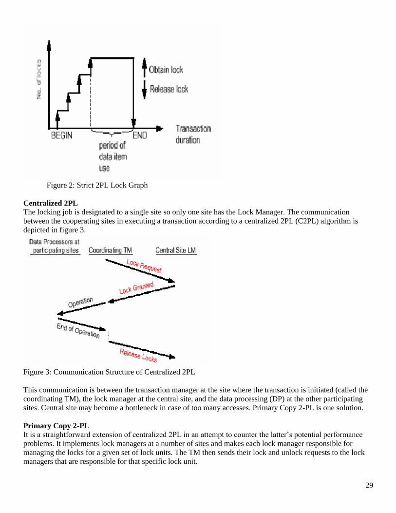
29

Figure 2: Strict 2PL Lock Graph

Centralized 2PL

The locking job is designated to a single site so only one site has the Lock Manager. The communication

between the cooperating sites in executing a transaction according to a centralized 2PL (C2PL) algorithm is

depicted in figure 3.

Figure 3: Communication Structure of Centralized 2PL

This communication is between the transaction manager at the site where the transaction is initiated (called the

coordinating TM), the lock manager at the central site, and the data processing (DP) at the other participating

sites. Central site may become a bottleneck in case of too many accesses. Primary Copy 2-PL is one solution.

Primary Copy 2-PL

It is a straightforward extension of centralized 2PL in an attempt to counter the latter’s potential performance

problems. It implements lock managers at a number of sites and makes each lock manager responsible for

managing the locks for a given set of lock units. The TM then sends their lock and unlock requests to the lock

managers that are responsible for that specific lock unit.

30

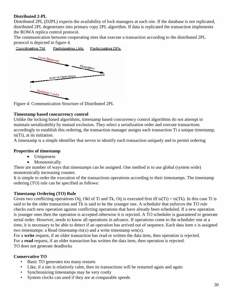
Distributed 2-PL

Distributed 2PL (D2PL) expects the availability of lock managers at each site. If the database is not replicated,

distributed 2PL degenerates into primary copy 2PL algorithm. If data is replicated the transaction implements

the ROWA replica control protocol.

The communication between cooperating sites that execute a transaction according to the distributed 2PL

protocol is depicted in figure 4.

Figure 4: Communication Structure of Distributed 2PL

Timestamp based concurrency control

Unlike the locking based algorithms, timestamp based concurrency control algorithms do not attempt to

maintain serializabiltiy by mutual exclusion. They select a serialization order and execute transactions

accordingly to establish this ordering, the transaction manager assigns each transaction Ti a unique timestamp,

ts(Ti), at its initiation.

A timestamp is a simple identifier that serves to identify each transaction uniquely and to permit ordering

Properties of timestamp

Uniqueness

Monotonically

There are number of ways that timestamps can be assigned. One method is to use global (system wide)

monotonically increasing counter.

It is simple to order the execution of the transactions operations according to their timestamps. The timestamp

ordering (TO) rule can be specified as follows:

Timestamp Ordering (TO) Rule

Given two conflicting operations Oij, Okl of Ti and Tk, Oij is executed first iff ts(Ti) < ts(Tk). In this case Ti is

said to be the older transaction and Tk is said to be the younger one. A scheduler that enforces the TO rule

checks each new operation against conflicting operations that have already been scheduled. If a new operation

is younger ones then the operation is accepted otherwise it is rejected. A TO scheduler is guaranteed to generate

serial order. However, needs to know all operations in advance. If operations come to the scheduler one at a

time, it is necessary to be able to detect if an operation has arrived out of sequence. Each data item x is assigned

two timestamps: a Read timestamp rts(x) and a write timestamp wts(x).

For a write request, if an older transaction has read or written the data item, then operation is rejected.

For a read request, if an older transaction has written the data item, then operation is rejected.

TO does not generate deadlocks

Conservative TO

• Basic TO generates too many restarts

• Like, if a site is relatively calm, then its transactions will be restarted again and again

• Synchronizing timestamps may be very costly

• System clocks can used if they are at comparable speeds

31

• In con-TO, operations are not executed immediately, but they are buffered

• Scheduler maintains queue for each TM.

• Operations from a TM are placed in relevant queue, ordered and executed later

• Reduces but does not eliminate restarts

Multiversion TO

• Another attempt to reduce the restarts

• Multiple versions of data items with largest r/w stamps are maintained.

• Read operation is performed from appropriate version

• Write is rejected if any older has read or written a data item

That was all about Pessimistic CC algorithms, now we move to Optimistic approaches.

Optimistic concurrency control

The execution of any operation of a transaction follows the sequence of phases:

Validation (V)

Read (R)

Computation (C)

Write (W)

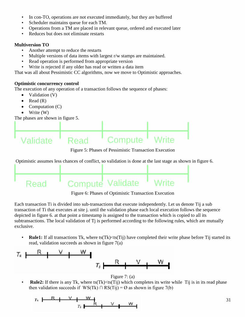
The phases are shown in figure 5.

Figure 5: Phases of Pessimistic Transaction Execution

Optimistic assumes less chances of conflict, so validation is done at the last stage as shown in figure 6.

Figure 6: Phases of Optimistic Transaction Execution

Each transaction Ti is divided into sub-transactions that execute independently. Let us denote Tij a sub

transaction of Ti that executes at site j. until the validation phase each local execution follows the sequence

depicted in figure 6. at that point a timestamp is assigned to the transaction which is copied to all its

subtransactions. The local validation of Tj is performed according to the following rules, which are mutually

exclusive.

• Rule1: If all transactions Tk, where ts(Tk)<ts(Tij) have completed their write phase before Tij started its

read, validation succeeds as shown in figure 7(a)

Figure 7: (a)

• Rule2: If there is any Tk, where ts(Tk)<ts(Tij) which completes its write while Tij is in its read phase

then validation succeeds if WS(Tk) ∩ RS(Tij) = Ø as shown in figure 7(b)

Validate Read Compute Write

Read Compute Validate Write

32

Figure 7: (b)

• Rule3: If Tk completes its read phase before Tij completes its read phase, then validation succeeds if

WS(Tk) ∩ RS(Tij) = Ø and

WS(Tk) ∩ WS(Tij) = Ø

Need more storage for the validation tests

• Repeated failure for longer transactions.

Deadlock Management

• Locking based concurrency control generates deadlock

• T1 waits for data item being held by T2, and other way round as shown in figure 8.

• A tool in analyzing deadlocks is a Wait-for Graph (WFG).

• A WFG represents the relationship between transactions waiting for each other to release data items.

Figure 8: Deadlock

There are three methods for handling deadlocks:

Prevention

Avoidance

Detection and resolution

Summary

We have discussed the locking based concurrency control and the timestamp ordering based on concurrency

control.


Course Code: CS712

T2 T5 T3

T7

33


Lecture No: 30


- Locking based CC

- Timestamp ordering based CC

- Concluded TM

In this lecture:

- Basic Concepts of Query Optimization

- QP in centralized and Distributed DBs

Introduction

Distributed database design is of major importance for query processing since the definition of fragments is

based on the objective of increasing reference locality and sometimes parallel execution for the most important

queries. The role of distributed query processor is to map a high level query on a distributed database into a

sequence of database operations on relation fragments.

Query processing problem

The main function of a relational query processor is to transform a high level query into an equivalent lower

level query. The low level query actually implements the execution strategy for the query. The transformation

must achieve both correctness and efficiency. It is correct if the low level query has the same semantics as the

original query, i.e. if both queries produce the same result.

Example

Consider the following relations

• EMP(eNo, eName, title)

• ASG(eNo, pNo, resp, dur)

• PROJ(pNo, pName, budget, loc)

Query: Get the names of employees who are managing a project

34

SELECT eName

FROM EMP, ASG

WHERE EMP.eNo = ASG.eNo

AND resp = ‘Manager’

Two equivalent relational algebra queries that are correct transformation of the query above are

• eName(resp=‘Manager’ ^ EMP.eNo = ASG.eNo) (EMPxASG)

And

• eName(EMP ⋈ (resp=‘Manager’ (ASG)))

It is obvious that the second query, which avoids the Cartesian product of EMP and ASG consumes much less

computing resource than the first and thus should be retained.

Centralized QP

In a centralized query execution strategies can be well expressed in an extension of relational algebra. The main

role of a centralized query processor is to choose, for a given query, the best relational algebra query among all

equivalent ones.

Distributed QP

In distributed system relational algebra is not enough to express execution strategies. It must be supplemented

with operations for exchanging data between sites.

The distributed QP must also select the best sites to process data, and possibly the way data should be

transformed. This increases the solution space from which to choose the distributed execution strategy, making

distributed query processing significantly more difficult.

Example

Consider the same query in of previous example

Suppose EMP and ASG are Horizontally Fragmented as

• EMP1 = eNo ≤ ‘E3’ (EMP)

• EMP2 = eNo > ‘E3’ (EMP)

• ASG1 = eNo ≤ ‘E3’ (ASG)

• ASG2 = eNo > ‘E3’ (ASG)

Further suppose these fragments are stored at site 1, 2, 3 and 4 and result at site 5

35

Figure 1: Equivalent Distributed Execution Strategies

Two equivalent distributed execution strategies for the query are shown in figure 1. an arrow from site I to site j

labeled with R indicates that relation R is transferred from site I to site j.

Strategy A exploits the fact that relations EMP and ASG are fragmented the same way in order to perform the

select and join operation in parallel.

Strategy B centralizes all the operand data at the result site before processing the query as shown in figure 1.

To evaluate the resource consumption of these two strategies we use a cost model. Let’s Assume

• size(EMP)

• size(ASG)

400

1000

• tuple access cost

• tuple transfer cost

1 unit

10 units

• There are 20 Managers

• Data distributed evenly at all sites

Strategy 1

ASC1’=resp = ‘Manager(ASG1)

EMP1’=EMP1 ⋈(ASG1’)

Site 1

Site 3

ASC2’=resp = ‘Manager(ASG2)

EMP2’=EMP2 ⋈(ASG2’)

Site 2

Site 4

ASG1’ ASG2’

result = EMP1’ U EMP2’ Site 5

EMP1’ EMP2’

result = (EMP1 U EMP2) ⋈ eNo

resp = ‘Manager’ (ASG1 U ASG2)

Site 1 Site 2 Site 3 Site 4

ASG1 ASG2 EMP

1 EMP

2

36

The cost of strategy A can be derived as follows:

• produce ASG': 20*1 20

• transfer ASG' to the sites of E: 20 * 10 200

• produce EMP': (10+10) *1*2 40

• transfer EMP' to result site: 20*10 200

Total 460

Strategy 2

The cost of strategy B can be derived as follows:

• Transfer EMP to site 5: 400 * 10 4000

• Transfer ASG to the site 5 1000 * 10 10000

• Produce ASG‘ by selecting ASG 1000

• Join EMP and ASG’ 8000

Total 23000

In strategy B we assumed that the access methods to relations EMP an ASG based on attributes RESP and ENO

are lost because of data transfer. This is reasonable assumption.

Strategy A is better by a factor of 50, which is quite significant. It provides better distribution of wok among

sites. The difference would be higher if we assumed slower communication and/or high degree of

fragmentation.

Objective of Query Processing

The objective of query processing in a distributed context is to transform a high level query on a distributed

database. An important of query processing is query optimization.

Query Optimization

Many execution strategies are correct transformations of the same high level query the one that optimizes

(minimizes) resource consumption should be retained.

A good measure of resource consumption is the total cost that will be incurred in processing the query. Total

cost is the sum of all times incurred in processing the operations of the query at various sites.

In a distributed database system, the total cost to be minimized includes CPU, I/O and communication costs.

The first two components (I/O and CPU costs) are the only factors considered by centralized DBMSs.

Communication Cost will dominate in WAN but not that dominant in LANs. Query optimization can also

maximize throughput

Operators’ Complexity

Relational algebra is the output of query processing. The complexity of relational algebra operations, which

directly affects their execution time, dictates some principles useful to a query processor. Figure 2 shows the

complexity of unary and binary operations.

• Select, Project (without duplicate elimination)

O(n)

• Project (with duplicate elimination), Group

O(nlogn)

• Join, Semi-Join, Division, Set Operators

O(nlog n)

37

• Cartesian Product O(n2)

Figure 2: Complexity of Unary and Binary Operations

Characterization of Query Processors

There are some characteristics of query processors that can be used as a basis for comparison.

• Types of Optimization

– Exhaustive search for the cost of each strategy to find the most optimal one

– May be very costly in case of multiple options and more fragments

– Heuristics

• Optimization Timing

– Static: during compilation

• Size of intermediate tables not known always

• Cost justified with repeated execution

– Dynamic: during execution

• Intermediate tables’ size known

• Re-optimization may be required

• Statistics

– Relation/Fragment: Cardinality, size of a tuple, fraction of tuples participating in a join with

another relation

– Attribute: cardinality of domain, actual number of distinct values

• Decision Sites

– Centralized: simple, need knowledge about the entire distributed database

– Distributed: cooperation among sites to determine the schedule, need only local information

– Hybrid: one site determines the global schedule, each site optimizes the local sub queries

Summary

We have discussed the basic concepts of query processing and the query optimization in centralized and

distributed databases.


Course Code: CS712


Lecture No: 31

38


- Basic concepts of query optimization

- Query processing in centralized and distributed DBs

In this lecture:

- Query decomposition

- Its different phases

39

Query Decomposition: Query decomposition transforms an SQL (relational calculus) query into relational algebra query on global

relations. The information needed for this transformation is found in the global conceptual schema.

Steps in query decomposition:

It consists of four phases:

1) Normalization:

Input query can be complex depending on the facilities provided by the language. The goal of normalization is

to transform the query to a normalized form to facilitate further processing. This process includes the lexical

and analytical analysis and the treatment of WHERE clause. There are two possible normal forms.

Conjunctive NF:

This is a conjunction (∧ predicate) of disjunctions (∨ predicates) as follows:

(p11 ∨p12 ∨…∨p1n) ∧…∧(pm1 ∨pm2 …∨pmn)

Disjunctive NF:

This is disjunction (∨ predicate) of conjunctions (∧ predicates) as follows:

(p11 ∧p12∧…∧p1n) ∨…∨(pm1∧pm2 ∧…∧pmn)

The transformation of the quantifier-free predicate is using equivalence rules.

Equivalence rules: Some of equivalence rules are:

1. p1∧ p2 ⇔ p2∧ p1

2. p1∨ p2 ⇔ p2∨ p1

3. p1 ∧ (p2∧ p3) ⇔ (p1∧p2) ∧ p3

4. p1 ∨ (p2∨ p3) ⇔ (p1∨p2) ∨ p3

5. ¬(¬ p1) ⇔ p

…

Example

The query expressed in SQL is

SELECT ENAME

FROM EMP,ASG

WHERE EMP.ENO=ASG.ENO

AND ASG.PNO=’P1’

AND DUR=12

OR DUR=24

The qualification in conjunctive NF is

EMP.ENO = ASG.ENO ∧ ASG.PNO=”P1” ∧ (DUR=12 ∨ DUR=24)

The qualification in disjunctive NF is

(EMP.ENO = ASG.ENO ∧ ASG.PNO=”P1” ∧ DUR=12) ∨

(EMP.ENO = ASG.ENO ∧ ASG.PNO=”P1” ∧ DUR=24)

2) Analysis:

Query analysis enables rejection of normalized queries for which further processing is either impossible or

necessary. The main reasons for rejection are that the query is type incorrect or semantically incorrect.

Type incorrect

If any of its attribute or relation names are not defined in the global schema

If operations are applied to attributes of the wrong type

Semantically incorrect

Components do not contribute in any way to the generation of the result

Only a subset of relational calculus queries can be tested for correctness

Those that do not contain disjunction and negation

40

To detect through Connection graph (query graph) and Join graph

Query Graph

This graph is used for most queries involving select, project, and join operations. In a graph, one node

represents the result relation and any other node represents an operand relation. An edge between two nodes that

are not results represents a join, whereas an edge whose destination node is the result represents a project.

Example

Consider the following query in SQL;

SELECT ENAME, RESP

FROM EMP, ASG, PROJ

WHERE EMP.ENO = ASG.ENO

AND ASG.PNO = PROJ.PNO

AND PNAME = “CAD/CAM”

AND DUR >= 36

AND TITLE = “PROGRAMMER”

Figure1: Query graph

Join graph

This is the graph in which only joins are considered.

Figure2: Join graph

If the query graph is not connected, the query is wrong.

Example

Consider the SQL query;

SELECT ENAME, RESP

FROM EMP, ASG, PROJ

WHERE EMP.ENO = ASG.ENO

AND PNAME = “CAD/CAM”

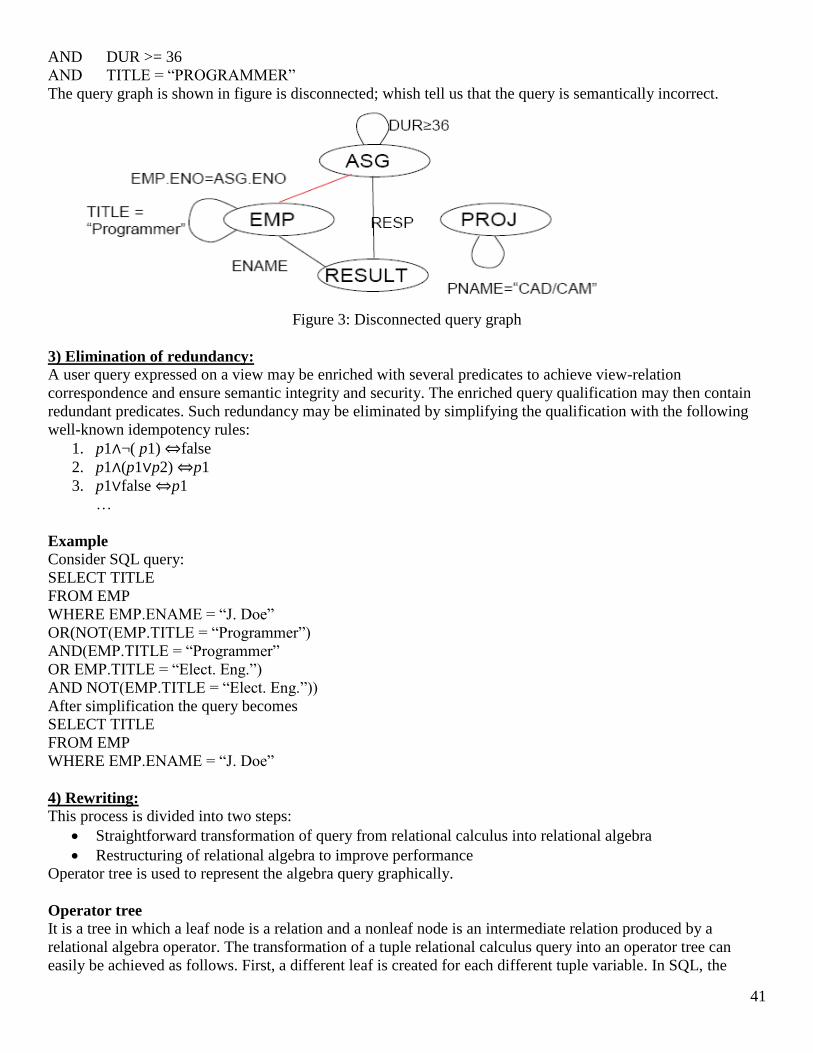
41

AND DUR >= 36

AND TITLE = “PROGRAMMER”

The query graph is shown in figure is disconnected; whish tell us that the query is semantically incorrect.

Figure 3: Disconnected query graph

3) Elimination of redundancy:

A user query expressed on a view may be enriched with several predicates to achieve view-relation

correspondence and ensure semantic integrity and security. The enriched query qualification may then contain

redundant predicates. Such redundancy may be eliminated by simplifying the qualification with the following

well-known idempotency rules:

1. p1∧¬( p1) ⇔false

2. p1∧(p1∨p2) ⇔p1

3. p1∨false ⇔p1

…

Example

Consider SQL query:

SELECT TITLE

FROM EMP

WHERE EMP.ENAME = “J. Doe”

OR(NOT(EMP.TITLE = “Programmer”)

AND(EMP.TITLE = “Programmer”

OR EMP.TITLE = “Elect. Eng.”)

AND NOT(EMP.TITLE = “Elect. Eng.”))

After simplification the query becomes

SELECT TITLE

FROM EMP

WHERE EMP.ENAME = “J. Doe”

4) Rewriting:

This process is divided into two steps:

Straightforward transformation of query from relational calculus into relational algebra

Restructuring of relational algebra to improve performance

Operator tree is used to represent the algebra query graphically.

Operator tree

It is a tree in which a leaf node is a relation and a nonleaf node is an intermediate relation produced by a

relational algebra operator. The transformation of a tuple relational calculus query into an operator tree can

easily be achieved as follows. First, a different leaf is created for each different tuple variable. In SQL, the

42

leaves are immediately available in the FROM clause. Second, the root node is created as a project operation

and these are found in SELECT clause. Third, the SQL WHERE clause is translated into the sequence of

relational operations (select, join, union, etc.).

Example

Consider the SQL query:

SELECT ENAME

FROM PROJ, ASG, EMP

WHERE ASG.ENO = EMP.ENO


AND ENAME = “J.DOE”

AND PROJ.PNAME = “CAD/CAM”

AND (DUR = 12 OR DUR = 24)

Figure 4: Example of operator tree

By applying transformation rules many different trees may be found.

Transformation Rules

Commutativity of binary operations

R × S ⇔ S × R

R S ⇔ S R

Associativity of binary operations

( R × S) × T ⇔ R × (S × T)

(R S) T ⇔ R (S T)

There are other rules that we will discuss in next lecture.

Summary:

Query processing has four different phases and the first phase is the Query Decomposition. The steps of query

decomposition are normalization, analysis, simplification and rewriting. Our goal in every process is same to

produce a correct and efficient query. We have studied an equivalence rules, idempotency rules and some of

transformation rules.

43


Course Code: CS712


Lecture No: 32


- Query decomposition

- Its different phases

In this lecture:

- Final phase of Query decomposition

- Next phase of query optimization: Data localization

44

Transformation Rules:

First two transformation rules have discussed in previous lecture and we are going to discuss other rules.

Idempotence of unary operations

o ΠA’(ΠA’’(R)) ΠA’(R)

o σp1(A1)(σp2(A2)(R)) σp1(A1) ∧ p2(A2)(R)

Commuting selection with projection

o A1, ….,An(p(Ap)(R)) A1, ….,An((p(Ap) A1, ….,An, Ap(R)))

Commuting selection with binary operations

o σp(A)(R×S) (σp(A) (R)) ×S

o σp(Ai)(R(Aj,Bk)S) (σp(Ai) (R)) (Aj,Bk)S

Commuting projection with binary operations

o ΠC(R×S) ΠA’(R) ×ΠB’(S)

o ΠC(R(Aj,Bk)S) ΠA’(R) (Aj,Bk)ΠB’(S)

These rules enables the generation of many equivalent trees. In optimization phase, one can imagine comparing

all possible trees based on their predicted cost. The excessively large number of possible trees makes this

approach unrealistic. The above rules can be used to restructure the tree in a systematic way so that the bad

operator trees are eliminated. These rules can be used in four different ways:

They allow the separation of unary operations, simplifying the query expression.

Unary operations on the same relation may be grouped together

Unary operations can be commuted with binary operations

Binary operations can be ordered

Example

Consider the SQL query:

SELECT ENAME

FROM PROJ, ASG, EMP

WHERE ASG.ENO = EMP.ENO


AND ENAME = “Saleem”

AND PROJ.PNAME = “CAD/CAM”

AND (DUR = 12 OR DUR = 24)

45

Figure1: Equivalent operator tree

Figure 2: Rewritten operator tree

This concludes query decomposition and restructuring. Now we move towards the second phase of query

optimization or query processing that is Data Localization.

Data Localization:

The localization layer translates an algebraic query on global relations into an algebraic query expressed on

physical fragments. Localization uses information stored in the fragment schema. Fragmentation is defined

ASG PROJ EMP

x

⋈ pNo^eNo

(pName = ‘CAD/CAM’)^ (dur = 12 v dur = 24)^ eName ’Saleem’

eName

PROJ ASG EMP

pName = ‘CAD/CAM’ dur=12 v dur = 24 eName != ‘Saleem’

pNo’ pNo, eNo eNo, eName

pNo, eName

eName

46

through fragmentation riles, which can be expressed as relational queries. A global relation can be reconstructed

by applying the reconstruction rules and deriving a relational algebra program whose operands are the

fragments, this process is called localization program.

A native way to localize a distributed query is to generate a query where each global relation is substituted by

its localization program. This can be viewed as replacing the leaves of the operator tree of distributed query

with sub trees corresponding to the localization programs. The query obtained in this way is called a generic

query. Here we are going to present reduction techniques for each type of fragmentation.

Reduction for primary horizontal fragmentation:

The horizontal fragmentation function distributes a relation based on selection predicates. Consider an example:

Example:

Relation EMP(eNo, eName, title) can be split into three horizontal fragments.

• EMP1 = eNo ≤ ‘E3’ (EMP)

• EMP2 = ’E3’<eNo ≤ ‘E6’ (EMP)

• EMP3 = eNo > ‘E6’ (EMP)

The localization program for a horizontally fragmented relation is the union of fragments.e.g.

EMP = EMP1 U EMP2 U EMP3

Horizontal fragmentation can be exploited to simplify both selection and join operations.

Reduction with selection:

Selections on fragments that have a qualification contradicting the qualification of the fragmentation rule

generate empty relations. The rule can be stated as:

Rule 1:

pi (Rj) = Ø if ∀x in R: (pi(x) ^ pj(x))

where pi and pj are selection predicates, x denotes a tuple, and p(x) denotes “predicate p holds for x”.

Example:

Consider a query

SELECT *

FROM EMP

WHERE ENO = ‘E7’

Generic query Reduced query

Figure 3: Reduction for horizontal fragmentation (with selection)

Reduction with join:

EMP1 EMP2 EMP3

U

eNo = ‘E7’

EMP3

eNo = ‘E7’

47

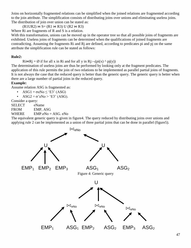
Joins on horizontally fragmented relations can be simplified when the joined relations are fragmented according

to the join attribute. The simplification consists of distributing joins over unions and eliminating useless joins.

The distribution of join over union can be stated as:

(R1UR2) ⋈ S= (R1 ⋈ R3) U (R2 ⋈ R3)

Where Ri are fragments of R and S is a relation.

With this transformation, unions can be moved up in the operator tree so that all possible joins of fragments are

exhibited. Useless joins of fragments can be determined when the qualifications of joined fragments are

contradicting. Assuming the fragments Ri and Rj are defined, according to predicates pi and pj on the same

attribute the simplification rule can be stated as follows:

Rule2:

Ri⋈Rj = Ø if for all x in Ri and for all y in Rj:(pi(x) ^ pj(y))

The determination of useless joins are thus be performed by looking only at the fragment predicates. The

application of this rule permits the join of two relations to be implemented as parallel partial joins of fragments.

It is not always the case that the reduced query is better than the generic query. The generic query is better when

there are a large number of partial joins in the reduced query.

Example:

Assume relation ASG is fragmented as:

• ASG1 = eNo ≤ ‘E3’ (ASG)

• ASG2 = ’eNo > ‘E3’ (ASG).

Consider a query:

SELECT eName

FROM EMP, ASG

WHERE EMP.eNo = ASG. eNo

The equivalent generic query is given in figure4. The query reduced by distributing joins over unions and

applying rule 2 can be implemented as a union of three partial joins that can be done in parallel (figure5).

Figure 4: Generic query

EMP1 EMP2 EMP3

U

⋈eNo

ASG1 ASG2

U

EMP1

U

⋈eNo

ASG1 EMP2

⋈eNo

ASG2 EMP3

⋈eNo

ASG2

48

Figure 5: Reduced query

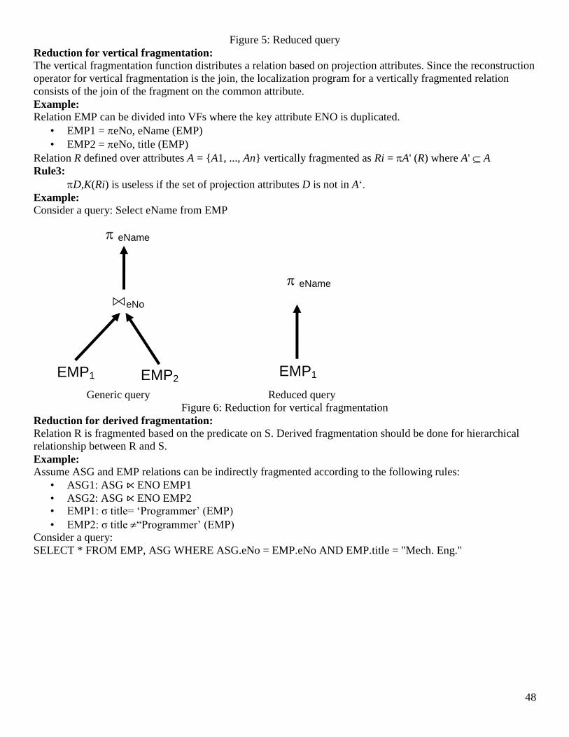
Reduction for vertical fragmentation:

The vertical fragmentation function distributes a relation based on projection attributes. Since the reconstruction

operator for vertical fragmentation is the join, the localization program for a vertically fragmented relation

consists of the join of the fragment on the common attribute.

Example:

Relation EMP can be divided into VFs where the key attribute ENO is duplicated.

• EMP1 = eNo, eName (EMP)

• EMP2 = eNo, title (EMP)

Relation R defined over attributes A = {A1, ..., An} vertically fragmented as Ri = A' (R) where A' A

Rule3:

D,K(Ri) is useless if the set of projection attributes D is not in A‘.

Example:

Consider a query: Select eName from EMP

Generic query Reduced query

Figure 6: Reduction for vertical fragmentation

Reduction for derived fragmentation:

Relation R is fragmented based on the predicate on S. Derived fragmentation should be done for hierarchical

relationship between R and S.

Example:

Assume ASG and EMP relations can be indirectly fragmented according to the following rules:

• ASG1: ASG ⋉ ENO EMP1

• ASG2: ASG ⋉ ENO EMP2

• EMP1: σ title= ‘Programmer’ (EMP)

• EMP2: σ title “Programmer’ (EMP)

Consider a query:

SELECT * FROM EMP, ASG WHERE ASG.eNo = EMP.eNo AND EMP.title = "Mech. Eng."

EMP1

⋈eNo

EMP2

eName

EMP1

eName

49

Generic query

Query after pushing selection down

Figure 7: Query after moving unions up

ASG1

⋈eNo

U

ASG2 EMP1 EMP2

U

title = ‘Mech

ASG1

⋈eNo

U

ASG2 EMP2

title = ‘Mech Eng.’

ASG1

⋈eNo

U

EMP2

ASG2

EMP2

title = ‘Mech Eng.’ title = ‘Mech Eng.’

⋈eNo

50

Figure 8: Reduced query after eliminating the left sub tree

Summary

We have discussed final phase of Query decomposition and next phase of query optimization i.e. Data

localization.


Course Code: CS712


Lecture No: 33

ASG2 EMP2

title = ‘Mech Eng.’

⋈eNo

51


- Final phase of QD

- Data Localization: for HF, VF and DF

In this lecture:

- Data Localization for Hybrid Fragmentation

- Query Optimization

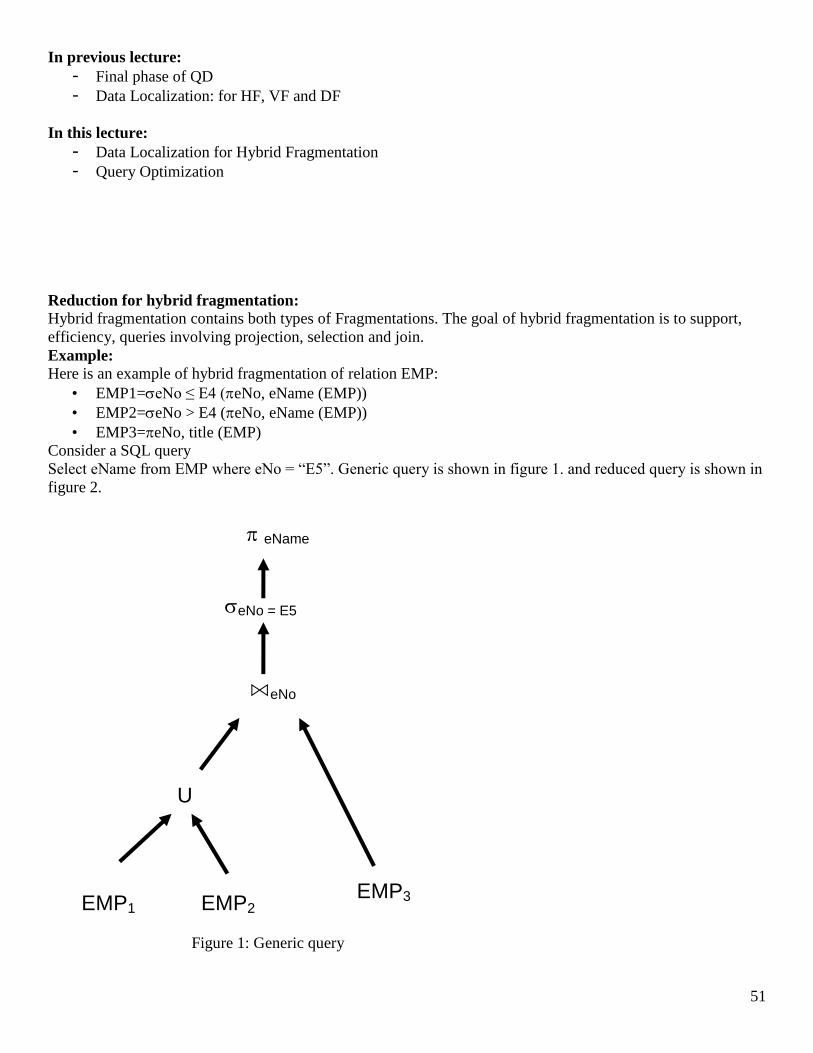
Reduction for hybrid fragmentation:

Hybrid fragmentation contains both types of Fragmentations. The goal of hybrid fragmentation is to support,

efficiency, queries involving projection, selection and join.

Example: Here is an example of hybrid fragmentation of relation EMP:

• EMP1=eNo ≤ E4 (eNo, eName (EMP))

• EMP2=eNo > E4 (eNo, eName (EMP))

• EMP3=eNo, title (EMP)

Consider a SQL query

Select eName from EMP where eNo = “E5”. Generic query is shown in figure 1. and reduced query is shown in

figure 2.

Figure 1: Generic query

EMP1

⋈eNo

EMP2

eName

EMP3

U

eNo = E5

52

Figure 2: Reduced query

Summary of what we have done so far

• Query Decomposition: generates an efficient query in relational algebra

– Normalization, Analysis, Simplification, Rewriting

• Data Localization: applies global query to fragments; increases optimization level

• So, next is the cost-based optimization

Query optimization:

Query optimization refers to the process of producing a query execution plan (QEP) which represents an

execution strategy for the query. The selected plan minimizes an objective cost functions. A query optimizer,

the software module that performs query optimization, is usually seen as three components:

1. Search space

2. Search strategy

3. Cost model

1) Search Space

The search space is the set of alternative execution plans to represent the input query. These plans are

equivalent, in the sense that the same result but they differ on execution order of operations and the way these

operations are implemented. Search space consists of equivalent query trees produced using transformation

rules. Optimizer concentrates on join trees, since join cost is the most effective.

Example:

Select eName, resp

From EMP, ASG, PROJ where EMP.eNo = ASG. eNo and ASG.pNo = PROJ.pNo.

The Equivalent join trees are shown in figure 3.

EMP2

eName

eNo = E5

53

Figure 3: Equivalent join trees

For a complex query the number of equivalent operator trees can be very high. For instance, the number of

alternative join trees that can be produced by applying the commutativity and associativity rules is O(N!) for N

relations. Query optimizers restrict the size of the search space they consider. Two restrictions are:

1- Heuristics

EMP

⋈eNo

ASG

PROJ

⋈pNo

PROJ

⋈pNo

ASG

EMP

⋈eNo

EMP

x

PROJ

ASG

⋈pNo, eNo

54

- Most common heuristic is to perform selection and projection on base relations

- Another is to avoid Cartesian product

2- Shape of join Tree

Two types of join trees are distinguished:

- Linear Tree: At least one node for each operand is a base relation

- Bushy tree: May have operators with no base relations as operands (both operands are intermediate

relations)

2) Search Strategy

• Most popular search strategy is Dynamic Programming

• That starts with base relations and keeps on adding relations calculating cost

• DP is almost exhaustive so produces best plan

• Too expensive with more than 5 relations

• Other option is Randomized strategy

• Do not guarantee best

3) Cost Model:

An optimizer’s cost model includes cost functions to predict the cost of operators, statistics, and base data and

formulas to evaluate the sizes of intermediate results.

Cost function: • The cost of distributed execution strategy can be expressed with respect to either the total time or the

response time.

• Total time = CPU time + I/O time + tr time

• In WAN, major cost is tr time

• Initially ratios were 20:1 for tr and I/O, for LAN it is 1:1.6

• Response time = CPU time + I/O time + tr time

• TCPU = time for a CPU insts

• TI/O = a disk I/O

• TMSG = fixed time for initiating and recv a msgs

• TTR = transmit a data unit from one site to another

Example:

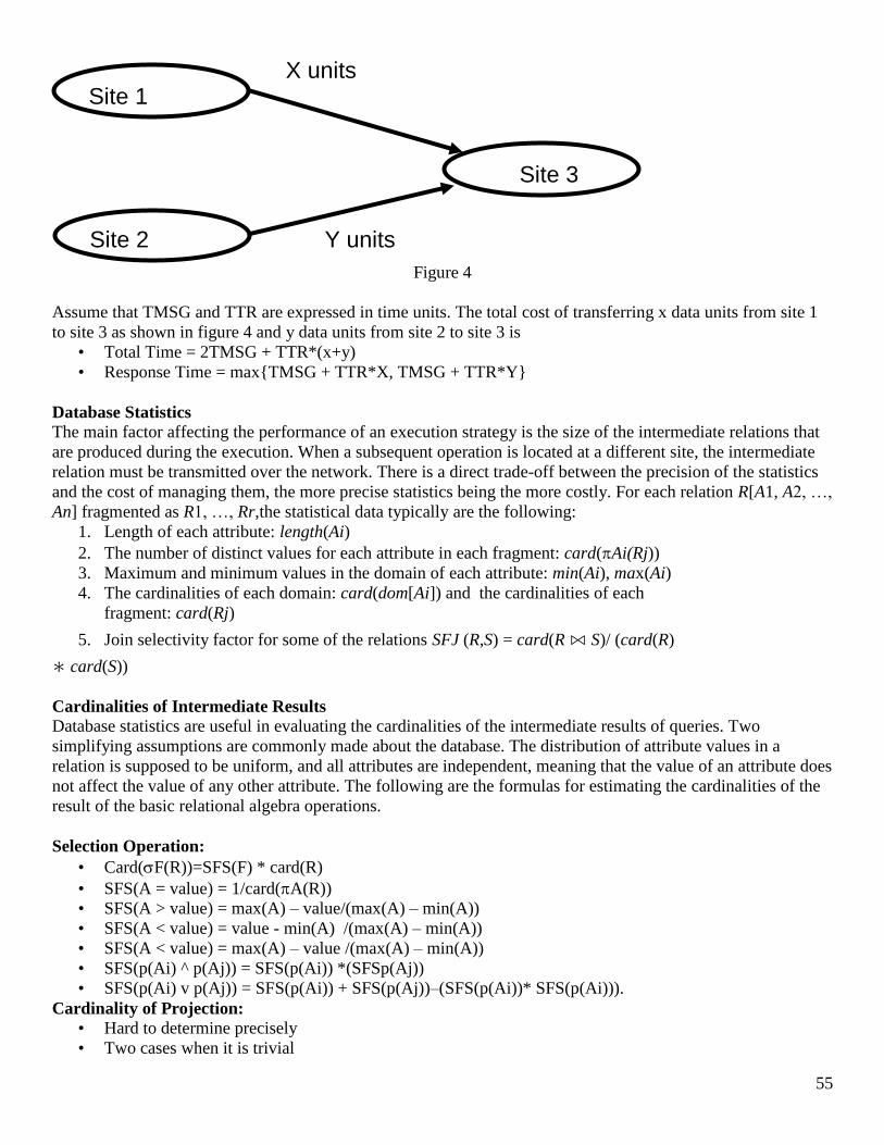
55

Figure 4

Assume that TMSG and TTR are expressed in time units. The total cost of transferring x data units from site 1

to site 3 as shown in figure 4 and y data units from site 2 to site 3 is

• Total Time = 2TMSG + TTR*(x+y)

• Response Time = max{TMSG + TTR*X, TMSG + TTR*Y}

Database Statistics

The main factor affecting the performance of an execution strategy is the size of the intermediate relations that

are produced during the execution. When a subsequent operation is located at a different site, the intermediate

relation must be transmitted over the network. There is a direct trade-off between the precision of the statistics

and the cost of managing them, the more precise statistics being the more costly. For each relation R[A1, A2, …,

An] fragmented as R1, …, Rr,the statistical data typically are the following:

1. Length of each attribute: length(Ai)

2. The number of distinct values for each attribute in each fragment: card(Ai(Rj))

3. Maximum and minimum values in the domain of each attribute: min(Ai), max(Ai)

4. The cardinalities of each domain: card(dom[Ai]) and the cardinalities of each

fragment: card(Rj)

5. Join selectivity factor for some of the relations SFJ (R,S) = card(R ⋈ S)/ (card(R)

∗ card(S))

Cardinalities of Intermediate Results

Database statistics are useful in evaluating the cardinalities of the intermediate results of queries. Two

simplifying assumptions are commonly made about the database. The distribution of attribute values in a

relation is supposed to be uniform, and all attributes are independent, meaning that the value of an attribute does

not affect the value of any other attribute. The following are the formulas for estimating the cardinalities of the

result of the basic relational algebra operations.

Selection Operation:

• Card(F(R))=SFS(F) * card(R)

• SFS(A = value) = 1/card(A(R))

• SFS(A > value) = max(A) – value/(max(A) – min(A))

• SFS(A < value) = value - min(A) /(max(A) – min(A))

• SFS(A < value) = max(A) – value /(max(A) – min(A))

• SFS(p(Ai) ^ p(Aj)) = SFS(p(Ai)) *(SFSp(Aj))

• SFS(p(Ai) v p(Aj)) = SFS(p(Ai)) + SFS(p(Aj))–(SFS(p(Ai))* SFS(p(Ai))).

Cardinality of Projection:

• Hard to determine precisely

• Two cases when it is trivial

Site 1

Site 2

Site 3

X units

Y units

56

1- When a single attribute A,

card(A(R)) = card (A)

2- When PK is included

card(A(R)) = card (R)

Cartesian Product:

• card(RxS) = card (R) * card(S)

Cardinality of Join:

• No general way to test without additional information

• In case of PK/FK combination

Card(R ⋈ S) = card (S)

Semi Join:

• SFSJ(R ⋉AS)= card(A(S))/ card(dom[A])

• card(R ⋉AS) = SFSJ(S.A) * card(R)

Union:

• Hard to estimate

• Limits possible which are card(R) + card(S) and max{card (R) + card (S))

Difference:

• Like Union, card (R) for (R-S), and 0

Centralized Query Optimization

A distributed query is transformed into local ones, each of which is presented in centralized way. Distributed

query optimization techniques are often extensions of the techniques for centralized systems. Centralized query

optimization is simpler problem; the minimization of communication costs makes distributed query

optimization more complex. Two popular query optimization techniques:

• INGRES

• Dynamic optimization

• Recursively breaks into smaller ones

• System R

• Static optimization

• Based on exhaustive search using statistics about the database

Maximum DBMs uses static approach s here our focus is on static approach that is adopted by system R.

Summary

We have discussed the final phase of data localization the concepts of query optimization and the components

of query optimization: search space, cost model and search strategy. For cost calculation database information

and statistics are required.

57


Course Code: CS712


Lecture No: 34


- Concluded Data Localization


o Components: Search space, cost model, search strategy

o Search space consists of equivalent query trees

o Search strategy could be static, dynamic or randomized

o Cost model sees response and total times…

o Transmission cost is the most important

o Another major factor is size of intermediate tables

o Database statistics are used to evaluate size of intermediate tables

o Selectivity factor, card, size are some major figures

In this lecture:


- Centralized Query optimization

o Best access path

o Join Processing

- Query optimization in Distributed Environment

Centralized Query Optimization:

System R:

System R performs static query optimization based on the exhaustive search of the solution space. The input to

the optimizer of system R is a relational algebra tree resulting from the decomposition of an SQL query. The

output is an execution plan that implements the “optimal” relational algebra tree.

58

The optimizer assigns a cost to every candidate tree and retains the one with the smallest cost. The candidate

trees are obtained by a permutation of the join orders of the n relations of the query using the commutativity and

associativity rules. To limit the overhead of optimization, the number of alternative trees is reduced using

dynamic programming. The set of alternative strategies is considered dynamically so that when two joins are

equivalent by commutativity, only the cheapest one is kept.

Two major steps in Optimization Algorithm

Best access path for individual relation with predicate

The best join ordering is eliminated

An important decision with either join method is to determine the cheapest access path to internal relation.

There are two methods:

1) Nested loops

2) Merge join

1) Nested loops:

It composes the product of the two relations. For each tuple of the external relation, the tuples of the internal

relation that satisfy the join predicate are retrieved one by one to form the resulting relation. An index on the

join attribute is very efficient access path for internal relation. In the absence of an index, for relations of n1 and

n2 pages resp. this algorithm has a cost proportional to n1*n2 which may be prohibitive if n1 & n2 are high.

2) Merge join:

If consists of merging two sorted relations on the join attribute as shown in figure 1. Indices on the join attribute

may be used as access paths. If the join criterion is equally the cost of joining two relations n1 and n2 pages,

resp. is proportional to n1+n2. this method is always chosen when there is an equi join, and when the relations

are previously sorted.

Example:

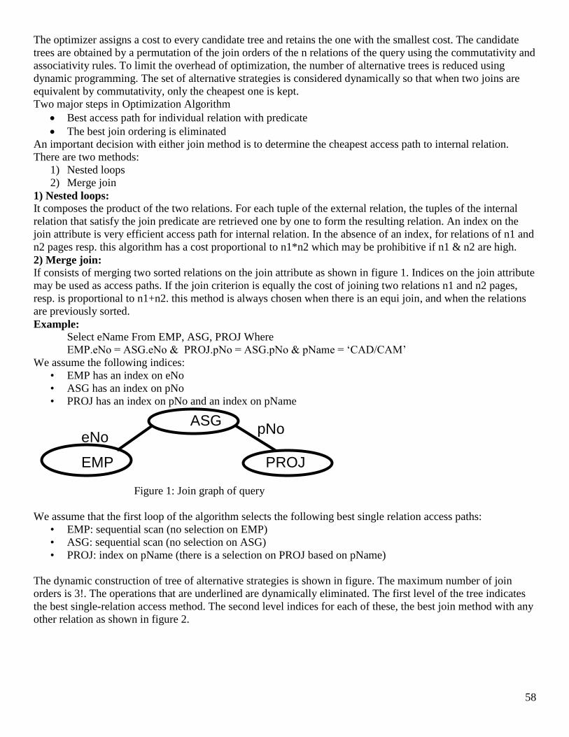
Select eName From EMP, ASG, PROJ Where

EMP.eNo = ASG.eNo & PROJ.pNo = ASG.pNo & pName = ‘CAD/CAM’

We assume the following indices:

• EMP has an index on eNo

• ASG has an index on pNo

• PROJ has an index on pNo and an index on pName

Figure 1: Join graph of query

We assume that the first loop of the algorithm selects the following best single relation access paths:

• EMP: sequential scan (no selection on EMP)

• ASG: sequential scan (no selection on ASG)

• PROJ: index on pName (there is a selection on PROJ based on pName)

The dynamic construction of tree of alternative strategies is shown in figure. The maximum number of join

orders is 3!. The operations that are underlined are dynamically eliminated. The first level of the tree indicates

the best single-relation access method. The second level indices for each of these, the best join method with any

other relation as shown in figure 2.

EMP PROJ

eNo pNo

ASG

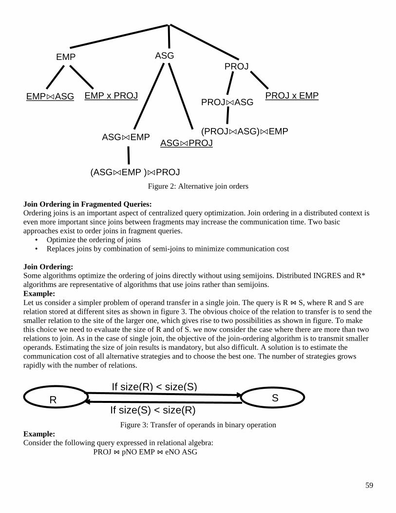
59

Figure 2: Alternative join orders

Join Ordering in Fragmented Queries:

Ordering joins is an important aspect of centralized query optimization. Join ordering in a distributed context is

even more important since joins between fragments may increase the communication time. Two basic

approaches exist to order joins in fragment queries.

• Optimize the ordering of joins

• Replaces joins by combination of semi-joins to minimize communication cost

Join Ordering: Some algorithms optimize the ordering of joins directly without using semijoins. Distributed INGRES and R*

algorithms are representative of algorithms that use joins rather than semijoins.

Example:

Let us consider a simpler problem of operand transfer in a single join. The query is R ⋈ S, where R and S are

relation stored at different sites as shown in figure 3. The obvious choice of the relation to transfer is to send the

smaller relation to the site of the larger one, which gives rise to two possibilities as shown in figure. To make

this choice we need to evaluate the size of R and of S. we now consider the case where there are more than two

relations to join. As in the case of single join, the objective of the join-ordering algorithm is to transmit smaller

operands. Estimating the size of join results is mandatory, but also difficult. A solution is to estimate the

communication cost of all alternative strategies and to choose the best one. The number of strategies grows

rapidly with the number of relations.

Figure 3: Transfer of operands in binary operation

Example:

Consider the following query expressed in relational algebra:

PROJ ⋈ pNO EMP ⋈ eNO ASG

EMP x PROJ

EMP ASG

PROJ

EMP⋈ASG

ASG⋈EMP

PROJ x EMP PROJ⋈ASG

ASG⋈PROJ

(ASG⋈EMP )⋈PROJ

(PROJ⋈ASG)⋈EMP

R

If size(R) < size(S) S

If size(S) < size(R)

60

Whose join graph is given in figure 4, we have made certain assumptions about the locations of three relations.

This query can be executed in at least five different ways. We describe these strategies by the following

programs, where (R site j) stands for “relation R is transferred to site j”.

Figure 4: Join graph of distributed query

Strategy 1:

EMPsite2, site2 computes EMP’= EMP ⋈ ASGsite3 computes EMP’ ⋈ PROJ

Strategy 2:

ASGsite1, site1 computes EMP’= EMP ⋈ ASGsite3 computes EMP’ ⋈ PROJ

Strategy 3:

ASGsite3, site3 computes ASG’= PROJ ⋈ ASGsite1

Strategy 4:

PROJsite2, site2 computes PROJ’= PROJ ⋈ ASGsite1 computes EMP ⋈ PROJ’

Strategy 5:

EMP, PROJsite2, site2 computes PROJ ⋈ ASG ⋈ EMP

To select one of these programs, the following sizes must be known or predicted : size(EMP),

size(ASG),size(PROJ),size(EMP ⋈ ASG), and size(ASG ⋈ PROJ). If it is the reponse time that is being

considered, the optimization must take into account the fact that transfers can be done in parallel with strategy

5. an alternate to enumerating all the solutions is to use heuristics that consider only the sizes of the operand

relations by assuming, e.g. that the cardinality of the resulting join is the product of cardinalities. In this case

relations are ordered by increasing sizes ans the order of execution is given by this ordering and the join graph.

For instance, the order (EMP, ASG, PROJ) coule use strategy 1, while the order (PROJ, ASG, EMP) could use

strategy 4.

Summary

We have discussed the query optimization, join operations that are required in centralized and fragmented

queries that are required in distributed environment. We will continue this discussion in next lecture.

EMP

ASG

PROJ

eNo pNo

Site 2

Site 1 Site 3

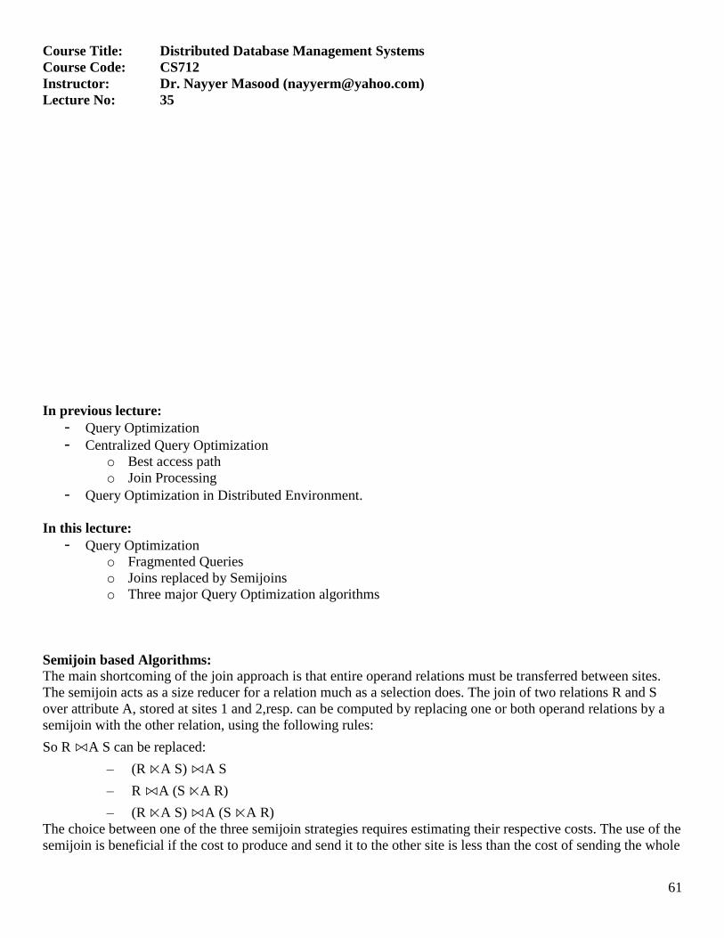
61


Course Code: CS712


Lecture No: 35



- Centralized Query Optimization

o Best access path

o Join Processing

- Query Optimization in Distributed Environment.

In this lecture:


o Fragmented Queries

o Joins replaced by Semijoins

o Three major Query Optimization algorithms

Semijoin based Algorithms:

The main shortcoming of the join approach is that entire operand relations must be transferred between sites.

The semijoin acts as a size reducer for a relation much as a selection does. The join of two relations R and S

over attribute A, stored at sites 1 and 2,resp. can be computed by replacing one or both operand relations by a

semijoin with the other relation, using the following rules:

So R ⋈A S can be replaced:

– (R ⋉A S) ⋈A S

– R ⋈A (S ⋉A R)

– (R ⋉A S) ⋈A (S ⋉A R)

The choice between one of the three semijoin strategies requires estimating their respective costs. The use of the

semijoin is beneficial if the cost to produce and send it to the other site is less than the cost of sending the whole

62

operand relation and of doing the actual join. To illustrate the potential benefit of the semijoin, let us compare

the costs of the two alternatives R ⋈A S verses (R ⋉A S) ⋈A S, assuming that size(R) < size (S).

The following program, using the semijoin operation:

1) A (S) site 1

2) Site1 computes R’ = R ⋉A S’

3) R’ site 2

4) Site2 computes R’ ⋈A S

For the sake of simplicity let us ignore the constant TMSG in the communication time assuming that the term

TTR*size(R) is much larger. We can then compare the two alternatives in terms of the amount of transmitted

data. The cost of the join-based algorithm is that of transferring relation R to site2. The cost of the semi-join

based algorithm is the cost of steps1 and 3 above. Therefore the semijoin approach is better if

Size(A(S)) + size(R ⋉A S) < size(R)

The semijoin approach is better if the semijoin acts as a sufficient reducer, if a few tuples of R participate in the

join. The join approach is better if almost all tuples of R participate in the join, because the semijoin approach

requires an additional transfer of a projection on the join attribute. The cost of projection step can be minimized

by encoding the result of the projection in bit arrays thereby reducing the cost of transferring the joined attribute

values. It is important to note that neither approach is systematically the best; they should be considered as

complementary.

The semijoin can be useful in reducing the size of the operand relations involved in multiple join queries. Query

optimization becomes more complex in these cases. Semijoin approach can be applied to each individual join,

consider an example:

Example:

Consider an example of a program to compute EMP ⋈ ASG ⋈ PROJ is

EMP’ ⋈ ASG’ ⋈ PROJ

where EMP’ = EMP ⋉ ASG and ASG’ = ASG ⋉ PROJ

We may further reduce the size of an operand relation by using more than one semioin. For example, EMP’ can

be replaced in the preceding program by EMP” derived as

EMP” = EMP ⋉ (ASG ⋉ PROJ)

Since if size (ASG ⋉ PROJ) <= size(ASG), we have size(EMP’’) <= size(EMP’). In this way EMP can be

reduced by the sequence of semijoins: EMP ⋉ASG ⋉ PROJ). Such a sequence of semijoins is called a semijoin

program for EMP. Similarly, semijoin programs can be found for any relation in a query. For example, PROJ

could be reduced by the semijoin program PROJ ⋉ (ASG ⋉ EMP). Not all of the relations involved in a query

need to be reduced; we can ignore those relations that are not involved in the final joins.

For a given relation, there exist several potential semijoin programs. The number of possibilities is in fact

exponential in the number of relations. But there is one optimal semijoin program called full reducer, which for

each relation R reduces R more than the others. The problem is to find the full reducer. A simple method is to

evaluate the size of all possible semijoin programs and to select the best one. The problems with the

enumerative method are twofold:

There is a class of queries, called cyclic queries that have cycles in their join graph and for which full reducers

can not be found

For other queries, called tree queries, full reduces exist, but the number of candidate semijoin programs is

exponential in the number of relations, which makes the enumerative approach NP-hard.

Example:

Consider a SQL query:

Select eName From EMP, ASG, PROJ Where

EMP.eNo = ASG.eNo and

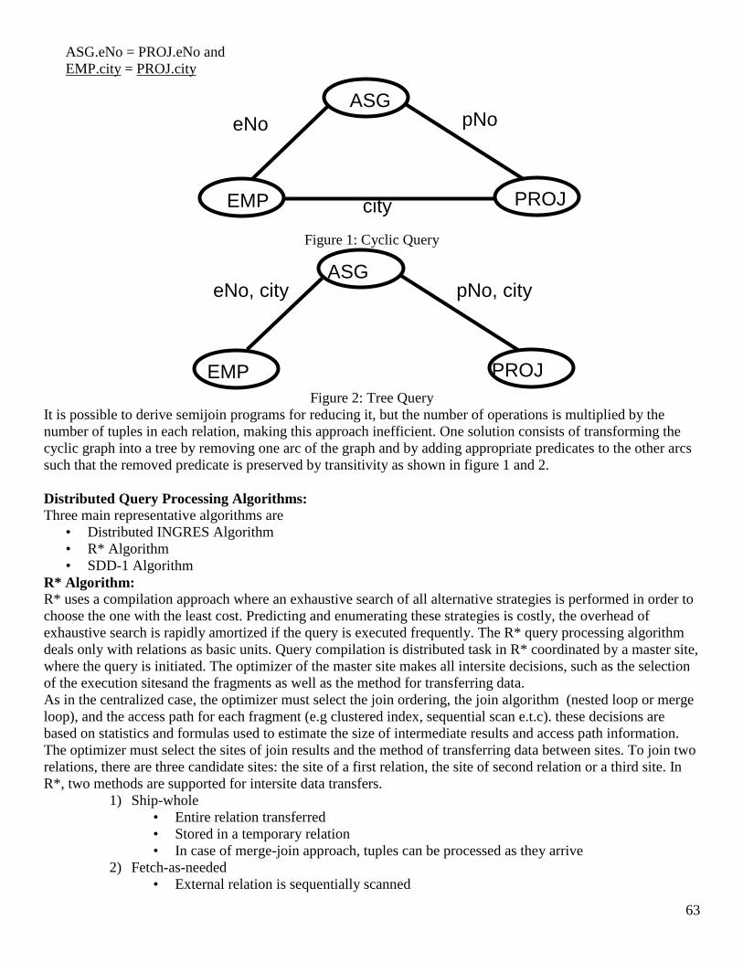
63

ASG.eNo = PROJ.eNo and

EMP.city = PROJ.city

Figure 1: Cyclic Query

Figure 2: Tree Query

It is possible to derive semijoin programs for reducing it, but the number of operations is multiplied by the

number of tuples in each relation, making this approach inefficient. One solution consists of transforming the

cyclic graph into a tree by removing one arc of the graph and by adding appropriate predicates to the other arcs

such that the removed predicate is preserved by transitivity as shown in figure 1 and 2.

Distributed Query Processing Algorithms:

Three main representative algorithms are

• Distributed INGRES Algorithm

• R* Algorithm

• SDD-1 Algorithm

R* Algorithm:

R* uses a compilation approach where an exhaustive search of all alternative strategies is performed in order to

choose the one with the least cost. Predicting and enumerating these strategies is costly, the overhead of

exhaustive search is rapidly amortized if the query is executed frequently. The R* query processing algorithm

deals only with relations as basic units. Query compilation is distributed task in R* coordinated by a master site,

where the query is initiated. The optimizer of the master site makes all intersite decisions, such as the selection

of the execution sitesand the fragments as well as the method for transferring data.

As in the centralized case, the optimizer must select the join ordering, the join algorithm (nested loop or merge

loop), and the access path for each fragment (e.g clustered index, sequential scan e.t.c). these decisions are

based on statistics and formulas used to estimate the size of intermediate results and access path information.

The optimizer must select the sites of join results and the method of transferring data between sites. To join two

relations, there are three candidate sites: the site of a first relation, the site of second relation or a third site. In

R*, two methods are supported for intersite data transfers.

1) Ship-whole

• Entire relation transferred

• Stored in a temporary relation

• In case of merge-join approach, tuples can be processed as they arrive

2) Fetch-as-needed

• External relation is sequentially scanned

EMP

ASG

PROJ

eNo pNo

city

EMP

ASG

PROJ

eNo, city pNo, city

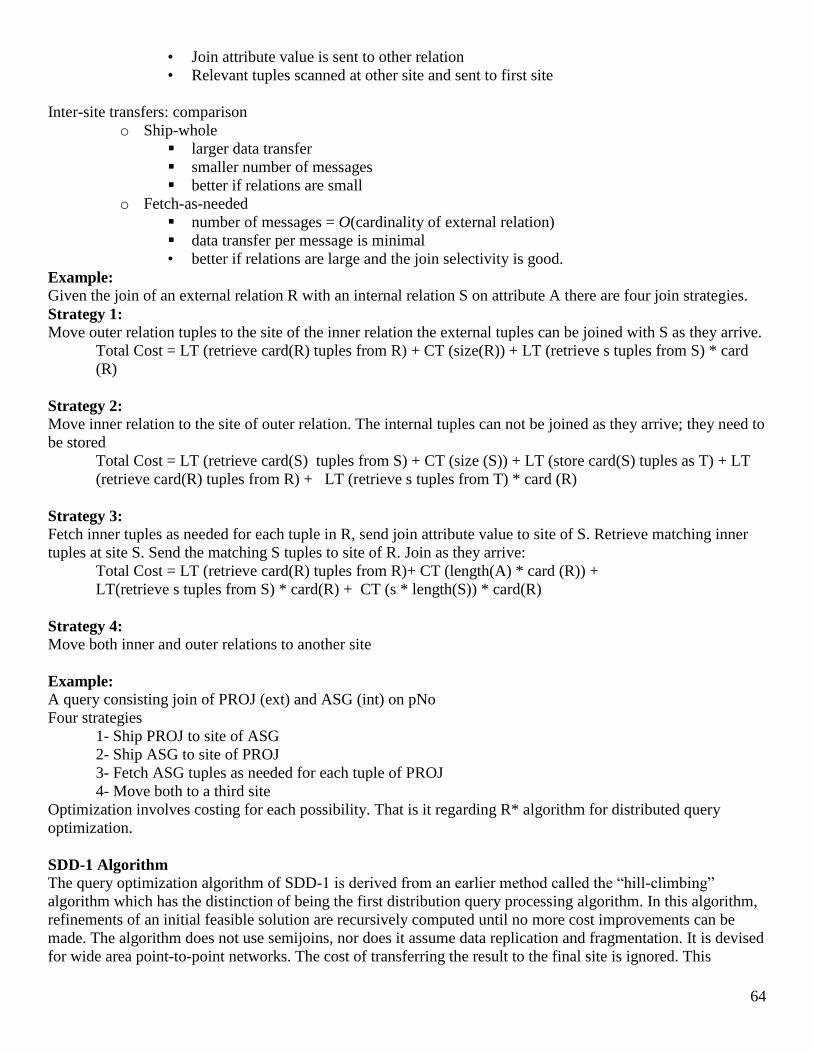
64

• Join attribute value is sent to other relation

• Relevant tuples scanned at other site and sent to first site

Inter-site transfers: comparison

o Ship-whole

larger data transfer

smaller number of messages

better if relations are small

o Fetch-as-needed

number of messages = O(cardinality of external relation)

data transfer per message is minimal

• better if relations are large and the join selectivity is good.

Example:

Given the join of an external relation R with an internal relation S on attribute A there are four join strategies.

Strategy 1:

Move outer relation tuples to the site of the inner relation the external tuples can be joined with S as they arrive.

Total Cost = LT (retrieve card(R) tuples from R) + CT (size(R)) + LT (retrieve s tuples from S) * card

(R)

Strategy 2:

Move inner relation to the site of outer relation. The internal tuples can not be joined as they arrive; they need to

be stored

Total Cost = LT (retrieve card(S) tuples from S) + CT (size (S)) + LT (store card(S) tuples as T) + LT

(retrieve card(R) tuples from R) + LT (retrieve s tuples from T) * card (R)

Strategy 3:

Fetch inner tuples as needed for each tuple in R, send join attribute value to site of S. Retrieve matching inner

tuples at site S. Send the matching S tuples to site of R. Join as they arrive:

Total Cost = LT (retrieve card(R) tuples from R)+ CT (length(A) * card (R)) +

LT(retrieve s tuples from S) * card(R) + CT (s * length(S)) * card(R)

Strategy 4:

Move both inner and outer relations to another site

Example:

A query consisting join of PROJ (ext) and ASG (int) on pNo

Four strategies

1- Ship PROJ to site of ASG

2- Ship ASG to site of PROJ

3- Fetch ASG tuples as needed for each tuple of PROJ

4- Move both to a third site

Optimization involves costing for each possibility. That is it regarding R* algorithm for distributed query

optimization.

SDD-1 Algorithm

The query optimization algorithm of SDD-1 is derived from an earlier method called the “hill-climbing”

algorithm which has the distinction of being the first distribution query processing algorithm. In this algorithm,

refinements of an initial feasible solution are recursively computed until no more cost improvements can be

made. The algorithm does not use semijoins, nor does it assume data replication and fragmentation. It is devised

for wide area point-to-point networks. The cost of transferring the result to the final site is ignored. This

65

algorithm is quite general in that it can minimize an arbitrary objective function, including the total time and

response time.

The hill climbing algorithm proceeds as follows.

1- The input to the algorithm includes the query graph, location of relations, and relation statistics.

2- Do the initial local processing

3- Select the initial best plan (ES0)

– Calculate cost of moving all relations to a single site

– Plan with the least cost is ES0

4- Split ES0 into ES1 and ES2

– ES1: Sending one of the relation to other site, relations joined there

– ES2:Sending the result back to site in ES0.

5- Replace ES0 with ES1 and ES2 when we should have

cost(ES1) + cost(local join) + cost (ES2) < cost (ES0)

6- Recursively apply step 3 and 4 on ES1 and ES2, until no improvement

Example

Find the salaries of engineers working on CAD/CAM project

• Involves EMP, PAY, PROJ and ASG

sal(PAY ⋈ title(EMP ⋈ eNo(ASG ⋈ pNo(pName = ‘CAD/CAM’ (PROJ)))))

Assume that Tmsg = 0 and TTR = 1. we ignore the local processing following which the database is

Relation Size Site

EMP

PAY

PROJ

ASG

8

4

1

10

1

2

3

4

Assume Length of a tuple is 1

So size(R) = card(R)

Considering only transfers costs Site 1

• PAY site 1 = 4

• PROJ site 1 = 1

• ASG site 1 = 10

• Total = 15

Cost for site 2 = 19



So site 4 is our ES0

Move all relations to site 4.

Summary

We have discussed Query Optimization, Fragmented Queries, Joins replaced by Semijoins. Three major Query

Optimization algorithms.

66


Course Code: CS712


Lecture No: 36



o Fragmented Queries

o Joins replaced by Semijoins

o Three major Query Optimization algorithms

Discussed R* Algorithm

Discussing SDD-1.

In this lecture:


o SDD-1 Algorithm continued

o Improvements in SDD-1 ALgo

o Overview of Query Processing

SDD-1 Algorithm continued:

From Previous Lecture

Example

Find the salaries of engineers working on CAD/CAM project

• Involves EMP, PAY, PROJ and ASG

sal(PAY ⋈ title(EMP ⋈ eNo(ASG ⋈ pNo(pName = ‘CAD/CAM’ (PROJ)))))

Assume that Tmsg = 0 and TTR = 1. We ignore the local processing following which the database is shown in

figure 1.

Relation Size Site

67

EMP

PAY

PROJ

ASG

8

4

1

10

1

2

3

4

Figure 1

Assume Length of a tuple is 1

So size(R) = card(R)

Considering only data transfers the initial feasible solution is to choose sie4 as the result site, producing the

schedule.

Site 4

–PAY site 4 = 4

–PROJ site 4 = 1

–EMP site 4 = 8

Total = 13

The minimum cost option, so ES0

One possible way of splitting this schedule (call it ES’) is the following:

–ES1: EMP site 2

–ES2: (EMP ⋈ PAY) site 4

–ES3: PROJ site 4

–Cost = 8 + 8 + 1 = 17

Other possibilities suggest that ES0 should not be split

Problems:

•The hill-climbing algorithm is in the class of greedy algorithms, which start with an initial feasible solution

and iteratively improve it. The main problem is that strategies with higher cost, which could nevertheless

produce better overall benefits, are ignored. If the optimal schedule has a high initial cost, it won't find it, An

optimum solution with multiple sites is ignored, for example.

A better schedule is

PROJ → Site 4

ASG' = (PROJ ⋈ ASG) → Site 1

(ASG' ⋈ EMP) → Site 2

Total cost = 1 + 2 + 2 = 5

The hill climbing algorithm has been substantially improved in SDD-1 in a number of ways. The improved

version makes extensive use of semijoins. The objective function is expressed in terms of total communication

time. Finally, the algorithm uses statistics on the database, called database profiles, where a profile is associated

with a relation. The improved version also selects an initial feasible solution that is iteratively refined.

Furthermore, a postoptimization step is added to improve the total time of the solution selected. The main step

of the algorithm consists of determining and ordering beneficial semijoins, that is semijoins whose cost is less

than their benefit. The cost of semijoin is that of transferring the semijoin attributes A.

Cost(R ⋉ A S) = TMSG + TTR * size(A(S))

68

While its benefit is the cost of transferring irrelevant tuples of R (which is avoided by the semijoin):

Benefit(R ⋉ A S) = (1-SFSJ(S.A)) *size(R) * TTR

Phases of SDD-1:

There are four phases:

1. Initialization

2. Selection of beneficial semijoins

3. Assembly site selection

4. Postoptimization

The initialization phase generates a set of beneficial smijoins: BS= {SJ1, SJ2, …, SJk) and an execution strategy

that includes only local processing. The next phase selects the beneficial semijoins from BS by iteratively

choosing the most beneficial semijoin, SJi and modeling the database statistics and BS accordingly. The next

phase computes the assembly site by evaluating, for each candidate site, the cost of transferring to it all the

required data and taking the one with the least cost. A postoptimization phase permits the removal from the

execution strategy of those semijoins that affect only relations stored at assembly site.

Example:

Let us consider the following query as shown in figure 2:

SELECT * FROM

EMP, ASG, PROJ WHERE

EMP.eNo = ASG.eNo AND

ASG.pNo = PROJ.pNo

Relation Card Tuple size Rel. size

EMP

ASG

PROJ

30

100

50

50

30

40

1500

3000

2000

Attribute SFSJ Size(attrib)

EMP.eNo

ASG.eNo

ASG.pNo

PROJ.pNo

0.3

1.0

1.0

0.4

120

400

400

200

Figure 2: Example Query and Statistics

EMP ⋈ ASG ⋈ PROJ

–EMP ⋉ ASG

–ASG ⋉ EMP

–ASG ⋉ PROJ

EMP ASG PROJ

eNo pNo

Site 1 Site 3 Site 2

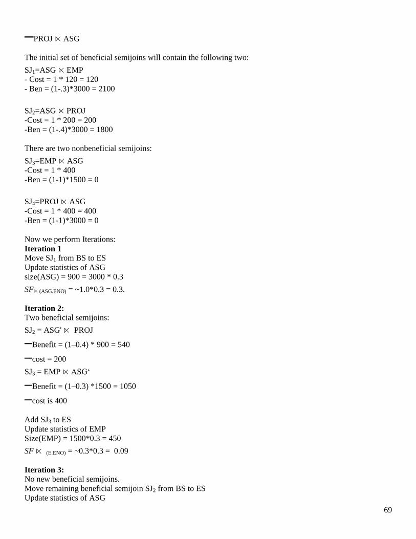
69

–PROJ ⋉ ASG

The initial set of beneficial semijoins will contain the following two:

SJ1=ASG ⋉ EMP

- Cost = 1 * 120 = 120

- Ben = (1-.3)*3000 = 2100

SJ2=ASG ⋉ PROJ

-Cost = 1 * 200 = 200

-Ben = (1-.4)*3000 = 1800

There are two nonbeneficial semijoins:

SJ3=EMP ⋉ ASG

-Cost = 1 * 400

-Ben = (1-1)*1500 = 0

SJ4=PROJ ⋉ ASG

-Cost = 1 * 400 = 400

-Ben = (1-1)*3000 = 0

Now we perform Iterations:

Iteration 1

Move SJ1 from BS to ES

Update statistics of ASG

size(ASG) = 900 = 3000 * 0.3

SF⋉ (ASG.ENO) = ~1.0*0.3 = 0.3.

Iteration 2:

Two beneficial semijoins:

SJ2 = ASG' ⋉ PROJ

–Benefit = (1–0.4) * 900 = 540

–cost = 200

SJ3 = EMP ⋉ ASG‘

–Benefit = (1–0.3) *1500 = 1050

–cost is 400

Add SJ3 to ES

Update statistics of EMP

Size(EMP) = 1500*0.3 = 450

SF ⋉ (E.ENO) = ~0.3*0.3 = 0.09

Iteration 3:

No new beneficial semijoins.

Move remaining beneficial semijoin SJ2 from BS to ES

Update statistics of ASG

70

Size(ASG) = 900*0.4 = 360

Assembly Site Selection: The site where the largest amount of data resides

Example:

Amount of data stored at:

–Site 1: 450

–Site 2: 360

–Site 3: 2000 (Assembly Site)

For each Ri at the assembly site, find the semijoins of the type Ri ⋉ Rj where the total cost of ES without this

semijoin is smaller than the cost with it and remove the semijoin from ES. No semijoins are removed in our

example

Permute the order of semijoins if doing so would improve the total cost of ES

Final ES = {(ASG ⋉ EMP), (ASG’ ⋉ PROJ), (EMP ⋉ ASG’)}, Execution site = 3

Final Strategy: Send (ASG ⋉ EMP) ⋉ PROJ and EMP ⋉ ASG’ to Site 3

Summary of QP

QP involves

–Accepting User Query (SQL)

–Establishing exec strategy

–Query optimization

QP objective is to reduce the cost function: involves I/O time, CPU time and communication time

Layers of QP

1. Query Decomposition

2. Data Localization

3. Global Query Optimization

4. Local Query Optimization.

1- Query Decomposition

Transforms an SQL query to Relational Algebra one on the global relations

Four phases:

1.1 Normalization: Rewrites in a proper format

1.2 Analysis: checks type and semantically incorrect ones

1.3 Elimination of Redundancy

1.4 Rewriting: in relational algebra-

2- Data Localization

Input is a query tree

Localizes the query data using the data distribution information from global schema: two steps.

2.1 Simplification: replaces the relation names with the fragments names

2.2 Fragment query is simplified and restructured to produce a good one-

3- Global Query Optimization:

Finding the best ordering of operations in fragmented query including comm. cost

Extension of Centralized QO

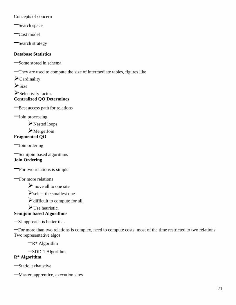
71

Concepts of concern

–Search space

–Cost model

–Search strategy

Database Statistics

–Some stored in schema

–They are used to compute the size of intermediate tables, figures like

Cardinality

Size

Selectivity factor.

Centralized QO Determines

–Best access path for relations

–Join processing

Nested loops

Merge Join

Fragmented QO

–Join ordering

–Semijoin based algorithms

Join Ordering

–For two relations is simple

–For more relations

move all to one site

select the smallest one

difficult to compute for all

Use heuristic.

Semijoin based Algorithms

–SJ approach is better if…

–For more than two relations is complex, need to compute costs, most of the time restricted to two relations

Two representative algos

–R* Algorithm

–SDD-1 Algorithm

R* Algorithm

–Static, exhaustive

–Master, apprentice, execution sites

72

–Ship-whole, fetch-as-needed

–Adopts four strategies, computes cost for each and adopts the best one.

SDD-1 Algorithm

–Input: Query Graph, DB Statistics, location of relations

–Select an initial plan ES0, one that gives minimum transfer cost

–Improve ES0 iteratively, unless no further improvement.

–See the beneficial SJs, where benefit is more than the cost, move them to BS

–Move best SJ from BS to ES

–Adjust the statistics based on the selected SJ

–Iteratively move all beneficial SJ to ES.

–Pass through postoptimization phase

–Select the execution site, one that contains maximum data, move the selected SJs to that site.


Course Code: CS712


Lecture No: 37

73

In today’s lecture:

- Parallel Database Systems

o Basics of Parallel Processing

o Parallel Database Systems

References for the topic

Crichlow, J. M.,”An Introduction to Distributed and Parallel Computing” second ed., PHI

Mahapatra,T., Mishra, S., “Oracle Parallel Processing”, O’Relly Online Catalogue

Parallel Processing:

Introduction:

Computer programs generally execute sequentially, reasons are:

– Single CPU

– Programming language support

– Programmer familiarity

– Logic of program is sequential

Uni-processor multi-programming systems allow concurrent processing through context switching. However,

CPU runs one instruction at a time. Parallel processing involves taking a large task, dividing it into several

smaller tasks, and then working on each of those smaller tasks simultaneously. This divide-n-conquer strategy

performs larger task in less time.

Requirements for parallel processing:

• Computer Hardware

• An operating system capable of managing multiple processors

• Application software

Why parallel processing:

Some Applications need computing power of parallel system

• image processing

• large-scale simulation

• Weather forecasting etc.

Advantages:

Parallel processing has following advantages:

• More fault tolerance

• Increases throughput

• Better price/performance

Costs involved:

• Synchronization cost has to be kept minimum

• Administering is difficult

Many computer programs can be broken into distinct parallel procedures, like

for i = 1 to n

c(i) = a(i) *a(i) + sqrt(a(i))

Where c and a are array

74

Square and square root can be done in parallel in parallel processing. So the execution speed increases. Systems

allow moving away from strict serial execution to parallel processing. There are different architectures in

parallel processing:

• Pipeline machines

• Multicomputers

• Multiprocessors

• Massively parallel architecture

Pipeline and Vector Processors

Pipeline processors permit overlapping of instructions. This is also called producer-consumer. An instruction

divided into a number of distinct stages, each allocated to distinct processor. Like, steps may be

1. Fetch instruction

2. Decode it

3. Calculate effective address of operands

4. Get operands

5. Execute operations

6. Store result

For example, there are six processors. First processor gives the output to second and starts the next instruction

first step. So in this way six instructions run in pipeline manner.

Determination of operation involved here. If operation is same on large amount of data, so the step fetch and

decode will skip and just perform other four steps so execution will be fast. This process is called vector

processing.

Multicomputer Systems

Multiple computers linked through a network in a small area. They are loosely coupled systems and they are

also called MIMD (multiple instructions multiple data) machines. Different instructions execute on different

machines. They are physical connected via bus or channel and allows parallel stream transmission of data. In

multicomputer systems data transmission speed will be fast, low transmission errors because of less distance

and skew is immaterial. Skew means sub tasks perform in parallel so there is a time variation exists.

Multicomputer can be used to distribute processing by type e.g. if there is a task then this involve number of

activities and each computer assign a one activity e.g. one is used for input/output and one for report and so on.

These computers must interact with each other. One possibility for load balancing establishes a setup of

Master/Slave. Second setup is of Multiple Master/Slave. Third is Peer to peer, anyone initiates a job, interested

processors bid.

Summary

We have discussed the basics of parallel processing and parallel database systems. Parallel database system is

the combination of parallel processing and database concepts.

75


Course Code: CS712


Lecture No: 38

In the previous lecture:

- Sequential Execution

- Parallel Execution

- Non-Sequential setups

o Pipeline and Vector Processor

o Multicomputer Systems


- Parallel Processing basics

o Multiprocessor Systems

o Associative Processors

o Array Processors

- Entry to Parallel Database Systems

Multiprocessor Systems

Multiprocessing is the use of two or more central processing units (CPUs) within a single computer system as

shown in figure 1. One computer with a global RAM shared by many processors. All processors are tightly

coupled. In multiprocessor, thousands of processor is controlled by single operating system. Each processor

accessing the same job queue. Synchronization between them is required. Contention for resources may be

occurring. Interprocessor communication is also required. Processors may be allocated buffer areas in memory

for interProcessor information transfer.

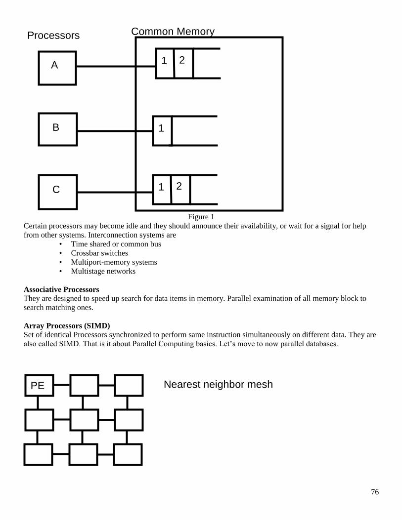
76

Figure 1

Certain processors may become idle and they should announce their availability, or wait for a signal for help

from other systems. Interconnection systems are

• Time shared or common bus

• Crossbar switches

• Multiport-memory systems

• Multistage networks

Associative Processors

They are designed to speed up search for data items in memory. Parallel examination of all memory block to

search matching ones.

Array Processors (SIMD)

Set of identical Processors synchronized to perform same instruction simultaneously on different data. They are

also called SIMD. That is it about Parallel Computing basics. Let’s move to now parallel databases.

Processors

A

B

C

1 2

1

1 2

Common Memory

PE Nearest neighbor mesh

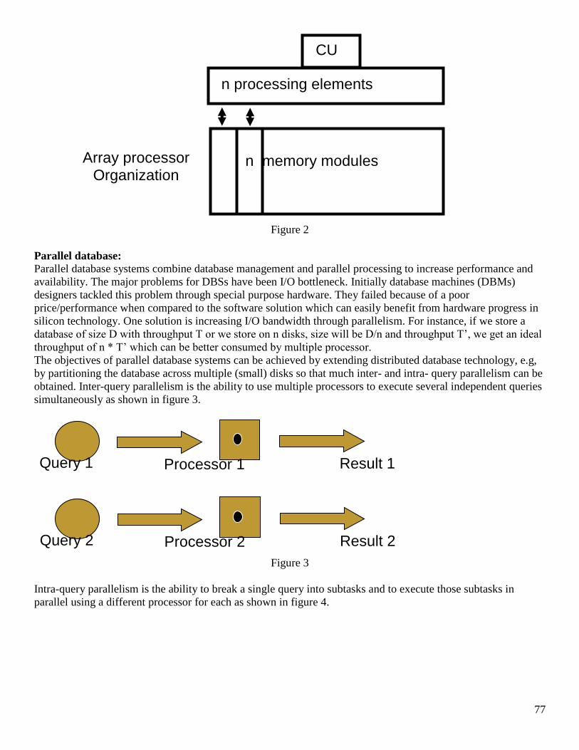
77

Figure 2

Parallel database:

Parallel database systems combine database management and parallel processing to increase performance and

availability. The major problems for DBSs have been I/O bottleneck. Initially database machines (DBMs)

designers tackled this problem through special purpose hardware. They failed because of a poor

price/performance when compared to the software solution which can easily benefit from hardware progress in

silicon technology. One solution is increasing I/O bandwidth through parallelism. For instance, if we store a

database of size D with throughput T or we store on n disks, size will be D/n and throughput T’, we get an ideal

throughput of n * T’ which can be better consumed by multiple processor.

The objectives of parallel database systems can be achieved by extending distributed database technology, e.g,

by partitioning the database across multiple (small) disks so that much inter- and intra- query parallelism can be

obtained. Inter-query parallelism is the ability to use multiple processors to execute several independent queries

simultaneously as shown in figure 3.

Figure 3

Intra-query parallelism is the ability to break a single query into subtasks and to execute those subtasks in

parallel using a different processor for each as shown in figure 4.

CU

n processing elements

n memory modules Array processor Organization

Query 1 Processor 1 Result 1

Query 2 Processor 2 Result 2

78

Figure 4

A parallel database system can be loosely defined as a DBMS implemented on a tightly coupled multiprocessor.

A Parallel database system acts as a DB server to multiple application servers in now client-server organization

in computer networks. It supports

– DB functions

– C/S interface

– Also general purpose computing

Advantages A parallel database system should provide the following advantages:

1) High Performance: This can be obtained through several complementary solutions: DB-Oriented Operating System support,

parallelism, optimization, and load balancing. Having the operating system constrained and aware of the

specific database requirements (e.g. buffer management) simplifies the implementation of low-level

database functions and therefore decreases their cost. Parallelism can increase throughput, using inter-query

parallelism and decrease transaction response times, using intra query parallelism. Load balancing is the

ability of system to divide a given workload equally among all processors.

2) High availability Because a parallel database system consists of many similar components, it can exploit data replication to

increase database availability. In a high parallel system with many small disks, the probability of a disk

failure at any time can be higher. Its is essential that a disk failure does not imbalance the load, e.g. by

doubling the load on the available copy. Solutions to this problem require partitioning copies in such a way

that they can also be accessed in parallel.

3) Extensibility In a parallel environment, accommodating increasing database sizes or increasing performance demands

should be easier. Extensibility is the ability of smooth expansion of system by adding processing and

storage power to the system. The parallel database system should demonstrate two advantages

– Linear scaleup

– Linear speedup

Extending the system should require minimum reorganization of existing database.

Architecture of a parallel database system

Assuming client server architecture, the functions supported by a parallel database system can be divided into

three subsystems much like in a typical RDBMS. Depending on the architecture, processor can support all (or a

subset) of these subsystems. Figure 5 shows the architecture:

Processors

Results

Query

Subtask1

Subtask2 Merging

Final Result

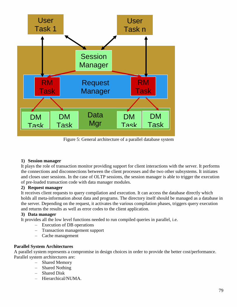
79

Figure 5: General architecture of a parallel database system

1) Session manager

It plays the role of transaction monitor providing support for client interactions with the server. It performs

the connections and disconnections between the client processes and the two other subsystems. It initiates

and closes user sessions. In the case of OLTP sessions, the session manager is able to trigger the execution

of pre-loaded transaction code with data manager modules.

2) Request manager

It receives client requests to query compilation and execution. It can access the database directly which

holds all meta-information about data and programs. The directory itself should be managed as a database in

the server. Depending on the request, it activates the various compilation phases, triggers query execution

and returns the results as well as error codes to the client application.

3) Data manager

It provides all the low level functions needed to run compiled queries in parallel, i.e.

– Execution of DB operations

– Transaction management support

– Cache management

Parallel System Architectures

A parallel system represents a compromise in design choices in order to provide the better cost/performance.

Parallel system architectures are:

– Shared Memory

– Shared Nothing

– Shared Disk

– Hierarchical/NUMA.

Session Manager

Data Mgr

Request Manager

User Task n

User Task 1

RM Task

1

RM Task

n

DM Task 12

DM Task

DM Task n2

DM Task

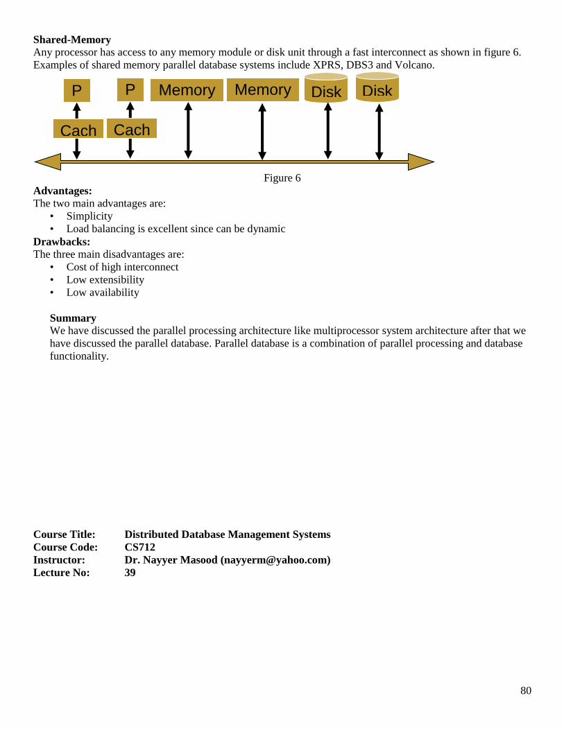
80

Shared-Memory

Any processor has access to any memory module or disk unit through a fast interconnect as shown in figure 6.

Examples of shared memory parallel database systems include XPRS, DBS3 and Volcano.

Figure 6

Advantages: The two main advantages are:

• Simplicity

• Load balancing is excellent since can be dynamic

Drawbacks:

The three main disadvantages are:

• Cost of high interconnect

• Low extensibility

• Low availability

Summary

We have discussed the parallel processing architecture like multiprocessor system architecture after that we

have discussed the parallel database. Parallel database is a combination of parallel processing and database

functionality.


Course Code: CS712


Lecture No: 39

P1

Cache

P2

Cache

Memory 1

Memory 2

Disk 2

Disk 1

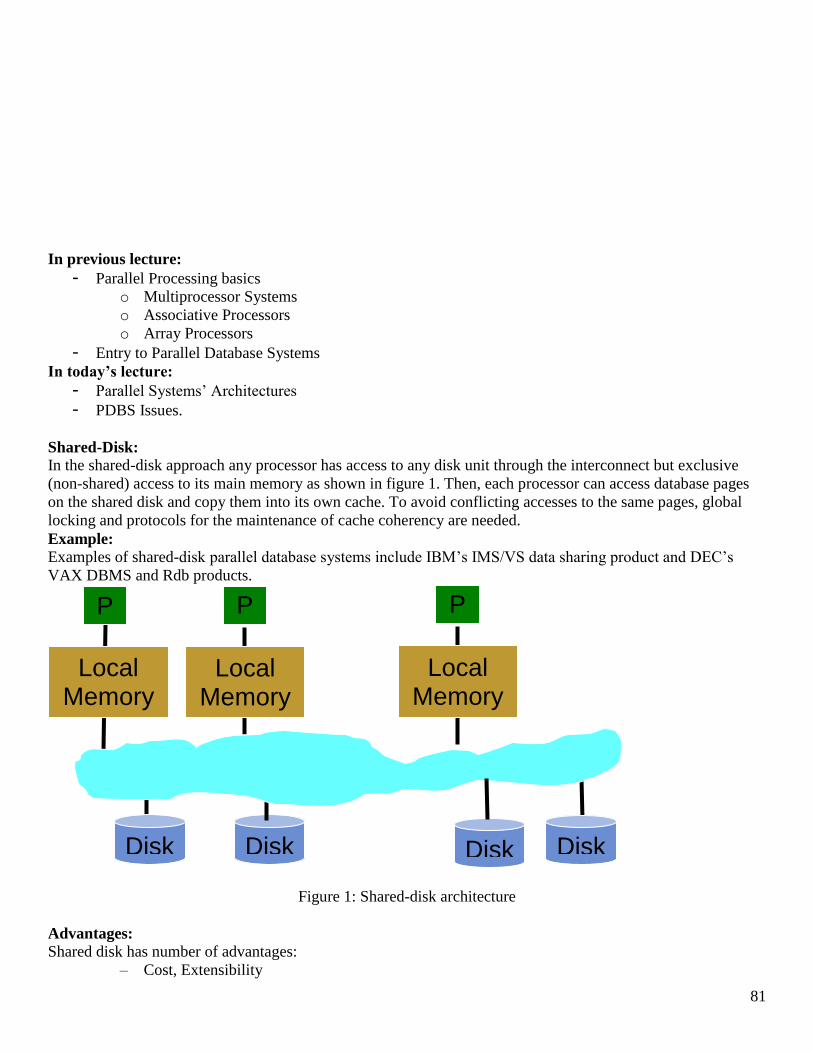
81


- Parallel Processing basics

o Multiprocessor Systems

o Associative Processors

o Array Processors

- Entry to Parallel Database Systems


- Parallel Systems’ Architectures

- PDBS Issues.

Shared-Disk:

In the shared-disk approach any processor has access to any disk unit through the interconnect but exclusive

(non-shared) access to its main memory as shown in figure 1. Then, each processor can access database pages

on the shared disk and copy them into its own cache. To avoid conflicting accesses to the same pages, global

locking and protocols for the maintenance of cache coherency are needed.

Example:

Examples of shared-disk parallel database systems include IBM’s IMS/VS data sharing product and DEC’s

VAX DBMS and Rdb products.

Figure 1: Shared-disk architecture

Advantages:

Shared disk has number of advantages:

– Cost, Extensibility

P1

P2

Local Memory

Local Memory

Disk Disk

Pn

Local Memory

Disk Disk

82

– Easy migration from Uniprocessor systems

– Load balancing

Demerits:

Shared disk suffers from:

– Higher complexity

– Potential performance problems

Shared-Nothing:

In shares-nothing approach each processor has exclusive access to its main memory and disk unit(s) as shown in

figure 2. Then each node can be viewed as a local site(with its own database and software) in a distributed

database system. Therefore, most solutions designed for distributed database such as database fragmentation,

distributed transaction management and distributed query processing may be reused.

Examples:

Examples of shared-nothing parallel database systems include he Teradata’s DBC and Tandem’s NonStopSQL

products as well as number of prototypes such as BUBBA, EDS, GAMMA and so on.

Figure 2: Shared-nothing architecture

Advantages: Shared-nothing has following advantages:

– Cost

– Availability and extensibility

Drawbacks:

Shared-nothing has following disadvantages:

– More complex than shared memory

– Difficult load balancing

Hierarchical Architecture

Hierarchical architecture (also called cluster architecture), is a combination of shared- noting and shared-

memory. The idea is to build a shared-nothing machine whose nodes are shared-memory.

Advantage:

The advantage of hierarchical architecture is:

Combines the benefits of both shared memory and shared-nothing

NUMA Architectures

• Non-uniform memory access

• To provide benefits of shared-memory model in a scalable parallel architecture

Two classes of NUMA

P1

P2

Local Memory

Local Memory

Disk Disk

Pn

Local Memory

Disk

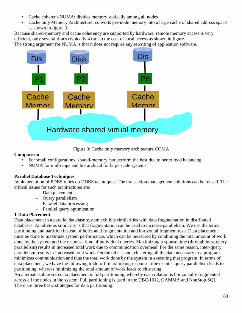
83

• Cache coherent-NUMA: divides memory statically among all nodes

• Cache only Memory Architecture: converts per-node memory into a large cache of shared address space

as shown in figure 3.

Because shared-memory and cache coherency are supported by hardware, remote memory access is very

efficient, only several times (typically 4 times) the cost of local access as shown in figure.

The strong argument for NUMA is that it does not require any rewriting of application software.

Figure 3: Cache only memory architecture COMA

Comparison

• For small configurations, shared-memory can perform the best due to better load balancing

• NUMA for mid-range and hierarchical for large scale systems

Parallel Database Techniques

Implementation of PDBS relies on DDBS techniques. The transaction management solutions can be reused. The

critical issues for such architectures are:

– Data placement

– Query parallelism

– Parallel data processing

– Parallel query optimization

1-Data Placement

Data placement in a parallel database system exhibits similarities with data fragmentation in distributed

databases. An obvious similarity is that fragmentation can be used to increase parallelism. We use the terms

partitioning and partition instead of horizontal fragmentation and horizontal fragment resp. Data placement

must be done to maximize system performance, which can be measured by combining the total amount of work

done by the system and the response time of individual queries. Maximizing response time (through intra-query

parallelism) results in increased total work due to communication overhead. For the same reason, inter-query

parallelism results in I ncreased total work. On the other hand, clustering all the data necessary to a program

minimizes communication and thus the total work done by the system in executing that program. In terms of

data placement, we have the following trade-off: maximizing response time or inter-query parallelism leads to

partitioning, whereas minimizing the total amount of work leads to clustering.

An alternate solution to data placement is full partitioning, whereby each relation is horizontally fragmented

across all the nodes in the system. Full partitioning is used in the DBC/1012, GAMMA and NonStop SQL.

There are three basic strategies for data partitioning:

P1 P2

Cache Memor

Cache Memory

Disk Disk

Pn

Cache Memor

Dis

Hardware shared virtual memory

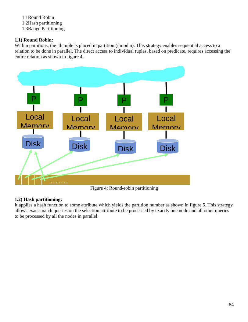
84

1.1Round Robin

1.2Hash partitioning

1.3Range Partitioning

1.1) Round Robin: With n partitions, the ith tuple is placed in partition (i mod n). This strategy enables sequential access to a

relation to be done in parallel. The direct access to individual tuples, based on predicate, requires accessing the

entire relation as shown in figure 4.

Figure 4: Round-robin partitioning

1.2) Hash partitioning:

It applies a hash function to some attribute which yields the partition number as shown in figure 5. This strategy

allows exact-match queries on the selection attribute to be processed by exactly one node and all other queries

to be processed by all the nodes in parallel.

P P

Local Memory

Local Memory

Disk Disk

P

Local Memory

Disk

P

Local Memory

Disk

…….

85

Figure 5: Hash partitioning

1.3) Range Partitioning: It distributes tuples based on value intervals of some attribute as shown in figure 6. It is suitable for exact match

and range queries. Range partition can result in high variation in partition size.

Figure 6: Range partitioning

The performance of full partitioning is compared to that of clustering the relations on single disk. The results

indicate that for a wide variety of multi-user workloads, partitioning is consistently better. Clustering may

dominate in processing complex queries (e.g. joins). A solution to data placement by variable partitioning is

P P

Local Memory

Local Memory

Disk Disk

P

Local Memory

Disk

P

Local Memory

Disk

…….

P P

Local Memory

Local Memory

H-M A-G

P

Local Memory

N-R

P

Local Memory

S-Z

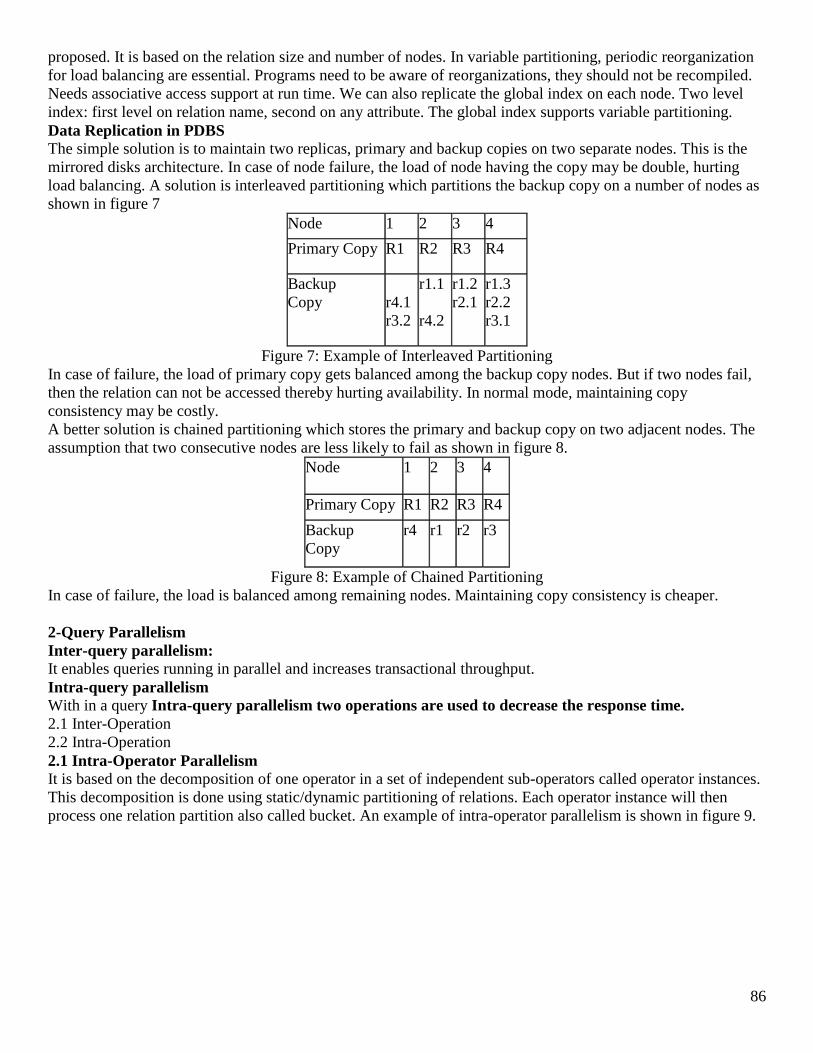
86

proposed. It is based on the relation size and number of nodes. In variable partitioning, periodic reorganization

for load balancing are essential. Programs need to be aware of reorganizations, they should not be recompiled.

Needs associative access support at run time. We can also replicate the global index on each node. Two level

index: first level on relation name, second on any attribute. The global index supports variable partitioning.

Data Replication in PDBS

The simple solution is to maintain two replicas, primary and backup copies on two separate nodes. This is the

mirrored disks architecture. In case of node failure, the load of node having the copy may be double, hurting

load balancing. A solution is interleaved partitioning which partitions the backup copy on a number of nodes as

shown in figure 7

Node 1 2 3 4

Primary Copy R1 R2 R3 R4

Backup

Copy

r4.1

r3.2

r1.1

r4.2

r1.2

r2.1

r1.3

r2.2

r3.1

Figure 7: Example of Interleaved Partitioning

In case of failure, the load of primary copy gets balanced among the backup copy nodes. But if two nodes fail,

then the relation can not be accessed thereby hurting availability. In normal mode, maintaining copy

consistency may be costly.

A better solution is chained partitioning which stores the primary and backup copy on two adjacent nodes. The

assumption that two consecutive nodes are less likely to fail as shown in figure 8.

Node 1 2 3 4

Primary Copy R1 R2 R3 R4

Backup

Copy

r4 r1 r2 r3

Figure 8: Example of Chained Partitioning

In case of failure, the load is balanced among remaining nodes. Maintaining copy consistency is cheaper.

2-Query Parallelism

Inter-query parallelism: It enables queries running in parallel and increases transactional throughput.

Intra-query parallelism

With in a query Intra-query parallelism two operations are used to decrease the response time.

2.1 Inter-Operation

2.2 Intra-Operation

2.1 Intra-Operator Parallelism

It is based on the decomposition of one operator in a set of independent sub-operators called operator instances.

This decomposition is done using static/dynamic partitioning of relations. Each operator instance will then

process one relation partition also called bucket. An example of intra-operator parallelism is shown in figure 9.

87

Figure 9: Intra-operator parallelism

Select query: can be decomposed directly. If the relation is partitioned on select predicate attribute, query may

be executed on some partitions not all. For the Join operator, it is more complex to decompose the operator. One

approach is to join each partition of R with S, but such a join will be inefficient. A more efficient way is to use

partitioning properties.

2.2) Inter-Operator Parallelism

Two forms of Inter-operator parallelism can be exploited.

Pipeline parallelism

Independent parallelism

Pipeline parallelism: several operators with a producer-consumer link are executed in parallel.

Independent parallelism: is achieved when there in no dependency between the operators executed in parallel.

An example of inter-operator parallelism is shown in figure 10.

Figure 10: Inter-operator parallelism

Summary

We have discussed the query parallelism. In query parallel parallelism there are two possibilities: intra-operator

parallelism and inter-operator parallelism. In intra-operator parallelism one query has operators and they will

work in parallel. In inter-operator parallelism work will be done through pipeline and independent parallelism.

Op

R

Op

R1

Op

R2

Op

R3

Op

R4

Join

Select Select

88


Course Code: CS712


Lecture No: 40


- Data Placement

- Parallel Query Processing


- Parallel Data Processing

- Parallel Query Optimization

3-Parallel Data Processing:

Partitioned data placement is the basis for the parallel execution of database queries. Given a portioned data

placement, an important issue is the design parallel algorithms for an efficient processing of database operators

(i.e relational algebra operators) and database queries which combine multiple operators. The issue is difficult

because a good trade-off between parallelism and communication cost must be reached. Parallel algorithms for

relational algebra operators are the building blocks necessary for parallel query processing. Parallel data

processing should exploit intra-operation parallelism. The distributed join algorithms designed for high speed

networks. Three basic parallel join algorithms for partitioned databases:

– Parallel Nested Loop (PNL)

– Parallel Associative Join (PAJ)

– Parallel Hash Join (PHJ)

Assumptions

• R and S are partitioned over m and n nodes

• m and n nodes are distinct

• Nodes are called R-nodes and S-nodes

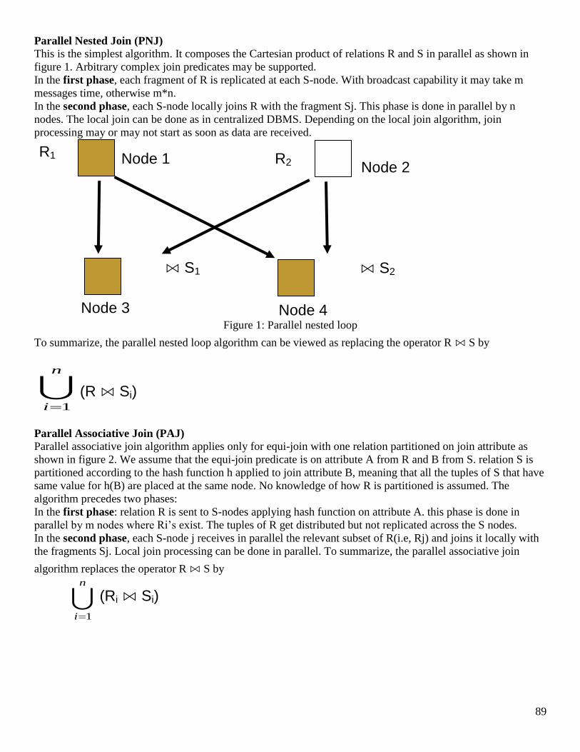
89

Parallel Nested Join (PNJ)

This is the simplest algorithm. It composes the Cartesian product of relations R and S in parallel as shown in

figure 1. Arbitrary complex join predicates may be supported.

In the first phase, each fragment of R is replicated at each S-node. With broadcast capability it may take m

messages time, otherwise m*n.

In the second phase, each S-node locally joins R with the fragment Sj. This phase is done in parallel by n

nodes. The local join can be done as in centralized DBMS. Depending on the local join algorithm, join

processing may or may not start as soon as data are received.

Figure 1: Parallel nested loop

To summarize, the parallel nested loop algorithm can be viewed as replacing the operator R ⋈ S by

Parallel Associative Join (PAJ)

Parallel associative join algorithm applies only for equi-join with one relation partitioned on join attribute as

shown in figure 2. We assume that the equi-join predicate is on attribute A from R and B from S. relation S is

partitioned according to the hash function h applied to join attribute B, meaning that all the tuples of S that have

same value for h(B) are placed at the same node. No knowledge of how R is partitioned is assumed. The

algorithm precedes two phases:

In the first phase: relation R is sent to S-nodes applying hash function on attribute A. this phase is done in

parallel by m nodes where Ri’s exist. The tuples of R get distributed but not replicated across the S nodes.

In the second phase, each S-node j receives in parallel the relevant subset of R(i.e, Rj) and joins it locally with

the fragments Sj. Local join processing can be done in parallel. To summarize, the parallel associative join

algorithm replaces the operator R ⋈ S by

n

i 1

(R ⋈ Si)

⋈ S1 ⋈ S2

Node 1 Node 2

R2 R1

Node 3 Node 4

n

i 1

(Ri ⋈ Si)

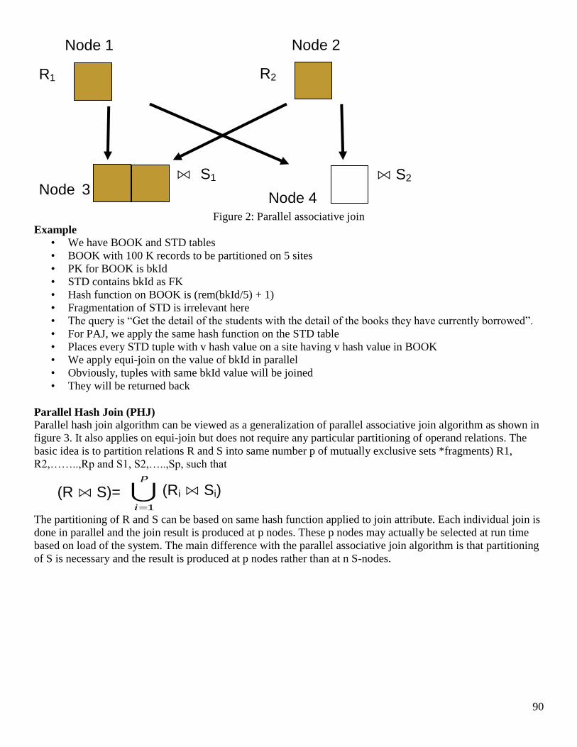
90

Figure 2: Parallel associative join

Example

• We have BOOK and STD tables

• BOOK with 100 K records to be partitioned on 5 sites

• PK for BOOK is bkId

• STD contains bkId as FK

• Hash function on BOOK is (rem(bkId/5) + 1)

• Fragmentation of STD is irrelevant here

• The query is “Get the detail of the students with the detail of the books they have currently borrowed”.

• For PAJ, we apply the same hash function on the STD table

• Places every STD tuple with v hash value on a site having v hash value in BOOK

• We apply equi-join on the value of bkId in parallel

• Obviously, tuples with same bkId value will be joined

• They will be returned back

Parallel Hash Join (PHJ)

Parallel hash join algorithm can be viewed as a generalization of parallel associative join algorithm as shown in

figure 3. It also applies on equi-join but does not require any particular partitioning of operand relations. The

basic idea is to partition relations R and S into same number p of mutually exclusive sets *fragments) R1,

R2,……..,Rp and S1, S2,…..,Sp, such that

The partitioning of R and S can be based on same hash function applied to join attribute. Each individual join is

done in parallel and the join result is produced at p nodes. These p nodes may actually be selected at run time

based on load of the system. The main difference with the parallel associative join algorithm is that partitioning

of S is necessary and the result is produced at p nodes rather than at n S-nodes.

p

i 1

(Ri ⋈ Si) (R ⋈ S)=

⋈ S1 ⋈ S2

Node 1 Node 2

R2 R1

Node 3 Node 4

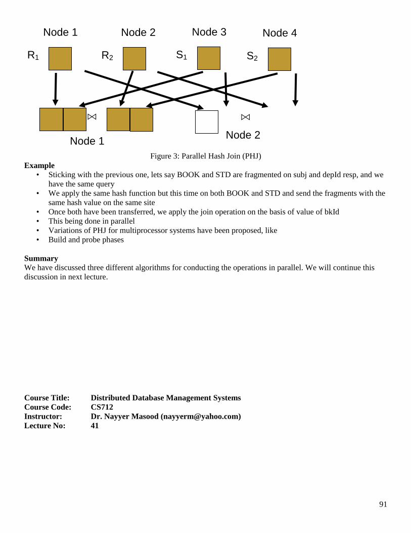
91

Figure 3: Parallel Hash Join (PHJ)

Example

• Sticking with the previous one, lets say BOOK and STD are fragmented on subj and depId resp, and we

have the same query

• We apply the same hash function but this time on both BOOK and STD and send the fragments with the

same hash value on the same site

• Once both have been transferred, we apply the join operation on the basis of value of bkId

• This being done in parallel

• Variations of PHJ for multiprocessor systems have been proposed, like

• Build and probe phases

Summary

We have discussed three different algorithms for conducting the operations in parallel. We will continue this

discussion in next lecture.


Course Code: CS712


Lecture No: 41

⋈ ⋈

Node 1 Node 2

R2 R1

Node 1 Node 2

Node 3

S1

Node 4

S2

92


- Parallel Data Processing

o Parallel Nested Loop

o Parallel Associative Join

o Parallel Hash Join


- Analysis of Parallel Data Processing Approaches


Parallel Data Processing (continued..)

The parallel join algorithms apply and dominate under different conditions join processing is achieved with a

degree of parallelism of either n or p. since each algorithm requires moving at least one of the operand relations,

a good indicator of their performance is total cost. To compare these algorithms, we now give a simple analysis

of cost, defined in terms of total communication cost, denoted by CCOM and processing cost, denoted by

CPRO. The total cost of each algorithm is

Cost = CCOM + CPRO

for simplicity, CCOM does not include control messages, which are necessary to initiate and terminate local

tasks. We denote msg(#tup) the cost o transferring a message of #tup tuples from one node to another.

Processing costs(total I/O and CPU cost) will be based on the function CLOC(m,n) which computes the local

processing cost for joining two relations of cardinalities m and n. we assume that the local join algorithm is the

same for all three parallel join algorithms. Finally we assume that the amount of work done in parallel is

uniformly distributes over all nodes allocated to the operator.

Without broadcasting capability, the parallel nested loop algorithm incurs a cost of m*n messages, where a

message contains a fragment of R of size card (R)/m. Thus we have

CCOM(PNL) = m* n* msg(card(R)/m)

Each of S-nodes must join all of R with its S fragments thus we have

CPRO(PNL) = n*CLOC(card(R), card(S)/n)

The parallel associative join algorithm requires that each R-node partitions a fragment of R into n subsets of

size card(R)/(m*n) and sends them to n S-nodes. Thus we have

93

CCOM(PAJ) = m*n*msg(card(R)/(m*n))

and

CPRO(PAJ) = n*CLOC(card(R)/n, card(S)/n)

The parallel hash join algorithm requires that both relations R and S be partitioned across p nodes in a way

smilar to the parallel associative join algorithm. Thus we have

CCOM(PHJ) = m*p*msg(card(R)/(m*p)) + n*p*msg(card(S)/(n*p))

and

CPRO(PHJ) = p*CLOC(card(R)/p, card(S)/p)

Analysis

Let us assume that p = n. In this case the join processing cost for the PAJ and PHJ algorithms is identical. It is

higher for the PNL algorithm because each S-node must perform the join with R entirely from the equations

above, it is clear that the PAJ algorithm incurs the least communication cost. However, the least communication

cost between the PNL and PHJ algorithms depends on the values of relation cardinality and degree of

partitioning.

In conclusion, the PAJ algorithm is most likely to dominate and should be used when applicable. Otherwise, the

choice between the PNL and PHJ algorithms requires estimation of their total cost with the optimal value for p.

4- Parallel Query Optimization

Parallel query optimization exhibits similarities with distributed query processing. It should take advantage of

both intra-operator parallelism and inter-operator parallelism this second objective can be achieved using some

of the techniques devised for distributed DBMSs.

Parallel query optimization refers to the process of producing an execution plan for a query that minimizes an

objective cost function. The selected plan is the best one with a set of candidate plans examined by the

optimizer, but not necessarily the optimal one among all possible plans. A query optimizer consists of three

components:

• Search Space

• Cost Model

• Search Strategy

Search Space

Execution plans are abstracted, by means of operator trees, which define the order in which the operators are

executed. Operator trees are enriched with annotations, which indicate additional execution aspects, such as the

algorithm of each operator. An important execution aspect to be reflected by annotations is the fact that two

subsequent operators can be executed in pipeline. In this case, the second operator can start before the first one

is completed. In other words, the second operator starts consuming tuples as soon as the first one produces

them. Pipelined executions do not require temporary relations to be materialized i.e. a tree node corresponding

to an operator executed in pipeline is not stored.

Pipeline and store annotations constrain the scheduling of execution plans. They split an operator tree into non-

overlapping sub-trees called phases.

Example

In the left part of figure 1, the temporary relations T1 must be completely produced and the hash table in B2

must be finished before P2 can start consuming R3. The same is true for T2, B3 and P3. Thus, this tree is

executed in four consecutive phases: build R1’s hash table, then probe it with R2 and build T1’s hash table, then

probe it with R3 and build T2’s hash table, then probe it with R3 and produce the result. In the right hand part

of figure 1, the pipeline annotations are indicated by arrows. This tree can be executed in two phases if enough

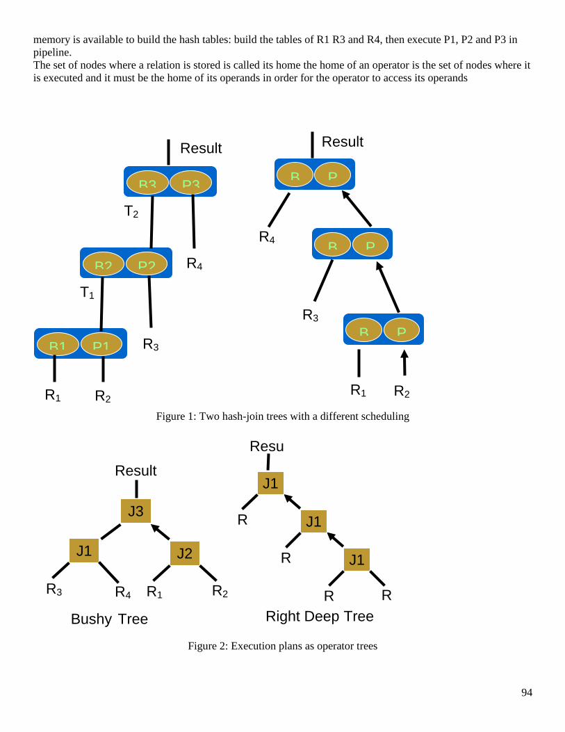
94

memory is available to build the hash tables: build the tables of R1 R3 and R4, then execute P1, P2 and P3 in

pipeline.

The set of nodes where a relation is stored is called its home the home of an operator is the set of nodes where it

is executed and it must be the home of its operands in order for the operator to access its operands

Figure 1: Two hash-join trees with a different scheduling

Figure 2: Execution plans as operator trees

B1 P1

R1 R2

B2 P2

T1

R3

B3 P3

T2

R4

Result

J1

R R

J1

R

J1

R

Result

Right Deep Tree

J2

R1 R2

J1

R3

J3

R4

Result

Bushy Tree

B P

R1 R2

B P

R3

B P

R4

Result

95

Figure 2, shows operator trees that represent execution plans for a three-way join. An operator is a labeled

binary tree where the leaf nodes are relations of the input query and each non-leaf node is an operator node (e.g.

Join, union) whose result is an intermediate relation. A join node captures the join, between its operands

execution annotations are not shown for simplicity. Directed arcs denote that the intermediate relation generated

by a tree node is consumed in pipeline. Operator tree may be linear i.e. at least one operand of each join node is

a base relation or bushy.

It is convenient to represent pipelined relations on as right-hand side input of an operator. Thus, right-deep trees

express full pipelining while left-deep trees express full materialization of intermediate results.

Parallel tree formats other than left or right-deep are also interesting. For example, bushy trees in figure 2 are

the only ones to allow independent parallelism. Independent parallelism is useful when the relations are

partitioned on disjoint homes. Suppose that relations in figure 2 are partitioned two (R1 and R2) by two (R3 and

R4) on disjoint homes (resp. h1 and h2). Then joins j10 and j11 could be independently executed in parallel by

the set of nodes that constitutes h1 and h2

Cost Model

The optimizer cost model is responsible for estimating the cost of a given execution plan. It may consists of two

parts

• Architecture independent

• Architecture dependent

The architecture independent part is constituted by the cost functions for operator algorithms e.g. nested loop

for join and sequential access for select. If we ignore concurrency issues, only the cost functions for data

repartitioning and memory consumption differ and constitute the architecture-dependent part. Indeed,

repartitioning a relation’s tuples in a shared nothing system implies transfers of data across the incorrect,

whereas it reduces o hashing in shared memory systems. Memory consumption in the shared nothing case is

complicated by inter-operator parallelism.

Cost model includes three components:

• Total Work (TW)

• Response Time (RT)

• Memory Consumption (MC)

TW and RT are expressed in seconds and MC in Kbytes. The first two components are used to express a trade-

off between response time and throughput. The third component represents the size of memory needed to

execute the plan. The cost function is a combination of the first two components and plans that need more

memory than available are discarded.

Another approach consist of parameter, specified by the system administrator, by which the maximum

throughput is degraded in order to decrease response time. Given a plan p, its cost is computed by a

parameterized function defined as:

Where WRT and WTW are weight factors between 0 and 1 such that WRT + WTW =1

The total work can be computed by a formula that simply adds all

• CPU time

• I/O time

• Communication time

The response time of p, scheduled in phases (each denoted by ph) is computed as follows:

RT(p) = (maxOp€ph(respTime(Op)+p_delay(Op)) +st_delay(ph))

)()( ,

pWWCost

TWRT

WRT*RT + WTW*TW If MC < available memory, otherwise

96

To estimate the cost of an execution plan, the cost model uses database statistics and organization information,

such as relation cardinalities and partitioning as with distributed query optimization.

Search strategy

The search strategy does not need to be different from either centralized or distributed query optimization. Thus,

randomized search strategies generally outperform deterministic strategies in parallel query optimization.

Summary

Parallel query optimization exhibits similarities should take advantage of both intra-operator parallelism and

inter-operator parallelism. Parallel query optimization refers to the process of producing an execution plan for a

query that minimizes an objective cost function. A query optimizer consists of three components Search Space,

Cost Model and Search Strategy.


Course Code: CS712


Lecture No: 42


- Analysis of Parallel Data Processing Approaches

97



- Object-Oriented concepts

- Object Distribution Design

- Architectural Issues

Introduction:

Database technology is rapidly evolving toward the support of new applications. Relational databases have

proven to be very successful in supporting business data processing applications. There is now an important

class of applications, commonly referred to as “advanced database applications:, that exhibit pressing needs for

database management. Examples include computer-aided design (CAD), office information system (OIS),

multimedia information system and artificial intelligence (AI). For these applications, object database

management systems (object DBMSs) are considered.

Fundamental object concepts and object models

An object DBMS is a system that uses an object as the fundamental modeling and access primitive. Contrary to

relational model, there is no universally accepted and formally specified object model. There are a number of

features that are common to most model specifications, but the exact semantics of these features are different in

each model. Some standard object model specifications are emerging as part of language standards (e.g. Object

Data Management Group’s (ODMG) model or SQL-3 but these are not widely adopted.

Basic Object Concepts

An object represents a real entity in the system that is being modeled. It is represented as a pair (OID, state), in

which OID is the object identity and the corresponding state is some representation of the current state of the

object. In some models, OID equality is the only comparison primitive for other types of comparisons, the type

definer is expected to specify the semantics of comparison. In other models, two objects are said to be identical

if they have the same OID, and equal if they have the same state.

Many object models start to diverge at the definition of state. Some object models define state as either an

atomic value or a constructed value (e.g. tuple or set). Let D be the union of the system-defined domains and of

user-defined abstract data type (ADT) domains, let I be the domain of identifiers used to name objects and let A

be the domain of attribute names. A value is defined as follows:

1. An element of D is a value called an atomic value.

2. [a1: v1,…., an: vn], in which ai is an element of A and vi is either a value or an element of I, is called a

tuple value, [] is known as the tuple constructor.

3. {v1,…., vn}, in which vi is wither a value or an element of I, is called a set value, {} is known as set

constructor.

Object examples

• [i1, 432]

• [i2, ‘DDBS’]

• [i3, {3,9,13}]

• [i4, {i4, i6}]

• [i9, [at1: i5, at2:i6, at3:i7]]

Abstract Data Types

An abstract data type is a template for all objects of that type. An ADT describes the type of data by providing a

domain of data with the same structure, as well as operations (also called methods) applicable o elements of that

domain. The abstraction capability of ADTs, commonly referred to as encapsulation, hides the implementation

details of the operations, which can be written in a general purpose programming language. Each ADT is

identifiable to the outer world by the properties that it supports.

Example of ADT

98

The type definition of Car can be as follows:

type Car {

attributes

engine : Engine

bumpers : {Bumper}

tires: [LF : Tire, RF : Tire, LR : Tire, RR : Tire]

make: Manufacturer

model: String

year : Date

serial_no : String

capacity: Integer

methods

age : Real}

The type definition specifies that Car has eight attributes and one method. Four of the attributes (model, year,

serial_no, capacity) are value-based, while the others (engine, bumpers, tires and make) are object-based.

Advantage of ADT

1. The primitive types provided by the system can easily be extended with user-defined types.

2. ADT operations capture parts of the application programs which are more closely associated with data.

Composition (Aggregation)

Composition is one of the most powerful features of object models it allows sharing of objects, commonly

referred to as referential sharing, since objects refer to each other by their OIDs as values of object-based

attributes.

Example of Composition

Assume that c1 is one instance of Car type which is defined above. If the following is true:

(i2, [name: Tahir, mycar: c1])

(i3, [name: Umer, mycar: c1])

Then this indicates that Tahir and Umer own the same car.

A restriction on composite objects results in complex objects. The difference between a composite and a

complex object is that the former allows referential sharing while the later does not. For example, Car type may

have an attribute whose domain is type Tire. It is not natural for two instances of type Car, c1 and c2, to refer to

the same set of instances of Tire, since one would not expect in real life for tires to be used on multiple vehicles

at the same time.

Class vs type A class represents both a template for all common objects (i.e. servers as a type) and the grouping of these

common objects (i.e. the extent). The database schema consists of s set of class definitions with the

relationships among them.

Conceptually, there is difference between a type and a class. A type is a template for all objects of that type

whereas a class is a grouping of all object instances of a given type. A type corresponds to a relation schema in

relational database, whereas a class corresponds to a populated relation instance.

Collection A collection is a user defined grouping of objects. Most conventional systems provide either the class construct

or the collection construct. Collections provide for a clear closure semantics of the query models and facilitate

definition of user views.

In systems, where both classes and collections are supported, a collection is similar to a class in that it groups

objects, but it differs in the following respects.

99

• Object creation may not occur through a collection, object creation occurs only through classes

• An object may exist in any number of collections, but is a member of only one class

• The management of classes is implicit, in that the system automatically maintains classes based on the

type lattice, whereas the management of collections is explicit, meaning that the user is responsible for

their extents.

Subtyping/Inheritance Object systems provide extensibility by allowing user-defined types to be defined and managed by the system.

This is accomplished in two ways: by the definition of types using type constructors or by the definition of

types based on existing primitive types through the process of subtyping. Subtyping is based on the

specialization relationship among types. A type A’ is a specialization of another type B if its interface is a

subset of B’s interface. Thus, a specialized type is more defined than the type from which it is specialized. A

type may be a specialization of number of types; it is explicitly specified as a subtype of a subset of them.

Subtyping and specialization indicate an is-a relationship between types.

Declaring a type to be a subtype of another results in inheritance. Inheritance allows reuse. A subtype may

inherit either the behavior of its subtype, or its implementation or both. There are two type of inheritance:

• Single Inheritance

• Multiple Inheritance

Object Distribution Design

Distribution design involves fragmentation and allocation. Distribution design in the object world brings new

complexities. Conceptually, objects encapsulate methods together with state. In reality, methods are

implemented on types and shared by all instance objects of that type. The location of objects with respect to

their types becomes an issue.

Distribution design in the object world brings new complexities due to the encapsulation of methods together

with object state. This causes problems because methods are implemented on types and shared by all instance

objects of that type. One has to decide whether fragmentation is performed only on attributes duplicating the

methods with each fragment, or whether one can fragment methods as well.

Horizontal Class Partitioning

There are analogies between horizontal fragmentation of object databases and their relational counterparts. It is

possible to identify primary horizontal fragmentation in the object database case identically to the relational

case. Derived fragmentation shows some differences. In object databases, derived horizontal fragmentation can

occur in a number of ways:

1. Partitioning of a class arising from the fragmentation of its subclasses.

2. The fragmentation of a complex attribute may affect the fragmentation of its containing class.

3. Fragmentation of a class based on a method invocation sequence from one class to another may need to

be reflected in the design.

Vertical Class Partitioning

Vertical fragmentation is considerably more complicated. Given a class C, fragmenting it vertically into C1, C2,

…, Cm produces a number of classes, each of which contains some of the attributes and some of the methods.

Each of the fragments is less defined than the original class.

Path Partitioning

The composition graph presents a representation for composite objects. For many applications, it is necessary to

access the composite object. Path partitioning is a concept describing the clustering of all the objects forming a

composite object into a partition. A path partition consists of grouping the objects of all the domain classes that

correspond to all the instance variables in the subtree rooted at the composite object.

Class Partitioning Algorithms

The algorithms for class partitioning are based on:

• Affinity-based Approach

• Cost-driven Approach

100

Allocation

The data allocation problem for object databases involves allocation of both methods and classes. The methog

allocation problem is tightly coupled to the class allocation problem because of encapsulation. Allocation of

classes will imply allocation of methods to their corresponding home classes. But since applications on object-

oriented databases invoke methods, the allocation of methods affects the performance of applications. Four

alternatives can be identified.

1. Local behavior- local object. This is the most straightforward case and is included to form the baseline

case. The behavior, the object to which it is to be applied, and the arguments are all co-located.

2. Local behavior – remote object. This is one of the cases in which the behavior and the object to which

it is applied are located at different sites.

3. Remote behavior – local object. This case is reverse of case (2).

4. Remote function – remote argument. This is the reverse of case (1).

Architectural Issues

One way to develop a distributed system is the client/server approach. Most of the current object DBMS are

client/server systems. The design issues related to these systems are somewhat more complicated due to the

characteristics of object models. Some of concerns are listed below:

• Unit of communication

• Function provided by Client/Server

• Function shipping vs data shipping

• Pre-fetching option

Summary

We have studied the object-oriented concepts (object, ADT, composition, class vs type, collection and

subtyping/inheritance), object distribution design (Horizontal Class Partitioning, Vertical Class Partitioning,

Path Partitioning, Class Partitioning Algorithms, Allocation) and architectural issues.


Course Code: CS712


Lecture No: 43

101


- Basic OO Concepts

- Started the OODDBS architectures


- Two Alternatives

o Object Server Architecture

o Page Server Architecture

Alternative Client/Server Architectures

Two main types of client/server architectures have been proposed:

1. Object servers

2. Page servers

The distinction is partly based on the granularity of data that is shipped between the client and server and partly

on the functionality provided to the clients and servers.

1) Object Server

Client request objects from the server, which retrieves them from the database and returns them to the

requesting client. These systems are called object servers as shown in figure 1. In object servers, the server

undertakes most of the DBMS services, with the client providing basically an execution environment for the

application as well as some level of object management functionality. The object management layer is

duplicated at both the client and the server in order to allow both to perform object functions. Object manager

serves a number of functions.

102

Figure 1: Object server architecture

Feature of the Object Server Architecture

• Objects move between clients and servers

• Object Manager helps to execute methods on both sides

Server Side Functions

Server side performs following functions

• OID implementation; it is tricky to manage OID in RAM and Disk

• Object Caching

• Object shipment between clients and servers can be optimized depending on type of clustering

• Lock management needed when same object being accessed (read, modified) at different places

• Persistent placement of objects

Page Server

The unit of transfer between the servers and the clients is a physical unit of data, such as a page or segment,

rather than an object as shown in figure 2.

Applicatio

Query Interface

Object Browser

Programmatic Interface

Objects

Network

Client

Object Manager

Query Optimizer

Lock Manager

Storage

Page Cache Manager

Server

Object Database

103

Figure 2: page server architecture

Feature of Page Server Architecture

• Data moves in the form of pages rather than objects

• Object management mainly performed at the client side

• Data management at the server side

Comparison

• One can’t be declared better absolutely

• If object access pattern resembles storage pattern, then page server is better

• Object server provides better concurrency as object based locking lets multiple client access objects

from the same page

• Object server ships only the required objects, so data transferred is reduced

Other Issues

1) Client Buffer Management

Client can manage either a

• Page buffer

• Object buffer

• Page/Object buffer

If client has a page buffer then entire pages are read or written from the server every time a page fault occurs or

a page is flushed. Object buffers can read/write individual objects and allow the applications object-by-object

access.

Applicatio

Query Interface Object

Browser Programmatic

Interface

Pages

Network

Client

Object Manager

Query Optimizer

Lock Manager

Storage

Page Cache Manager

Server

File and Index Manager

Page and Cache Manager

Object Database

104

Object buffers manage access at a finer granularity and can achieve higher levels of concurrency. However,

they may experience buffer fragmentation as the buffer may not able to accommodate an integral multiple of

objects, thereby leaving some unused space. A page buffer does not encounter this problem, but if the data

clustering on the disk does not match the application data access pattern, then the pages contain a great deal of

unaccessed objects that use up valuable client buffer space.

In a page/object buffer, the client loads pages into the page buffer. When the client flushes out a page, it retains

the useful objects from the page by copying the objects into the object buffer. The client buffer manager tries to

retain well-clustered pages and isolated objects from non-well clustered pages. The client buffer managers

retain the pages and objects across the transaction boundaries.

2) Server Buffer Management

The server buffer management issues do not change in object client/server systems, since the servers usually

manage a page buffer. The pages from the page buffer are sent to the clients to satisfy their data requests. A

grouped object-server constructs its object groups by copying the necessary objects from the relevant server

buffer pages, and sends the object group to the clients. Servers can also maintain the modified object buffer

(MOB). A MOB stores objects that have been updated and returned by the clients.

Cache Consistency

Cache maintained at the server side. Data access from multiple clients becomes efficient but requires

consistency maintained. The DMS cache consistency algorithms can be classified as

1) Avoidance bases: stale data (cached and updated) should not be given access

2) Detection based: stale data given to different clients, consistency checked before finally moving to disk

Both algorithms further can be classified as

1) Synchronous: the client sends a lock escalation message at the time it wants to perform a write

operation and it blocks until the server responds.

2) Asynchronous: the client sends a lock escalation message at the time of its write operation but does not

block waiting for a server response.

3) Deferred: the client optimistically defers informing the server about its write operation until commit

time.

Object Management

Three issues of object management are discussed here

1) OID Management

2) Pointer Swizzling

3) Object Migration

1) Object Identifier Management

OID:

• OID’s are system generated and used to uniquely identify every object in the system

• OID management applies to any OO-environment

• OID is important for both transient and persistent objects

• For persistent objects, OIDs can be physical or logical

• Physical OID helps management of objects on disk

• It is problematic when objects’ location is required to be changed frequently

Logical OID:

• Logical OID/Surrogate: independent of physical position of object

• Could be initiated using many different schemes

• May require to maintain a lookup table

An Example Lookup Table

105

OID Disk Location

1 A678BE8

2 A678B12

3 45368BA

4 C765984

5 657904

6 564098

7 34689AB

• Lookup table can be cached for efficiency

• However introduces an extra reference, that is, in lookup table

• Logical ID is efficient in case object movement is frequent, since it requires change in lookup table only

• OID management becomes more complicated in DDBS environment

• Requires uniqueness across multiple servers

• One possibility is to assign responsibility of generating OIDs to one server

• Any object created anywhere requests this server for OID

• Uniqueness is easy to maintain, but may become bottleneck

• Secondly, every server generates OIDs for its own objects

• Requires server ID to become the part of OID to ensure system-wide uniqueness

2) Pointer Swizzling

Objects when brought into RAM from disk, their OIDs have to be transformed to RAM address; this process is

called pointer swizzling. Pointer swizzling can be lookup table based. Hardware based use the page fault

mechanism for pointer swizzling.

3) Object Migration

One aspect of distributed systems is that objects move, from time to time, between sites. This raises a number

of issues. First is the unit of migration. In systems where the state is separated from the methods, it is possible to

consider moving the object’s state without moving the methods. Another issue is that the movements of the

objects must be tracked so that they can be found in their new locations. The migration of objects can be

accomplished based on their current state.

Object states:

Objects can be in one of four states:

1) Ready

2) Active

3) Waiting

4) Suspended

Objects in active or waiting state are not allowed to migrate, since the activity they are currently involved in

would be broken. The migration involves two steps:

1) Shipping the object from the source to the destination

2) Creating a proxy at the source, replacing the original object

Distributed Object Storage Two issues related to the object storage are:

1) Object clustering

2) Distributed garbage collection

1) Object Clustering

Object clustering refers to the grouping of objects in physical containers (i.e. disk extents) according to common

properties, such as the same value of an attribute or sub-objects of same object. Thus fast access to clustered

objects can be obtained.

106

Object clustering is difficult for two reasons.

1) It is not orthogonal to object identity implementation

2) The clustering of complex objects along the composition relationship is more involved because of object

sharing

Models of object clustering

There are three basic models for object clustering

Decomposition of storage model (DSM)

Normalized storage model (NSM)

Direct storage model

2) Distributed Garbage Collection

This is the common issue in OS and Databases Objects that are not accessed by any access routine become

garbage. We have to identify such objects and re-claim memory occupied them by destroying objects. The basic

garbage collection algorithms can be categorized as

Reference counting

Tracing based

Reference counting

Each object has an associated count of the references to it.

Tracing based

Tracing based collectors are divided into

• Mark and sweep: periodically follows the hierarchy of the objects to detect that are not being accessed

• Copy based: copy the objects that are accessed and delete the remaining

Summary

• Architectures of OODDBS

• Different Issues

– Storage Management

– OID Handling

– Cache Management

– Pointer Swizzling

– Object Migration

– Garbage Collection


Course Code: CS712


Lecture No: 44

107


- Two Alternatives

o Object Server Architecture

o Page Server Architecture


- Transaction management in distributed OODBMS

- Database interoperability

Transaction Management

Here we are discussing some issues that arise in extending the transaction concept to object DBMSs. Most

object DBMSs maintain page level locks or concurrency control and support the traditional flat transaction

model. It has been argued that the traditional flat model would not meet the requirements of the advanced

application domains that object data management technology would serve. Some of the considerations are that

transactions in these domains are longer in duration, requiring interactions with the user or the application

program during their execution. In the case of object systems, transactions do not consist of simple read/write

operations. In some application domains the fundamental transaction synchronization paradigm based on

competition among transactions for access to resources must change to one of cooperation among transactions

in accomplishing a common task.

Requirement for transaction management

The requirements for transaction management in object DBMSs are:

1) Conventional transaction managers synchronize simple read and write operations. Their counterparts for

object DBMSs must be able to deal with abstract operations.

2) Conventional transactions access flat objects (e.g. pages, tuples) whereas transactions in object DBMS

require synchronization of access to composite and complex objects.

3) Some applications supported by object DBMSs have different database access patterns than

conventional database applications, where the access is competitive.

Correctness Criteria

Three alternatives

• Commutativity

108

• Invalidation

• Recoverability

1) Commutativity

It states that two operations conflict if the results serial execution of these operations are not equivalent.

Consider the simple operations R(x) and W(x). if nothing is known about the abstract semantics of the Read and

Write operations or the object x upon which they operate, it has to be accepted that a R(x) following a W(x)

does not retrieve the same value as it would prior to the W(x). a write operation always conflicts with other

Read or Write operations.

Commutativity Types

There are two types

• Forward Commutativity

• Backward Commutativity

Forward Commutativity: two operations P and Q and a state s of object, then

“For every state s in which P and Q are both defined, P(Q(s)) = Q(P(s)) and P(Q(s)) is defined(i.e. it is not the

null state)”

Backward Commutativity: “ For every state s in which we know P(Q(S)) is defined P(Q(s)) = Q(P(a))”

Example:

The forward and backward compatibility relations for the set ADT are given in figure 1 and figure 2

respectively.

An operation is defined as a pair of invocation and response to that invocation e.g. x:[Insert(3),ok] is a valid

invocation of an insert operation on set x that returns that the operation was performed correctly.

Compatibility Table for Forward Commutativity

[Insert(i), ok] [Delete(i), ok] [Member(i), tr] [Member(i), fl]

[Insert(i), ok] + - + -

[Delete(i), ok] - + + +

[Member(i), tr] + - + +

[Member(i), fl] - + + +

Figure 1: Compatibility Table for Forward Commutativity in Sets

Compatibility Table for Backward Commutativity

[Insert(i), ok] [Delete(i), ok] [Member(i), tr] [Member(i), fl]

[Insert(i), ok] + - - -

109

[Delete(i), ok] - + - +

[Member(i), tr] - - + +

[Member(i), fl] - + + +

Figure 2: Compatibility Table for Backward Commutativity

2) Invalidation

An operation P invalidates Q, if there are two histories H1, H2 such that H1 * P * H2 and H1 * H2 * Q are

defined but H1 * P * H2 * Q isn’t.

3) Recoverability

An operation P is said to be recoverable with respect to operation Q if the value returned by P is independent of

whether Q executed before P or not.

Database Interoperability

Database integration: involves the process by which information from participating databases can be

conceptually integrated to form a single cohesive definition of a multidatabase.

Generally meant in an multi-database (MDBS) environment; a complex database environment

• Databases are heterogeneous

• Architecture could be global schema architecture as shown in figure 3 or the federated database

architecture

• Participating databases are autonomous

Heterogeneity could be

• Hardware

• Software

• Data Models

• Semantic

In all other DBS architectures, databases are owned by a single organization. So no semantic heterogeneity

Global Schema Architecture

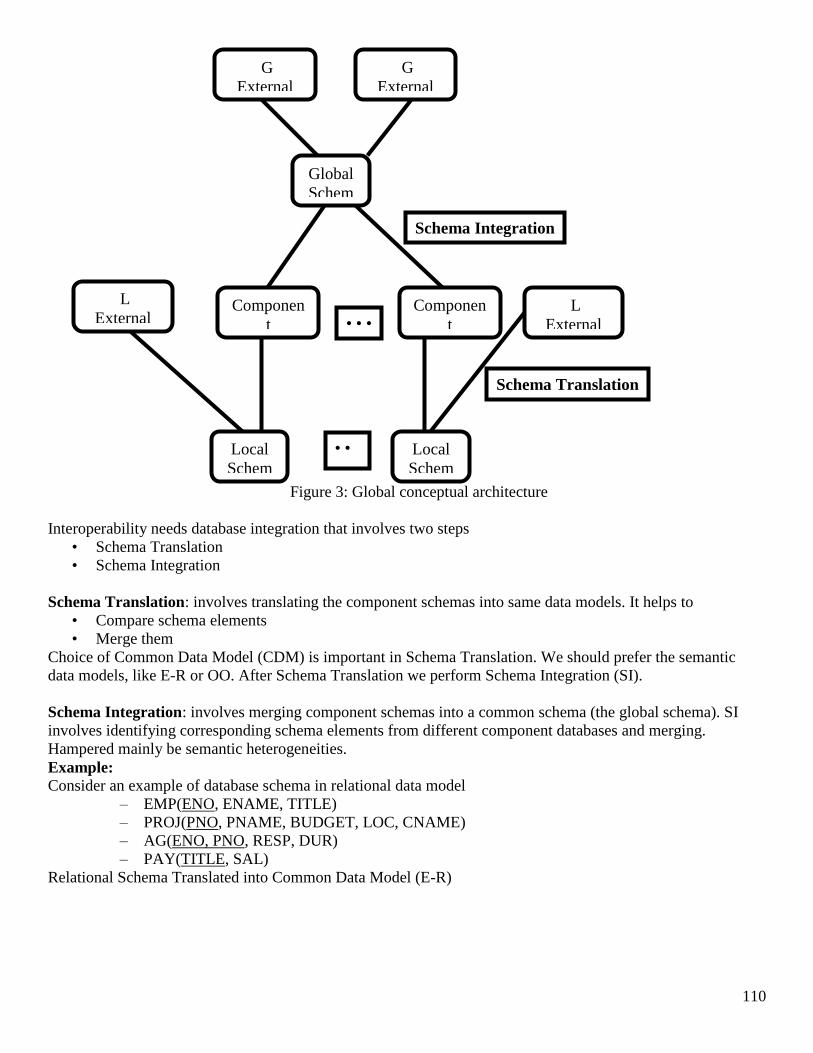
110

Figure 3: Global conceptual architecture

Interoperability needs database integration that involves two steps

• Schema Translation

• Schema Integration

Schema Translation: involves translating the component schemas into same data models. It helps to

• Compare schema elements

• Merge them

Choice of Common Data Model (CDM) is important in Schema Translation. We should prefer the semantic

data models, like E-R or OO. After Schema Translation we perform Schema Integration (SI).

Schema Integration: involves merging component schemas into a common schema (the global schema). SI

involves identifying corresponding schema elements from different component databases and merging.

Hampered mainly be semantic heterogeneities.

Example:

Consider an example of database schema in relational data model

– EMP(ENO, ENAME, TITLE)

– PROJ(PNO, PNAME, BUDGET, LOC, CNAME)

– AG(ENO, PNO, RESP, DUR)

– PAY(TITLE, SAL)

Relational Schema Translated into Common Data Model (E-R)

L

External

G

External

Schema

Global

Schem

Componen

t

Schema

Componen

t

Schema

• • •

Local

Schem

Local

Schem

• •

•

Schema Translation

Schema Integration

G

External

L

External

Schema

111

Figure 4: Entity-Relationship Database

Approaches to SI

• Binary: Two schemas merged first, then one at a time

• N-ary: All compared and merged together

Steps in SI

• Schema Analysis/Matching

• Schema Conforming

• Schema Merging

Heterogeneities

Two types of heterogeneity:

1) Semantic Heterogeneity: same concepts modeled differently in different schemas:

Example: naming, aggregation, generalization, attribute class, default value, database identifier, schema

isomorphism, missing values

2) Structural Heterogeneity: differences in the representation of corresponding schema elements

Examples: Data scaling and precision, attribute integrity constraint, objects included, domain

Heterogeneities are resolved by applying the mapping on elements. We cannot ask/expect the component

databases to change. Most common semantic is naming conflict that could be Synonyms and Homonyms.

Synonyms: different names modeling same thing, like in our example schema ENGINEER/ EMP and

Salary/Sal.

Homonym: same name modeling different things, like title here.

Summary

EMP

ENO ENAME

PROJ

PNO PNAME

BUDGET LOC DUR

CNAME

ASG

RESP

PAY

TITLE

SAL

PAYMENT

1

N

N M

112

We have discussed the transaction management (TM), requirements of TM and Correctness Criteria.

Correctness criteria consist of Commutativity, Invalidation, and Recoverability. Database Interoperability also

discussed.


Course Code: CS712


Lecture No: 45


- Transaction management in distributed OODBMS

- Database interoperability


- Database interoperability (continued..)

113

Database Interoperability (continued..)

Architecture is global schema multidatabase system. Objective is to merge the schemas of the component

databases and present as a single schema. Data is owned by different organization. User does not have any idea

about it. Interoperability involves

• Schema translation

• Schema integration

Steps in SI

• Schema Analysis/Matching

• Schema Conforming

• Schema Merging

Schema integration is an older issue than the DDBSs. In initial days of database design it was being performed

view integration View integration is simpler as compare to SI. Context is same, as database is being developed

for the same organization

SI is more complex,

• autonomous schemas contain heterogeneities even if they belong to same domain

• Schemas contain data that also needs to be merged

Early SI approaches were mainly influenced by view integration.

Schema Analysis/Matching

Initially correspondence finding phase was called schema analysis; today it is called schema matching.

Schema Conforming: resolving differences among the elements modeling same/similar elements

Schema merging: combining those elements.

Most challenging task in SI is establishing correspondences among schema elements. Reason: the existence of

semantic heterogeneities

Heterogeneities

Two types of heterogeneity:

Semantic heterogeneity: same concepts modeled differently in different schemas:

Example: naming, aggregation, generalization, attribute class, default value, database identifier, schema

isomorphism, missing values

Structural heterogeneity: differences in the representation of corresponding schema elements

Example: Data scaling and precision, attribute integrity constraint, objects included, domain

Semantic heterogeneity:

Most common semantic is naming conflict that could be Synonyms and Homonyms

Synonyms: different names modeling same thing, like in our example schema ENGINEER/ EMP and

Salary/Sal as shown in figure 1.

Homonym: same name modeling different things, like title here.

SI cannot be performed totally automatically. We need to know the semantics for establishing correspondences.

Source for semantics is schema. Current data models do not capture the real-world semantics completely. So

meaning is either in the mind of designer or it is in the application programs. So we cannot completely automate

SI. Doing it manually is also not possible, as it is a huge process. So we should perform SI semi-automatically.

There are different approaches to do the SI A very common approach is ontology based

Ontologies

An ontology is an application dependent collection of terms, their meaning and possibly relation between them.

Naming conflicts are removed by adopting names from ontology in the global schema and mapping component

114

elements to them. One approach could be to map the schema elements to the concepts/terms in the ontology.

We do this once for all schemas. After mapping all the schemas we compare the ontological terms rather than

the elements. Comparison becomes sort of free of at least naming conflicts.

Most important is SA/SM. Takes two or more schemas as input and generates matching assertions. Different

forms of assertions are there. Schema matching approaches is now described by the matcher they use. Initial

classification was mainly the syntactic and semantic based. Today, matchers are established. Famous matchers

are:

• Name based

• Description based

• Global namespaces

• Type based

• Key similarity

• Instance based

• Some even use Neural Networks

Then there is concept of combining matchers. We have hybrid and composite approaches of combining

matchers Some Schema Matching approaches

• Autoplex, SKAT, Dike, COMA, TransScm etc.

Most of the matchers assign strength to assertions. Value ranges between 0 and 1. Matchers suggest the strong

candidate assertions and user/ integrator finalizes them

Structural Heterogeneities

Entity versus attribute, like client. Attribute has to be transformed into entity in the global schema and mapping

to be established. Dependency, relationship is one to many or many to many, have to adopt more general one

Synonym

Figure 1: synonyms

Entity vs attribute

Figure 2

For example, cardinality difference

115

Figure 3

Schema conforming aligns them from merging, mainly structural conflicts, example.

Figure 4

Overview of the course

• Introduction to distributed systems and their justification

• Basics of Databases, specially relational data model and networks

• Architectures in DDBSs

• Design issues, fragmentation, its types, PHF, DHF, VF, Hybrid

• Experiments/Particles of DDBS implementation

• Transaction Management basics and then in DDBS environment

• Then query processing

• Parallel databases

• Object Oriented Databases

• Database Interoperability

Thank you very much, hope you have enjoyed the course

Course Title: Distributed Database Management Systems ... to 45 lectures.pdf · C50001 Suhail...

Documents

Transcript of Course Title: Distributed Database Management Systems ... to 45 lectures.pdf · C50001 Suhail...