PHYSICAL REVIEW E 83, 011915 (2011)

Calculations of the second virial coefficients of protein solutions withan extended fast multipole method

Bongkeun Kim and Xueyu SongDepartment of Chemistry, Iowa State University, Ames, Iowa 50011, USA

(Received 21 October 2010; published 27 January 2011)

The osmotic second virial coefficients B2 are directly related to the solubility of protein molecules in electrolytesolutions and can be useful to narrow down the search parameter space of protein crystallization conditions. Usinga residue level model of protein-protein interaction in electrolyte solutions B2 of bovine pancreatic trypsin inhibitorand lysozyme in various solution conditions such as salt concentration, pH and temperature are calculated usingan extended fast multipole method in combination with the boundary element formulation. Overall, the calculatedB2 are well correlated with the experimental observations for various solution conditions. In combination withour previous work on the binding affinity calculations it is reasonable to expect that our residue level model canbe used as a reliable model to describe protein-protein interaction in solutions.

DOI: 10.1103/PhysRevE.83.011915 PACS number(s): 87.10.−e

I. INTRODUCTION

In a remarkable observation, George and Wilson foundthat there is a correlation between slightly negative secondvirial coefficient of a protein solution and its successfulcrystallization condition [1]. There is also a correlationbetween the solubility of a protein in an electrolyte solutionand the osmotic second virial coefficient B2 of the solution(Veesler et al. [2], Boistelle et al. [3]). These observationshave led to numerous studies on the second virial coefficientsof protein solutions with the hope to use this property tonarrow down the parameter space of protein solutions for thesearch of optimal crystallization conditions. For example, evenfor membrane proteins, rapid screening of small moleculesand detergents as crystallization additives are achieved toimprove the crystallization conditions of light harvestingprotein complexes [4].

Experimentally, the osmotic second virial coefficients B2

can be measured by using Static Light Scattering (SLC)[1,5,6], Small Angle X-ray Scattering (SAXS) [7], SmallAngle Neutron Scattering (SANS) [8], or Self-InteractionChromatography (SIC) [9]. All of these methods, however,are quite demanding due to large amounts of proteins used inthe measurements. So far, using the B2 of protein solutions asa tool to screen the solution conditions is not a routine practiceyet in most crystallographers’ labs.

To overcome the protein consumption problem in B2

measurements, one possible alternative is to use computationalmethods to calculate the second virial coefficients of proteinsolutions. B2 is related to molecular interactions in terms ofthe orientationally averaged potential of mean force (PMF),W (r12), where r12 is the center-to-center distance,

B2 = −2π

∫ ∞

0(e−W (r12)/kBT − 1)r2

12dr12, (1)

where W is the interaction free energy between two proteins,kB is the Boltzmann constant, and T the temperature. Previousefforts to model the interaction free energy between twoprotein molecules and to compute B2 have been based onidealized descriptions of proteins. The protein molecules aremostly treated as spheres, although Vilker et al. [10] modeleda protein (bovine serum albumin) as an ellipsoid. For spherical

model approaches, the interaction is normally divided into twoparts: The first part is due to the excluded volume to account forthe size of protein molecules and the second part accounts forthe solution dependent effective interaction between proteinmolecules. Due to the spherical shape approximation ofprotein molecules, the thickness of the hydration layer is oftenconsidered as an adjustable parameter for B2 calculations.The solution dependent contributions to B2 are modeled usingstandard colloidal methods [11]. Namely the van der Waalsinteraction is treated in the Lifshitz-Hamaker framework andthe electrostatic interaction [10,12–14] is obtained using thePoisson-Boltzmann approach. For such idealized sphericalmodels, with adjustable parameters such as the Hamakerconstant the computed B2 have been partially successful tocapture the trend of experimental data at various solutionconditions.

Neal et al. [15] calculated the second virial coefficients byapplying orientational dependence protein-protein interactionmodels. Electrostatic interactions in their study were obtainedby distributing charges to the ionizable residues, thus an orien-tationally dependent charge distribution but treating the proteinas a spherical dielectric body. The van der Waals interactionswere calculated by a semiempirical approach. When theintermolecular distance is large enough, the Lifshitz-Hamakerapproach [16] was implemented with the realistic shapeof proteins in mind. At shorter distance, the OptimizedPotentials for Liquid Simulations (OPLS) parameter set[17] was used to capture the short-range interaction. Eventhough the comparison between their calculations andexperimental measurements yields large errors for some B2

calculations, this approach did not use any further adjustableparameters.

The goal of our work is to develop a protein-proteininteraction model to account for the realistic shape ofproteins and at the same time to capture the effect ofsolutions without adjustable parameters. To this end, aresidue level model of protein-protein interaction had beenintroduced [18,19].

In this model, each residue of a protein is representedby a sphere located at the geometric center of the residuedetermined by its native or approximate structure. The

011915-11539-3755/2011/83(1)/011915(15) ©2011 American Physical Society

BONGKEUN KIM AND XUEYU SONG PHYSICAL REVIEW E 83, 011915 (2011)

diameter of the sphere is determined by the molecular volumeof a residue in a solution environment [20]. The molecularsurface of our model protein is defined as the Richard-Connolly surface spanned by the union of these residuespheres using the MSMS program from Sanner [21]. Eachresidue carries a permanent dipole moment located at thecenter of its sphere and the direction of the dipole is givenby the amino acid type from the protein’s native structure.If a residue is charged the amount of charge is given bythe Henderson-Hasselbalch equation using the generic pKa

values of residues if the local environmental effects on pKa

values are neglected. Alternatively experimental or calculatedpKa values of residues can be used to account for thelocal environments as it was done in this paper. For eachresidue there is also a polarizable dipole at the center ofthe sphere, whose nuclear polarizability had been determinedfrom our recent work [22] and the electronic polarizabilityis estimated from optical dielectric constant augmented withquantum chemistry calculations [23]. There are three kindsof interactions in this model: the electrostatic interactiondue to the electric double layer effect, the van der Waalsattraction due to the polarizable dipoles and a short-rangecorrection term to account for the short-range interactionssuch as the desolvation energy, hydrophobic interaction, andso on. In this article, we only consider the electrostaticinteraction which gives the most contribution to the protein-protein interaction [24,25], the van der Waals interaction,and the short-range interaction which is accounted for usingthe excluded volume based upon the realistic shape of aprotein.

The electrostatic problem in the electrostatic and the vander Waals interaction is solved using the Poisson-Boltzmannequation where the realistic shapes of protein moleculesare considered. The Boundary Element Method (BEM) incombination with the Fast Multipole Method [26,27] isimplemented to circumvent the extensive memory problemsimilar to the recent work by Lu et al. [28]. The validity ofour model was already tested by binding affinity calculationsof several protein complexes [29]. Direct comparisons be-tween our calculations of B2 and experimental measurementsunder various solution conditions were made and reasonableagreements from these comparisons provide further concreteevidence that our model can be used as a universal model forstudies of nonspecific protein-protein interactions in aqueoussolutions.

II. THEORETICAL DEVELOPMENT

A. General formulation for the second virial coefficientcalculation using a residue level patch model

The osmotic second virial coefficient (B2) can beexpressed in terms of the interaction energy between twoproteins [30]:

B2 = −V

2

[2Q2(T )

Q21(T )

− 1

], (2)

where Q1 and Q2 are one-protein and two-protein partitionfunctions and V is the volume. Noting that the partitionfunction involves the integration of the center of mass

R = (x,y,z) in a space-fixed Cartesian coordinate and therotational coordinates � = (α,β,γ ) in Euler angles, we have

B2 = − 1

128π4V

∫· · ·

∫[e−W (R1,�1,R2,�2)/kBT − 1]

× dR1d�1dR2d�2, (3)

where the interaction potential W describes the anisotropicinteraction between two proteins. dRi = dxidyidzi and d�i =dαi sin βidβidγi . After a transformation to the center of mass ofthe protein pair and to the relative coordinates R = R1 − R2,we assume that protein 1 is in the space-fixed coordinate,thus, the interaction potential W is now independent of �1.The integration over the center of mass of the protein paircoordinate and �1 for B2 yields

B2 = − 1

16π2

∫ ∞

0

∫ π

0

∫ 2π

0

∫ 2π

0

∫ π

0

∫ 2π

0

× [e−W (R,θ,φ,α2,β2,γ2)/kBT − 1]

×R2dR sin θdθdφdα2 sin β2dβ2dγ2. (4)

In this expression of the orientation dependent potentialW (R,θ,φ,α2,β2,γ2), protein 2 moves around protein 1 and(α2,β2,γ2) capture all of the orientations of protein 2 relativeto the space-fixed coordinate (R,θ,φ) of protein 1 (Fig. 1 ).

In our residue level protein-protein interaction model,there are three contributions to the interaction energyW (R,θ,φ,α2,β2,γ2). The electrostatic interaction and the vander Waals interaction will be obtained in the next two sectionswhen the protein molecules are not in contact with each other.When the protein molecules are in contact a simple excludedvolume model will be used. Thus, Eq. (4) can be split into two

FIG. 1. (Color online) Schematic illustration showing the for-mulation of the electrostatic interaction between two proteins. Theorientation of protein 1 (signified by a triangle on protein 1) isdefined by two spherical coordinate angles (θ,φ) in a space-fixedcoordinate (X,Y,Z). The orientation of protein 2 (signified by atriangle on protein 2) is specified by Euler angles (α,β,γ ) relativeto the space-fixed coordinate. The molecular surfaces are defined by∑

1 and∑

2 for each protein and the n1 and n2 are the outward unitnormals on

∑1 and

∑2. ε1 and ε2 are the dielectric constants of the

protein cavity and the solution, respectively. κ represents the inverseDebye screening length. Charge qi and dipole μi are located at thegeometric center ri of residue i.

011915-2

CALCULATIONS OF THE SECOND VIRIAL . . . PHYSICAL REVIEW E 83, 011915 (2011)

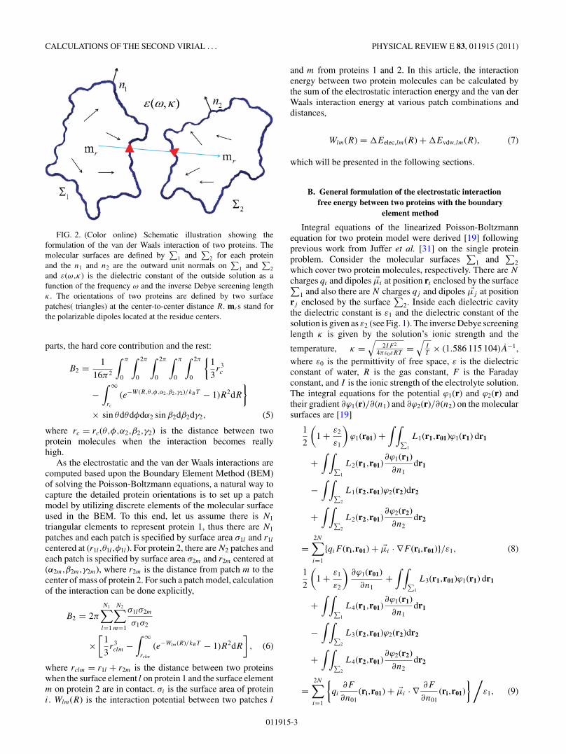
FIG. 2. (Color online) Schematic illustration showing theformulation of the van der Waals interaction of two proteins. Themolecular surfaces are defined by

∑1 and

∑2 for each protein

and the n1 and n2 are the outward unit normals on∑

1 and∑

2

and ε(ω,κ) is the dielectric constant of the outside solution as afunction of the frequency ω and the inverse Debye screening lengthκ . The orientations of two proteins are defined by two surfacepatches( triangles) at the center-to-center distance R. mrs stand forthe polarizable dipoles located at the residue centers.

parts, the hard core contribution and the rest:

B2 = 1

16π2

∫ π

0

∫ 2π

0

∫ 2π

0

∫ π

0

∫ 2π

0

{1

3r3c

−∫ ∞

rc

(e−W (R,θ,φ,α2,β2,γ2)/kBT − 1)R2dR

}× sin θdθdφdα2 sin β2dβ2dγ2, (5)

where rc = rc(θ,φ,α2,β2,γ2) is the distance between twoprotein molecules when the interaction becomes reallyhigh.

As the electrostatic and the van der Waals interactions arecomputed based upon the Boundary Element Method (BEM)of solving the Poisson-Boltzmann equations, a natural way tocapture the detailed protein orientations is to set up a patchmodel by utilizing discrete elements of the molecular surfaceused in the BEM. To this end, let us assume there is N1

triangular elements to represent protein 1, thus there are N1

patches and each patch is specified by surface area σ1l and r1l

centered at (r1l ,θ1l ,φ1l). For protein 2, there are N2 patches andeach patch is specified by surface area σ2m and r2m centered at(α2m,β2m,γ2m), where r2m is the distance from patch m to thecenter of mass of protein 2. For such a patch model, calculationof the interaction can be done explicitly,

B2 = 2π

N1∑l=1

N2∑m=1

σ1lσ2m

σ1σ2

×[

1

3r3clm −

∫ ∞

rclm

(e−Wlm(R)/kBT − 1)R2dR

], (6)

where rclm = r1l + r2m is the distance between two proteinswhen the surface element l on protein 1 and the surface elementm on protein 2 are in contact. σi is the surface area of proteini. Wlm(R) is the interaction potential between two patches l

and m from proteins 1 and 2. In this article, the interactionenergy between two protein molecules can be calculated bythe sum of the electrostatic interaction energy and the van derWaals interaction energy at various patch combinations anddistances,

Wlm(R) = Eelec,lm(R) + Evdw,lm(R), (7)

which will be presented in the following sections.

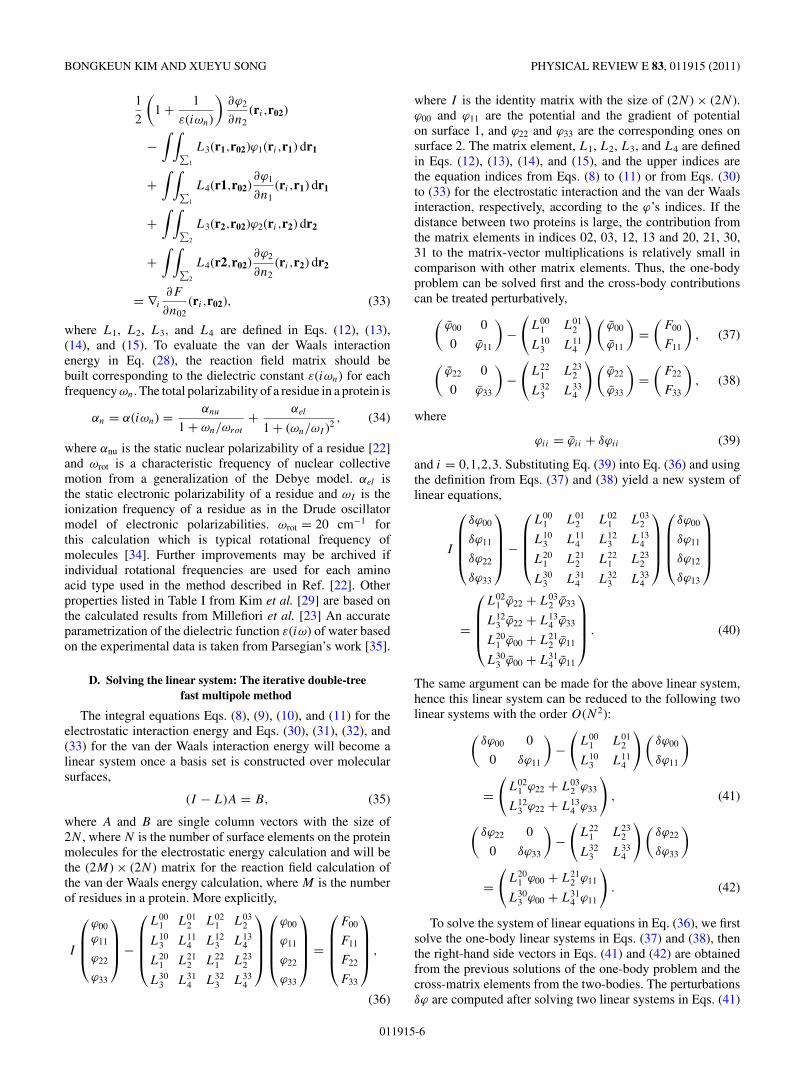
B. General formulation of the electrostatic interactionfree energy between two proteins with the boundary

element method

Integral equations of the linearized Poisson-Boltzmannequation for two protein model were derived [19] followingprevious work from Juffer et al. [31] on the single proteinproblem. Consider the molecular surfaces

∑1 and

∑2

which cover two protein molecules, respectively. There are N

charges qi and dipoles �μi at position ri enclosed by the surface∑1 and also there are N charges qj and dipoles �μj at position

rj enclosed by the surface∑

2. Inside each dielectric cavitythe dielectric constant is ε1 and the dielectric constant of thesolution is given as ε2 (see Fig. 1). The inverse Debye screeninglength κ is given by the solution’s ionic strength and the

temperature, κ =√

2IF 2

4πε0εRT=

√IT

× (1.586 115 104)A−1,where ε0 is the permittivity of free space, ε is the dielectricconstant of water, R is the gas constant, F is the Faradayconstant, and I is the ionic strength of the electrolyte solution.The integral equations for the potential ϕ1(r) and ϕ2(r) andtheir gradient ∂ϕ1(r)/∂(n1) and ∂ϕ2(r)/∂(n2) on the molecularsurfaces are [19]

1

2

(1 + ε2

ε1

)ϕ1(r01) +

∫ ∫∑

1

L1(r1,r01)ϕ1(r1) dr1

+∫ ∫

∑1

L2(r1,r01)∂ϕ1(r1)

∂n1dr1

−∫ ∫

∑2

L1(r2,r01)ϕ2(r2)dr2

+∫ ∫

∑2

L2(r2,r01)∂ϕ2(r2)

∂n2dr2

=2N∑i=1

{qiF (ri,r01) + �μi · ∇F (ri,r01)}/ε1, (8)

1

2

(1 + ε1

ε2

)∂ϕ1(r01)

∂n1+

∫ ∫∑

1

L3(r1,r01)ϕ1(r1) dr1

+∫ ∫

∑1

L4(r1,r01)∂ϕ1(r1)

∂n1dr1

−∫ ∫

∑2

L3(r2,r01)ϕ2(r2)dr2

+∫ ∫

∑2

L4(r2,r01)∂ϕ2(r2)

∂n2dr2

=2N∑i=1

{qi

∂F

∂n01(ri,r01) + �μi · ∇ ∂F

∂n01(ri,r01)

}/ε1, (9)

011915-3

BONGKEUN KIM AND XUEYU SONG PHYSICAL REVIEW E 83, 011915 (2011)

1

2

(1 + ε2

ε1

)ϕ2(r02) −

∫ ∫∑

1

L1(r1,r02)ϕ1(r1) dr1

+∫ ∫

∑1

L2(r1,r02)∂ϕ1(r1)

∂n1dr1

+∫ ∫

∑2

L1(r2,r02)ϕ2(r2)dr2

+∫ ∫

∑2

L2(r2,r02)∂ϕ2(r2)

∂n2dr2

=2N∑i=1

{qiF (ri,r02) + �μi · ∇F (ri,r02)}/ε1, (10)

1

2

(1 + ε1

ε2

)∂ϕ2(r02)

∂n2−

∫ ∫∑

1

L3(r1,r02)ϕ1(r1) dr1

+∫ ∫

∑1

L4(r1,r02)∂ϕ1(r1)

∂n1dr1

+∫ ∫

∑2

L3(r2,r02)ϕ2(r2)dr2

+∫ ∫

∑2

L4(r2,r02)∂ϕ2(r2)

∂n2dr2

=2N∑i=1

{qi

∂F

∂n02(ri,r02) + �μi · ∇ ∂F

∂n02(ri,r02)

}/ε1, (11)

where

L1(r,r0) = ∂F

∂n(r,r0) − ε2

ε1

∂P

∂n(r,r0), (12)

L2(r,r0) = P (r,r0) − F (r,r0), (13)

L3(r,r0) = ∂2F

∂n0∂n(r,r0) − ∂2P

∂n0∂n(r,r0), (14)

L4(r,r0) = − ∂F

∂n0(r,r0) + ∂P

∂n0(r,r0)

ε1

ε2, (15)

and

F (r,r0) = 1

4π |r − r0| ,(16)

P (r,r0) = e−κ|r−r0|

4π |r − r0| .

Although the traditional boundary element method such asAtkinson and his coworkers [32] can be used to solve the aboveintegral equations, the memory requirement is too costly forcurrent computers using either a direct linear system solver oran iterative solver, such as the Generalized Minimal ResidualMethod (GMRES) for a moderate size protein. In the currentwork the Fast Multipole Method is used and the details of ourimplementation will be outlined in Secs. II D and II E. Oncethe above integral equations are solved the potentials insidethe dielectric cavity are

ϕ1(r1) = −∫ ∫

∑1

L1(r1,r01)ϕ1(r01) dr01

−∫ ∫

∑1

L2(r1,r01)∂ϕ1(r01)

∂n01dr01, (17)

ϕ2(r2) = −∫ ∫

∑2

L1(r2,r02)ϕ2(r02) dr02

−∫ ∫

∑2

L2(r2,r02)∂ϕ2(r02)

∂n02dr02, (18)

∇1ϕ1(r1) = −∫ ∫

∑1

∇1L1(r1,r01)ϕ1(r01) dr01

−∫ ∫

∑1

∇1L2(r1,r01)∂ϕ1(r01)

∂n01dr01, (19)

∇2ϕ2(r2) = −∫ ∫

∑2

∇2L1(r2,r02)ϕ2(r02) dr02

−∫ ∫

∑2

∇2L2(r2,r02)∂ϕ2(r02)

∂n02dr02. (20)

The electrostatic free energy between the protein moleculesat a center-to-center distance, R, and relative orientations,�1 = (θ,φ) and �2 = (α2,β2,γ2), is given by

Eele(R,�1,�2) =N∑

i=1

{qi

ε1ϕ1(ri) + 1

ε1�μi · ∇ϕ1(ri)

}

+N∑

j=1

{qj

ε1ϕ2(rj) + 1

ε1�μj · ∇ϕ2(rj)

}. (21)

Finally, the effective electrostatic interaction between twoproteins is

Eele(R,�1,�2) = Eele(R,�1,�2) − Eele(R → ∞,�1,�2)

+N∑

i=1

N∑j=1

1

ε1

{qiTij qj − qi

∑α

T αij μj,α

+∑

α

μi,αT αij qj −

∑αβ

μi,αTαβ

ij μj,β

},

(22)

where the interaction tensors for charge-charge, charge-dipole,and dipole-dipole are given by

Tij = e−κrij

rij

,

T αij = ∇αTij = e−κrij

(1 + κrij )

rij3

rij,α,

(23)

Tαβ

ij = ∇α∇βTij = e−κrij

{(3

rij5

+ 3κ

rij4

+ κ2

rij3

)rij,αrij,β

−(

1

rij3

+ κ

rij2

)δαβ

}.

Here ∇α is ∂∂rij,α

for each α = x,y,z and rij = |ri − rj |. Thelast summation terms in Eq. (22) are the interaction energybetween charges and dipoles in two proteins when the solutionhas the same dielectric constant ε1 as inside the protein andwith the inverse Debye screening length κ .

011915-4

CALCULATIONS OF THE SECOND VIRIAL . . . PHYSICAL REVIEW E 83, 011915 (2011)

C. General formulation of the van der Waalsinteraction free energy

The van der Waals interaction energy between two proteinsis defined as

Evdw(R,�1,�2) = Evdw(R,�1,�2)

−Evdw(R → ∞,�1,�2). (24)

Song and Zhao [18] formulated the van der Waals interactionbetween the protein molecules in an electrolyte solution usingthe following effective action in Fourier space for polarizabledipoles mr,n:

S[mr,n] = −β

2

∑r

n=∞∑n=−∞

1

αr,nmr,n · mr,−n

+ β

2

∑r�=r′

n=∞∑n=−∞

1

αr,nmr,n · T (r−r′) · mr,−n

+ β

2

∑r,r′

n=∞∑n=−∞

1

αr,nmr,n · Rn(r−r′) · mr,−n, (25)

where αr,n is the frequency-dependent polarizability of aresidue located at position r. T (r − r′) is the dipole-dipoleinteraction tensor between r and r′. Rn(r − r′) is the reactionfield tensor at the Matsubara frequency ωn = 2πn/βh (seeFig. 2). If the electrolyte solvent is treated by the Debye-Huckeltheory, this reaction field tensor can be calculated by solvingthe Poisson-Boltzmann equation with the dielectric constantε(iωn). The quantum partition function from this effectiveaction of the system is

Q(R,�1,�2) =∏n

[2π

βdetAn(R,�1,�2)

]1/2

, (26)

where An’s matrix element is given by

An(r,r′) = 1

αr,nδr,r′ − T (r − r′) − Rn(r − r′), (27)

where r and r′ represent residues in each protein. For the rigidresidue level model in our work, the residue positions r and r′are completely determined by (R,�1,�2) in the spaced-fixedcoordinate. The symbol “det” represents the determinant of thematrix. Therefore, the van der Waals interaction free energy isgiven by

Evdw = 1

2kBT

n=∞∑n=−∞

[ln{detAn(R,�1,�2)}

− ln{detAn(R→∞)}]. (28)

In order to evaluate the van der Waals interaction inour model, the reaction field matrix Rn(r − r′) has to becalculated using the properties of the proteins and thesolution. The boundary element formulation which is usedto evaluate the electrostatic free energy can also be used tocalculate the reaction field matrix. Consider two molecularsurfaces

∑1 and

∑2 spanned by two protein molecules.

There are N polarizable dipoles mr at position r enclosedby each surface

∑1 and

∑2. Inside this dielectric cavity

the dielectric constant is one and the dielectric constantof the solution is ε(iωn) at the Matsubara frequency ωn.The inverse Debye screening length κ is given by thesolution’s ionic strength and the temperature. If we recognizethat in order to calculate the potential at the molecular surface

a dipole m at position r0 can be described by an effectivecharge density ρeff(r) = −m∇δ(r − r0) [33], the reactionfield matrix involving residues ri and rj can be given as

R(ri ,rj ) =∫ ∫

∑p

[∇iF (ri ,rj )

−∇iP (ri ,rj )]∂ϕp

∂np

(rj ,rp)drp

+∫ ∫

∑p

[−∇i

∂F

∂nj

F (ri ,rj )

+ ∇i

∂P

∂nj

(ri ,rj )ε

]ϕp(rj ,rp)drp, (29)

where F and P are defined in Eq. (16) and for p to be 1 or 2depends upon rj in

∑1 or

∑2. The potential and its gradient

ϕp and ∂ϕp on the molecular surface p due to residue i can beobtained by solving the following integral equations [19,31]:

1

2[1 + ε(iωn)]ϕ1(ri ,r01)

+∫ ∫

∑1

L1(r1,r01)ϕ1(ri ,r1) dr1

+∫ ∫

∑1

L2(r1,r01)∂ϕ1

∂n1(ri ,r1) dr1

−∫ ∫

∑2

L1(r2,r01)ϕ2(ri ,r2) dr2

+∫ ∫

∑2

L2(r2,r01)∂ϕ2

∂n2(ri ,r2) dr2

= ∇iF (ri ,r01), (30)1

2

(1 + 1

ε(iωn)

)∂ϕ1

∂n1(ri ,r01)

+∫ ∫

∑1

L3(r1,r01)ϕ1(ri ,r1) dr1

+∫ ∫

∑1

L4(r1,r01)∂ϕ1

∂n1(ri ,r1) dr1

−∫ ∫

∑2

L3(r2,r01)ϕ2(ri ,r2) dr2

+∫ ∫

∑2

L4(r2,r01)∂ϕ2

∂n2(ri ,r2) dr2

= ∇i

∂F

∂n01(ri ,r01), (31)

1

2[1 + ε(iωn)]ϕ2(ri ,r02)

−∫ ∫

∑1

L1(r1,r02)ϕ1(ri ,r1) dr1

+∫ ∫

∑1

L2(r1,r02)∂ϕ1

∂n1(ri ,r1) dr1

+∫ ∫

∑2

L1(r2,r02)ϕ2(ri ,r2) dr2

+∫ ∫

∑2

L2(r2,r02)∂ϕ2

∂n2(ri ,r2) dr2

= ∇iF (ri ,r02), (32)

011915-5

BONGKEUN KIM AND XUEYU SONG PHYSICAL REVIEW E 83, 011915 (2011)

1

2

(1 + 1

ε(iωn)

)∂ϕ2

∂n2(ri ,r02)

−∫ ∫

∑1

L3(r1,r02)ϕ1(ri ,r1) dr1

+∫ ∫

∑1

L4(r1,r02)∂ϕ1

∂n1(ri ,r1) dr1

+∫ ∫

∑2

L3(r2,r02)ϕ2(ri ,r2) dr2

+∫ ∫

∑2

L4(r2,r02)∂ϕ2

∂n2(ri ,r2) dr2

= ∇i

∂F

∂n02(ri ,r02), (33)

where L1, L2, L3, and L4 are defined in Eqs. (12), (13),(14), and (15). To evaluate the van der Waals interactionenergy in Eq. (28), the reaction field matrix should bebuilt corresponding to the dielectric constant ε(iωn) for eachfrequency ωn. The total polarizability of a residue in a protein is

αn = α(iωn) = αnu

1 + ωn/ωrot

+ αel

1 + (ωn/ωI )2 , (34)

where αnu is the static nuclear polarizability of a residue [22]and ωrot is a characteristic frequency of nuclear collectivemotion from a generalization of the Debye model. αel isthe static electronic polarizability of a residue and ωI is theionization frequency of a residue as in the Drude oscillatormodel of electronic polarizabilities. ωrot = 20 cm−1 forthis calculation which is typical rotational frequency ofmolecules [34]. Further improvements may be archived ifindividual rotational frequencies are used for each aminoacid type used in the method described in Ref. [22]. Otherproperties listed in Table I from Kim et al. [29] are based onthe calculated results from Millefiori et al. [23] An accurateparametrization of the dielectric function ε(iω) of water basedon the experimental data is taken from Parsegian’s work [35].

D. Solving the linear system: The iterative double-treefast multipole method

The integral equations Eqs. (8), (9), (10), and (11) for theelectrostatic interaction energy and Eqs. (30), (31), (32), and(33) for the van der Waals interaction energy will become alinear system once a basis set is constructed over molecularsurfaces,

(I − L)A = B, (35)

where A and B are single column vectors with the size of2N , where N is the number of surface elements on the proteinmolecules for the electrostatic energy calculation and will bethe (2M) × (2N ) matrix for the reaction field calculation ofthe van der Waals energy calculation, where M is the numberof residues in a protein. More explicitly,

I

⎛⎜⎜⎝

ϕ00

ϕ11

ϕ22

ϕ33

⎞⎟⎟⎠ −

⎛⎜⎜⎜⎝

L001 L01

2 L021 L03

2

L103 L11

4 L123 L13

4

L201 L21

2 L221 L23

2

L303 L31

4 L323 L33

4

⎞⎟⎟⎟⎠

⎛⎜⎜⎜⎝

ϕ00

ϕ11

ϕ22

ϕ33

⎞⎟⎟⎟⎠ =

⎛⎜⎜⎜⎝

F00

F11

F22

F33

⎞⎟⎟⎟⎠ ,

(36)

where I is the identity matrix with the size of (2N ) × (2N ).ϕ00 and ϕ11 are the potential and the gradient of potentialon surface 1, and ϕ22 and ϕ33 are the corresponding ones onsurface 2. The matrix element, L1, L2, L3, and L4 are definedin Eqs. (12), (13), (14), and (15), and the upper indices arethe equation indices from Eqs. (8) to (11) or from Eqs. (30)to (33) for the electrostatic interaction and the van der Waalsinteraction, respectively, according to the ϕ’s indices. If thedistance between two proteins is large, the contribution fromthe matrix elements in indices 02, 03, 12, 13 and 20, 21, 30,31 to the matrix-vector multiplications is relatively small incomparison with other matrix elements. Thus, the one-bodyproblem can be solved first and the cross-body contributionscan be treated perturbatively,(

ϕ00 0

0 ϕ11

)−

(L00

1 L012

L103 L11

4

)(ϕ00

ϕ11

)=

(F00

F11

), (37)

(ϕ22 0

0 ϕ33

)−

(L22

1 L232

L323 L33

4

)(ϕ22

ϕ33

)=

(F22

F33

), (38)

where

ϕii = ϕii + δϕii (39)

and i = 0,1,2,3. Substituting Eq. (39) into Eq. (36) and usingthe definition from Eqs. (37) and (38) yield a new system oflinear equations,

I

⎛⎜⎜⎜⎝

δϕ00

δϕ11

δϕ22

δϕ33

⎞⎟⎟⎟⎠ −

⎛⎜⎜⎜⎝

L001 L01

2 L021 L03

2

L103 L11

4 L123 L13

4

L201 L21

2 L221 L23

2

L303 L31

4 L323 L33

4

⎞⎟⎟⎟⎠

⎛⎜⎜⎜⎝

δϕ00

δϕ11

δϕ12

δϕ13

⎞⎟⎟⎟⎠

=

⎛⎜⎜⎜⎝

L021 ϕ22 + L03

2 ϕ33

L123 ϕ22 + L13

4 ϕ33

L201 ϕ00 + L21

2 ϕ11

L303 ϕ00 + L31

4 ϕ11

⎞⎟⎟⎟⎠ . (40)

The same argument can be made for the above linear system,hence this linear system can be reduced to the following twolinear systems with the order O(N2):(

δϕ00 0

0 δϕ11

)−

(L00

1 L012

L103 L11

4

) (δϕ00

δϕ11

)

=(

L021 ϕ22 + L03

2 ϕ33

L123 ϕ22 + L13

4 ϕ33

), (41)

(δϕ22 0

0 δϕ33

)−

(L22

1 L232

L323 L33

4

) (δϕ22

δϕ33

)

=(

L201 ϕ00 + L21

2 ϕ11

L303 ϕ00 + L31

4 ϕ11

). (42)

To solve the system of linear equations in Eq. (36), we firstsolve the one-body linear systems in Eqs. (37) and (38), thenthe right-hand side vectors in Eqs. (41) and (42) are obtainedfrom the previous solutions of the one-body problem and thecross-matrix elements from the two-bodies. The perturbationsδϕ are computed after solving two linear systems in Eqs. (41)

011915-6

CALCULATIONS OF THE SECOND VIRIAL . . . PHYSICAL REVIEW E 83, 011915 (2011)

R

FIG. 3. (Color online) Schematic illustration showing the doubletree Fast Multiple Method (dt-FMM). Two tree structures are set upwith the center-to-center distance (R). On level = 2, all the Multipole-to-Local (M2L) translations are computed for far-field interactions.On level = 3, the long interaction (solid line) is not allowed in theM2L translation list (the interaction list) but the interaction (dashedline) is allowed. On level = 4, long interactions (dotted lines) are notallowed but the interaction within the interaction list (long dashedline) is computed.

and (42). The new solution ϕ is the sum of the one-bodysolution and the perturbation solutions from Eqs. (41) and (42).By solving Eqs. (41) and (42) using the new ϕ a close loop is setup to solve the problem iteratively. In this iterative method, weonly need one matrix-vector product operation between twoseparated bodies in each iteration. This iteration is called the“outer” iteration to separate the term with the “inner” iterationwhich is used to solve the one-body linear system with aniterative solver, such as GMRES. The “outer” iteration canreduce the size of system from O(2N × 2N ) to O(N × N )and the “inner” iteration can be accelerated by introducing theFast Multipole Method (FMM) [29]. Figure 3 shows how thedouble tree structures are defined to cover one body in one treeand the interactions between two separated bodies are allowedin the FMM algorithm to calculate matrix-vector products inEqs. (41) and (42) to calculate the right-hand side vectors.

This double-tree FMM with “outer” iterative method hasan advantage that can reduce the computational cost from thetraditional direct Boundary Element Method, O[(2N )2] to theone of the single-body problem, O(N ). But the drawback isthat the closest distance between two bodies has to be that thereis no overlap of trees in this double-tree FMM. For example, theclosest center-to-center distance between two BPTI proteins inthe crystal lattice structure is about the range of 24–28 A, but itshould be more than 33A in double-tree FMM to avoid the treeoverlapping. The accuracy of the double-tree FMM is going tobe worse if two trees are getting close (as will be seen in Fig. 7).In this case, the number of the “outer” iteration is also gettinglarger, thus, the overall performance will be slower. In general,the double-tree FMM is useful when the center-to-centerdistance is about 1.5–2 times longer than the size of the tree.

E. Solving the linear system: The single-treefast multipole method

In order to calculate the interaction energy when two bodiesare too close to be reliable using the double-tree FMM, weintroduce the single-tree FMM in Fig. 4 . This method is basedon the single-body FMM [29]. The system of linear equations

R

FIG. 4. (Color online) Schematic illustration showing the singletree Fast Multiple Method (st-FMM). Only one tree is set up to covertwo surfaces of proteins with the center-to-center distance (R). Onlevel = 2, only the Multipole-to-Local (M2L) translations which arein the interaction list (solid line) are computed but the long interaction(dashed line) is not allowed for the M2L translation.

from Eqs. (8), (9), (10), and (11) for the electrostatic interactionand Eqs. (30), (31), (32), and (33) for the van der Waalsinteraction can be described by the equations of a single body.One subtle complication is the additional negative signs of L02

1 ,L12

3 , L201 , and L30

3 in Eq. (36) where the signs of gradients arechanged because of the convention used for outside normal atthe cavity surfaces. Thus we need to consider this sign changewhen the integral is performed on the surface of one body whenthe source is in another body. In the traditional single-bodyFMM, there is no way to deal with this conventional change,

FIG. 5. (Color online) Schematic illustration showing the single-tree Fast Multiple Method (st-FMM) in level = 2 to level = 5.

∑1

and∑

2 are the surfaces of two proteins. All cells with light shadebelong to the surface

∑1 and cells with lighter shade belong to the

surface∑

2, respectively. From the lowest level, level = 5, the surfaceindex (either 1 or 2) is transferred from the level = 5 center x1 or x2

to the level = 4 center O1 or O2 by Multipole-to-Multipole (M2M)translations. This index also can be transferred to the upper level’scell. For example, on level = 3 the center O ′

1 or O ′2 has the surface

index during the process of M2M translation. The arrows in O1 cellindicate the flow of the surface index 1 and the arrows in O2 cell forthe surface index 2. The dashed arrows represent level = 5 to level =4 M2M translations and solid arrows represent level = 4 to level = 3M2M translations, respectively.

011915-7

BONGKEUN KIM AND XUEYU SONG PHYSICAL REVIEW E 83, 011915 (2011)

but this problem can be solved by transferring the additionalinformation of the ownership of surface elements duringthe process of Multipole-to-Multipole(M2M) and Local-to-Local (L2L) translations. Figure 5 shows the details howthe ownership of each surface element in a leaf cell can betransferred to the parent’s cell in FMM.

Because this single-tree FMM is based on the single-bodyFMM, the computational cost follows the order O(2N ), thatis about twice more than the one of the double-tree FMMalgorithm. Even though the single-tree FMM takes twice morememory than the double-tree FMM, this cost is still highlycompetitive compared with the traditional direct BoundaryElement Method. Figure 6 shows that the direct BEM followsthe quadratic increase as a function of the number of surfaceelements and two FMMs follow only the linear increase viaorder O(N ) or O(2N ) for the double and single-tree FMM,respectively.

To test both FMM methods, we applied them to theelectrostatic interaction energy calculation of two identicalspheres. According to Fig. 7 , both solutions gave correcteffective electrostatic interaction energies compared with theanalytic solution of two identical spheres based on Eq. (A13)in the Appendix. Furthermore, we had the consistent results bytwo FMM methods when the effective electrostatic interactionenergies between the two BPTI molecules are computed. Alsothese results were compared to the result from the direct BEMsolver and we found that the single-tree FMM is slightlymore accurate when two particles are getting closer and thedouble-tree FMM is more accurate when two particles arefarther than twice of the size of a particle. So we used bothFMM methods to calculate the effective interaction energybetween two protein molecules.

F. Preparation of protein structures

The bovine pancreatic trypsin inhibitor (BPTI) is usedto validate our model by calculating the osmotic secondvirial coefficients because it is a relatively small protein (the

0 1000 2000 3000 4000 5000Number of surface trangles

0

2000

4000

6000

8000

10000

Mem

ory

used

in (

MB

)

Direct BEM SolverDouble-tree FMMSingle-tree FMM

FIG. 6. (Color online) Memory cost comparison between thedirect Boundary Element Method (BEM) in solid circles, the double-tree FMM (solid squares), and the single-tree FMM (solid uppertriangles). The number of surface elements is the number of surfaceelements from a single protein (N ). So the order of each method isO[(2N )2] for the direct BEM, O(N ) for the double-tree FMM andO(2N ) for the single-tree FMM, respectively.

2 4 6 8 10Center-to-Center Distance (Å)

0

0.05

0.1

0.15

0.2

Effe

ctiv

e In

tera

ctio

n (e

2 /Å

) Double-Tree FMMSingle-Tree FMMAnalytic Solution

FIG. 7. (Color online) Effective electrostatic interaction energycomparison between the analytic solution (solid line) from Eq. (A13)and the solutions of the double-tree FMM (upper triangle) and thesingle-tree FMM ( square). The radius of both spheres is 1.0A andthe unit charge is located at the center of each sphere. The inverseDebye screening length is 0.1A−1 and the dielectric constant is 1.0inside the spheres and 10.0 outside spheres.

number of residues is 58), the structure is well known and theexperimental B2 data are known from Farnum and Zukoski[5]. We will use the anisotropic patch model introduced inSec. II A by treating surface elements as patches to definethe anisotropic interactions between two protein molecules.Because of the large number of patches on the protein surface,it is really time consuming to compute interaction energiesof all patch pairs. To reduce the number of calculations forpatch pairs between two protein molecules, we only considerthe most probable configurations of pair interactions betweentwo protein molecules. To this end, a natural starting point isto consider the patch pairs appearing in the crystal structure(PDB code = 6PTI). The crystal space group of BPTI for thisstructure is P 21212. Using the transformation matrix givenin the PDB file, other unit cell elements, B, C, and D can beobtained from the original structure, A (Fig. 8 ). For example, Bis generated from the symmetry operation (x,y,z), which leadsto an AB pair configuration. The opposite direction (x,y,z)leads to an additional AB′ pair configuration. From this PDBstructural information we have all six pairs of interactions, AB,AC, AD, AB′, AC′, and AD′. Figure 9 describes the relativeorientations of BPTI elements in a unit cell.

Using our residue level model and the CHARMMINGweb portal [38], the positions of residues of protein pairs,the charges, and the dipole moments can be generated. Thecalculations of the osmotic second virial coefficients of theBPTI protein in solutions are performed using the solutionconditions from Farnum and Zukoski [5]. The temperature ofthe solution is 20◦C which is used both in the calculationof B2 from Eq. (6) and in the inverse Debye screeninglength. The pH of the solution, 4.9, is used to calculate thecharge of each amino acid residue in the protein using theHenderson-Hasselbalch equation and the pKa of the residuesare calculated by PROPKA 2.0 [39]. The generic pKa values ofamino acids are not used because the local pKa of a residuewhich is either burred inside the protein or on the surface of

011915-8

CALCULATIONS OF THE SECOND VIRIAL . . . PHYSICAL REVIEW E 83, 011915 (2011)

FIG. 8. (Color online) 2D illustration shows the unit cell of thepoint group P 21212. In unit cell, there are four elements indicatedby the capital letters: A is at the origin of coordinate system and itssymmetrical operation is (x,y,z), B can be obtained by the operation(x,y,z), C can be obtained by the operation (1/2 + x,1/2 + y,z),and D can be obtained by the operation (1/2 + x,1/2 + y,z). All thenotations follows the Hermann-Mauguin symmetry notation and thestyle of Wondratschek and Muller [36]. This diagram is adapted fromJasinski and Foxman [37].

the protein may have a shifted pKa as the case of P1 Gluand P1 Asp mutations in the BPTI-trypsin complexes [29]and the PROPKA 2.0 is an accurate program for the pKa

prediction [40]. The dependence of B2 of BPTI moleculeson the concentration of the sodium chloride solution and thecomparison with the experimental B2 data will be described inSec. III.

To test the reliability of the small sampling in relativeorientations of proteins, we increased the number of relativeorientations up to 10 and converged results are obtainedfor all the NaCl concentration dependence of BPTI B2.

BC

A

D

FIG. 9. (Color online) 3D illustration shows the relative orienta-tions of all BPTI molecules in a unit cell of P 21212. Ribbon structureslabeled element A, B, C, and D are shown. UCSF Chimera [41] wasused to draw this figure.

The converged results are a little bit different from the sixorientations’ results, but the comparison with experientialresults remains the same. Thereafter, all of our calculations aredone with six orientations sampled from the protein’s crystalstructure.

In addition to the calculations of the second virial coeffi-cients of BPTI as a function of the concentration of the sodiumchloride solution, we also calculated the osmotic second virialcoefficients of lysozyme in various solution conditions. Togenerate the most probable configurations of pair interactionsbetween two lysozyme molecules, the crystal structure (PDBcode = 2ZQ3) is used. In this case, the crystal space groupof lysozyme is P 212121. Again, we apply the transformationmatrix given in the PDB file to the original structure, A, togenerate other unit cell elements, B, C, and D. As in the BPTIcase, six pairs of relative orientations, AB, AC, AD, AB′, AC′,and AD′ are generated.

The calculations of the osmotic second virial coefficientsof the lysozyme in solutions are performed using the sameconditions as in [6] and [9]. The concentration dependencefrom 2% to 7% of salt concentration, the pH dependence frompH = 4.0 to pH = 5.4 and the temperature dependence from25◦C to 5◦C are used for the sodium chloride solution. Theconcentration dependence from 0.50M to 1.10M of the am-monium chloride solution is used at pH = 4.5 and temperature18◦C. The concentration dependence from 0.10M to 0.70M ofthe magnesium bromide solution at pH = 7.8 and temperature23◦C are also calculated. Comparisons between calculated B2

and experimental ones will be presented in Sec. III using theexperimental data from Guo et al. [6] and additional data forthe magnesium bromide salt from Tessier et al. [9].

III. RESULTS

The electrostatic interaction energies and the van derWaals interaction energies between two BPTI moleculesare calculated by the single-tree FMM algorithm when thecenter-to-center distance R between two proteins is lessthan twice the size of the protein and by the double-treeFMM when the center-to-center distance is greater. Figure 10shows the interaction energy changes as a function of R,relative orientations, and the inverse Debye screening length κ .The results agreed with our previous findings [18,19] that theelectrostatic and van der Waals interactions are sensitive to therelative orientations. The ionic strength affects the electrostaticinteractions much more than the van der Waals interactions.From these calculated interaction energies, B2 can be obtainedfrom Eq. (6), where the contact distances and patch surfaceareas can be obtained from the molecular surfaces used in theBEM calculations.

The soft interaction contribution (the electrostatic and thevan der Waals contribtion) to B2 is calculated using the sixpair configurations to represent all orientational dependenceof the soft interaction potential. Figure 11 shows the NaClconcentration dependence of the osmotic second virialcoefficients of the BPTI from the experimental data and ourcalculations. The error bars of the experimental data are from[5].

It is well known that the electrostatic contribution dependson the choice of the molecular surface [42], in our model

011915-9

BONGKEUN KIM AND XUEYU SONG PHYSICAL REVIEW E 83, 011915 (2011)

30 40 50 60 70 80 Center to Center Distance [Å]

0

20

40

60

Inte

ract

ion

Ene

rgy

[kca

l/mol

]

30 40 50Center to Center Distance [Å]

-5

-4

-3

-2

-1

0

Inte

ract

ion

Ene

rgy

[kca

l/mol

]

FIG. 10. (Color online) The electrostatic interaction energies (left) and the van der Waals interaction energies (right) between two BPTImolecules at various solution conditions. Each pair configuration is represented by a solid line, dotted line, and dashed line for AB, AC, ADconfiguration, respectively (the lines are only to guide the eye). Using the same code, two curves for each pair configuration are shown: theopen circle indicates the interaction energies for 2% NaCl solution and the filled diamond indicates the energy for 7% NaCl solution. Becauseof the three-dimensional structure of the BPTI protein, the starting distance of the single-tree FMM calculation for each pair interaction isdifferent as the contact distance varies.

there is a coupling between the hard core contribution to B2

and the electrostatic contribution as both of them are relatedto the choice of the molecular surface. As for the van derWaals contribution, our model’s attraction strength at contactis very similar to the estimate from other ones [43], thus, wewill treat the electrostatic contribution with a scaling factorwhich is determined by matching the calculated B2 with theexperimental one at one solution condition (0.75M NaCl inthis case, other matching solution conditions yield similarcorrelations). Besides this scaling factor, there is no otheradjustable parameter in our calculations. For the BPTI case,the hard core contribution is about 38 500A3 and thus there is asubstantial contribution to overall B2 from the soft interactions.

The variations of the calculated B2 from observed valuesare relatively large at high concentrations of NaCl solution.This is because the calculated B2 data above 1M of NaClconcentration are overestimated by our model. This is an

0 0.2 0.4 0.6 0.8 1Concentration NaCl [M]

-6

-5

-4

-3

-2

-1

0

1

2

3

B2 (

· 10-2

6 m3)

FIG. 11. (Color online) The NaCl concentration dependence ofthe osmotic second virial coefficients of BPTI. The solid line withcircles is the experimental B2 from Farnum and Zukoski and thedashed line with diamonds is our calculated result. The error bars forthe experimental data are taken from [5].

indication of the limitation of our model as the Debye-Huckeltheory will break down at high salt concentrations.

The second virial coefficients of lysozyme are alsocalculated in a similar manner. When compared withexperimental data, the second virial coefficient is scaledas B2(ml · mol/g2) = B2(m3)NA/Mw

2 which is used inreporting the experimental data [6], where NA is the Avogadroconstant and Mw is the molar mass of the protein. Againaveraged B2 is calculated by using Eq. (6) with six differentpair configurations based on the crystal space group operationsof P212121. Figure 12 shows the comparisons between theexperimental data and calculated results from various solutionconditions.

In Fig. 12(a), the experimental and the calculated B2

are given as a function of the concentration of the NaClsolution and other conditions remain constant at pH = 4.2 and25◦C. In general the correlation between the experimental andcalculated results are good, but we also can see the limitationof our model for high concentrations of electrolyte solutions,at 7%(w/v) of NaCl solution just as the same behavior ofBPTI.

The B2 as a function of the pH of solution in NaCl solutionin Fig. 12(b) shows a reasonable agreement between theexperimental and calculated data even though experimentsshow a slight increase at pH = 5.2. The experiments andcalculations are performed at 25◦C and 2.0% NaClconcentration. The temperature dependence of B2 clearlyshows that the calculated result has good correlationwith the experimental data. This dependence also has anexception point for the low temperature 5◦C. According to thecorrelation between observed B2 values and the solubilitiesof the lysozyme in solutions [44], the solubility of lysozymeshows clearly decrease as the calculated B2 decreases withtemperature as the other solution conditions remain constantat pH = 4.2 and the concentration of NaCl being 2.0%.

The temperature of a solution affects the second virialcoefficients of protein solutions either via the inverse Debyescreening length κ or the integrand in Eq. (4). Furthermore,temperature effect is represented by the change of the dielectricconstant of water which enters our calculations via the Debye

011915-10

CALCULATIONS OF THE SECOND VIRIAL . . . PHYSICAL REVIEW E 83, 011915 (2011)

4 4.2 4.4 4.6 4.8 5 5.2 5.4 pH of Solution

-6

-4

-2

0

2

B2 (

·10-4

mol

ml g

-2)

(b)

2 3 4 5 6 7Concentration of NaCl [%(w/v)]

-15

-10

-5

0B

2 (·1

0-4 m

ol m

l g-2

)(a)

5 10 15 20 25 Temperature [°C]

-6

-5

-4

-3

-2

-1

0

1

B2 (

·10-4

mol

ml g

-2) (c)

0.6 0.8 1 Concentration of NH

4Cl [M]

-9

-8

-7

-6

-5

-4

-3

B2 (

·10-4

mol

ml g

-2) (d)

FIG. 12. (Color online) Comparisons between the experimental B2 [6] and the calculated B2 of lysozyme at various solution conditions. Thedependence of B2 on NaCl concentration is shown in (a). The pH dependence is in (b). The temperature dependence is in (c). The dependenceupon ammonium chloride concentration is shown in (d). The solid lines with circles indicate the experimental data and the dashed lines withdiamonds indicate our calculated results. For the first three panels a single solution condition (2% NaCl, pH = 4.2 and temperature is 25◦C)is used to determine the scaling parameter for the electrostatic contribution. For the (d), the solution condition (0.5M ammonium chloride,pH = 4.5 and temperature 25◦C) is used to determine the scaling parameter, which is essential the same as the NaCl solutions since our modelcannot differentiate the nature of the salt except the ionic strength. The experimental data error bars from the literature [6] are also shown.

screening length and direct dielectric screening. From 25◦C to0◦C, the dielectric constant increases from 80 to 88 [45] andaccording to Harvey and Lemmon this increase also givesa decreasing effect on the second virial coefficients underlow temperatures, T < 350 K [46]. The predicted B2 fromour calculations shows the correct correlation with observeddata [6] of lysozyme solutions. But the observed second virialcoefficient shows unusual effect at the temperature 5◦C.

From the structural study of the lysozyme crystal, the un-usual effect of temperature was seen at the 280 K structure [47].The number of water molecules under 4A, the cutoff distancebetween the lysozyme surface, and the water molecules inthe 280K structure, are smaller than in either the highertemperature(T > 295K) or the lower temperature (T < 250)K structures. The lower number of waters may cause thesmaller interactions between water molecules and atoms on theprotein surface. This could be a possible reason that the secondvirial coefficient at 5◦C is observed to have an abnormal behav-ior considering the overall trend with the temperature changes.

Finally, in Fig. 12(d), the experimental and calculated B2

are given as a function of the concentration of the ammoniumchloride solution. We also can see the limitation of this modelfor the high concentration above 1M of NH4Cl solution, whichwill be further discussed in the next section.

IV. LIMITATION OF THE MODEL: BEYONDDEBYE-HUCKEL THEORY

In Figs. 11, 12(a) and 12(d), the calculated B2 at highconcentrations of both sodium chloride and ammonium chlo-ride are overestimated and the linear fit correlations to theexperimental values deteriorate. According to our calculationsthis overestimation occurs at the high concentration of anionic solution whose ionic strength is greater than 1M andthe inverse Debye-Huckel screening length κ is large (>0.1).At such high concentrations, the Debye-Huckel theory fails,which affects our electrostatic and the van der Waalscalculations.

This limitation leads to qualitative wrong correlationsfor divalent ion solutions such as magnesium bromide.Figure 13 shows the failure of our model which is based on theDebye-Huckel theory. The observed second virial coefficientsof lysozyme show a minimum at the concentration of MgBr2 ∼0.3M , and start increasing as the ionic strength increases. Bothexperimental results from the Static Light Scattering (SLS) [6]and the Self-Interaction Chromatography(SIC) [9] show thesame behavior. The calculations predict decrease of B2 as theconcentration increases and agree with the experimental dataonly up to the minimum point from the experiments. But at

011915-11

BONGKEUN KIM AND XUEYU SONG PHYSICAL REVIEW E 83, 011915 (2011)

0 0.2 0.4 0.6 0.8Concentration MgBr2 [M]

-25

-20

-15

-10

-5

0

5

10

B2 (

·10-4

mol

ml g

-2)

FIG. 13. (Color online) The MgBr2 concentration dependence ofthe osmotic second virial coefficients of lysozyme solution at pH 7.8is shown above. The solid line with filled circles are measured by theStatic Light Scattering (SLS) [6], and the solid line with open circlesare from the Self-Interaction Chromatography (SIC) [9]. The solidlines with diamonds are our calculations. Both observed results ofB2 become more positive at higher ionic strength. But the calculatedresults do not show the increase of the second virial coefficients athigh ionic strength of magnesium bromide solutions. In this figurethe scaling factor for the electrostatic contribution is determined atthe following solution condition: 0.1M MgBr, pH = 7.8, and 25◦C.

high concentration of MgBr2, the calculations only predict thesecond virial coefficients decrease to large negative values andat this point the inverse Debye-Huckel screening length κ isalready greater than 0.1.

Recently, a molecular Debye-Huckel theory was developed[48,49] to address such a limitation of the traditionalDebye-Huckel theory. The new theory is not only formulatedfor the static case, but also for the dynamical case. Therefore,using the new theory may improve the calculation of theelectrostatic contribution to the interaction energy and at thesame time can also improve the calculation of the van derWaals energies. The frequency dependent dielectric function isalready applied to the dynamical Poisson-Boltzmann equationin Eqs. (30), (31), (32), and (33) for the van der Waalsinteraction. It will be interesting to see how the results fromthe new theory correlate with the experimental ones.

At the molecular level, the binding affinity of Mg2+ ionsto the surface of lysozyme increases as the concentration ofMgCl2 increases [50,51]. The extent of Mg2+ ion bindingincreases as the pH of the solution increases to the isoelectricpoint of the protein (for lysozyme, 9.2) because the net positivecharge on the protein surface approaches zero at this point. Theopen active site residues of lysozyme are glutamic acid (E53)and aspartic acid (D70) and both are negatively charged at thispH condition and the overall net charge of lysozyme decreasesfrom 13.3 at pH = 4.0 to 7.65 at pH = 7.8 under 23◦C which isthe condition used in the experiments and our calculations. Dueto the binding of Mg2+ divalent cations to the acidic residuesof lysozyme, the repulsive interactions between lysozymemolecules increase, hence, cause more positive second virialcoefficients observed in both SLS and SIC experiments.

V. CONCLUDING REMARKS

The extended Fast Multipole Method for two bodies areimplemented to solve the system of linear equations fromthe linearized Poisson-Boltzmann equation to calculate theeffective interaction energy of both electrostatic and vander Waals contributions. The traditional Boundary ElementMethod [32] implementation following Juffer et al. [31]requires the computational cost both in term of memory andtime with the order of O[(2N )2] if the number of surfaceelements is N . This computational cost is the bottleneckfor comprehensive studies on the interactions between largeproteins. The extended FMM algorithm circumvents thiscomputational bottleneck to reduce the cost to order ofO(N ) for the double-tree FMM with additional outer iterationmethod and the order of O(2N ) for the single-tree FMM. Thedouble-tree FMM is suitable at the relatively large distanceand the single-tree method is good at shorter distance, wherethe transition point is roughly twice the size of proteinmolecule. The accuracy and performance of both methodscan be controlled by adjusting the depth of trees, the numberof expansion terms and the tolerance factor of iteration [52].

The osmotic second virial coefficients B2 calculations ofbovine pancreatic trypsin inhibitor and lysozyme solutionsare used to validate our protein-protein interaction model. Toreduce the computational cost the orientational dependence ofthe interaction energy in the integral of Eq. (6) is simplified byusing the pair configurations from the crystal structure, whichis a reasonable way to sample the most probable configurationsin orientational space. The calculated B2 generally agrees wellwith observed values from various solution conditions such assalt concentrations, pH, and temperature.

The model breaks down at high concentrations ofmonovalent salts and moderate concentration of multivalentsalts such as Mg2+. Our results show the overestimation of B2

when the ionic strength is greater than 0.1M in general anddo not show the repulsive effect of the magnesium ion uponbinding to the negatively charged amino acid residues, whichcauses the positive increase of B2 even if the ionic salt concen-tration increases. This clearly indicates the limitation of theDebye-Huckel theory used in our model. Possible improve-ments using the newly developed molecular Debye-Huckeltheory [48,49] are under way.

Overall, the calculated B2 are well correlated with theexperimental observations for various solution conditions. Incombination with our previous work on the binding affinitycalculations [29] it is reasonable to expect that our residuelevel model can be used as a reliable model to describeprotein-protein interactions in solutions. Naturally there areseveral immediate ways to improve the model, such asbettering the nuclear polarizability model of amino acidsand improving treatment of the electrolyte solution modelingbeyond Debye-Huckel theory. Given the simplicity of themodel, the overall agreements between our calculations andexperimental measurements are worth exploring so that areliable model of protein-protein interactions in electrolytesolutions can be developed.

Since our approach needs the approximate structure ofa protein at the residue level as initial input we willbriefly discuss possible ways to obtain this information.

011915-12

CALCULATIONS OF THE SECOND VIRIAL . . . PHYSICAL REVIEW E 83, 011915 (2011)

Experimentally there are other ways to provide partial struc-tural information, which can also be used as the starting pointof our model. Even though a reliable and accurate structureprediction from sequence is not yet available, approximatestructures (resolution 6 to 8 A, which corresponds to theresidue level resolution) from such predictions [53] couldoffer a reasonable starting point for our approach, naturallyan iterative process in collaboration with crystallographers isessential. For example, using the initial approximate structurea comparison of the second virial coefficient between themodel calculation as shown in the current contribution andthe light scattering experiments will lead to some insights intothe geometric shape of the approximation structure and theresult over all interactions between protein molecules. Thus,a combination of our strategy and the structure predictionfrom primary sequence may be exploited for the search ofoptimal crystallization condition. The predicted crystallizationconditions can then be used to guide experimental design forthe search of optimal conditions.

ACKNOWLEDGMENTS

The authors are grateful for the financial support from NSFGrant No. CHE-0809431.

APPENDIX: ELECTROSTATIC INTERACTION FREEENERGY BETWEEN TWO CHARGED SPHERICAL

PARTICLES

In order to validate our boundary element solvers eitherbased on the direct solver or the fast multipole method,we derived the analytic solution for a simple model, twoidentically charged spheres in an electrolyte solution. Wefollow the approach described in [54] for linearized Poisson-Boltzmann equations by adding a charge at the center ofeach sphere. In the linearized Poisson-Boltzmann model, theelectrostatic potential ψ outside the spheres and ϕi inside thesphere i satisfy the following equations:

∇2ψ = κ2ψ outside the spheres,

∇2ϕi = −qiδ(r − ri)

ε1inside the sphere i = 1 or 2, (A1)

FIG. 14. Schematic diagram of the coordinate system of twosphere problem. a is the radius of sphere, R is the center-to-centerdistance, and r1, θ1, r2 and θ2 are the coordinate system from spheres1 and 2, respectively [54]. The charge q is located at the center ofeach sphere.

where κ is the inverse Debye screening length of the electrolytesolution and qi is the charge located at the center of each spherei and ε1 is the dielectric constant inside the sphere. The solutionof Eq. (A1) in an electrolyte solution (outside of the spheres)can be written as [55] (and the coordinate system of the twospheres are shown in Fig. 14)

ψ(r1,θ1,R) =∞∑

n=0

an

{kn(κr1)Pn(cos θ1)

+∞∑

m=0

(2m + 1)Bnmim(κr1)Pn(cos θ1)

}, (A2)

where

Bnm =∞∑

ν=0

Aνnmkn+m−2ν(κR) (A3)

Aνnm =

�(n − ν + 1/2)�(m − ν + 1/2)�(ν + 1/2)

×(n + m − ν)!(n + m − 2ν + 1/2)

π�(m + n − ν + 3/2)(n − ν)!(m − ν)!ν!, (A4)

in(x) and kn(x) are the modified spherical Bessel functions ofthe first and third kind, respectively [56], �(z) is the γ function.The solution of Eq. (A1) inside the spheres has the followinggeneral form:

ϕi(ri,θi) =∞∑

n=0

bnrinPn(cos θi) + qi

ri

. (A5)

The unknown coefficients an and bn can be determined byapplying the boundary conditions of the potential on thesurface of the sphere at r1 = a,

ψ |r1=a = ϕ1|r1=a(A6)

ε2∂ψ

∂r

∣∣∣∣r1=a

= ε1∂ϕ1

∂r

∣∣∣∣r1=a

,

where ε2 is the dielectric constant of the solution, and ε =ε2/ε1 will be used for further derivation. Applying boundaryconditions Eq. (A6) on Eqs. (A2) and (A5) the coefficientsbn and the potential function inside sphere 1 is (the subscriptto denote spheres are dropped due to the symmetry of theproblem as ϕ1 = ϕ2)

ϕ(r,θ ) =∞∑

n=0

[( r

a

)n

an

{kn(κa)

+∞∑

m=0

(2m + 1)Bnmim(κa)

}Pn(cosθ ) − q

a

( r

a

)n

]

+ q

r. (A7)

In order to evaluate the electrostatic solvation energy at thecharge position r = 0, r → 0 limit means that only n = 0 term

011915-13

BONGKEUN KIM AND XUEYU SONG PHYSICAL REVIEW E 83, 011915 (2011)

survives,

ϕ(r = 0) = a0

{k0(κa) +

∞∑m=0

(2m + 1)B0mim(κa)

}− q

a.

(A8)

To find another unknown coefficient a0, we only need them = 0 term after applying the second boundary conditionin Eq. (A6) using the n = 0 term in the solvation energycalculation,

a0 = −q

a

1

εκa

1

k′0(κa) + B00i ′0(κa)

. (A9)

So the potential at the charge position can be written as

ϕ(r = 0) = −q

a

1

εκa

k0(κa) + B00i0(κa)

k′0(κa) + B00i ′0(κa)

− q

a, (A10)

where B00 = ∑∞ν=0 Aν

00k−2ν(κR) = k0(κR).The exact analytic expression of the solvation energy of

a single sphere with a charge at the center of the sphere isreproduced by taking the R → ∞ limit and using

B00(R → ∞) = limR→∞

k0(κR) = limR→∞

π

2

e−κR

κR= 0,

(A11)

thus, the solvation energy W of a single sphere,

W (R → ∞) = 1

2qϕ(r = 0)

= 1

2

{−q2

a

1

εκa

k0(κa)

k′0(κa)

− q2

a

}

= 1

2

q2

a

1 − (1 + κa)ε

(1 + κa)ε. (A12)

To calculate the electrostatic interaction free energy ofthe two identical spheres, we need to subtract the interactionpotential of the infinitely separated spheres from the potentialbetween two spheres at a finite distance, that is, ϕ12 =ϕ(R) − ϕ(R → ∞),

ϕ12 = ϕ(R) − ϕ(R → ∞)

= −q

a

1

εκa

{k0(κa) + k0(κR)i0(κa)

k′0(κa) + k0(κR)i ′0(κa)

− k0(κa)

k′0(κa)

}.

(A13)

This expression is used to validate our solution based onthe fast multipole method.

[1] A. George, Y. Chiang, B. Guo, A. Arabshahi, Z. Cai, and W. W.Wilson, in Methods in Enzymology, edited by J. C. W. Carter(Academic Press, New York, 1997), Vol. 276, pp. 100–110.

[2] S. Veesler, S. Lafont, S. Marcq, J. Astier, and R. Boistelle,J. Cryst. Growth 168, 124 (1996).

[3] R. Boistelle, S. Lafont, S. Veesler, and J. Astier, J. Cryst. Growth173, 132 (1997).

[4] M. Gabrielsen, L. A. Nagy, L. J. DeLucas, and R. J. Cogdell,Acta Crystallogr. Sect. D 66, 44 (2010).

[5] M. Farnum and C. Zukoski, Biophys. J. 76, 2716 (1999).[6] B. Guo, S. Kao, H. McDonald, A. Asanov, L. L. Combs, and

W. William Wilson, J. Cryst. Growth 196, 424 (1999).[7] F. Bonnete, N. Ferte, J. Astier, and S. Veesler, J. Phys. IV

(France) 118, 3 (2004).[8] O. D. Velev, E. W. Kaler, and A. M. Lenhoff, Biophys. J. 75,

2682 (1998).[9] P. M. Tessier, A. M. Lenhoff, and S. I. Sandler, Biophys. J. 82,

1620 (2002).[10] V. L. Vilker, C. K. Colton, and K. A. Smith, J. Colloid Interface

Sci. 79, 548 (1981).[11] R. J. Hunter, Foundations of Colloid Science (Oxford University

Press, Oxford, 1987).[12] W. H. Gallagher and C. K. Woodward, Biopolymers 28, 2001

(1989).[13] M. Muschol and F. Rosenberger, J. Chem. Phys. 103, 10424

(1995).[14] D. Kuehner, C. Heyer, C. Ramsch, U. Fornefeld, H. Blanch, and

J. Prausnitz, Biophys. J. 73, 3211 (1997).[15] B. L. Neal, D. Asthagiri, and A. M. Lenhoff, Biophys. J. 75,

2469 (1998).[16] C. Roth, B. Neal, and A. Lenhoff, Biophys. J. 70, 977 (1996).[17] W. L. Jorgensen and J. Tirado Rives, J. Am. Chem. Soc. 110,

1657 (1988).

[18] X. Song and X. Zhao, J. Chem. Phys. 120, 2005 (2004).[19] X. Song, Mol. Simul. 29, 643 (2003).[20] A. A. Zamyatnin, Annu. Rev. Biophys. Bioengineering 13, 145

(1984).[21] Sanner, [http://www.scripps.edu/sanner/html/msms_home.

html].[22] X. Song, J. Chem. Phys. 116, 9359 (2002).[23] S. Millefiori, A. Alparone, A. Millefiori, and A. Vanella,

Biophysical Chemistry 132, 139 (2008).[24] F. Dong and H.-X. Zhou, Proteins: Struct., Funct.,

Bioinformatics 65, 87 (2006).[25] K. Brock, K. Talley, K. Coley, P. Kundrotas, and E. Alexov,

Biophys. J. 93, 3340 (2007).[26] L. Greengard, The rapid evaluation of potential fields in

particle systems, ACM distinguished dissertations (MIT Press,Cambridge, MA, 1988).

[27] L. Greengard and V. Rokhlin, J. Comput. Phys. 135, 280 (1997).[28] B. Lu, X. Cheng, and J. Andrew McCammon, J. Comput. Phys.

226, 1348 (2007).[29] B. Kim, J. Song, and X. Song, J. Chem. Phys. 133, 095101

(2010).[30] D. A. McQuarrie, Statistical Mechanics (Harper Collins,

New York, 1976).[31] A. J. Juffer, E. F. F. Botta, B. A. M. van Keulen, A. van

der Ploeg, and H. J. C. Berendsen, J. Comput. Phys. 97, 144(1991).

[32] K. Atkinson and W. Han, Numerical Solution of FredholmIntegral Equations of the Second Kind, 3rd ed., Texts Appliedin Mathematics (Springer, New York, 2009).

[33] J. D. Jackson, Classical Electrodynamics, 3rd ed. (John Wileyand Sons, New York, 1999).

[34] J. Israelachvili, Intermolecular and Surface Forces (AcademicPress, New York, 1985).

011915-14

CALCULATIONS OF THE SECOND VIRIAL . . . PHYSICAL REVIEW E 83, 011915 (2011)

[35] V. Parsegian, Physical Chemistry: Enriching Topic from Colloidand Surface Science (Theorex, La Jolla, CA, 1975).

[36] H. Wondratschek and U. Muller, International Tables forCrystallography, Volume A: Space Group Symmetry, 5th ed.(Springer, New York, 2002).

[37] J. P. Jasinski and B. M. Foxman, [http://people.brandeis.edu/∼foxman1/teaching/indexpr.html] (2007).

[38] B. T. Miller, R. P. Singh, J. B. Klauda, M. Hodoscek, B. R.Brooks, and H. L. Woodcock, Journal of Chemical Informationand Modeling 48, 1920 (2008).

[39] C. B. Delphine, M. R. David, and H. J. Jan, Proteins: Struct.,Funct., Bioinformatics 73, 765 (2008).

[40] M. Davies, C. Toseland, D. Moss, and D. Flower, BMCBiochemistry 7, 18 (2006).

[41] E. F. Pettersen, T. D. Goddard, C. C. Huang, G. S. Couch, D. M.Greenblatt, E. C. Meng, and T. E. Ferrin, J. Comput. Chem. 25,1605 (2004).

[42] C. H. Tan, L. J. Yang, and R. Luo, J. Phys. Chem. B 110, 18680(2006).

[43] V. A. Parsegian, Van der Waals Forces: A Handbook forBiologists, Chemists, Engineers, and Physicists (CambridgeUniversity Press, New York, 2006).

[44] C. Gripon, L. Legrand, I. Rosenman, O. Vidal, M. C. Robert,and F. Boue, J. Cryst. Growth 178, 575 (1997).

[45] J. N. Murrell and A. D. Jenkins, Properties of Liquids andSolutions, 2nd ed. (John Wiley and Sons, Chichester, UK,1994).

[46] A. H. Harvey and E. W. Lemmon, J. Phys. Chem. Ref. Data 33,369 (2004).

[47] I. V. Kurinov and R. W. Harrison, Acta Crystallogr. Sect. D 51,98 (1995).

[48] X. Song, J. Chem. Phys. 131, 044503 (2009).[49] T. Xiao and X. Song (manuscript in preparation).[50] J. J. Grigsby, H. W. Blanch, and J. M. Prausnitz, J. Phys. Chem.

B 104, 3645 (2000).[51] T. Arakawa, R. Bhat, and S. N. Timasheff, Biochemistry 29,

1924 (1990).[52] K.-i. Yoshida, Ph.D. thesis, Department of Global Environment

Engineering, Kyoto University (2001).[53] See, [http://predictioncenter.gc.ucdavis.edu].[54] S. L. Carnie and D. Y. Chan, J. Colloid Interface Sci. 155, 297

(1993).[55] A. B. Glendinning and B. W. Russel, J. Colloid Interface Sci.

93, 95 (1982).[56] M. Abramowitz and I. A. Stegun, Handbook of Mathe-

matical Functions with Formulas, Graphs, and Mathemat-ical Tables, 9th Dover printing, 10th GPO printing ed.(Dover, New York, 1964).

011915-15