Brownian Motion - An Undergraduate Introduction to Financial
93
Brownian Motion An Undergraduate Introduction to Financial Mathematics J. Robert Buchanan 2010 J. Robert Buchanan Brownian Motion
Transcript of Brownian Motion - An Undergraduate Introduction to Financial

Brownian MotionAn Undergraduate Introduction to Financial Mathematics
J. Robert Buchanan
2010
J. Robert Buchanan Brownian Motion

Background
We have already seen that the limiting behavior of a discreterandom walk yields a derivation of the normal probabilitydensity function.
Today we explore some further properties of the discreterandom walk and introduce the concept of stochasticprocesses.
J. Robert Buchanan Brownian Motion

First Step Analysis
Assumptions:Current value of security is S(0).At each “tick” of a clock S may change by ±1.P (S(n + 1) = S(n) + 1) = 1/2 andP (S(n + 1) = S(n)− 1) = 1/2.
If Xi =
+1 with probability 1/2,−1 with probability 1/2
then
S(N) = S(0) + X1 + X2 + · · ·+ XN
J. Robert Buchanan Brownian Motion

Further Assumptions
Xi and Xj are independent when i 6= j .Out of n random selections X = +1, k times.
ThenS(n) = S(0) + k − (n − k) = S(0) + 2k − n
and
P (S(n) = S(0) + 2k − n) =
(nk
)(12
)n
.
J. Robert Buchanan Brownian Motion

Further Assumptions
Xi and Xj are independent when i 6= j .Out of n random selections X = +1, k times.
ThenS(n) = S(0) + k − (n − k) = S(0) + 2k − n
and
P (S(n) = S(0) + 2k − n) =
(nk
)(12
)n
.
J. Robert Buchanan Brownian Motion

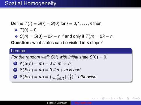
Spatial Homogeneity
Define T (i) = S(i)− S(0) for i = 0,1, . . . ,n thenT (0) = 0,S(n) = S(0) + 2k − n if and only if T (n) = 2k − n.
Question: what states can be visited in n steps?
LemmaFor the random walk S(i) with initial state S(0) = 0,
1 P (S(n) = m) = 0 if |m| > n,2 P (S(n) = m) = 0 if n + m is odd,3 P (S(n) = m) =
( n(n+m)/2
) (12
)n, otherwise.
J. Robert Buchanan Brownian Motion

Mean and Variance of Random Walk (1 of 2)
TheoremFor the random walk S(i) with initial state S(0) = 0,
E [S(n)] = 0 and Var (S(n)) = n.
J. Robert Buchanan Brownian Motion

Mean and Variance of Random Walk (2 of 2)
Proof.
E [S(n)] = E [S(0)] + E [X1] + E [X2] + · · ·+ E [Xn]
= 0
since E [Xi ] = 0 for i = 1,2, . . . ,n. If Xi and Xj are independentwhen i 6= j we have
Var (S(n)) = Var (S(0)) +n∑
i=1
Var (Xi) = n.
J. Robert Buchanan Brownian Motion

Reflections of Random Walks (1 of 2)
Consider a random walk for which S(k) = 0 for some k .
j
SH0L
A
-A
SHjL
J. Robert Buchanan Brownian Motion

Reflections of Random Walks (2 of 2)
If S(k) = 0 then define another random walk S(j) by
S(j) =
S(j) for j = 0,1, . . . , k−S(j) for j = k + 1, k + 2, . . . ,n.
Since UP/DOWN steps occur with equal probability,
P (S(n) = A) = P(
S(n) = −A).
J. Robert Buchanan Brownian Motion

Reflections of Random Walks (2 of 2)
If S(k) = 0 then define another random walk S(j) by
S(j) =
S(j) for j = 0,1, . . . , k−S(j) for j = k + 1, k + 2, . . . ,n.
Since UP/DOWN steps occur with equal probability,
P (S(n) = A) = P(
S(n) = −A).
J. Robert Buchanan Brownian Motion

Markov Property
Random walks have no “memory” of how they arrive at aparticular state. Only the current state influences the next state.
P (S(n) = A) = P(
S(n) = −A)
P (S(k) = 0) P (T (n − k) = A) = P(
S(k) = 0)
P(
T (n − k) = −A)
= P (S(k) = 0) P(
T (n − k) = −A)
P (T (n − k) = A) = P(
T (n − k) = −A)
J. Robert Buchanan Brownian Motion

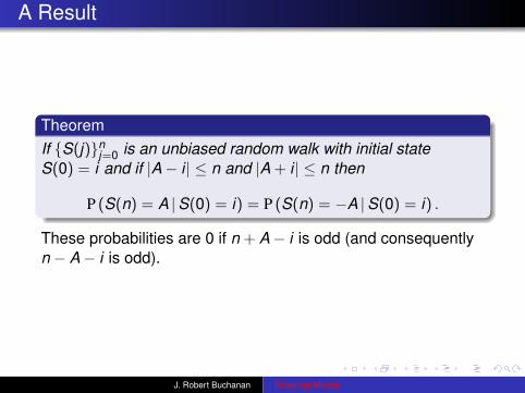
A Result
TheoremIf S(j)nj=0 is an unbiased random walk with initial stateS(0) = i and if |A− i | ≤ n and |A + i | ≤ n then
P (S(n) = A |S(0) = i) = P (S(n) = −A |S(0) = i) .
These probabilities are 0 if n + A− i is odd (and consequentlyn − A− i is odd).
J. Robert Buchanan Brownian Motion
A Result
TheoremIf S(j)nj=0 is an unbiased random walk with initial stateS(0) = i and if |A− i | ≤ n and |A + i | ≤ n then
P (S(n) = A |S(0) = i) = P (S(n) = −A |S(0) = i) .
These probabilities are 0 if n + A− i is odd (and consequentlyn − A− i is odd).
J. Robert Buchanan Brownian Motion

Absorbing Boundary Conditions
Remark: so far we have considered only random walks whichwere free to wander unrestricted.
What if there is a state A such that if S(k) = A then S(n) = Afor all n ≥ k? Such a state is called an absorbing boundarycondition.
ExampleA gambler going broke and unable to borrow money hasencountered an absorbing boundary condition.
J. Robert Buchanan Brownian Motion
Questions
Suppose random walk S(i) has an absorbing boundarycondition at 0. If 0 < S(0) < A,
1 what is the probability that the state of the random walkcrosses the threshold value of A before it hits the boundaryat 0?
2 what is the expected value of the number of steps whichwill elapse before the state of the random variable firstcrosses the A threshold?
J. Robert Buchanan Brownian Motion

Answer to First Question (1 of 2)
Define Smin(n) = minS(k) : 0 ≤ k ≤ n which can be thoughtof as the smallest value the random walk takes on.
The probability the state of the random walk crosses thethreshold value of A before it hits the boundary at 0 is then
P (S(n) = A ∧ Smin(n) > 0 |S(0) = i) .
J. Robert Buchanan Brownian Motion

Answer to First Question (2 of 2)
Lemma
Suppose a random walk S(k) = S(0) +∑k
i=1 Xi in which the Xifor i = 1,2, . . . are independent, identically distributed randomvariables taking on the values ±1, each with probabilityp = 1/2. Suppose further that the boundary at 0 is absorbing,then if A, i > 0,
fA,i(n) = P (S(n) = A ∧ Smin(n) > 0 |S(0) = i)
=
[(n
(n + A− i)/2
)−(
n(n − A− i)/2
)](12
)n
,
provided |A− i | ≤ n, |A + i | ≤ n, and n + A− i is even.
J. Robert Buchanan Brownian Motion

Proof (1 of 3)
Consider a random walk with no boundary, that is, the randomvariable S(n) has an initial state of S(0) = i > 0 and S(k) isallowed to wander into negative territory (and back) arbitrarily.In this situation
P (S(n) = A |S(0) = i)= P (S(n) = A ∧ Smin(n) > 0 |S(0) = i)
+ P (S(n) = A ∧ Smin(n) ≤ 0 |S(0) = i)
by the Addition Rule.
J. Robert Buchanan Brownian Motion

Proof (2 of 3)
Now consider the probability on the left-hand side of theequation.
P (S(n) = A |S(0) = i)
It possesses no boundary condition and by the spatialhomogeneity of the random walk
P (S(n) = A |S(0) = i) = P (T (n) = A− i)
where T (j)nj=0 is an unbiased random walk with initial stateT (0) = 0. Hence P (T (n) = A− i) = 0 unless n + A− i is evenand |A− i | ≤ n, in which case
P (S(n) = A |S(0) = i) =
(n
(n + A− i)/2
)(12
)n
.
J. Robert Buchanan Brownian Motion

Proof (3 of 3)
On the other hand if the random walk starts at a positive state iand finishes at −A < 0 then it is certain that Smin(n) ≤ 0.Consequently
P (S(n) = A ∧ Smin(n) ≤ 0 |S(0) = i) = P (S(n) = −A |S(0) = i)
=
(n
(n − A− i)/2
)(12
)n
provided |A + i | ≤ n and n − A− i is even. Finally
P (S(n) = A ∧ Smin(n) > 0 |S(0) = i)
=
(n
(n + A− i)/2
)(12
)n
−(
n(n − A− i)/2
)(12
)n
.
J. Robert Buchanan Brownian Motion

Example
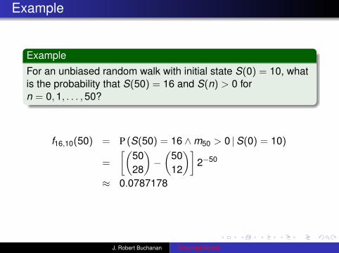
Example
For an unbiased random walk with initial state S(0) = 10, whatis the probability that S(50) = 16 and S(n) > 0 forn = 0,1, . . . ,50?
f16,10(50) = P (S(50) = 16 ∧m50 > 0 |S(0) = 10)
=
[(5028
)−(
5012
)]2−50
≈ 0.0787178
J. Robert Buchanan Brownian Motion
Example
Example
For an unbiased random walk with initial state S(0) = 10, whatis the probability that S(50) = 16 and S(n) > 0 forn = 0,1, . . . ,50?
f16,10(50) = P (S(50) = 16 ∧m50 > 0 |S(0) = 10)
=
[(5028
)−(
5012
)]2−50
≈ 0.0787178
J. Robert Buchanan Brownian Motion

Stopping Times
Define ΩA = minn |S(n) = A which is the first time that therandom walk S(n) = A. This is called the stopping time.
Suppose A = 0, then Ω0 = n if and only if S(0) = i > 0,S(n − 1) = 1, mn−1 > 0 and Xn = −1.
P (Ω0 = n |S(0) = i)= P (Xn = −1 ∧ S(n − 1) = 1 ∧mn−1 > 0 |S(0) = i)
=12
P (S(n − 1) = 1 ∧mn−1 > 0 |S(0) = i)
=12
f1,i(n − 1).
Thus by spatial homogeneity
P (ΩA = n |S(0) = i) =12
f1,(i−A)(n − 1)
J. Robert Buchanan Brownian Motion

Paths
We can analyze the stopping time by think of the random walkas having two boundaries, one at 0 and another at A.
pi→A: any random walk S(j) in the discrete interval[0,A] starting at i > 0, terminating at A, and whichavoids 0.
Ppi→A : the probability that the random walk starting atS(0) = i follows pi→A.
PA(i): the probability that a random walk which starts atS(0) = i will achieve state S = A while avoidingthe state S = 0.
J. Robert Buchanan Brownian Motion

Determination of PA(i)
PA(i) =∑pi→A
Ppi→A
= P (S(1) = i − 1 |S(0) = i)PA(i − 1)
+ P (S(1) = i + 1 |S(0) = i)PA(i + 1)
=12PA(i − 1) +
12PA(i + 1)
This implies
PA(i − 1)− 2PA(i) + PA(i + 1) = 0.
J. Robert Buchanan Brownian Motion

Determination of PA(i)
PA(i) =∑pi→A
Ppi→A
= P (S(1) = i − 1 |S(0) = i)PA(i − 1)
+ P (S(1) = i + 1 |S(0) = i)PA(i + 1)
=12PA(i − 1) +
12PA(i + 1)
This implies
PA(i − 1)− 2PA(i) + PA(i + 1) = 0.
J. Robert Buchanan Brownian Motion

Probability of Exiting
Theorem
Suppose S(k) = S(0) +∑k
i=1 Xi where the Xi for i = 1,2, . . .are independent, identically distributed random variables takingon the values ±1, each with probability p = 1/2. Supposefurther that the boundaries at 0 and A are absorbing, then if0 ≤ S(0) = i ≤ A
1 the probability that the random walk achieves state Awithout achieving state 0 is PA(i) = i/A,
2 the probability that the random walk achieves state 0without achieving state A is P0(i) = 1− i/A.
J. Robert Buchanan Brownian Motion

Proof
Suppose PA(i) = α + βi where α and β are constants.Substituting into the difference equation yields
α + β(i − 1)− 2(α + βi) + α + β(i + 1) = 0
so PA(i) solves the difference equation.
Since PA(0) = 0, then α = 0.
Since PA(A) = 1, then β = 1/A.
Consequently PA(i) = i/A.
J. Robert Buchanan Brownian Motion

Simpler Question
Question: what is the expected exit time through eitherboundary A > 0 or 0?
We make the following definitions:B: the set of boundary points, B = 0,A.
ωpi→B : the exit time of the random walk which starts atS(0) = i , where 0 ≤ i ≤ A and which follows pathpi→B.
ΩB(i): the expected value of the exit time for a randomwalk which starts at S(0) = i , where 0 ≤ i ≤ A.
J. Robert Buchanan Brownian Motion
Simpler Question
Question: what is the expected exit time through eitherboundary A > 0 or 0?We make the following definitions:
B: the set of boundary points, B = 0,A.ωpi→B : the exit time of the random walk which starts at
S(0) = i , where 0 ≤ i ≤ A and which follows pathpi→B.
ΩB(i): the expected value of the exit time for a randomwalk which starts at S(0) = i , where 0 ≤ i ≤ A.
J. Robert Buchanan Brownian Motion
Simple Answer
ΩB(i) =∑pi→B
Ppi→Bωpi→B
=12
(1 + ΩB(i − 1)) +12
(1 + ΩB(i + 1))
Since the path from i → B can be decomposed into paths from(i − 1)→ B and (i + 1)→ B with the addition of a single step,the expected value of the exit time of a random walk starting ati is one more than the expected value of a random walk startingat i ± 1.
J. Robert Buchanan Brownian Motion

System of Equations
ΩB(i − 1)− 2ΩB(i) + ΩB(i + 1) = −2
for i = 1,2, . . . ,A− 1, while ΩB(0) = 0 = ΩB(A).
Try a solution of the form ΩB(i) = ai2 + bi + c and determinethe coefficients a, b, and c.
J. Robert Buchanan Brownian Motion

System of Equations
ΩB(i − 1)− 2ΩB(i) + ΩB(i + 1) = −2
for i = 1,2, . . . ,A− 1, while ΩB(0) = 0 = ΩB(A).
Try a solution of the form ΩB(i) = ai2 + bi + c and determinethe coefficients a, b, and c.
J. Robert Buchanan Brownian Motion

A Result
Theorem
Suppose S(k) = S(0) +∑k
i=1 Xi where the Xi for i = 1,2, . . .are independent, identically distributed random variables takingon the values ±1, each with probability p = 1/2. Supposefurther that the boundaries at 0 and A are absorbing, then if0 ≤ S(0) = i ≤ A the random walk intersects the boundary(S = 0 or S = A) after a mean number of steps given by theformula
ΩB(i) = i(A− i).
J. Robert Buchanan Brownian Motion

Example
ExampleSuppose an unbiased random walk takes place on the discreteinterval 0,1,2, . . . ,10 for which the boundaries at 0 and 10are absorbing. As a function of the initial condition i , find theexpected value of the exit time.
i 0 1 2 3 4 5 6 7 8 9 10ΩB(i) 0 9 16 21 24 25 24 21 16 9 0
J. Robert Buchanan Brownian Motion

Main Question: Conditional Exit Time
Remark: now we are in a position to answer the originalquestion of the determining the expected value of the exit timefor a random walk which exits through state A while avoidingthe absorbing boundary at 0.
ΩA(i) =
∑pi→A
Ppi→Aωpi→A∑pi→A
Ppi→A
=
∑pi→A
Ppi→Aωpi→A
PA(i)
J. Robert Buchanan Brownian Motion

Decomposing the Walk (1 of 2)
ΩA(i) = 1 +12ΩA(i − 1)PA(i − 1) + 1
2ΩA(i + 1)PA(i + 1)
PA(i)
= PA(i) +12
ΩA(i − 1)PA(i − 1) +12
ΩA(i + 1)PA(i + 1)
ΩA(i)iA
=iA
+i − 12A
ΩA(i − 1) +i + 12A
ΩA(i + 1)
2iΩA(i) = 2i + (i − 1)ΩA(i − 1) + (i + 1)ΩA(i + 1)
J. Robert Buchanan Brownian Motion

Decomposing the Walk (2 of 2)
The last equation is equivalent to
(i − 1)ΩA(i − 1)− 2iΩA(i) + (i + 1)ΩA(i + 1) = −2i .
Assuming ΩA(i) = ai2 + bi + c, determine the coefficients a, b,and c.
J. Robert Buchanan Brownian Motion

Decomposing the Walk (2 of 2)
The last equation is equivalent to
(i − 1)ΩA(i − 1)− 2iΩA(i) + (i + 1)ΩA(i + 1) = −2i .
Assuming ΩA(i) = ai2 + bi + c, determine the coefficients a, b,and c.
J. Robert Buchanan Brownian Motion

Conditional Exit Time
Theorem
Suppose S(k) = S(0) +∑k
i=1 Xi where the Xi for i = 1,2, . . .are independent, identically distributed random variables takingon the values ±1, each with probability p = 1/2. Supposefurther that the boundary at 0 is absorbing. The random walkthat avoids state 0 will stop the first time that S(n) = A. Theexpected value of the stopping time is
ΩA(i) =13
(A2 − i2
), for i = 1,2, . . . ,A.
Remark: If the random walk starts in state 0, since this state isabsorbing the expected value of the exit time is infinity.
J. Robert Buchanan Brownian Motion

Example
ExampleSuppose an unbiased random walk takes place on the discreteinterval 0,1,2, . . . ,10 for which the boundary at 0 isabsorbing. As a function of the initial condition i , find theexpected value of the conditional exit time through state 10.
i 1 2 3 4 5 6 7 8 9 10Ω10(i) 33 32 91
3 28 25 643 17 12 19
3 0
J. Robert Buchanan Brownian Motion

Stochastic Processes
Now we begin the development of continuous random walks bytaking a limit of the previous discrete random walks.
Assumptions:S(0) = 0.n independent steps take place equally spaced in timeinterval [0, t ].Probability of a step to the left/right is 1/2.Size of a step is
√t/n.
Find E [S(t)] and Var (S(t)).
J. Robert Buchanan Brownian Motion

Stochastic Processes
Now we begin the development of continuous random walks bytaking a limit of the previous discrete random walks.Assumptions:
S(0) = 0.n independent steps take place equally spaced in timeinterval [0, t ].Probability of a step to the left/right is 1/2.Size of a step is
√t/n.
Find E [S(t)] and Var (S(t)).
J. Robert Buchanan Brownian Motion

Illustration
tk
SHkL
J. Robert Buchanan Brownian Motion

Brownian Motion/Wiener Process
The continuous limit of this random walk is denoted W (t) and iscalled a Wiener process.
1 W (t) is a continuous function of t ,2 W (0) = 0 with probability one,3 Spatial homogeneity: if W0(t) represents a Wiener process
for which the initial state is 0 and if Wx (t) represents aWiener process for which the initial state is x , thenWx (t) = x + W0(t).
4 Markov property: for 0 < s < t the conditional distributionof W (t) depends on the value of W (s) + W (t − s).
5 For each t , W (t) is normally distributed with mean zeroand variance t ,
6 The changes in W in non-overlapping intervals of t areindependent random variables with means of zero andvariances equal to the lengths of the time intervals.
J. Robert Buchanan Brownian Motion

More Properties
Suppose 0 ≤ t1 < t2 and define ∆W[t1,t2] = W (t2)−W (t1).
Var(∆W[t1,t2]
)= E
[(W (t2)−W (t1))2
]− E [W (t2)−W (t1)]2
= E[(W (t2))2
]+ E
[(W (t1))2
]− 2E [W (t1)W (t2)]
= t2 + t1 − 2E [W (t1)(W (t2)−W (t1) + W (t1))]
= t2 + t1 − 2E [W (t1)(W (t2)−W (t1))]
− 2E[(W (t1))2
]= t2 + t1 − 2t1= t2 − t1.
J. Robert Buchanan Brownian Motion

Differential Wiener Process
We have seen that for 0 ≤ t1 < t2,
Var (∆W ) = E[(∆W )2
]= ∆t .
This is also true in the limit as ∆t becomes small, thus we write
(dW (t))2 = dt .
TheoremThe derivative dW/dt does not exist for any t.
J. Robert Buchanan Brownian Motion

Differential Wiener Process
We have seen that for 0 ≤ t1 < t2,
Var (∆W ) = E[(∆W )2
]= ∆t .
This is also true in the limit as ∆t becomes small, thus we write
(dW (t))2 = dt .
TheoremThe derivative dW/dt does not exist for any t.
J. Robert Buchanan Brownian Motion

Proof
Recall the limit definition of the derivative from calculus,
dfdt
= limh→0
f (s + h)− f (s)
h.
Suppose f (t) is a Wiener process W (t). Since
E[(W (s + h)−W (s))2
]= E
[|W (s + h)−W (s)|2
]= h
then on average |W (s + h)−W (s)| ≈√
h, and therefore
limh→0
W (s + h)−W (s)
hdoes not exist.
J. Robert Buchanan Brownian Motion

Integral of a Wiener Process
The stochastic integral of f (x) on the interval [0, t ] is definedto be
Z (t)− Z (0) =
∫ t
0f (τ) dW (τ)
= limn→∞
n∑k=1
f (tk−1) (W (tk )−W (tk−1))
where tk = kt/n.
Note: The function f is evaluated at the left-hand endpoint ofeach subinterval.
The stochastic integral is equivalent to its differential form
dZ = f (t) dW (t)
J. Robert Buchanan Brownian Motion

ODE: Exponential Growth
If P(0) = P0 and the rate of change of P is proportional to P,then
dPdt
= µP,
and P(t) = P0eµt .
If we let Z = ln P then the ODE becomes
dZ = µdt .
J. Robert Buchanan Brownian Motion

ODE: Exponential Growth
If P(0) = P0 and the rate of change of P is proportional to P,then
dPdt
= µP,
and P(t) = P0eµt .
If we let Z = ln P then the ODE becomes
dZ = µdt .
J. Robert Buchanan Brownian Motion

Stochastic Differential Equation (SDE)
Perturb dZ by adding a Wiener process with mean zero andstandard deviation σ
√dt .
dZ = µdt + σ dW (t)
This is a generalized Wiener process. The constant µ iscalled the drift and the constant σ is called the volatility. Thesolution to the SDE is
Z (t) = Z (0) + µt +
∫ t
0σ dW (τ).
J. Robert Buchanan Brownian Motion

Expectation and Variance
E [Z (t)− Z (0)] = µtVar (Z (t)− Z (0)) = σ2t
In terms of numerical approximation,∫ t
0dW (τ) ≈
n∑j=1
Xj
where Xj is a normal random variable with mean 0 andvariance t/n.
J. Robert Buchanan Brownian Motion

Expectation and Variance
E [Z (t)− Z (0)] = µtVar (Z (t)− Z (0)) = σ2t
In terms of numerical approximation,∫ t
0dW (τ) ≈
n∑j=1
Xj
where Xj is a normal random variable with mean 0 andvariance t/n.
J. Robert Buchanan Brownian Motion

Example
ExampleSuppose the drift parameter is µ = 1 and the volatility isσ = 1/4, then the expected value of the Wiener process is tand the standard deviation is
√t/4.
0.2 0.4 0.6 0.8 1.0t
0.2
0.4
0.6
0.8
1.0
1.2
ZHtL
J. Robert Buchanan Brownian Motion

Example
Example
Suppose the drift parameter is µ = 1/4 and the volatility isσ = 1, then the expected value of the Wiener process is t/4and the standard deviation is
√t .
0.2 0.4 0.6 0.8 1.0t
-0.5
0.5
1.0
ZHtL
J. Robert Buchanan Brownian Motion
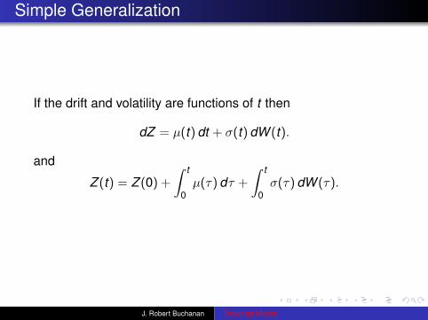
Simple Generalization
If the drift and volatility are functions of t then
dZ = µ(t) dt + σ(t) dW (t).
and
Z (t) = Z (0) +
∫ t
0µ(τ) dτ +
∫ t
0σ(τ) dW (τ).
J. Robert Buchanan Brownian Motion

Itô Processes
A stochastic process of the form
dS = a(S, t) dt + b(S, t) dW (t)
is called an Itô process.
We will shortly be called upon to develop new stochasticprocesses which are functions of S. Suppose Z = ln S, thendZ = dS/S (by the chain rule), but are the following twostochastic processes equivalent?
dS = µS dt + σS dW (t)dZ = µdt + σ dW (t)
J. Robert Buchanan Brownian Motion

Discussion
dS = µS dt + σS dW (t)dZ = µdt + σ dW (t)
µS → 0 and σS → 0 as S → 0+.
First equation makes a suitable mathematical model for astock price S ≥ 0, in second equation Z could go negative.Second equation can be integrated, first cannot.The two equations are not equivalent because the chainrule does not apply to functions of stochastic quantities.
J. Robert Buchanan Brownian Motion

Discussion
dS = µS dt + σS dW (t)dZ = µdt + σ dW (t)
µS → 0 and σS → 0 as S → 0+.First equation makes a suitable mathematical model for astock price S ≥ 0, in second equation Z could go negative.
Second equation can be integrated, first cannot.The two equations are not equivalent because the chainrule does not apply to functions of stochastic quantities.
J. Robert Buchanan Brownian Motion

Discussion
dS = µS dt + σS dW (t)dZ = µdt + σ dW (t)
µS → 0 and σS → 0 as S → 0+.First equation makes a suitable mathematical model for astock price S ≥ 0, in second equation Z could go negative.Second equation can be integrated, first cannot.
The two equations are not equivalent because the chainrule does not apply to functions of stochastic quantities.
J. Robert Buchanan Brownian Motion

Discussion
dS = µS dt + σS dW (t)dZ = µdt + σ dW (t)
µS → 0 and σS → 0 as S → 0+.First equation makes a suitable mathematical model for astock price S ≥ 0, in second equation Z could go negative.Second equation can be integrated, first cannot.The two equations are not equivalent because the chainrule does not apply to functions of stochastic quantities.
J. Robert Buchanan Brownian Motion

Itô’s Lemma
Lemma (Itô’s Lemma)Suppose that the random variable X is described by the Itôprocess
dX = a(X , t) dt + b(X , t) dW (t)
where dW (t) is a normal random variable. Suppose therandom variable Y = F (X , t). Then Y is described by thefollowing Itô process.
dY =
(a(X , t)FX + Ft +
12
(b(X , t))2FXX
)dt + b(X , t)FX dW (t)
J. Robert Buchanan Brownian Motion

Multivariable Form of Taylor’s Theorem (1 of 3)
If f (x) is an (n + 1)-times differentiable function on an openinterval containing x0 then the function may be written as
f (x) = f (x0) + f ′(x0)(x − x0) +f ′′(x0)
2!(x − x0)2 (1)
+ · · ·+ f (n)(x0)
n!(x − x0)n +
f (n+1)(θ)
(n + 1)!(x − x0)n+1
The last term above is usually called the Taylor remainderformula and is denoted by Rn+1. The quantity θ lies between xand x0. The other terms form a polynomial in x of degree atmost n and can be used as an approximation for f (x) in aneighborhood of x0.
J. Robert Buchanan Brownian Motion
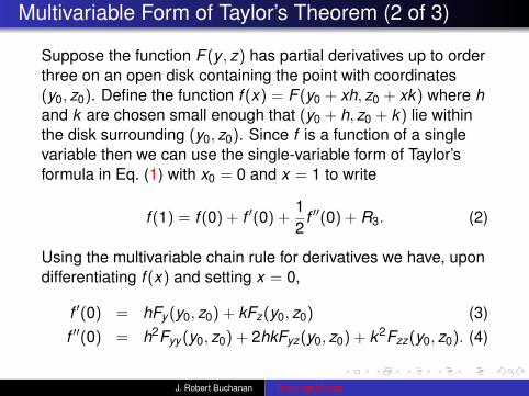
Multivariable Form of Taylor’s Theorem (2 of 3)
Suppose the function F (y , z) has partial derivatives up to orderthree on an open disk containing the point with coordinates(y0, z0). Define the function f (x) = F (y0 + xh, z0 + xk) where hand k are chosen small enough that (y0 + h, z0 + k) lie withinthe disk surrounding (y0, z0). Since f is a function of a singlevariable then we can use the single-variable form of Taylor’sformula in Eq. (1) with x0 = 0 and x = 1 to write
f (1) = f (0) + f ′(0) +12
f ′′(0) + R3. (2)
Using the multivariable chain rule for derivatives we have, upondifferentiating f (x) and setting x = 0,
f ′(0) = hFy (y0, z0) + kFz(y0, z0) (3)f ′′(0) = h2Fyy (y0, z0) + 2hkFyz(y0, z0) + k2Fzz(y0, z0). (4)
J. Robert Buchanan Brownian Motion

Multivariable Form of Taylor’s Theorem (3 of 3)
We have made use of the fact that Fyz = Fzy for this functionunder the smoothness assumptions. The remainder term R3contains only third order partial derivatives of F evaluatedsomewhere on the line connecting the points (y0, z0) and(y0 + h, z0 + k). Thus if we substitute Eqs. (3) and (4) into (2)we obtain
∆F = f (1)− f (0) (5)= F (y0 + h, z0 + k)− F (y0, z0)
= R3 + hFy (y0, z0) + kFz(y0, z0)
+12
(h2Fyy (y0, z0) + 2hkFyz(y0, z0) + k2Fzz(y0, z0)
).
This last equation can be used to derive Itô’s Lemma.
J. Robert Buchanan Brownian Motion

Proof (1 of 3)
Let X be a random variable described by an Itô process of theform
dX = a(X , t) dt + b(X , t) dW (t) (6)
where dW (t) is a normal random variable and a and b arefunctions of X and t . Let Y = F (X , t) be another randomvariable defined as a function of X and t . Given the Itô processwhich describes X we will now determine the Itô process whichdescribes Y .
J. Robert Buchanan Brownian Motion

Proof (2 of 3)
Using a Taylor series expansion for Y detailed in (5) we find
∆Y = FX ∆X + Ft ∆t +12
FXX (∆X )2 + FXt ∆X∆t
+12
Ftt (∆t)2 + R3
= FX (a∆t + b dW (t)) + Ft ∆t +12
FXX (a∆t + b dW (t))2
+ FXt (a∆t + b dW (t))∆t +12
Ftt (∆t)2 + R3.
J. Robert Buchanan Brownian Motion

Proof (3 of 3)
Upon simplifying, the expression ∆X has been replaced by thediscrete version of the Itô process. Thus as ∆t becomes small
∆Y ≈ FX (a dt + b dW (t)) + Ft dt +12!
FXX b2(dW (t))2.
Using the relationship (dW (t))2 = dt
∆Y ≈ FX (a dt + b dW (t)) + Ft dt +12!
FXX b2 dt . (7)
J. Robert Buchanan Brownian Motion

Examples (1 of 2)
ExampleIf Z = ln S and
dS = µS dt + σS dW (t),
find the stochastic process followed by Z .
If Z = ln S then
dZ =
(µS[
1S
]+ 0 +
12σ2S2
[− 1
S2
])dt + σS
(1S
)dW (t)
=
(µ− σ2
2
)dt + σ dW (t)
J. Robert Buchanan Brownian Motion

Examples (1 of 2)
ExampleIf Z = ln S and
dS = µS dt + σS dW (t),
find the stochastic process followed by Z .
If Z = ln S then
dZ =
(µS[
1S
]+ 0 +
12σ2S2
[− 1
S2
])dt + σS
(1S
)dW (t)
=
(µ− σ2
2
)dt + σ dW (t)
J. Robert Buchanan Brownian Motion

Examples (2 of 2)
Example
If S = eZ anddZ = µdt + σ dW (t),
find the stochastic process followed by S.
If S = eZ then
dS =
(µ[eZ]
+ 0 +12σ2[eZ])
dt + σ(
eZ)
dW (t)
=
(µ+
σ2
2
)S dt + σS dW (t)
J. Robert Buchanan Brownian Motion

Examples (2 of 2)
Example
If S = eZ anddZ = µdt + σ dW (t),
find the stochastic process followed by S.
If S = eZ then
dS =
(µ[eZ]
+ 0 +12σ2[eZ])
dt + σ(
eZ)
dW (t)
=
(µ+
σ2
2
)S dt + σS dW (t)
J. Robert Buchanan Brownian Motion

Stock Example (1 of 2)
Suppose we collect stock prices for n + 1 days:S(0),S(1), . . . ,S(n).
Under the lognormal assumption Z (i) = ln S(i + 1)/S(i) isa normal random variable.If the mean (drift) and variance (volatility squared) of Z areµ and σ2 respectively, then
dZ = µdt + σ dW (t).
J. Robert Buchanan Brownian Motion

Stock Example (1 of 2)
Suppose we collect stock prices for n + 1 days:S(0),S(1), . . . ,S(n).Under the lognormal assumption Z (i) = ln S(i + 1)/S(i) isa normal random variable.
If the mean (drift) and variance (volatility squared) of Z areµ and σ2 respectively, then
dZ = µdt + σ dW (t).
J. Robert Buchanan Brownian Motion

Stock Example (1 of 2)
Suppose we collect stock prices for n + 1 days:S(0),S(1), . . . ,S(n).Under the lognormal assumption Z (i) = ln S(i + 1)/S(i) isa normal random variable.If the mean (drift) and variance (volatility squared) of Z areµ and σ2 respectively, then
dZ = µdt + σ dW (t).
J. Robert Buchanan Brownian Motion

Stock Example (2 of 2)
Hence
Z (t) = Z (0) + µt +
∫ t
0σ dW (τ)
andS(t) = S(0)eµt+
R t0 σ dW (τ).
The mean and variance of S(t) are
E [S(t)] = S(0)e(µ+σ2/2)t
Var (S(t)) = (S(0))2e(2µ+σ2)t(
eσ2t − 1
).
J. Robert Buchanan Brownian Motion

Stock Example (2 of 2)
Hence
Z (t) = Z (0) + µt +
∫ t
0σ dW (τ)
andS(t) = S(0)eµt+
R t0 σ dW (τ).
The mean and variance of S(t) are
E [S(t)] = S(0)e(µ+σ2/2)t
Var (S(t)) = (S(0))2e(2µ+σ2)t(
eσ2t − 1
).
J. Robert Buchanan Brownian Motion


![Brownian Motion[1]](https://static.fdocuments.net/doc/165x107/577d35e21a28ab3a6b91ad47/brownian-motion1.jpg)