Yaglom-type limit theorems for

branching Brownian motion with absorption

by Jason Schweinsberg

University of California San Diego

(with Julien Berestycki, Nathanael Berestycki, Pascal Maillard)

Outline

1. Definition of the process

2. Main results

3. Proof techniques

4. Application to populations undergoing selection

Branching Brownian motion with absorption

Begin with some configuration of particles in (0,∞).

Each particle independently moves according to standard one-

dimensional Brownian motion with drift −µ.

Each particle splits into two particles at rate 1/2 (more general

supercritical offspring distributions can also be handled).

Particles are killed if they reach the origin.

time t

time 0 @@��

��@@��

@@��@@��

�� @@����

�� ���� ��

���

��@@���� @@��u u u

u

u

u

Condition for extinction

Theorem (Kesten, 1978): Branching Brownian motion with ab-

sorption dies out almost surely if µ ≥ 1. If µ < 1, the process

survives forever with positive probability.

Hereafter, we always assume µ = 1 (critical drift).

Questions

• What is the probability that the process survives until a large

time t?

• Conditional on survival until a large time t, what does the

configuration of particles look like at time t? (Such results

are known as Yaglom-type limit theorems.)

Long-run survival probability

Let N(t) be the number of particles at time t.

Let ζ = inf{t : N(t) = 0} be the extinction time.

Let c = (3π2/2)1/3.

Theorem (Kesten, 1978): There exists K > 0 such that foreach x > 0, we have for sufficiently large t:

xex−ct1/3−K(log t)2

≤ Px(ζ > t) ≤ (1 + x)ex−ct1/3+K(log t)2

.

Theorem (BMS, 2017): There is a positive constant C suchthat for all x > 0, we have as t→∞,

Px(ζ > t) ∼ Cxex−ct1/3.

Remark:

• Derrida and Simon (2007) obtained result nonrigorously.

• The weaker bound C1xex−ct1/3 ≤ Px(ζ > t) ≤ C2xe

x−ct1/3was

obtained by BBS (2014).

The process conditioned on survival

Let N(t) be the number of particles at time t.

Let R(t) be the position of the right-most particle at time t.

Theorem (Kesten, 1978): There are positive constants K1 and

K2 such that for all x > 0,

limt→∞

Px(N(t) > eK1t2/9(log t)2/3

| ζ > t) = 0

limt→∞

Px(R(t) > K2t2/9(log t)2/3 | ζ > t) = 0.

Theorem (BMS, 2017): If the process starts with one particle

at x > 0, then conditional on survival until time t,

t−2/9 logN(t)⇒ V 1/3

t−2/9R(t)⇒ V 1/3,

where V has an exponential distribution with mean 3c2.

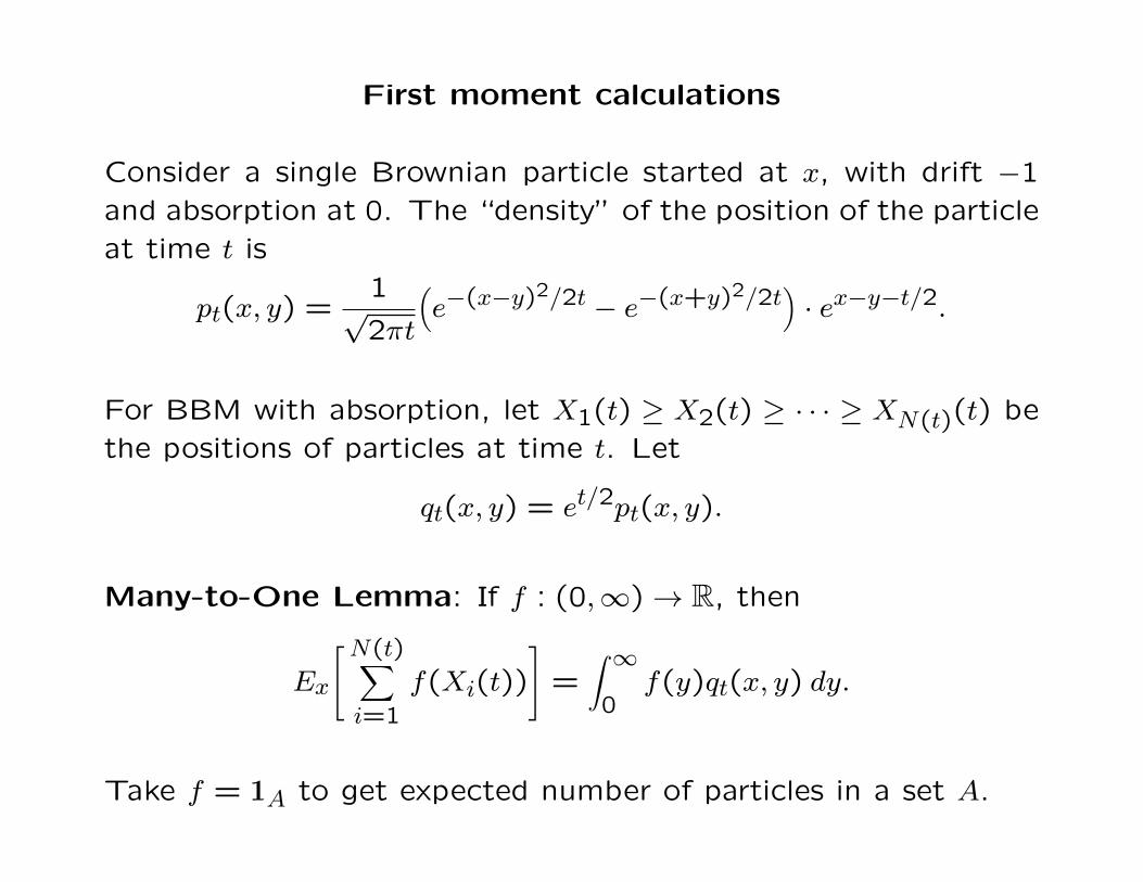
First moment calculations

Consider a single Brownian particle started at x, with drift −1and absorption at 0. The “density” of the position of the particleat time t is

pt(x, y) =1√2πt

(e−(x−y)2/2t − e−(x+y)2/2t

)· ex−y−t/2.

For BBM with absorption, let X1(t) ≥ X2(t) ≥ · · · ≥ XN(t)(t) bethe positions of particles at time t. Let

qt(x, y) = et/2pt(x, y).

Many-to-One Lemma: If f : (0,∞)→ R, then

Ex

[N(t)∑i=1

f(Xi(t))

]=∫ ∞

0f(y)qt(x, y) dy.

Take f = 1A to get expected number of particles in a set A.

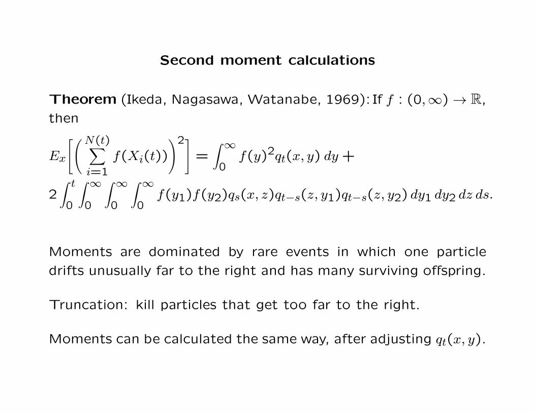
Second moment calculations

Theorem (Ikeda, Nagasawa, Watanabe, 1969): If f : (0,∞)→ R,

then

Ex

[(N(t)∑i=1

f(Xi(t))

)2]=∫ ∞

0f(y)2qt(x, y) dy +

2∫ t

0

∫ ∞0

∫ ∞0

∫ ∞0

f(y1)f(y2)qs(x, z)qt−s(z, y1)qt−s(z, y2) dy1 dy2 dz ds.

Moments are dominated by rare events in which one particle

drifts unusually far to the right and has many surviving offspring.

Truncation: kill particles that get too far to the right.

Moments can be calculated the same way, after adjusting qt(x, y).

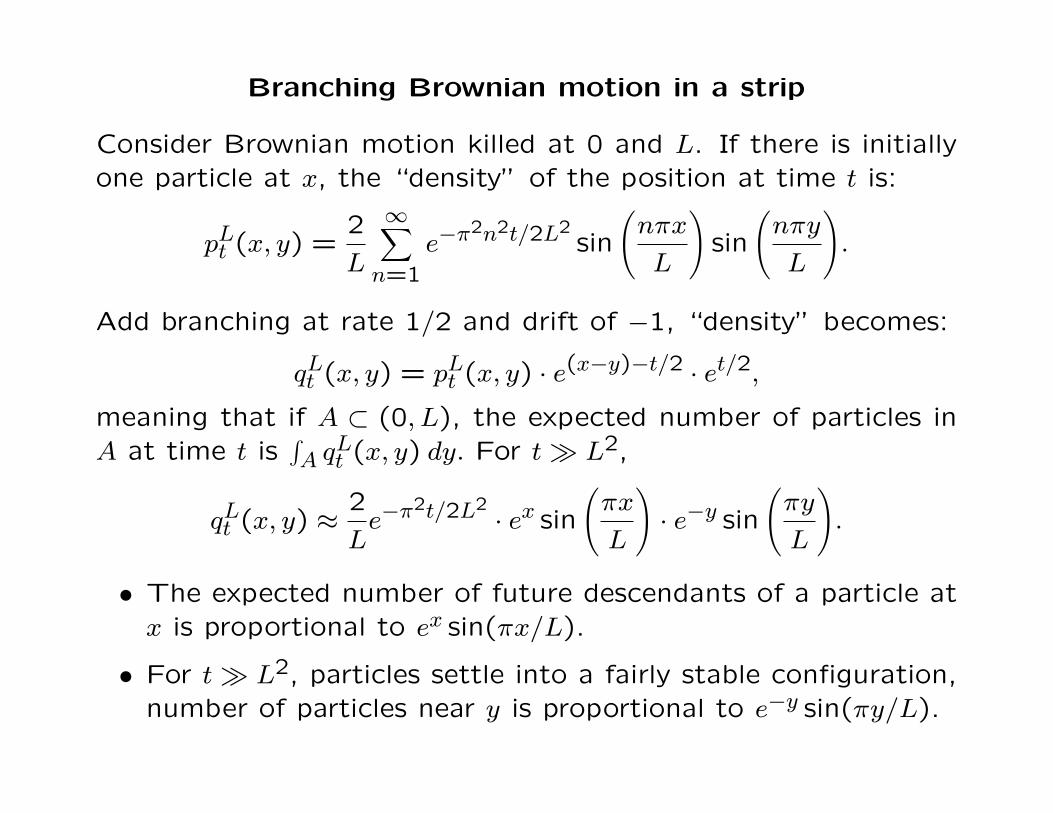
Branching Brownian motion in a strip

Consider Brownian motion killed at 0 and L. If there is initiallyone particle at x, the “density” of the position at time t is:

pLt (x, y) =2

L

∞∑n=1

e−π2n2t/2L2

sin

(nπx

L

)sin

(nπy

L

).

Add branching at rate 1/2 and drift of −1, “density” becomes:

qLt (x, y) = pLt (x, y) · e(x−y)−t/2 · et/2,

meaning that if A ⊂ (0, L), the expected number of particles inA at time t is

∫A q

Lt (x, y) dy. For t� L2,

qLt (x, y) ≈2

Le−π

2t/2L2· ex sin

(πx

L

)· e−y sin

(πy

L

).

• The expected number of future descendants of a particle atx is proportional to ex sin(πx/L).

• For t� L2, particles settle into a fairly stable configuration,number of particles near y is proportional to e−y sin(πy/L).

A curved right boundary

Fix t > 0. Let Lt(s) = c(t− s)1/3, where c = (3π2/2)1/3.Consider BBM with particles killed at 0 and Lt(s).This right boundary was previously used by Kesten (1978).

Roughly, a particle that gets within a constant of Lt(s) at times has a good chance to have a descendant alive at time t.

time 0

time t

s 7→ Lt(s)

u

uuuuuuuuuuuuuuuuuuuuuuuuuuuuuuuuuuuuuuuuuuuuuuuuuuuuuuuuuuuuuuuuuuuuuuuuuuUse methods of Novikov (1981) and Roberts (2012) toapproximate the density and then compute moments.

Density formula resembles that for BBM in a strip.

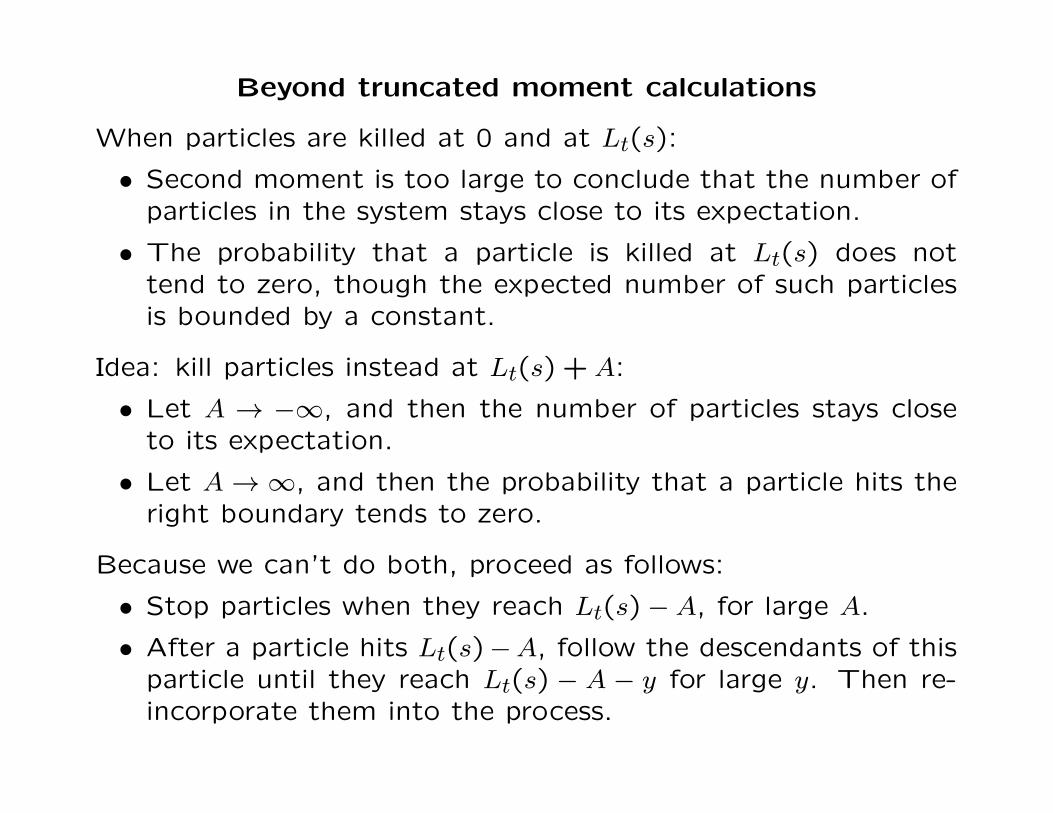
Beyond truncated moment calculations

When particles are killed at 0 and at Lt(s):

• Second moment is too large to conclude that the number ofparticles in the system stays close to its expectation.

• The probability that a particle is killed at Lt(s) does nottend to zero, though the expected number of such particlesis bounded by a constant.

Idea: kill particles instead at Lt(s) +A:

• Let A → −∞, and then the number of particles stays closeto its expectation.

• Let A→∞, and then the probability that a particle hits theright boundary tends to zero.

Because we can’t do both, proceed as follows:

• Stop particles when they reach Lt(s)−A, for large A.

• After a particle hits Lt(s)−A, follow the descendants of thisparticle until they reach Lt(s) − A − y for large y. Then re-incorporate them into the process.

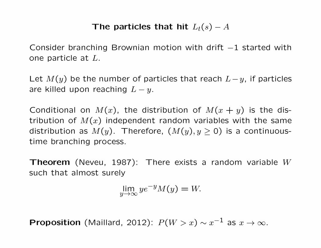
The particles that hit Lt(s)−A

Consider branching Brownian motion with drift −1 started withone particle at L.

Let M(y) be the number of particles that reach L−y, if particlesare killed upon reaching L− y.

Conditional on M(x), the distribution of M(x + y) is the dis-tribution of M(x) independent random variables with the samedistribution as M(y). Therefore, (M(y), y ≥ 0) is a continuous-time branching process.

Theorem (Neveu, 1987): There exists a random variable W

such that almost surely

limy→∞ ye

−yM(y) = W.

Proposition (Maillard, 2012): P (W > x) ∼ x−1 as x→∞.

Putting the pieces together

Consider BBM with drift at rate -1, branching at rate 1/2, andabsorption at 0.

Let N(s) be the number of particles at time s.

Let X1(s) ≥ X2(s) ≥ · · · ≥ XN(s)(s) be the positions of theparticles at time s.

Let t > 0. For 0 ≤ s ≤ t, let

Zt(s) =N(s)∑i=1

Lt(s)eXi(s)−Lt(s) sin

(πXi(s)

Lt(s)

)1{0<Xi(s)<Lt(s)}.

The processes (Zt(s),0 ≤ s ≤ t) converge as t→∞:

• The limit process has jumps of size greater than x at a rateproportional to x−1.

• The jump rate at time s is also proportional to Zt(s).

Limit is a continuous-state branching process.

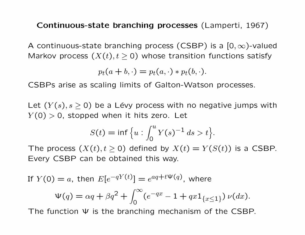
Continuous-state branching processes (Lamperti, 1967)

A continuous-state branching process (CSBP) is a [0,∞)-valuedMarkov process (X(t), t ≥ 0) whose transition functions satisfy

pt(a+ b, ·) = pt(a, ·) ∗ pt(b, ·).

CSBPs arise as scaling limits of Galton-Watson processes.

Let (Y (s), s ≥ 0) be a Levy process with no negative jumps withY (0) > 0, stopped when it hits zero. Let

S(t) = inf{u :

∫ u0Y (s)−1 ds > t

}.

The process (X(t), t ≥ 0) defined by X(t) = Y (S(t)) is a CSBP.Every CSBP can be obtained this way.

If Y (0) = a, then E[e−qY (t)] = eaq+tΨ(q), where

Ψ(q) = αq + βq2 +∫ ∞

0(e−qx − 1 + qx1{x≤1}) ν(dx).

The function Ψ is the branching mechanism of the CSBP.

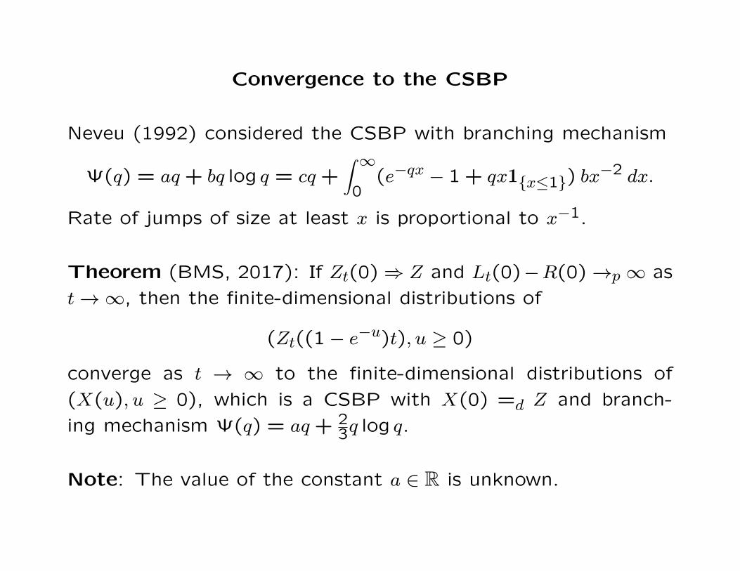
Convergence to the CSBP

Neveu (1992) considered the CSBP with branching mechanism

Ψ(q) = aq + bq log q = cq +∫ ∞

0(e−qx − 1 + qx1{x≤1}) bx

−2 dx.

Rate of jumps of size at least x is proportional to x−1.

Theorem (BMS, 2017): If Zt(0)⇒ Z and Lt(0)−R(0)→p ∞ as

t→∞, then the finite-dimensional distributions of

(Zt((1− e−u)t), u ≥ 0)

converge as t → ∞ to the finite-dimensional distributions of

(X(u), u ≥ 0), which is a CSBP with X(0) =d Z and branch-

ing mechanism Ψ(q) = aq + 23q log q.

Note: The value of the constant a ∈ R is unknown.

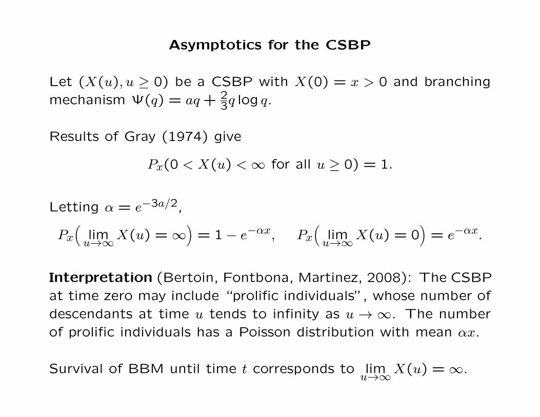
Asymptotics for the CSBP

Let (X(u), u ≥ 0) be a CSBP with X(0) = x > 0 and branching

mechanism Ψ(q) = aq + 23q log q.

Results of Gray (1974) give

Px(0 < X(u) <∞ for all u ≥ 0) = 1.

Letting α = e−3a/2,

Px(

limu→∞X(u) =∞

)= 1− e−αx, Px

(limu→∞X(u) = 0

)= e−αx.

Interpretation (Bertoin, Fontbona, Martinez, 2008): The CSBP

at time zero may include “prolific individuals”, whose number of

descendants at time u tends to infinity as u → ∞. The number

of prolific individuals has a Poisson distribution with mean αx.

Survival of BBM until time t corresponds to limu→∞X(u) =∞.

Survival probability for BBM

Theorem (BMS, 2017): Assume the initial configuration of par-ticles is deterministic, but may depend on t. Recall that ζ denotesthe extinction time.

• If Zt(0)→ z and Lt(0)−R(0)→∞ as t→∞, then

limt→∞

P (ζ > t) = 1− e−αz.

• If Zt(0)→ 0 and Lt(0)−R(0)→∞, then

P (ζ > t) ∼ αZt(0).

• If at time zero there is only a single particle at x, then

Px(ζ > t) ∼ απxex−Lt(0).

• If at time zero there is a single particle at Lt(0) + x, then

limt→∞

PLt(0)+x(ζ > t) = φ(x),

where limx→∞φ(x) = 1 and lim

x→−∞φ(x) = 0.

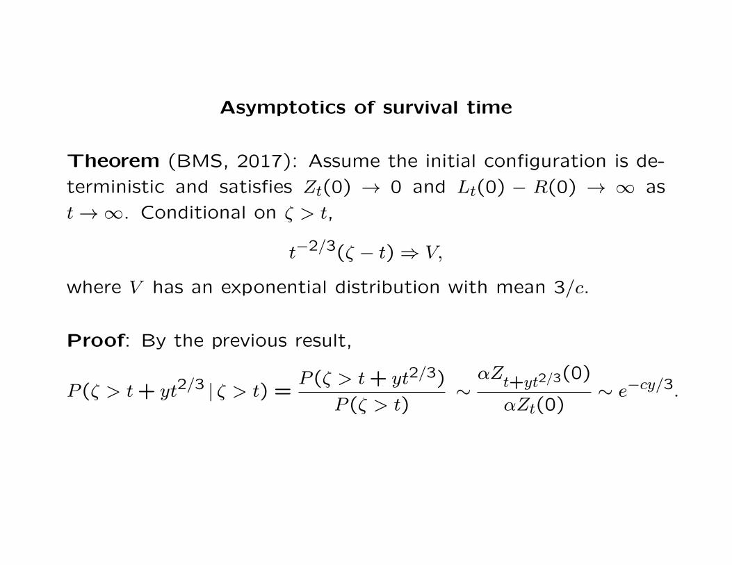
Asymptotics of survival time

Theorem (BMS, 2017): Assume the initial configuration is de-

terministic and satisfies Zt(0) → 0 and Lt(0) − R(0) → ∞ as

t→∞. Conditional on ζ > t,

t−2/3(ζ − t)⇒ V,

where V has an exponential distribution with mean 3/c.

Proof: By the previous result,

P (ζ > t+ yt2/3 | ζ > t) =P (ζ > t+ yt2/3)

P (ζ > t)∼αZ

t+yt2/3(0)

αZt(0)∼ e−cy/3.

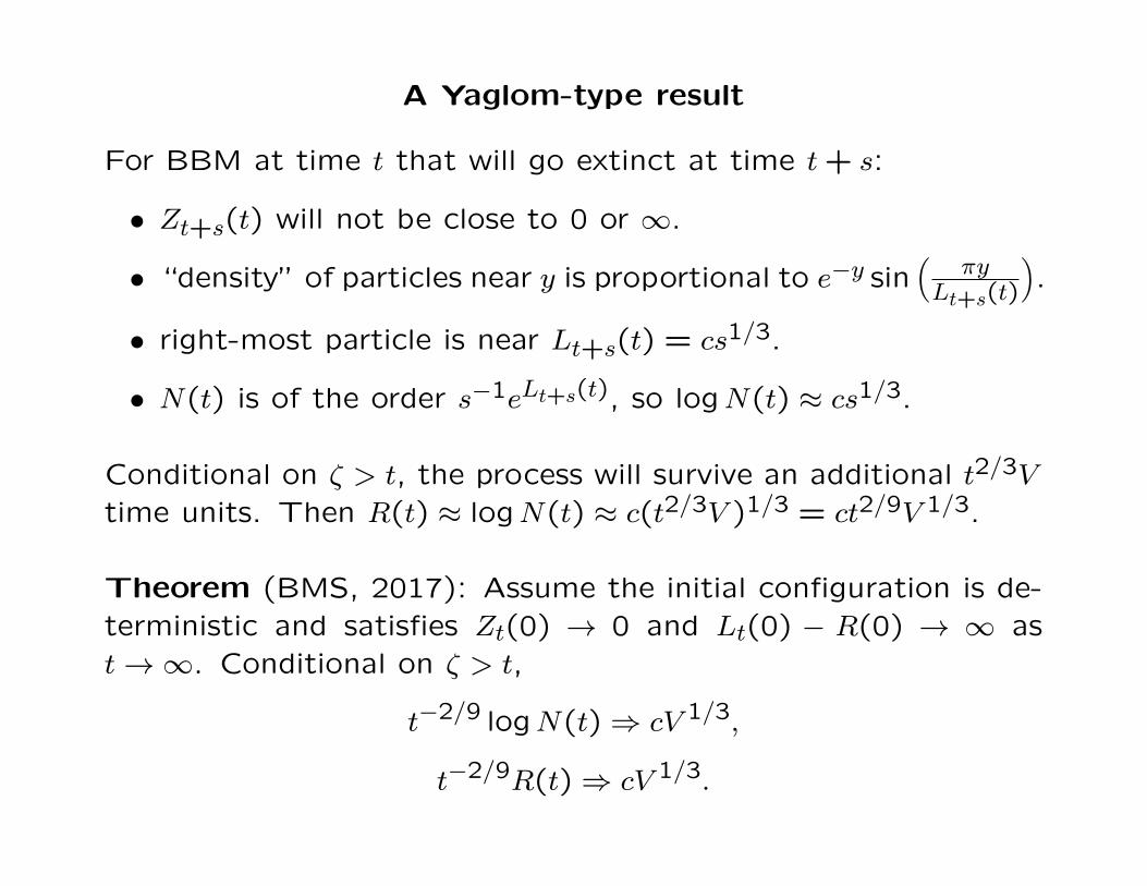
A Yaglom-type result

For BBM at time t that will go extinct at time t+ s:

• Zt+s(t) will not be close to 0 or ∞.

• “density” of particles near y is proportional to e−y sin(

πyLt+s(t)

).

• right-most particle is near Lt+s(t) = cs1/3.

• N(t) is of the order s−1eLt+s(t), so logN(t) ≈ cs1/3.

Conditional on ζ > t, the process will survive an additional t2/3V

time units. Then R(t) ≈ logN(t) ≈ c(t2/3V )1/3 = ct2/9V 1/3.

Theorem (BMS, 2017): Assume the initial configuration is de-terministic and satisfies Zt(0) → 0 and Lt(0) − R(0) → ∞ ast→∞. Conditional on ζ > t,

t−2/9 logN(t)⇒ cV 1/3,

t−2/9R(t)⇒ cV 1/3.

The conditioned BBM before time t

Theorem (BMS, 2017): Assume the initial configuration is de-

terministic and satisfies Zt(0) → 0 and Lt(0) − R(0) → ∞ as

t→∞. Conditional on ζ > t, the finite-dimensional distributions

of the processes

(Zt((1− e−u)t), u ≥ 0)

converge as t → ∞ to the finite-dimensional distributions of a

CSBP with branching mechanism Ψ(q) = aq+ 23q log q started at

0 and conditioned to go to infinity.

Remark: The law of the CSBP started at x > 0 and conditioned

to go to infinity has a limit as x→ 0. The limit can be interpreted

as the process that keeps track of the number of descendants of

a single prolific individual.

Population models with selection

Can use BBM with absorption to model populations subject to

natural selection, as proposed by Brunet, Derrida, Mueller, and

Munier (2006).

particles → individuals in the population

positions of particles → fitness of individuals

branching events → births

absorption at 0 → deaths of unfit individuals

movement of particles → changes in fitness over generations

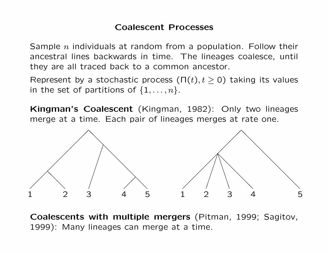
Coalescent Processes

Sample n individuals at random from a population. Follow theirancestral lines backwards in time. The lineages coalesce, untilthey are all traced back to a common ancestor.

Represent by a stochastic process (Π(t), t ≥ 0) taking its valuesin the set of partitions of {1, . . . , n}.

Kingman’s Coalescent (Kingman, 1982): Only two lineagesmerge at a time. Each pair of lineages merges at rate one.

���������������

@@@

@@@

@@@

@@@

@@@

@@

@@@

���

�����������

1 52 3 4���������������

@@

@@

@@@

@@@

@@@

@@

@@@@@@@@@

BBBBBBBBB

���������

1 52 3 4

Coalescents with multiple mergers (Pitman, 1999; Sagitov,1999): Many lineages can merge at a time.

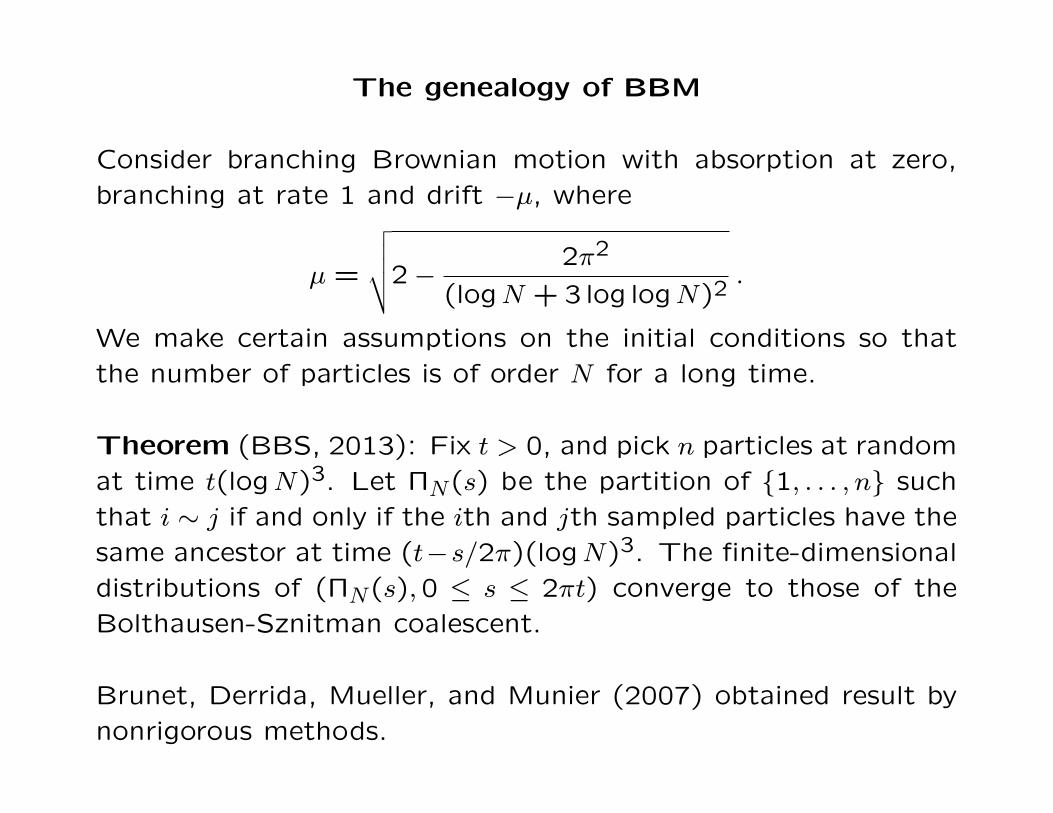
Bolthausen-Sznitman coalescent

When there are b lineages, each k-tuple (2 ≤ k ≤ b) of lineagesmerges at rate

λb,k =∫ 1

0pk−2(1− p)b−k dp.

Consider a Poisson point process on [0,∞)× (0,1] with intensity

dt× p−2 dp.

Begin with n lineages at time 0. If (t, p) is a point of this Poissonprocess, then at time t, there is a merger event in which eachlineage independently participates with probability p.

Rate of mergers impacting more than a fraction x/(1 + x) oflineages is ∫ 1

x/(1+x)p−2 dp = x−1.

Bolthausen-Sznitman coalescent describes the genealogy when,if the population has size K, new “families” of size at least Kxappear at a rate proportional to x−1. This applies to Neveu’sCSBP (Bertoin and Le Gall, 2000).

The genealogy of BBM

Consider branching Brownian motion with absorption at zero,

branching at rate 1 and drift −µ, where

µ =

√√√√2−2π2

(logN + 3 log logN)2.

We make certain assumptions on the initial conditions so that

the number of particles is of order N for a long time.

Theorem (BBS, 2013): Fix t > 0, and pick n particles at random

at time t(logN)3. Let ΠN(s) be the partition of {1, . . . , n} such

that i ∼ j if and only if the ith and jth sampled particles have the

same ancestor at time (t−s/2π)(logN)3. The finite-dimensional

distributions of (ΠN(s),0 ≤ s ≤ 2πt) converge to those of the

Bolthausen-Sznitman coalescent.

Brunet, Derrida, Mueller, and Munier (2007) obtained result by

nonrigorous methods.