Betriebswirtschaftliche Bewertungsmethoden Topic 3 Risk, Return, and The CAPM

slide no.: 1

Prof. Dr. Rainer StachuletzCorporate FinanceBerlin School of Economics

Betriebswirtschaftliche Bewertungsmethoden

Topic 3

Risk, Return, and The CAPM

Prof. Dr.Rainer StachuletzCorporate Finance

slide no.: 2


Topics Covered

• Who knows ???

slide no.: 3


Expected Returns

Decisions must be based on expected returns

Methods used to estimate expected return

Historical approach

Probabilistic approach

Risk-based approach

slide no.: 4


Historical ApproachExpected Returns

Assume that distribution of expected returns will be similar to historical distribution of returns.

Using 1900-2003 annual returns, the average risk premium for U.S. stocks relative to Treasury bills is 7.6%. Treasury

bills currently offer a 2% yield to maturity

Expected return on U.S. stocks: 7.6% + 2% = 9.6%

Can historical approach be used to estimate the expected return of an individual stock?

slide no.: 5


Historical Approach Expected Returns

Assume General Motors long-run average return is 17.0%. Treasury bills average return over

same period was 4.1%

GM historical risk premium: 17.0% - 4.1% = 12.9%

GM expected return = Current Tbill rate + GM historical risk premium = 2% + 12.9% = 14.9%

Limitations of historical

approach for individual

stocks

May reflect GM’s past more than its future

Many stocks have a long history to forecast expected return

slide no.: 6


Probabilistic Approach Expected Returns

Identify all possible outcomes of returns and assign a probability to each possible outcome:

GM Expected Return = 0.20(-30%) + 0.70(15%) +0.10(55%) = 10%

For example, assign probabilities for possible states of economy: boom, expansion, recession and project the

returns of GM stock for the three states

55%10%Boom

15%70%Expansion

-30%20%Recession

GM ReturnProbabilityOutcome

slide no.: 7


Risk-Based Approach

Expected Returns1. Measure the risk of the asset 2. Use the risk measure to estimate the

expected return

How can we capture the systematic risk component of a stock’s volatility?

1. Measure the risk of the asset

• Systematic risks simultaneously affect many different assets

• Investors can diversify away the unsystematic risk

• Market rewards only the systematic risk: only systematic risk should be related to the expected return

slide no.: 8


• Collect data on a stock’s returns and returns on a market index

• Plot the points on a scatter plot graph– Y–axis measures stock’s return– X-axis measures market’s return

• Plot a line (using linear regression) through the points

Risk-Based Approach Expected Returns

Slope of line equals beta, the sensitivity of a stock’s returns relative to changes in overall

market returns

Beta is a measure of systematic risk for a particular security.

slide no.: 9


Scatter Plot for Returns on Sharper Image and S&P 500

S&P 500 weekly returns

Sharp

er

Imag

e w

eekl

y r

etu

rns

slide no.: 10


Scatter Plot for Returns ConAgra and S&P 500

-15%

-10%

-5%

0%

5%

10%

15%

-15% -10% -5% 0% 5% 10% 15%

Beta = 0.11

S&P 500 weekly returns

ConA

gra

weekl

y r

etu

rns

slide no.: 11


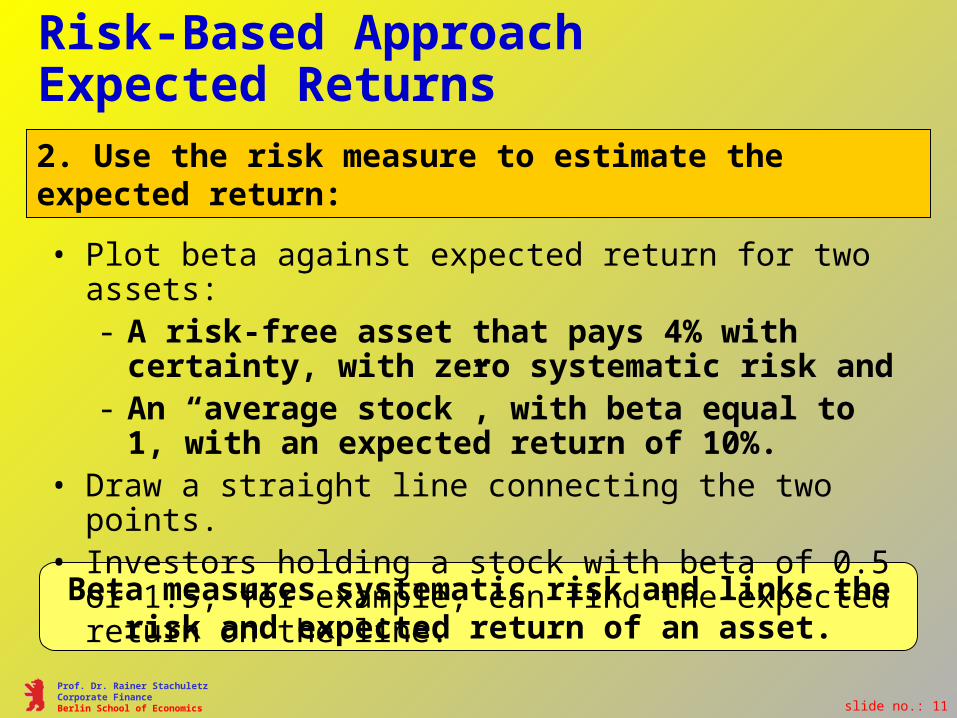
Risk-Based Approach Expected Returns

Beta measures systematic risk and links the risk and expected return of an asset.

2. Use the risk measure to estimate the expected return:

• Plot beta against expected return for two assets:- A risk-free asset that pays 4% with

certainty, with zero systematic risk and- An “average stock”, with beta equal to 1,

with an expected return of 10%.• Draw a straight line connecting the two points.• Investors holding a stock with beta of 0.5 or 1.5,

for example, can find the expected return on the line.

slide no.: 12


Risk and Expected Returns

What is the expected return for stock with beta = 1.5 ?

Expected returns

•

•10%

1

Risk-free asset

• • • •0.2 0.4 0.6 0.8 21.2 1.4 1.6 1.8

• • • • •

Beta

•4%

•18%

•14%

“average” stock

ß = 1.5•

•

slide no.: 13


Portfolio Expected Returns

The portfolio expected return equals the weighted average of the portfolio assets’

expected returns

E(Rp) = w1E(R1)+ w2E(R2)+…+wnE(Rn)• w1, w2 , … , wn : portfolio weights

• E(R1), E(R2), …, E(RN): expected returns of securities

Expected return of a portfolio with N securities

How does the expected return of a portfolio relate to the expected returns of the securities in the portfolio?

slide no.: 14


Portfolio Expected Returns

Portfolio

E(R) $ Invested Weights

IBM 10% $2,500 0.125

GE 12% $5,000 0.25

Sears 8% $2,500 0.125

Pfizer 14% $10,000 0.5

E (Rp) = (0.125) (10%) + (0.25) (12%) + (0.125) (8%) + (0.5) (14%) = 12.25%

E (Rp) = w1 E (R1)+ w2 E (R2)+…+wn E (Rn)

slide no.: 15


Portfolio RiskPortfolio risk is the weighted average of systematic risk (beta) of the portfolio constituent securities. Portfolio

Beta $ Invested Weights

IBM 1.00 $2,500 0.125

GE 1.33 $5,000 0.25

Sears 0.67 $2,500 0.125

Pfizer 1.67 $10,000 0.5ß P = (0.125) (1.00) + (0.25) (1.33) + (0.125) (0.67) + (0.50) (1.67) = 1.38But portfolio volatility is not the same as the weighted average of

all portfolio security volatilities

slide no.: 16


Security Market Line

Portfolio E(R) Beta

Risk-free asset Rf 0

Market portfolio E(Rm) 1

Portfolio composed of the following two assets:

• An asset that pays a risk-free return Rf, , and • A market portfolio that contains some of every

risky asset in the market.

Security market line: The line connecting the risk-free asset and the market portfolio

slide no.: 17


Security Market Line and CAPMThe two-asset portfolio lies on security market line

Given two points (risk-free asset and market portfolio asset) on the security market line, the

equation of the line:

E (Ri) = Rf + ß [E (Rm) – Rf]

• Return for bearing no market risk

• Portfolio’s exposure to market risk

• Reward for bearing market risk

The equation represents the risk and return relationship predicted by the Capital Asset Pricing

Model (CAPM)

slide no.: 18


The Security Market Line

• In equilibrium, all assets lie on this line.

• If individual stock or portfolio lies above the line:

•Expected return is too high.

• Investors bid up price until expected return falls.

• If individual stock or portfolio lies below SML:

•Expected return is too low.

• Investors sell stock driving down price until expected return rises.

Plots relationship between expected return and betas

slide no.: 19


The Security Market Line

i

E(RP)

RF

SML

Slope = E(Rm) - RF = Market Risk Premium

•A - Undervalued

•

•

•RM

=1.0

•B

•A

• B - Overvalued

slide no.: 20


Efficient Markets

Efficient market hypothesis (EMH): in an efficient market, prices rapidly incorporate all relevant

information

Financial markets much larger, more competitive, more transparent, more homogeneous than product

markets

Much harder to create value through financial activities

Changes in asset price respond only to new information. This implies that asset prices move

almost randomly.

slide no.: 21


Efficient Markets

CAPM gives analyst a model to measure the systematic risk of any asset.

If asset prices unpredictable, then what is the use of CAPM?

On average, assets with high systematic risk should earn higher returns than assets with

low systematic risk.

CAPM offers a way to compare risk and return on investments alternatives.

slide no.: 22


• Decisions should be made based on expected returns.

• Expected returns can be estimated using historical, probabilistic, or risk approaches.

• Portfolio expected return/beta equals weighted average of the expected returns/beta of the assets in the portfolio.

• CAPM predicts that the expected return on a stock depends on the stock’s beta, the risk-free rate and the market premium.

Risk, Return, and CAPM

Betriebswirtschaftliche Bewertungsmethoden Topic 3 Risk, Return, and The CAPM

Documents

Transcript of Betriebswirtschaftliche Bewertungsmethoden Topic 3 Risk, Return, and The CAPM