Approaches to Resolving and Tracking Interfaces and Discontinuties
30
Naval Research Laboratory • F•f• cljpy Washington, DC 20375.5000 NRL Memorandum Report 5999 00 Approaches to Resolving and Tracking Interfaces and Discontinuties I 0 K. J. LASKEY*, E. S. ORAN AND J. P. BORIS Laboratory for ComputationalPhysics and Fluid Dynamics *Berkley Research Associates, Inc. P.O. Box 852 Springfield, VA 22150 July 28, 1987 S AG 2 1 19 8 7u 87 Approved for public release; distribution unlimited.
Transcript of Approaches to Resolving and Tracking Interfaces and Discontinuties
Naval Research Laboratory • F•f• cljpyWashington, DC 20375.5000
NRL Memorandum Report 5999
00
Approaches to Resolving and TrackingInterfaces and DiscontinutiesI
0 K. J. LASKEY*, E. S. ORAN AND J. P. BORIS
Laboratory for Computational Physics
and Fluid Dynamics
*Berkley Research Associates, Inc.
P.O. Box 852Springfield, VA 22150
July 28, 1987
S AG 2 1 19 87u
87 Approved for public release; distribution unlimited.
SECURITY " OF TIPA
REPORT DOCUMENTATION PAGEli. REPORT SECURITY CLASSIFICATION lb. RESTRICTIVE MARKINGS
UNCLASSIFIED2a. SECURITY CLASSIFICATION AUTHORITY 3 DISTRIBUTION/AVAILABILITY OF REPORT
Approved for public release; distribution2b. DECLASSIFICATION IFDOWNGRADING SCHEDULE ulmtdunlimited.
4. PERFORMING ORGANIZATION REPORT NUMBER(S) 5. MONITORING ORGANIZATION REPORT NUMBER(S)
NRL Memorandum Report 5999
6a. NAME OF PERFORMING ORGANIZATION 6b. OFFICE SYMBOL 7a. NAME OF MONITORING ORGANIZATION(if applicable)
Naval Research Laboratory Code 4040
6c. ADDRESS (City, State, and ZIPCode) 7b. ADDRESS (City, State, and ZIP Code)
Washington, DC 20375-5000
9a. NAME OF FUNDINGISPONSORING 8b. OFFICE SYMBOL 9 PROCUREMEN' INSTRUMENT IDENTIFICATION NUMBER
ORGANIZAT'ON (if appicable)
Office of Naval Research ISk. ADDRESS(Cty, ",tate, and ZIPCode) 10 SOURCE OF FUNDING NUMBERS
PROGRAM PROJECT TASK WORK UNITArlington, VA 22217 ELEMENT NO NO NO. ACCESSION NO
61153N 011-09-43 DN280-071
I I" ITLE (fclude Security Classfication)Approaches to Resolving and Tracking Interfaces and DiscontinutiLes
"12. PERSONAL AUTHORS)Laskey,* K.J., Oran, E.S. and Boris, J.P.13a. TYPE OF REPORT 13b. TIME COVERED 14 DATE OF REPORT (Year, Month. Day) S. PAGE COUNTInterim FROM TO 1987 July 28 3116 SUPPLEMENTARY NOTATION*Berkley Research Associates, Inc.. P.O. Box 852, Springfield, VA 22150
17 COSATI CODES 18- SUBJECT TERMS (Continue on reverse if necessary arid identify by bNock number)FIELD GROUP SUB-GROUP nterface tracking Reactive flows .
19 ABSTRACT (Conrinue on reverse if necetsary and identify by block number)
> A review is presented of methods for modeling interfaces in numerical simulations. Interface capturingmethods, in which the finest scales of the interface are resolved, and interface tracking approaches methods, inwhich the interface is treated as a discontinuity are discussed. Interface tracking approaches include moving-grid methods, surface-tracking methods, volumeftracking methods, and gradient methods. /
T
20 DISTRIBUTION/AVAILABILITY OF ABSTRACT 21 ABSTRACT SECURITY CLASSIFICATIONL-UNCLASSIFIEDIUNLIMITED 0 SAME AS RPT. CO DTIC USERS UNCLASSIFIED
22a NAME OF RESPONSIBLE INDIVIDUAL 22b. TELEPHONE (Include Area Code) 22c. OFFICE SYMBOLElaine S. Oran 202-767-2960 Code 4040DO FORM 1473, 84 MAR 83 APR edition may be used until exhausted. SECURITY CLASSIFICATION OF THIS PAGE
All other editions are obsolete
CONTENTS
INTROD UCTION ............................................................................................................................... 1
RESOLVING INTERFACES .............................................................................................................. 2
M OVING -G RID M ETHODS ............................................................................................................ 3
SU RFACE-TRACKING M ETHODS ................................................................................................. q
VOLUM E-TRACKING M ETHO DS .................................................................................................. 7
THE G RAD IENT M ETHOD ........................................................................................................... 10
SU M M ARY ........................................................................................................................................ 13
REFERENCES .................................................................................................................................... 14
DT;C TAB n
y...........................
ByDist. ibutio, I), ---- --
Availdbility CodesDisAvail a•:• /or
Dist i Special
fri
rCCro 'r Ir
APPROACHES TO RESOLVING AND TRACKING
INTERFACES AND DISCONTINUITIES
INTRODUCTION
In a numerical simulation, the interface between two different materials or different
phases of the same material requires special consideration. There are two approaches to
modeling the interface: interface capturing and interface tracking. Interface capturing
involves resolving the finest scales cf the physical processes controlling the interface.
For example, to model the physics and chemistry at a flame front, the computation may
have to resolve a structure less than 1 mm thick. The governing equations must contain
terms to account for energy release due to chemical reactions, but these source terms
are significant only in the region where the flame front resides. However, the same
governing equations can be used throughout the computational domain and special
modeling, other than possibly finer gridding, is not necessary in the viscinity of the
front. The location of a finite thickness flame front is identified from the results of thecalculations and is not known a priori. Interface capturing approaches are most oftenused when resolving the interface is the primary purpose of the calculation.
In a computation covering a large spatial domain, resolving a thin interface can
be very expensive. For example, to model mixing and chemical reactions in a gas jet
requires gridding fine enough to resolve the reaction front over a domain large enough toinclude the large-scale structures. But here the intent of the calculation is to determine
the effects of reactions on the large-scale flow and not to investigate the details ofthe reaction fronts themselves. For such problems, the approach of interface tracking
can be useful. The interface is represented as a discontinuity and a separate model is
introduced to include the interface effects. This approach allow's for a much coarser
computational grid because the reaction front does not need 'o be resolved. To use
interface tracking, the location of the interface must be determined prior to applying
the interface tracking model. The numerical interface may be of zero or finite thickness,
but the physical or chemical processes are not resolved even within the finite thickness
numerical interfaces. The interfaces are advected and allowed to evolve separatelyfrom the surrounding medium. If the detailed structure of the physical interface is
not necessary for a specific problem, and only the presence of the physical interface isimportant, then interface tracking provides a useful means of investigating large scale
phenomena.
Manuscript approved March 23. 1987.
The following sections discuss both resolved physical interfaces and techniques
for tracking numerical interfaces. Four major approaches for interface tracking are
described. These are moving-grid methods, surface-tracking methods, volume-tracking
methods, and gradient methods. Hyman (1984) reviews some of these, and Hirt and
Nichols (1981) present a useful introduction.
RESOLVING INTERFACES
The only way to capture an interface is to model the details of the controlling
physical processes and to resolve the interface adequately. Sometimes the models we
have are simply not good enough representations of the physical processes to be able
to do this. When the models are sufficient, various grid refinement niethods can be
used to provide the necessary resolution. Here we give several examples of resolved,
captured interfaces.
First, consider a laminar flame front moving through a mixture of hydrogen and
oxygen gas, as shown in Figure 1 (Oran and Boris, 1981). The calculation includes
models of the details of the chemistry, thermal conduction, molecular diffusion, and
convection with enough resolution to simulate the detailed structure in the flame front.
In such a calculation, it is necessary to model and calculate the individual processes
very accurately in order to produce quantitatively correct values for the properties of
the flame front. To do this, the calculation requires accurate input values for such
quantites as chemical reaction rates and various diffusion coefficients. In this example,
much more resolution is needed around the interface, here a flame front, than elsewhere
in the system.
Next consider a calculation of a shock front propagating through a gas. The actual
shock structure is on the scale of a few mean free paths, and is orders of - . , % too
small to be resolved in a macroscopic fluid calculation. Nevertheless, moo• algorithms
for simulating shocks are shock capturing algorithms. Numerical diffusion, Alux limiters,
or artificial viscosity play the role on the macroscopic scale that molecular viscosity
plays on the microscopic scale. Generally at least a few cells are used to represent a
relatively continuous shock profile. The shock is captured in the sense that the actual
physical shock discontinuity is someplace near the middle of the gradient. The shock
2
is not modeled in the same detailed sense as the resolved flame front described above,
and yet the conservation form of the equation generally ensures that the correct jump
conditions across the shock are maintained. This global property of satisfying the jump
conditions also ensures that shocks and contact surfaces move through or with the fluid
at the correct local speed.
Another example of a resolved, captured interface is the calculation of the structure
of a detonation front propagating in liquid nitromethane, shown in Figure 2 (Guirguis
et al., 1987). This calculation Was done with the two-dimensional compressible program
based on the Flux-Corrected Transport algorithm (Boris and Book, 1976). The input
to this model is a nitromethane equation of state and a model of the chemical reac-
tions that includes measured chemical induction times and energy release times. Very
fine resolution is required around the detonation front to calculate the complicated,
interacting shock structure and the reaction zones that follow the leading shocks.
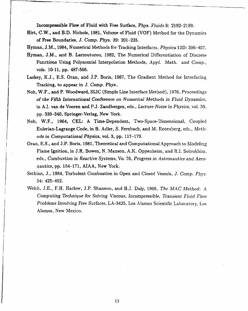
The final example of a captured interface is an ablation layer caused by the de-
position of laser energy on a solid target. One such calculation is shown in Figure 3,
taken from the work of Emery et al. (1982). The interface is the receding surface of
the solid target, on the left of the two calculations shown. As energy from the laser
is deposited on the surface of the target, a high-pressure plasma layer is formed. The
surface of the target is unstable to the Rayleigh-Taylor instability as a result of this
low-density, high-pressure layer. We generally think of this instability in terms of a
heavy fluid sitting on top of a light fluid in the presence of gravity. These calculations
were done with a two-dimensional Flux-Corrected Transport program similar to the
program that calculated the two-dimensional detonation just described. The difference
here is that there are now algorithms included for strong electron thermal conduc-
tion and inverse bremsstrahlung. The two panels show the nonlinear evolution of two
different wavelength perturbations at the interface.
MOVING-GRID METHODS
Moving-grid methods define the grid so that the interface is always located on cell
boundaries. Maintaining a cell boundary between different fluids controls numerical
smearing that can occur at the interface as the fluid is transported. The interface is
3

then a well defined continuous curve because it coincides with cell boundaries. There
are several approaches to actually implementing this idea. One is to maintain a grid
of distorted quadrilaterals (Hyman and Larrouturou, 1982). Another approach is to
use generalized orthogonal grids that fit the form of the interface. And yet another is
to use a Lagrangian r.epresentation with triangular cells (Fritts and Boris, 1979). We
might also try a combination methods that use a limited Lagrangian grid to represent
the interface as it moves through a rectangular Euleriari grid on which the overall fluid
problem is solved (Noh, 1964).
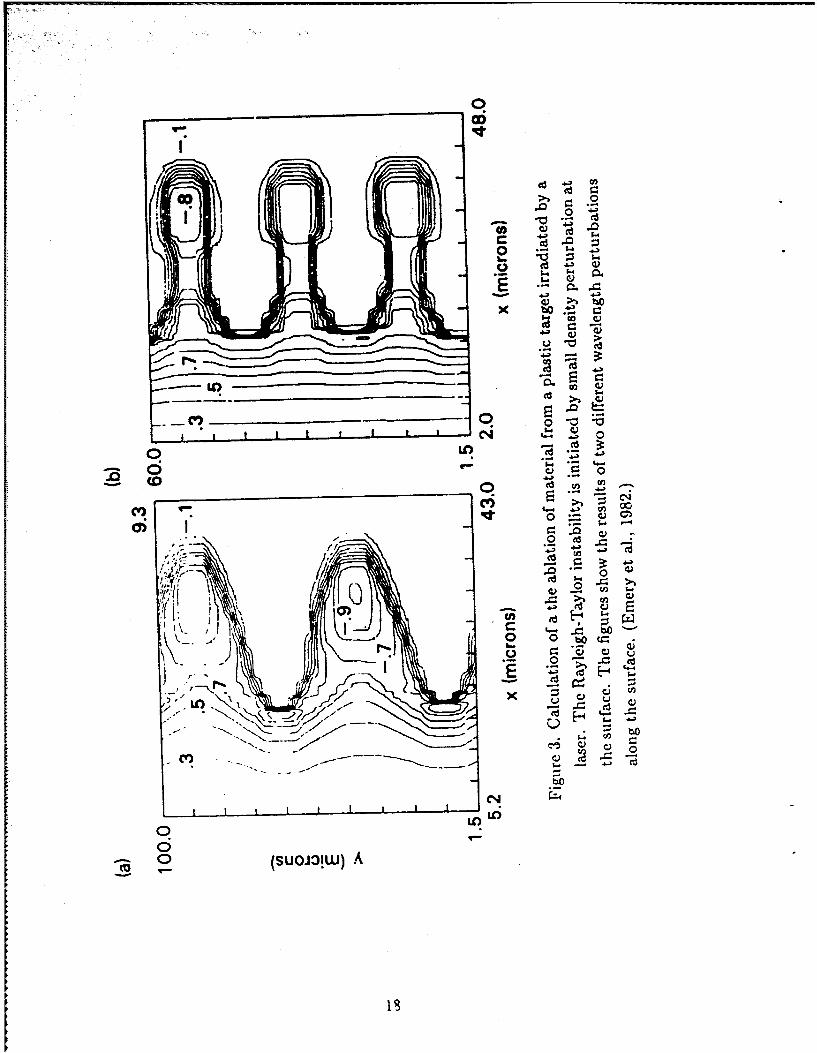
All of these approaches have advantages and disadvantages. The common advan-
tages are obvious: a potentially good representation of the interface. Using a quadrilat-
eral moving grid can cause problems, however, when there are motions in the flow that
severely distort the grid, as shown in Figure 4. One remedy requires defining a new grid
and interpolating the physical variable onto that grid. This interpolation introduces
iw"erical diffusion into the calculation. Some of the triangular grid approaches do
not have this problem, but instead have significant bookkeeping problems and h(;fty
computer storage requirements.
A combination of both an Eulerian grid and a superimposed Lagrangian grid i:;ries
to have the versatility of representing the interface on an adaptable grid and still keep
the convenient features of a rectangular grid for the fluid dynamics. In the CEL program
(Noh, 1964), a series of straight-line segments represents tL2 interface. For example, anisolated pocket of fluid would be bounded by an irregular polygon. The calculation for
one timestep proceeds in several steps. First, the Lagrangian grids defining interfaces
are advected through the Eulerian domain. Then, the calculations for the various fluids
are done on the Eulerian grid using the newly calculated Lagrangian positions of the
interface. Finally the velocity and pressure fields from the Eulerian calculation are
used to calculate the Lagrangian positions at the start of the next timestep. An initial
CEL gridding for a sample problem with a number of interfaces is shown in Figure 5.
Although methods such as CEL isolate the various fluids from each other, the problem
of distorting Lagrangian grids is still present. In addition, this method requires storing
information for both the Eulerian and Lagrangian grids, as well as rather expensivelogic and computation to interpolate back and forth between the two grids.
4
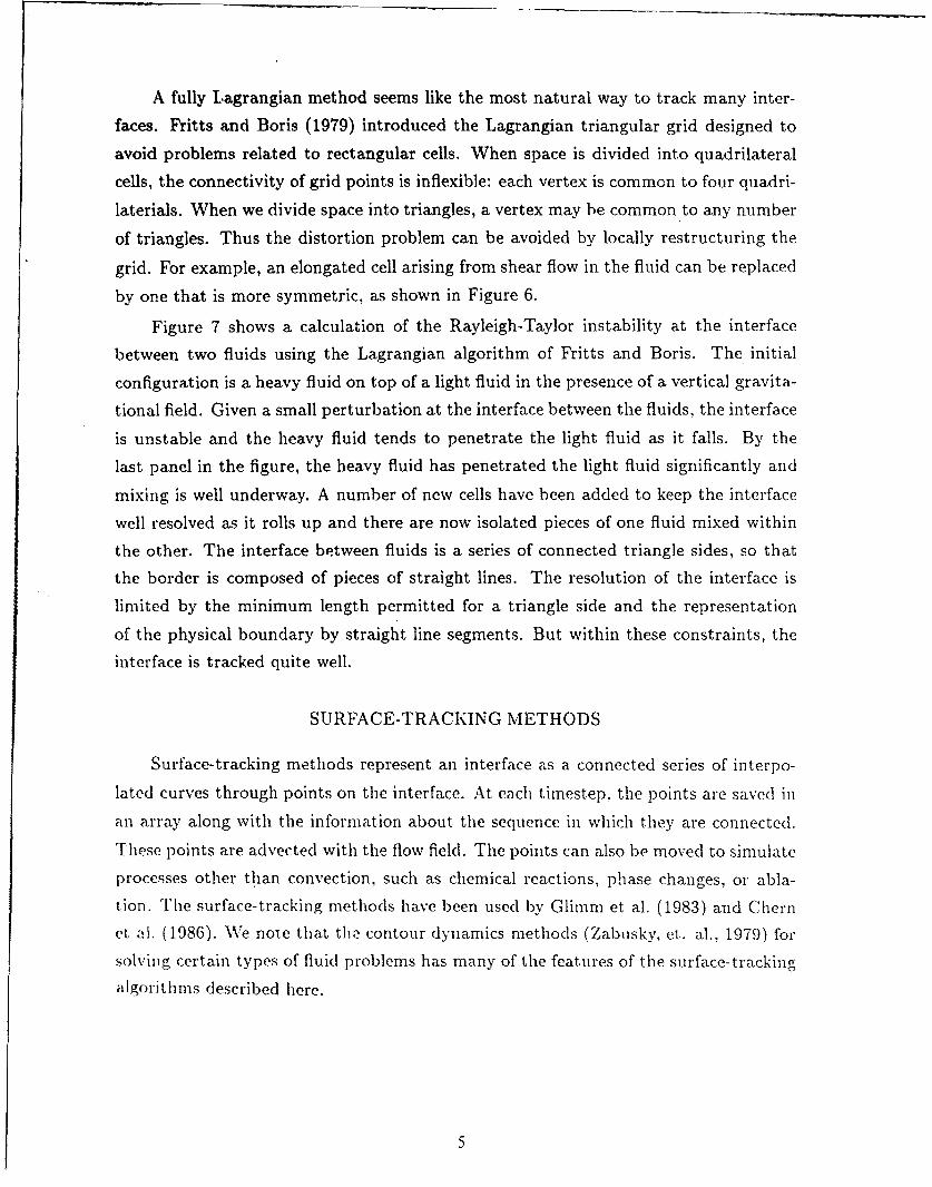
A fully Lagrangian method seems like the most natural way to track many inter-
faces. Fritts and Boris (1979) introduced the Lagrangian triangular grid designed to
avoid problems related to rectangular cells. When space is divided into quadrilateral
cells, the connectivity of grid points is inflexible: each vertex is common to four quadri-
laterials. When we divide space into triangles, a vertex may be common to any number
of triangles. Thus the distortion problem can be avoided by locally restructuring the
grid. For example, an elongated cell arising from shear flow in the fluid can be replaced
by one that is more symmetric, as shown in Figure 6.
Figure 7 shows a calculation of the Rayleigh-Taylor instability at the interface
between two fluids using the Lagrangian algorithm of Fritts and Boris. The initial
configuration is a heavy fluid on top of a light fluid in the presence of a vertical gravita-
tional field. Given a small perturbation at the interface between the fluids, the interface
is unstable and the heavy fluid tends to penetrate the light fluid as it falls. By the
last panel in the figure, the heavy fluid has penetrated the light fluid significantly and
mixing is well underway. A number of new cells have been added to keep the interface
well resolved as it rolls up and there are now isolated pieces of one fluid mixed within
the other. The interface between fluids is a series of connected triangle sides, so that
the border is composed of pieces of straight lines. The resolution of the interface is
limited by the minimum length permitted for a triangle side and the representation
of the physical boundary by straight line segments. But within these constraints, the
interface is tracked quite well.
SURFACE-TRACKING METHODS
Surface-tracking methods represent an interface as a connected series of interpo-
lated curves through points on the interface. At each timestep. the points are saved in
an array along with the information about the sequence in which they are connected.
These points are advected with the flow field. The points can also be moved to simulate
processes other than convection, such as chemical reactions, phase changes, or abla-tion. The surface-tracking methods have been used by Glimm et al. (1983) and Chern
et al. (1986). We note that the contour dynamics methods (Zabuskv. et. al., 1979) for
solving certain types of fluid problems has many of the features of the surface-trackingalgorithms described here.
5
In the simplest forms of surface-tracking methods for two dimensions, the points are
saved as a sequence of heights above a given reference line, as shown in Figure 8a. Two
curves are shown bounding the top and the bottom of a region of fluid. This approach
fails if the interpolated curve is multivalued or does not extend all the way across
the region. However, this problem may be avoided if the points follow a parametric
representation, such as that shown in Figure 8b. The parametric formulation is more
complex, but it can represent fine detail in th-? interface if enough points are used. An
interesting feature of these methods is that they can resolve features of the interface that
are smaller than the cell spacing of the macroscopic Eulerian grid on which the curves
are overlaid. There is naturally a price paid for storing this additional information.
The timestep for the entire calculation can be limited by the amount of movement the
interface can undergo during each timestep.
There are still two major problems. First, it is very difficult to handle merging
interfaces or joining a part of an interface to itself. This requires re-ordering the inter-
face points, which could require significant computational bookkeeping, and possibly
tracking additional interfaces. Second, for a giver. problem, the points can accumulate
in one segment of the interface leaving other segments without enough resolution. For
the most accuracy, it is best to limit the largest distance between neighboring points
to be something less than the minimum size of the local computation grid (Hirt and
Nichols, 1981). Interface areas typically increase continually in complex flows. Thus it
is necessary to add points along the interface automatically. Conversely, points should
be deleted where there are too many. When points must be added or deleted, the best
way to interpolate new points and the best way to represent and manipulate contours
with changing lengths are major computatonal issues.
Development of surface-tracking methods continues, but the problems of changing
topology from simply connected to multiply connected regions, merging fronts. disap-
pearance of weakened fronts, and the appearance of new fronts have yet to be solved.
The methods have generally been used in one- and two-dimensional calculations for
interfaces that do not interact. The complexity in specifying an interface and treat-
ing three-dimensional interactions may lnimt applications of surface tracking in three
dimensions.
6

VOLUME-TRACKING METHODS
Unlike the surface-tracking methods that store a representation of the interface,
volume-tracking methods reconstruct the interface whenever it is needed. The recon-
struction is done cell by cell and is based on the presence of a marker quantity within
the cell. Whereas the surface-tracking methods represent the interface by a continu-
ous curve, the interface generated by volume tracking consists of a set of disconnected
segments from the cells containing parts of the interface.
The earliest volume-tracking methods used marker particles so that the density
of particles in each cell indicates the density of the material. This method was first
proposed by Harlow (1955) and was called the Particle-in-Cell or PIC method. In the
Marker-and-Cell or MAC method (Harlow and Welch, 1965; Welch et al., 1966), the
particles are tracers, marker particles with no mass.
As in example, we consider some of the features of the PIC method implemented by
Amsden (1966). PIC uses an Eulerian grid in which velocity, internal energy, and total
cell mass are defined at cell centers. In addition, the different fluids are represented by
Lagrangian mass points, the marker particles, that move through the Eulerian grid. The
marker particles each have a constant mass, a specific internal energy, and a recorded
location in the Eulerian grid, and are moved with a local velocity. The particle mass,
momentum, and specific internal energy are transported from one cell to its neighbor
when the marker particle crosses the cell boundary. Cells containing marker particles
of both fluids contain the interface. Since the interface can be reconstructed locally at
any time, the problems associated with interacting interfaces and large fluid distortions
are eliminated. The method generalizes to any number of fluids.
Unlike the surface-tracking methods, marker-particle methods cannot resolve de-
tails of the interface which are smaller than the mesh size. However, the methods are
still expensive with respect to their requirements in computer time and memory. As
with the surface-tracking methods, particles may accumulate in portions of the grid,
thus leaving other portions not well enough resolved. Since mass, momentum, and
energy are associated with each particle in the PIC method. addition and deletion of
7

particles is not that straightforward. Unacceptable statistical fluctuations arise when
there are not enough marker particles and when the local variation of the attributes of
the marker particles is too large.
Many of the volume-tracking methods use the fraction of a cell volume occupied
by one of the materials as the marker for reconstructing the interface. If this fraction
is zero for a given cell, the material does not occupy the cell and there is no interface
in that cell. Conversely, if the fraction is one, the cell is completely occupied by the
material and again there is no interface present. An interface is constructed only if the
fractional marker volume is between zero and one.
The Simple Line Interface Calculation (SLIC) algorithms were first proposed by
Noh and Woodward (1976). Each grid cell is partitioned by a horizontal or vertical line
such that the volume of the partitioned part o' the cell equals the fractional marker
volume. The orientation of the line is chosen so that as to keep similar types of fluid in
neighboring cells adjacent. Thus a preference is given for lines through cells that are
normal to the direction of flow. Given a cell with an interface separating two fluids,
if the contents of this cell flows into an adjacent cell containing only one of the fluids,
then an interface orientation normal to the flow direction causes all of the common fluid
to move across the cell boundary before the second fluid enters the initially single-fluid
adjacent cell. This minimizes numerical diffusion between cells. The method assumes
timestep splitting is used in multidimensional problems, so that extensions to two or
three dimensions are straightforward. For the two-dimensional case, the interface is
constructed cell by cell before advection in the x-integration. After the x-integration,
the interface is reconstructed and the y-integration is done. Line segments normal to
the direction of flow usually result in different representations of the interface for the
and y-sweeps. To avoid such a directional bias, the order of x- and y-integrations
is changed every timestep. Samples of SLIC interface approximations are shown in
Figures 9 and 10.
Chorin (1980) improved the resolution of the original SLIC algorithm by adding a
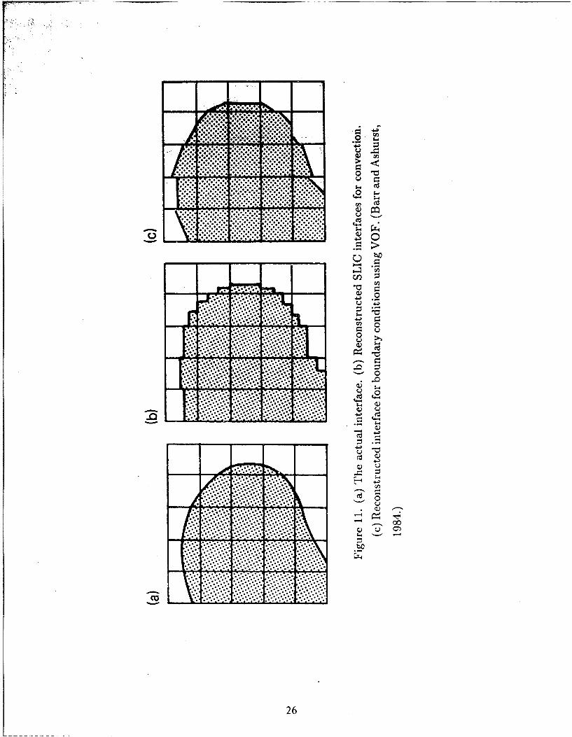
corner interface to the straight horizontal and vertical lines used bv Nob and Woodward,
but still using the same fractional cell volume as the variable for locating the interface.
:%n example of this SLIC interface is shown in Figure lib. Chorin used the vortex
8

dynamics method to calculate the vorticity field. The vorticity gives the velocity field
and these velocities are used to advect the interface. Advection is done in the sam
time-split manner as for the .r•iginal SLIC algorithm.To simulate the evolution of the interface. in particular, flame propagation, ChorT1
uses an idea based on Huygens' principle. Given a number of different directions, the
interface is propagated at a known speed in each of the directions separately and
the effect on the volume fractions for each propagation direction is stored. The final
interface position is the position that assigns the largest increase in the burned volume
to each cell. Chorin chose eight directions at angles aI = (I - 1),r/4, I = 1,.. ., 8.
Each pr, ipagation was carried out using the same timestep-splitting przcess as for the
advection. In the straightforward application of this idea, it is possible for interfaces
which initially start out as circles to evolve into octagons. Such problems are due to
preferential propagation in the eight directions. They may be avoided in several ways,
for example, by using random starting angles. This interface construction, advection.
and propagation sequence appears in combustion studies by Ghofniem et al. (1981,
1986) and Sethian (1984).
The VOF method of Hirt and Nichols (1981) also represents the interface within
a cell by a straight line, but the line may have any slope. A numerical estimate of
the x-direction and y-direction derivatives of the volume of fluid occupying a cell are
obtained for a given cell. If the magnitude of the x-direction derivative is smaller
than the magnitude of the y-direction derivative, then the interface is more nearly
horizontal and its slope is the value of the x-direction derivative. A more vertical
interface has a slope equal to the value of the y-direction derivative. If the x-directionderivative represcntb the slope of the interface, then the sign of the y-direction derivative
determines whether the fluid is above (positive) or below (negative) the interface. For
a more vertical line, the sign of the x-direction derivative identifies the location of the
marker fluid to the right (positive) or the left (negative) of the interface. Thus, giveu
the slope of the interface and the side of the interface on which the fluid is located,
the position of the interface within the cell is set. This process is done for every cell
with an occupied volume between zero and one. Hirt and Nichols use values of the
fractional volume of fluid averaged over several cells to calculate the derivatives. Other
9
implementations of VOF use a simple central difference (Barr and Ashurst, 1984).
The VOF method depends on the ability to advect the volume fraction through
the grid accurately without smearing from numerical diffusion. Hirt and Nichols have
described a "donor-acceptor" method to insure that only the appropriate constituent
fluid moves to or from a cell containing an interface. This helps to avoid cell averaging
that results in numerical diffusion.
To analyze combustion problems, Barr and Ashurst (1984) use both VOF and the
Chorin version of SLIC in a method called SLIC-VOF. The SLIC algorithm is used to
defime and advect interfaces and VOF is used to define the normal direction and to give
a smoother interface for the flame propagation phase. Figure 11 sh.,ws how SLIC and
VOF approximate the same curved interface. For a two-dimensional flame propagation
problem, SLIC-VOF performs the x integration of the SLIC interface, the y integra-
tion of the SLIC interface, the x-direction flame propagation of the VOF interface, and
then the y-direction flame propagation of the VOF interface. The interfaces are re-constructed following each advection or propagation calculation. At each timestep, the
order of the x- and y-sweeps are interchanged, but convection always precedes burning.
As in the Chorin implementation, flow velocities are calculated from a vorticity field.
The flame propagation speed in the x- and y-directions is the respective vector compo-
nent of a velocity vector normal to the interface defined by VOF with the magnitude
of the specified flame speed.
Barr and Ashurst (1984) give a detailed discussion of the problems with SLIC at-
gorithms. In brief, curved surfaces may be flattened or even indented. This distortion
depends oil the Courant number of the flow and the interface geometry. In some cases
this distortion appears as the interface first moves across a cell and does not increase
.thereafter. In other cases the distortion continues to grow. Including a model for prop-
agating chemical reactions apparently decreases this distortion since the propagation
step smooths short-wvavelength wrinkles.
THE GRADIENT METttOD
The gradient nmethod (Laskey et al.. 19S7) does not attempt to define the exact
location of tihe interface within a cell. but it represents the interface as a relatively
10

continuous gradient over several cells. By keeping the resolution of the interface at the
limit of that of the numerical convection algorithm, the amount of surplus computer
storage requirements and the cost of interface tracking can be reduced. Laskey has
applied this method to flame fronts, although it may also be useful for :. Ier types of
interfaces. We briefly describe some of the elements of the flame front tracking problem
because of its importance in reactive flows.
A system of gases react to form a product whose number density is nP. We solve
an equation of the formn+ np"= w(11 -2.1)
where nP is the number density of product and the right hand side is the production
term. The left hand side can be solved by any method for solving continuity equations.
The production term is added to the solution of the convection by timestep-splitting
methods. Conservation among the reactants and the product determines the amount
of energy released in each cell.
In this method, the reaction fronts are identified by the region in which there is
a large gradient, that is, where VnP is large. The integral of the gradient from the
front to the back of the extended interface is known. This is used to define a local
energy release rate and tends to guarantee the correct overall energy release along
the convoluted front. The gradient is assumed to be the result of the presence of the
reaction front, and thus, the amount of new product formed is
Anp = IVnp1l , (11 -2.2)
where Anp is the change in nP and I is the distance the front moves normal to itself
locally during the time interval of interest. The direction of the normal to the reaction
front is the same as the direction of the gradient. The speed of the front is the local
burning velocity. Therefore I is approximated by
I = VbAt,- (11--2.3)
where Vb is the local flame speed normal to the interface. The amount of product
formed per unit volume in the time interval At is
w =- Anp =.VbAtIln[. (11 -2.4)
11
The calculation requires determining jVnp,. Laskey et al. (1987) have found that
the one-sided difference approach for evaluating tLe gradient, although technically only
first-order accurate, gives better results than a second-order central difference. In
addition, there are several tests which must be made oyi the gradient to determine if
the numerical estimate of the gradient is a valid quantity. Finally, some modification
is required for the case of a nonuniform temperature field. The burning velocity vb
becomes a function of position and the number densities considered must be scaled to
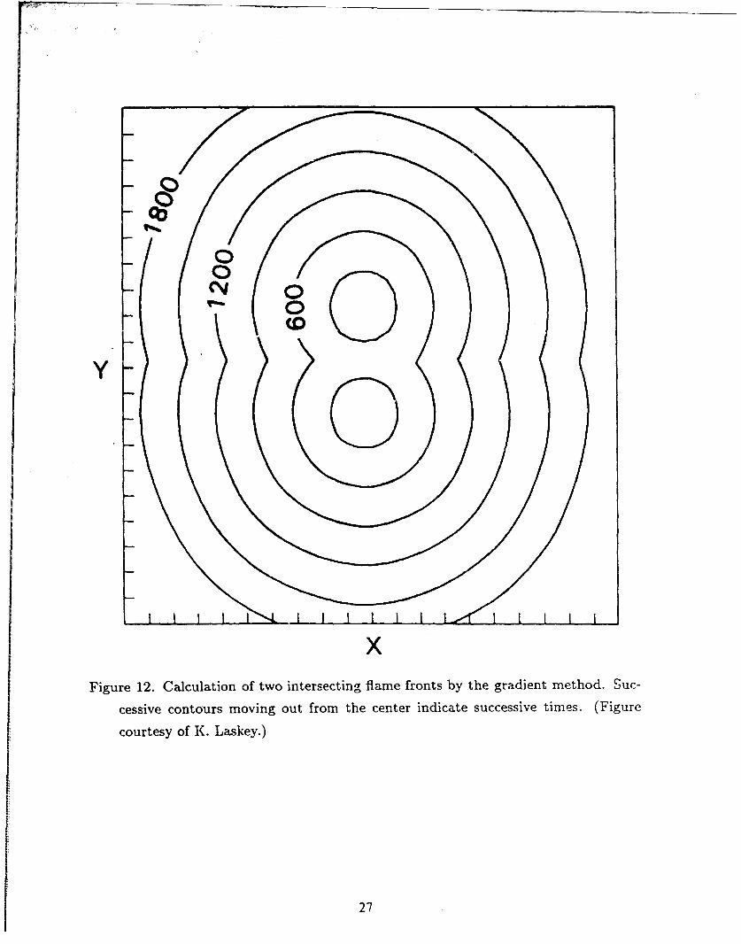
a reference temperature. An example of a gradient method calculation of two round
flame fronts that grow anc. merge is shown in Figlre 12.
There are several good features of the gradient meL.-d. It ensures that the right
amount of reaction takes place in the vicinity of the gradient, as defined by the macro-
scopic grid. Also, it treats the effects of merging interfaces with relatively little diffi-
culty. Adding other interface processes, and eventually ignoring weakened interfaces
results naturally from the formulation. Because no additional variables are needed,
computer memory requirements are modest. The algorithm as implemented is fully
vectorized. Finally, it is straightforward to extend the two-dimensional formulation to
three dimensions.
There are several drawbacks to the gradient method. As with the volume tracking
methods, the location of the reaction front is only approximately known. Thus, if it is
necessary to track the curvature at the surface on scales comparable or smaller than
the Eulerian grid spacing, another method should be used. An example of a problem
for which the gradient method is not suited is the dynamics of a droplet in which it is
important to know the curvature of a surface very accurately for calculating the effects
of surface tension. (see, for example, Fyfe et al., 1987).
Probably the most important limitation is that the gradient method assumes the
largest gradients appearing within the computational domain are located at the in-
terface and are the direct result of the existence of the interface. If large gradients
exist apart from the interface, then the gradient method may not be appropriate. An
analagous problem can plague any interface-tracking method which reconstructs the in-
terface using some quantity which should be indicative of the interface. If this quantity
is contaminated, spurious interfaces may result.
12
An important requirement of the gradient method is the gradients that the method
tries to represent remain quite large. This requires an advection algorithm which
minimizes numerical diffusion of the quantity used to define the interface. For this
purpose the present implementation of the gradient method is used in conjunction
with a high-order nonlinear monotone methods, such as Flux-Corrected Transport.
SUMMARY
A review has been presented of various approaches to modeling interfaces in nu-
merical simulations. Interface capturing methods attempt to resolve the details of the
structure of the interface and are most useful when the interface structure is crucial to
the calculation. However, numerically capturing an interface requires fine gridding on
the scale of the structure and very accurate values for input physical properties. If it is
not necessary to resolve the detailed structure of the interface, then the interface can
be treated as a discontinuity and interface tracking is useful.
There are several types of interface tracking methods. Surface-tracking methods
track discrete points on the interface while volume-tracking methods use a marker
quantity to reconstruct the interface when it is needed. Moving-grid methods alter
the computational grid so that the interface is always along cell boundaries. In all
these interface tracking methods, an exact location of the interface is defined prior to
calculating the interface effects. The gradient method differs from these in that theeffect of the interface is calculated without defining the interface location; the location
can be reconstructed for diagnostic purposes after the calculation is complete. Like the
volume-tracking methods, the calculation for the gradient method is based on a marker
quantity carried with the flow.
All of these methods are idiosyncratic. They work best under a specific set of
conditions, and are not totally general purpose. Therefore, the various strengths and
limitations of each of the interface tracking methods makes the choice of method de-
pendent on the problem at hand.
13
REFERENCES
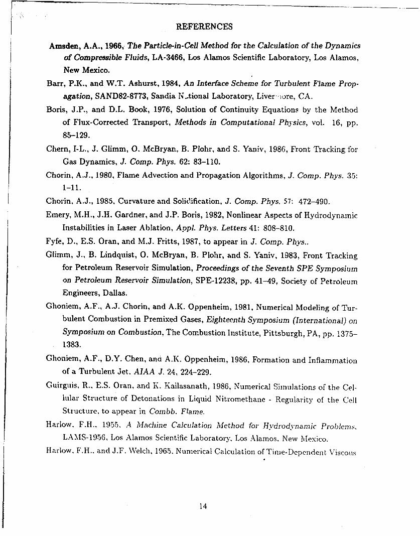
Amsden, A.A., 1966, The Particle-in-Cell Method for the Calculation of the Dynamicsof Compressible Fluids, LA-3466, Los Alamos Scientific Laboratory, Los Alamos,
New Mexico.
Barr, P.K., and W.T. Ashurst, 1984, An Interface Scheme for Turbulent Flame Prop-
agation, SAND82-8773, Sandia N.tional Laboratory, Liver iore, CA.
Boris, J.P., and D.L. Book, 1976, Solution of Continuity Equations by the Method
of Flux-Corrected Transport, Methods in Computational Physics, vol. 16, pp.
85-129.
Chern, I-L., J. Glimm, 0. McBryan, B. Plohr, and S. Yaniv, 1986, Front Tracking for
Gas Dynamics, J. Comp. Phys. 62: 83-110.
Chorin, A.J., 1980, Flame Advection and Propagation Algorithms, J. Comp. Phys. 35:
1-11.
Chorin, A.J., 1985, Curvature and Solidification, J. Comp. Phys. 57: 472-490.
Emery, M.H., J.H. Gardner, and J.P. Boris, 1982, Nonlinear Aspects of Hydrodynamic
Instabilities in Laser Ablation, Appl. Phys. Letters 41: 808-810.
Fyfe, D., E.S. Oran, and M.J. Fritts, 1987, to appear in J. Com p. Phys..
Glimm, J., B. Lindquist, 0. McBryan, B. Plohr, and S. Yaniv, 1983, Front Tracking
for Petroleum Reservoir Simulation, Proceedings of the Seventh SPE Symposium
on Petroleum Reservoir Simulation, SPE-12238, pp. 41-49, Society of Petroleum
Engineers, Dallas.
Ghoniem, A.F., A.J. Chorin, and A.K. Oppenheim, 1981, Numerical Modeling of Tur-bulent Combustion in Premixed Gases, Eighteenth Symposium (International) on
Symposium on Combustion, The Combustion Institute, Pittsburgh, PA, pp. 1375-
1383.
Choniem, A.F., D.Y. Chen, and A.K. Oppenheim, 1986, Formation and Inflammation
of a Turbulent Jet. AIAA J. 24, 224-229.
Guirguis, R., E.S. Oran, and K. Kailasanath, 1986, Numerical Simulations of the Cel-
lular Structure of Detonations in Liquid Nitromethane - Regularity of the Cell
Structure, to appear in Combb. Flame.
Harlow. F.H., 1955, A Machine Calculation Method for Hydrodynamic Problem•s.
LAMS-1956, Los Alamos Scientific Laboratory, Los Alamos. New Mexico.
Harlow, F.H.. and J.F. Welch, 1965, Numerical Calculation of Time-Dependent Viscous
14
Incompressible Flow of Fluid with Free Surface, Phys. Fluids 8: 2182-2189.
Hirt, C.W., and B.D. Nichols, 1981, Volume of Fluid (VOF) Method for the Dynamics
of Free Boundaries, J. Comp. Phys. 39: 201-225.
Hyman, J.M., 1984, Numerical Methods for Tracking Interfaces, Physica 12D: 396-407.
Hyman, J.M., and B. Larrouturou, 1982, The Numerical Differentiation of Discrete
Functions Using Polynomial Interpolation Methods, Appl. Math. and Comp.,
vols. 10-11, pp. 487-506.
Laskey, K.J., E.S. Oran, and J.P. Boris, 1987, The Gradient Method for Interfacing
Tracking, to appear in J. Comp. Phys..
Noh, W.F., and P. Woodward, SLIC (Simple Line Interface Method), 1976, Proceedings
of the Fifth International Conference on Numerical Methods in Fluid Dynamics,
in A.I. van de Vooren and P.J. Zandbergen, eds., Lecture Notes in Physics, vol. 59,
pp. 330-340, Springer-Verlag, New York.
Noh, W.F., 1964, CEL: A Time-Dependent, Two-Space-Dimensional, Coupled
Eulerian-Lagrange Code, in B. Adler, S. Fernbach, and M. Rotenberg, eds., Meth-
ods in Computational Physics, vol. 3, pp. 117-179.
Oran, E.S., and J.P. Boris, 1981, Theoretical and Computational Approach to Modeling
Flame Ignition, in J.R. Bowen, N. Manson, A.K. Oppenheim, and R.I. Soloukhim,
eds., Combustion in Reactive Systems, Vo. 76, Progress in Astronautics and Aero-
nautics, pp. 154-171, AIAA, New York.
Sethian, J., 1984, Turbulent Combustion in Open and Closed Vessels, J. Comp. Phys.
54: 425-452.
Welch, J.E., F.H. Harlow, J.P. Shannon, and B.J. Daly, 1966, The MAC Method: A
Computing Technique for Solving Viscous, Incompressible, Transient Fluid Flow
Problems Involving Free Surfaces, LA-3425, Los Alamos Scientific Laboratory, Los
Alamos, New Mexico.
15

1.019 - H2 -
H20 02
10 1 8
E 117 H>" • H20
zw 0 1 60 10 HO
w13 H On: 015-
z 10 02
01014--
H02
10 0 0.2 0.4 0.6 0.8 1.0
POSITION (cm)
Figure 1. Calculation of the chemical structure of a flame propagating in a mixture of
hydrogen and oxygen (Oran and Boris, 1981.)
16

(c
0~ ~ 0
00
LU-
0 3d
c2-.
I- oLL0
17 4
010 -
c~co
0 ~ 4.
C6 1
S.. S.
0) If.
1;'-, .)-~WD
.,'~ - .0 *bo
1' ~\ .
0.~ 0 0 bOCW CA
(dl (e)
W W
Figure 4. A Lagrangian calculation of a Rayleigh-Taylor instability with quadrilaterial
cells. The arrow indicate the location of the interface on each side ofr the figures.
A heavy fluid is on top of the light fluid, and the effects of gravity are included. A
small perturbation at the interface at the beginning of the calculation initiates the
instability. By (b), the calcuation cannot proceed because grid lines have crossed.
Regridding is then necessary. (Figure courtesy of M. Fritts.)
19

V
x
Figure 5. A possible initialization for a problem with multiple interfaces using the CEL
method. (Figure courtesy of W. Noh.)
20

4.7
blO
V 40 c'e
o -;:I
.- 0 a.-0
4J, 41
o d o
S0 P.
.- -1
Hn bI,a w~*
.r- *
1-4 bZ
0
21 1

5.00 x10⁻⁴ s 7.55 x10⁻² S
1.0 1.0
0.0 0.01.0.0 1.0 0.01.
1.01 x10 1 s 1.34 x1011.0 1.0
0.0 1.0 0.0.0 1.0
Figure 7. Sequence showing the evolution of a Rayleigh-Tyo intblt3 clucc
with a reconnecting Lagrangian grid of triangles. (Figure curtesy of Fi. Fitts.},
22

cd
4C
c) e
'4.
cd 0
cn >.
'C)
coo
32

-o.~0
0
-n -
24

) ________________________________________________
-� x
- 43
4300
�-1_________ _________ � -oo �43
0
�i2
C,)
2; x 43
4343
�0t4�4�- 0
43
s-I 43
__________ 43
Ci)
43 s-IC.)c�Q
C1)
-� x -�
_____ s-I
25
% :%
4-2
* * ~ .**.>
ho
*-4
bo
26
0
0
0X
YI
xFigure 12. Calculation of two intersecting flame fronts by the gradient method. Suc-
cessive contours moving out from the center indicate successive times. (Figure
courtesy of K. Laskey.)
27