Microsoft Word - Qin_RPTST1877-6116/10 2010 Bentham Open
Application of DRM-Trefftz and DRM-MFS to Transient Heat Conduction Analysis
Leilei Cao 1,2
, Qing-Hua Qin *,2
1 School of Mechatronics, Northwestern Polytechnical University, Xi’an 710072, P.R. China
2 Department of Engineering, Australian National University, Canberra, ACT 0200, Australia
Abstract: In this article we present two numerical models for solving transient heat conduction problems. One is based on
dual reciprocity method and Trefftz method (dubbed DRM-Trefftz), and the other is based on dual reciprocity method and
fundamental solution (dubbed DRM-MFS). A time stepping method is used in handling the time variable to convert the
problem into a set of inhomogeneous modified Helmholtz equations. The solution of the modified Helmholtz equation is
divided into two parts, i.e. the particular solution and the homogeneous solution. While the particular solution is solved by
DRM in which the source term is approximated by radial basis functions (RBF), the homogeneous solution is obtained by
using MFS or Trefftz method. Two types of bases functions, Trefftz solution and Fundamental solution are used to
approximate the homogeneous solution. The proposed two meshless methods require only discrete nodes constructed on
domain and boundary. Finally, the parameters that influence the performance of the proposed method are assessed
through several numerical examples. The results are presented for illustrating the accuracy and efficacy of the proposed
numerical models.
1. INTRODUCTION
During the past decades, lots of new advanced materials and technologies have been developed and used in aerospace technology and engineering, such as functionally graded materials [1] (FGM) and shaped memory alloy (SMAs), which are used as thermal barrier coating in high- temperature turbine engine (see patent [2, 3]) and telescopic wing system (see patent [4, 5]), respectively. Since the material like FGM and SMA are always working under tough temperature environment in aerospace, so it is necessary to know the thermal properties of these materials and thermal performance of the corresponding structures. Therefore, transient heat conduction analysis plays an important role in many fields of space technology and engineering.
On the other hand, various numerical models were developed for analyzing transient heat conduction problems [6-11] during the past years, such as Finite Element Method (FEM), Finite Difference Method (FDM) and Boundary Element Method (BEM). Among the above methods, FDM and FEM critically depend on the quality of mesh; however, generating a good quality of mesh for complicated geometry can be time-consuming. BEM involves only discretization of the boundaries which is an important advantage over FEM and FDM. However, the classical use of BEM for transient fields [12], based on discretization in time, usually results in domain integrals which may increase computing time and even cause some numerical problems and make BEM
*Address correspondence to this author at the Department of Engineering,
College of Engineering and Computer Science, The Australian National
University, Canberra, ACT 2601, Australia; Tel: +61 2 6125 8274; Fax: +61
2 6125 0506; E-mail: qinghua.qin@anu.edu.au
relatively inefficient compared to FEM and FDM. The Dual Reciprocity Method [13] (DRM) offers a solution method to avoid domain integration and hence became very popular recently. In particular, the dual reciprocity boundary element method (DRBEM), which transforms domain integrals to the boundary integrals by combining radial basis functions and conventional BEM, has wide applications in practical engineering. Applications of this approach to transient heat conduction problems can be found in [10, 14-16]. The multiple reciprocity boundary element method (MRBEM) has been emerging as a promising method for handling domain integrals [17]. However, DRBEM and MRBEM require more sophisticated mathematical procedures and the EEM itself involves further numerical integrations with a singular integral.
Alternatively, an attractive option is the meshless discretization approach which has received considerable attention by mathematicians and engineers in recent years. Meshless methods only use a number of nodes scattered within the problem domain and on the boundary. Among the existing meshless methods, the techniques most commonly used are the method of fundamental solutions (MFS) [18-21] and methods based on the radial basis functions (RBF) [22- 24]. The classical MFS is based on the approximation of the solution of a Boundary Value Problem (BVP) by a linear combination of fundamental solutions to the corresponding differential operator. The boundary conditions are then fitted by solving the linear system formed using a number of a collocation points. The singularities are avoided by the use of virtual boundaries outside the problem domain. The MFS is also known as the superposition method [25] and charge simulation method [26]. However, MFS has its limitation in that it can only solve homogeneous problems. The combination of MFS and RBF enables one to extend MFS to
42 Recent Patents on Space Technology, 2010, Volume 2 Qinghua Qin
non-homogeneous problems and various types of time- dependent problems [11, 27].
In contrast to the MFS which is based on the fundamental solution, the Trefftz method is formulated using the family of T-complete functions which are homogeneous solutions for the governing equation. The Trefftz method was initiated in 1926 [28]. Since then, it has been studied by many researchers (Cheung et al. [29, 30], Zielinski [31], Qin [32, 33], Kita [34]). Unlike in the method of fundamental solution which needs source points to be placed outside the domain in order to avoid singularity, T-complete functions are non-singularity inside and on the boundary of the given region.
Motivated by some recent substantial advances on DRM, Trefftz and MFS, we propose DRM-Trefftz and DRM-MFS models for analysing transient heat conduction problems in this paper. First, the time stepping method is used in handling the time variable of the heat conduction process and then the system is replaced by a set of inhomogeneous modified Helmholtz equations. The solution of the modified Helmholtz equation can be divided into two parts, i.e. the particular solution and the homogeneous solution. The particular solution is solved by DRM in which the source term is approximated by radial basis functions (RBF), while, both the Trefftz method and MFS are employed to construct the homogeneous solution. The paper is organized as follows. The DRM-Trefftz and DRM-MFS models are introduced in Section 2, followed by numerical validations in terms of some 2D transient heat conduction problems in Section 3, and finally, some concluding remarks are presented based on the reported results in Section 4.
2. NUMERICAL METHOD AND ALGORITHMS
2.1. Basic Formulations of Transient Heat Conduction
Consider a two-dimensional heat conduction equation
which models an unsteady temperature distribution in a solid
(domain ). This problem is governed by the differential
equation:
k 2u( X ,t)+Q( X ,t) = c u( X ,t) / t (1)
With the boundary conditions:
u (2)
• Newman/nature condition
q (3)
• convective condition
c (4)
0 X (5)
where u( X ,t) is the temperature function, k is the specified
thermal conductivity,
dimensional operator, is the mass density, c is the
specific heat and the overhead bar designates the imposed
quantities. q represents the boundary heat flux defined as
q = k u / n and n is the unit outward normal to the
boundary . Furthermore, u
h
e
is the heat transfer coefficient and u is the environmental
temperature. For a well-posed problem, we have
=
u q c .
For convenience, boundary conditions (2)-(4) are expressed in a general form as
B
3 X ,t( ) (6)
written respectively as
2.2. Time-Stepping Scheme
In the literature there are different approaches to handle time variable, two of which are: (1) Laplace transform; (2) finite differencing in time. Since numerical inversion of the Laplace transform is often ill-posed, here we apply the finite difference scheme to handle the time variable. For a typical time interval [t
n , t
n+1 ] [0,T], u(X, t), its derivative with
respect to time variable t and Q (X, t) are approximated as [35]:
u X ,t( ) = u n+1
X( ) + 1( )un X( )
u X ,t( ) t
X( )
X( ) + 1( )Qn X( )
(8)
where the superscripts n and n+1 refer to subsequent time
instances and = t n+1
t n is the time step size. ( 0 1 )
is a real parameter that determines if the method is explicit
( = 0 ), implicit ( = 1 ) or a linear combination of both
types [36]. The special choice of = 1/ 2 is known as the
Crank Nicolson scheme in the literature.
It is easily verified that the conditions which prevent
oscillations in the explicit case are exactly the same as the
commonly cited sufficient conditions which ensure that it is
stable. Furthermore, even though a Crank Nicolson approach
is unconditionally stable, it permits the development of
spurious oscillations unless the time step size is no more than
twice that required for an explicit method to be stable.
Although an implicit scheme is only first-order accurate in
time, it is proved that the Partial differential Equation (PDE)
can be solved accurately using the implicit scheme [37].
Hence, we use = 1 in our analysis.
Substituting Eq. (8) into Eqs. (1) and (6) and rearranging
it yields the following modified Helmholtz-type equation
Application of DRM-Trefftz and DRM-MFS Recent Patents on Space Technology, 2010, Volume 2 43
that has to be solved at each time step t n+1
for the unknown
n+1 X( ) (10)
Note that the right-hand side of Eq. (9) is well defined in
terms of the approximate solution u n
calculated on the
u X ,0( ) = u
0 , the initial condition of the transient problem.
For simplicity, the single step formula Eq. (9) can be written as
( 2 2 )u( X ) = f ( X ) (11)
where
= c
Qn ( X )
k (13)
Eq. (11) is a sequence of inhomogeneous modified Helmholtz equation, the solution of which is discussed in the next section.
2.3. Implementation of the Proposed Meshless Method
Due to linear property of Eq. (11), its solution can be
expressed as a summation of a particular solution u
p and a
homogeneous solution u
h , that is:
( 2 2 )u
but does not necessarily satisfy the boundary conditions (2)-
(4), and u
u h ( X ,t) = u ( X ,t) u
p ( X ,t) X
p ( X ,t) X
h ( X ,t) = h u h u
p ( X ,t)+ q
p ( X ,t) X
c
(17)
Similar to the treatment of Eq. (6), Eq. (17) can be written in a general form:
B
Solution
p can be obtained by DRM. To
do this, the right-hand side term of Eq. (15) is approximated
by RBF [38], yielding
i=1
N I
X (19)
where N
domain under consideration. Here,
i( )
i
Simultaneously, the particular solution u
p is similarly
( 2 2 )
p and
function f ( X ) in Eq. (15).
By enforcing Eq. (20) to satisfy Eq. (15) at all nodes, we
can obtain a set of simultaneous equations to uniquely
determine the unknown coefficients i
. In this procedure,
we need to evaluate the approximate particular solutions in
terms of the RBF . The standard approach is that is first
selected, and then the corresponding approximate particular
solutions are determined by solving Eq. (21) analytically.
For the Laplace operator, can be obtained by repeated
integration, but for the Helmholtz-type operator, this has
proven difficult [24, 39]. A significant result for Helmholtz-
type operator was given by Chen and Rashed where analytic
formulas were given for when as a Thin Plate Spline
(TPS) [40]:
0.5772156649015328 is Euler’s constant.
44 Recent Patents on Space Technology, 2010, Volume 2 Qinghua Qin
Another scheme for obtaining approximate particular
solutions is a reverse approach [36, 37]. Here, is first
chosen directly and Eq. (22) is used to evaluate . For
example, the particular solutions are directly chosen as
follows [22]:
(r) = 1+ r
r 3
9 ) (25)
It is difficult to prove mathematically under what conditions this approach is reliable, although it seems to work well so far for many problems [41-43]
An additional polynomial term p is required to assure
nonsingularity of the interpolation matrix if the RBF is
conditionally positive definite such as TPS [44, 45]. And
also, to achieve higher convergence rates for f ( X ) , the
higher order splines are considered [46]. For example,
= r
2 (26)
n is a polynomial of total degree n and let
{b
j }
n (
P
boundary conditions are given by
i
n (28)
Since the inhomogeneous term f ( X ) in Eq. (11) is a
known function depending on the temperature field u n , the
coefficients i
Eq. (28). Then the particular solution can be obtained from
Eq. (20).
h . Here
MFS, which are based on Trefftz solution and fundamental
solution, respectively. The details are follows in the next
section.
Introducing polar coordinates (r, ) with r = 0 at the
centroid of , it is known that the set
N ={I
equation, where I
kind with order n .
u h
where c
j are the coefficients to be determined and m is its
number of components. The terms N
j ( X ) = N (r) = N X X
j( )
operator ( 2 ) , and
on the physical boundary of the solution domain. As an
illustration, the internal function N
j in Eq. (30) can be given
in the form
u h
h in Eq. (30) and (32)
automatically satisfies the given differential equation (16),
all we need to do is to enforce u
h to satisfy the modified
boundary conditions (17) as u
p has already been calculated
separately. To do this, collocation points {X
j }
on the physical boundary to fit the boundary condition (18).
It leads to a system of linear algebraic equations in matrix
form:
[A]
If the number of components equals to the number of
collocation points on the physical boundary (m = N
S ) , this
case the number of components is smaller than the number
of collocation points (m = N
S ) , this results in over-
determined equations. The least square method can be used
to solve the over-determined equations. Once {c}is obtained,
u
h can be computed at any location in the domain using Eq.
(30).
2.3.3. MFS for Homogeneous Solution
In the implementation of MFS, the homogeneous solution is approximated in a standard collocation fashion
u h
(35)
Application of DRM-Trefftz and DRM-MFS Recent Patents on Space Technology, 2010, Volume 2 45
where j
u
j
of the modified Helmholtz operator ( 2 ) . Here the
source points {X
domain.
u
j
0 is the modified Bessel function of the second kind
with order zero.
satisfies the given differential equation (16), we need to
enforce u
h to satisfy the modified boundary conditions (18)
as we did in Trefftz method. But unlike the Trefftz method,
MFS needs source points placed outside the solution domain
to avoid singularity. In addition, the same number
collocation points on the physical boundary are chosen to fit
the boundary condition (18). As before, it leads to a system
of linear algebraic equations in matrix form:
[A]
location in the domain using Eq. (35).
Additionally, the generation of source points outside the domain is a curious problem, which affects the accuracy and stability. Generally, the accuracy of the approximation improves as the distance between the virtual and physical boundaries increase. At the same time, the MFS equations can become highly ill-conditioned at this circumstance [38]. At present, there is no uniform approach to generate these source points properly. In our work, a strategy is employed [18]:
Y
of the domain and is a dimensionless parameter which is
arbitrarily chosen as 1.2 for the outer boundary.
2.3.4. The Construction of the Solution System
Based on above operations, the complete solution u X( )
for the modified Helmholtz equation can be written as
u X( ) = i i X( )
i=1
N I
i=1
N I
+ j u
q X( ) = u( X )
q X( ) = u( X )
nj=1
N S
X (43)
For the DRM-MFS method. Above is the basic idea of the proposed methods, we will give some numerical examples in the following section.
3. NUMERICAL EXAMPLES
In order to demonstrate the efficiency and accuracy of the
proposed meshless method and the selected RBF and virtual
boundary, two benchmark numerical examples of transient
heat conduction problems are considered for which
corresponding exact solutions are known and can be used for
verification. The domain in these two examples is a 3 3
square. In the computation,
assumed. The third example is more complicated with non-
smooth boundary.
results, the average relative error on a variable f is
introduced as
i=1
N (44)
where N is the number of test points and ( f ) i is an
arbitrary field function, such as a temperature at point i.
Example 1: Consider a classic heat diffusion problem
which has been studied using the finite element method by
Bruch and Zyvoloski [7], BEM with time-dependent
fundamental solutions by Brebbia and Wroble [8], DRBEM
by Partridge [13] and Trefftz finite element method by
Jirousek and Qin [9]. The initial temperature of the whole
domain is 30 o
shock ( u = 0 all over the boundary), the geometry and
boundary conditions of the problem are shown in Fig. (1).
u(0, y,t) = u(x,0,t) = u(3, y,t) = u(x,3,t) = 0,
u
u(x, y,t) = A n
32 ]
where
46 Recent Patents on Space Technology, 2010, Volume 2 Qinghua Qin
A n = 4 30
nj 2
Fig. (1). Geometry of square domain and boundary conditions for
example 1.
In order to investigate the effect of the component
number m in Eq. (30), the number of components is chosen
as 10, 20, 30 and 40, respectively, and 40 collocation points
in the calculation. It can be seen from Fig. (2) that the results
gradually converge to the exact values as the number of
components (m) increases. This can be explained by that the
least square method can achieve better numerical accuracy in
solving the over-determined equations when the number of
unknowns is close to the number of equations. But, from Fig.
(2) we also observe that a larger m leads to a larger
condition number of matrix A, which is not beneficial to
some complex problem. So, the optimal value of m should
be found by numerical experimentation. The value of m is
taken to be the same as the number of collocation points on
the boundary in the following numerical simulation.
Table 1 presents the results obtained by DRM-Trefftz
and DRM-MFS and other solutions, obtained with the same
value of time step ( = 0.05 ). For the sake of comparison,
the same space discretizaion as in Ref. [13] is employed. It
should be mentioned that the difference between BEM1 and
BEM2 in Table 1 is as follows [8]: with BEM1, internal cells
were employed in order to account for the initial conditions
at the beginning of each time step, while for BEM2, the
solution process always restarted at the initial time and
domain discretization was avoided. It can be seen clearly
from Table 1 that the results obtained by proposed meshless
methods (DRM-Trefftz and DRM-MFS) agree well with the
exact solution and appear to be more accurate than the
results obtained from other methods.
Fig. (2). Effect of various component number to numerical
accuracy and condition number of matrix A.
The error in the meshless methods can be split into two
parts: one is due to approximating homogeneous solutions
and the other is due to approximating particular solutions.
One phenomenon that should be noticed is that the two
meshless methods we proposed converge to the same value.
Since the same RBF is used to approximate particular
solutions for both DRM-Trefftz and DRM-MFS, it indicates
that Trefftz bases and MFS make the same contribution to
the error of the homogeneous part. That means, using Trefftz
bases and fundamental solution to approximate
homogeneous solutions can achieve the same accuracy. So,
DRM plays a very important role in the convergent
behaviour of the meshless methods. In order to evaluate the
efficiency of DRM, we employ different RBF (standard
method and reverse method) in DRM for assessment.
Moreover, for standard approach, splines with different order
are considered. In Table 2, Si ( i = 1 4 ) denote the results
gained by using splines
additional polynomial term ( = 0.05 ). For comparing
purpose, PSi ( i = 1 4 ) denote the results gained by using
Eq. (27) with additional polynomial terms P
i .
The numerical results in Table 2 show that the use of
higher-order RBF interpolation functions does not improve
computing accuracy in transient problems. A previous work
[46] showed that more accurate results can be obtained by
using higher order polyharmonic splines for elliptic
boundary value problems, but from the above results we can
see limited improvement for time-dependent problems,
presumably because the dominant error was caused by the
Table 1. Comparison of Results at t = 1.2
Point x y DRM-
FEM [9] Exact
1 2.4 1.5 1.0263 1.0263 1.114 1.122 1.139 1.099 1.103 1.065
2 2.4 2.4 0.5985 0.5985 0.657 0.663 0.670 0.645 0.660 0.626
3 1.8 1.5 1.6868 1.6868 1.798 1.809 1.843 1.784 1.797 1.723
4 1.8 1.8 1.6022 1.6022 1.713 1.721 1.753 1.695 1.715 1.639
5 1.5 1.5 1.7760 1.7760 1.887 1.902 1.938 1.877 1.894 1.812
y
3
0.1491
0.1493
0.1495
0.1497
0.1499
m
Condition number
Application of DRM-Trefftz and DRM-MFS Recent Patents on Space Technology, 2010, Volume 2 47
time-stepping scheme. Moreover, the higher-order
polyharmonic splines result in worse conditioning of the
linear system associated with the homogeneous solution.
Therefore, care must be taken in using higher-order RBFs. It
can be seen from the results that when the order i is even
( i = 2,4 ), adding additional polynomial terms can increase
the accuracy, but when the order i is odd ( i = 1,3,5 ), the
results are opposite. The reverse method is more accurate
than the standard method except for i = 1 (S1, PS1).
Moreover, the reverse method can save a lot of computing
time without calculating modified Bessel functions which is
quite complex and really time consuming. Therefore, the
reverse method is employed in the following computation.
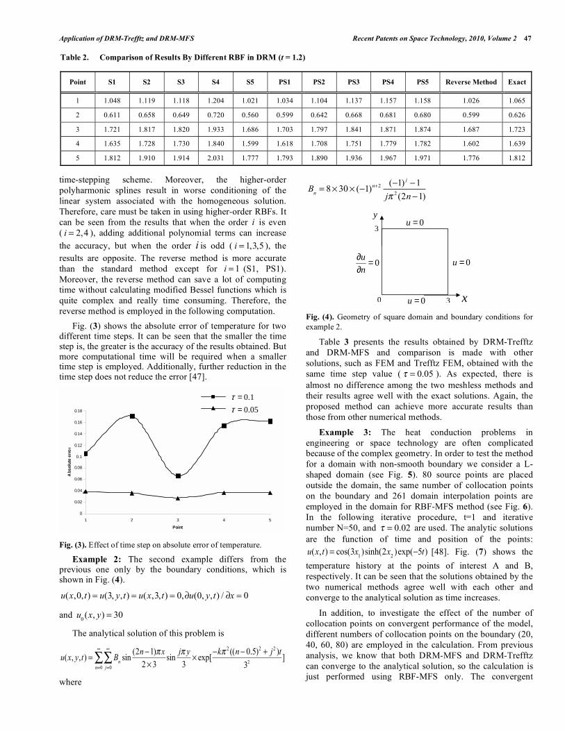
Fig. (3) shows the absolute error of temperature for two different time steps. It can be seen that the smaller the time step is, the greater is the accuracy of the results obtained. But more computational time will be required when a smaller time step is employed. Additionally, further reduction in the time step does not reduce the error [47].
Fig. (3). Effect of time step on absolute error of temperature.
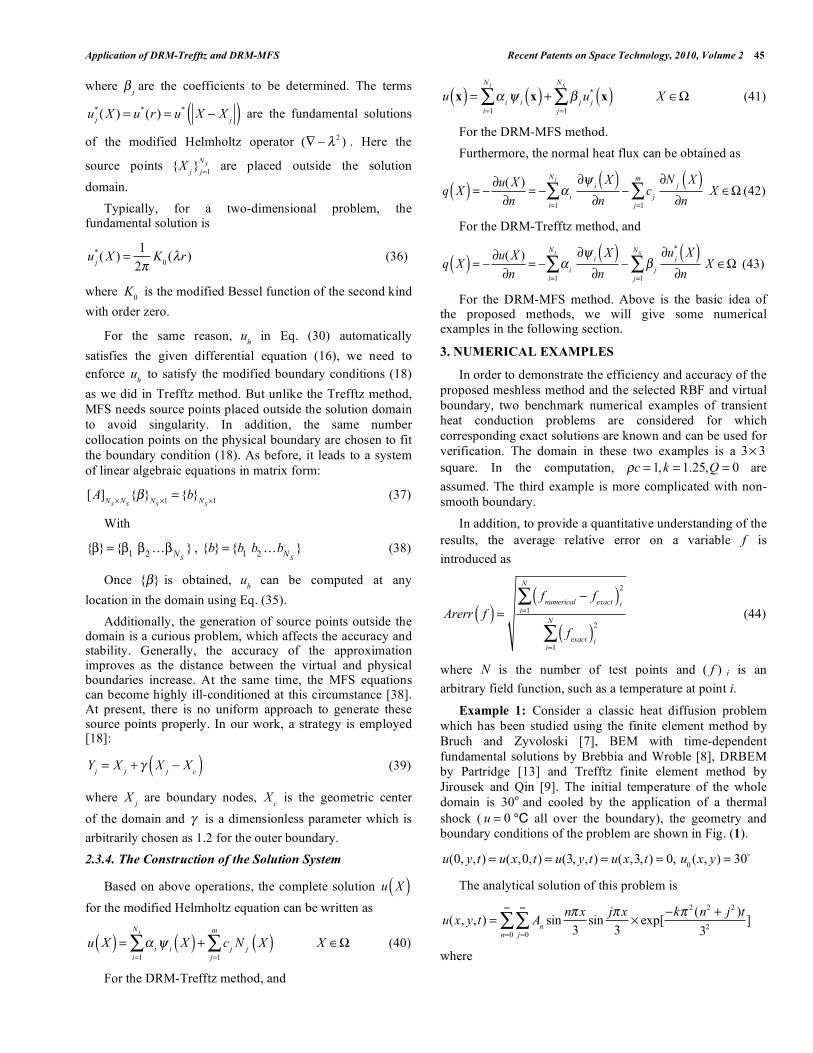
Example 2: The second example differs from the previous one only by the boundary conditions, which is shown in Fig. (4).
u(x,0,t) = u(3, y,t) = u(x,3,t) = 0, u(0, y,t) / x = 0
and u
u(x, y,t) = B n
32 ]
where
j 2 (2n 1)
Fig. (4). Geometry of square domain and boundary conditions for
example 2.
solutions, such as FEM and Trefftz FEM, obtained with the
same time step value ( = 0.05 ). As expected, there is
almost no difference among the two meshless methods and
their results agree well with the exact solutions. Again, the
proposed method can achieve more accurate results than
those from other numerical methods.
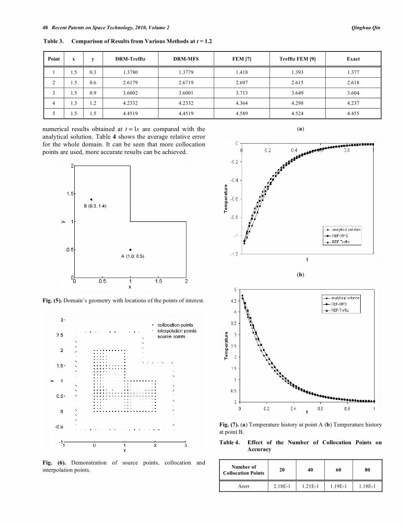
Example 3: The heat conduction problems in
engineering or space technology are often complicated
because of the complex geometry. In order to test the method
for a domain with non-smooth boundary we consider a L-
shaped domain (see Fig. 5). 80 source points are placed
outside the domain, the same number of collocation points
on the boundary and 261 domain interpolation points are
employed in the domain for RBF-MFS method (see Fig. 6).
In the following iterative procedure, t=1 and iterative
number N=50, and = 0.02 are used. The analytic solutions
are the function of time and position of the points:
u(x,t) = cos(3x
1 )sinh(2x
temperature history at the points of interest A and B,
respectively. It can be seen that the solutions obtained by the
two numerical methods agree well with each other and
converge to the analytical solution as time increases.
In addition, to investigate the effect of the number of
collocation points on convergent performance of the model,
different numbers of collocation points on the boundary (20,
40, 60, 80) are employed in the calculation. From previous
analysis, we know that both DRM-MFS and DRM-Trefftz
can converge to the analytical solution, so the calculation is
just performed using RBF-MFS only. The convergent
Table 2. Comparison of Results By Different RBF in DRM (t = 1.2)
Point S1 S2 S3 S4 S5 PS1 PS2 PS3 PS4 PS5 Reverse Method Exact
1 1.048 1.119 1.118 1.204 1.021 1.034 1.104 1.137 1.157 1.158 1.026 1.065
2 0.611 0.658 0.649 0.720 0.560 0.599 0.642 0.668 0.681 0.680 0.599 0.626
3 1.721 1.817 1.820 1.933 1.686 1.703 1.797 1.841 1.871 1.874 1.687 1.723
4 1.635 1.728 1.730 1.840 1.599 1.618 1.708 1.751 1.779 1.782 1.602 1.639
5 1.812 1.910 1.914 2.031 1.777 1.793 1.890 1.936 1.967 1.971 1.776 1.812
0
0.02
0.04
0.06
0.08
0.1
0.12
0.14
0.16
0.18
Point
0u =
48 Recent Patents on Space Technology, 2010, Volume 2 Qinghua Qin
numerical results obtained at t = 1s are compared with the
analytical solution. Table 4 shows the average relative error
for the whole domain. It can be seen that more collocation
points are used, more accurate results can be achieved.
Fig. (5). Domain’s geometry with locations of the points of interest.
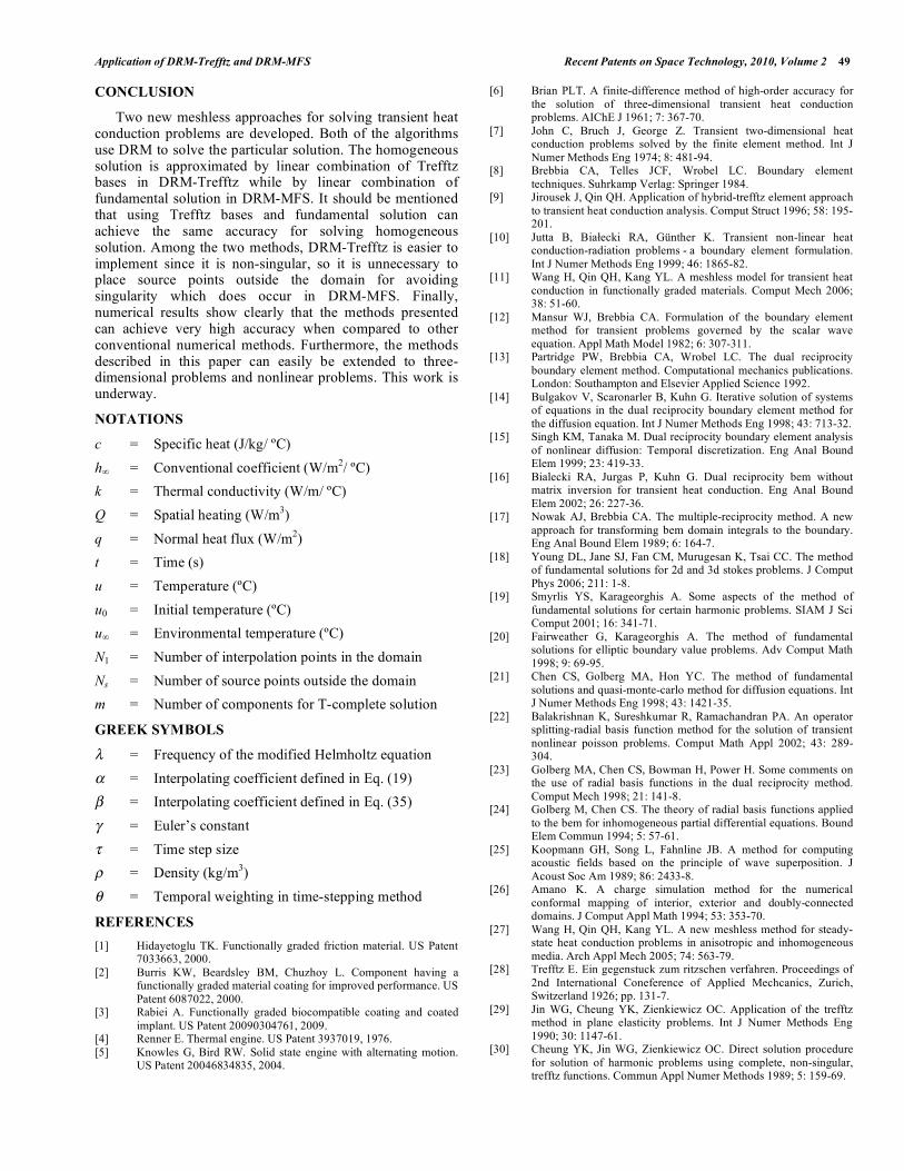
Fig. (6). Demonstration of source points, collocation and
interpolation points.
(a)
(b)
Fig. (7). (a) Temperature history at point A (b) Temperature history
at point B.
Table 4. Effect of the Number of Collocation Points on
Accuracy
Arerr 2.18E-1 1.21E-1 1.19E-1 1.18E-1
Table 3. Comparison of Results from Various Methods at t = 1.2
Point x y DRM-Trefftz DRM-MFS FEM [7] Trefftz FEM [9] Exact
1 1.5 0.3 1.3780 1.3779 1.418 1.393 1.377
2 1.5 0.6 2.6179 2.6719 2.697 2.615 2.618
3 1.5 0.9 3.6002 3.6001 3.713 3.649 3.604
4 1.5 1.2 4.2332 4.2332 4.364 4.298 4.237
5 1.5 1.5 4.4519 4.4519 4.589 4.524 4.455
Application of DRM-Trefftz and DRM-MFS Recent Patents on Space Technology, 2010, Volume 2 49
CONCLUSION
Two new meshless approaches for solving transient heat conduction problems are developed. Both of the algorithms use DRM to solve the particular solution. The homogeneous solution is approximated by linear combination of Trefftz bases in DRM-Trefftz while by linear combination of fundamental solution in DRM-MFS. It should be mentioned that using Trefftz bases and fundamental solution can achieve the same accuracy for solving homogeneous solution. Among the two methods, DRM-Trefftz is easier to implement since it is non-singular, so it is unnecessary to place source points outside the domain for avoiding singularity which does occur in DRM-MFS. Finally, numerical results show clearly that the methods presented can achieve very high accuracy when compared to other conventional numerical methods. Furthermore, the methods described in this paper can easily be extended to three- dimensional problems and nonlinear problems. This work is underway.
NOTATIONS
h = Conventional coefficient (W/m 2 / ºC)
k = Thermal conductivity (W/m/ ºC)
Q = Spatial heating (W/m 3 )
q = Normal heat flux (W/m 2 )
t = Time (s)
u = Temperature (ºC)
m = Number of components for T-complete solution
GREEK SYMBOLS
= Euler’s constant
= Time step size
= Density (kg/m 3 )
REFERENCES
[1] Hidayetoglu TK. Functionally graded friction material. US Patent 7033663, 2000.
[2] Burris KW, Beardsley BM, Chuzhoy L. Component having a functionally graded material coating for improved performance. US
Patent 6087022, 2000. [3] Rabiei A. Functionally graded biocompatible coating and coated
implant. US Patent 20090304761, 2009. [4] Renner E. Thermal engine. US Patent 3937019, 1976.
[5] Knowles G, Bird RW. Solid state engine with alternating motion. US Patent 20046834835, 2004.
[6] Brian PLT. A finite-difference method of high-order accuracy for
the solution of three-dimensional transient heat conduction problems. AIChE J 1961; 7: 367-70.
[7] John C, Bruch J, George Z. Transient two-dimensional heat conduction problems solved by the finite element method. Int J
Numer Methods Eng 1974; 8: 481-94. [8] Brebbia CA, Telles JCF, Wrobel LC. Boundary element
techniques. Suhrkamp Verlag: Springer 1984. [9] Jirousek J, Qin QH. Application of hybrid-trefftz element approach
to transient heat conduction analysis. Comput Struct 1996; 58: 195- 201.
[10] Jutta B, Bia ecki RA, Günther K. Transient non-linear heat conduction-radiation problems - a boundary element formulation.
Int J Numer Methods Eng 1999; 46: 1865-82. [11] Wang H, Qin QH, Kang YL. A meshless model for transient heat
conduction in functionally graded materials. Comput Mech 2006; 38: 51-60.
[12] Mansur WJ, Brebbia CA. Formulation of the boundary element method for transient problems governed by the scalar wave
equation. Appl Math Model 1982; 6: 307-311. [13] Partridge PW, Brebbia CA, Wrobel LC. The dual reciprocity
boundary element method. Computational mechanics publications. London: Southampton and Elsevier Applied Science 1992.
[14] Bulgakov V, Scaronarler B, Kuhn G. Iterative solution of systems of equations in the dual reciprocity boundary element method for
the diffusion equation. Int J Numer Methods Eng 1998; 43: 713-32. [15] Singh KM, Tanaka M. Dual reciprocity boundary element analysis
of nonlinear diffusion: Temporal discretization. Eng Anal Bound Elem 1999; 23: 419-33.
[16] Bialecki RA, Jurgas P, Kuhn G. Dual reciprocity bem without matrix inversion for transient heat conduction. Eng Anal Bound
Elem 2002; 26: 227-36. [17] Nowak AJ, Brebbia CA. The multiple-reciprocity method. A new
approach for transforming bem domain integrals to the boundary. Eng Anal Bound Elem 1989; 6: 164-7.
[18] Young DL, Jane SJ, Fan CM, Murugesan K, Tsai CC. The method of fundamental solutions for 2d and 3d stokes problems. J Comput
Phys 2006; 211: 1-8. [19] Smyrlis YS, Karageorghis A. Some aspects of the method of
fundamental solutions for certain harmonic problems. SIAM J Sci Comput 2001; 16: 341-71.
[20] Fairweather G, Karageorghis A. The method of fundamental solutions for elliptic boundary value problems. Adv Comput Math
1998; 9: 69-95. [21] Chen CS, Golberg MA, Hon YC. The method of fundamental
solutions and quasi-monte-carlo method for diffusion equations. Int J Numer Methods Eng 1998; 43: 1421-35.
[22] Balakrishnan K, Sureshkumar R, Ramachandran PA. An operator splitting-radial basis function method for the solution of transient
nonlinear poisson problems. Comput Math Appl 2002; 43: 289- 304.
[23] Golberg MA, Chen CS, Bowman H, Power H. Some comments on the use of radial basis functions in the dual reciprocity method.
Comput Mech 1998; 21: 141-8. [24] Golberg M, Chen CS. The theory of radial basis functions applied
to the bem for inhomogeneous partial differential equations. Bound Elem Commun 1994; 5: 57-61.
[25] Koopmann GH, Song L, Fahnline JB. A method for computing acoustic fields based on the principle of wave superposition. J
Acoust Soc Am 1989; 86: 2433-8. [26] Amano K. A charge simulation method for the numerical
conformal mapping of interior, exterior and doubly-connected domains. J Comput Appl Math 1994; 53: 353-70.
[27] Wang H, Qin QH, Kang YL. A new meshless method for steady- state heat conduction problems in anisotropic and inhomogeneous
media. Arch Appl Mech 2005; 74: 563-79. [28] Trefftz E. Ein gegenstuck zum ritzschen verfahren. Proceedings of
2nd International Coneference of Applied Mechcanics, Zurich, Switzerland 1926; pp. 131-7.
[29] Jin WG, Cheung YK, Zienkiewicz OC. Application of the trefftz method in plane elasticity problems. Int J Numer Methods Eng
1990; 30: 1147-61. [30] Cheung YK, Jin WG, Zienkiewicz OC. Direct solution procedure
for solution of harmonic problems using complete, non-singular, trefftz functions. Commun Appl Numer Methods 1989; 5: 159-69.
50 Recent Patents on Space Technology, 2010, Volume 2 Qinghua Qin
[31] Zielinski AP. On trial functions applied in the generalized trefftz
method. Adv Eng Softw 1995; 24: 147-55. [32] Qin QH. Trefftz finite element method and its applications. Appl
Mech Rev 2005; 58: 316-37. [33] Qin QH. Trefftz finite and boundary element method. Southamp-
ton: WIT Press 2000. [34] Kita E, Ikeda Y, Kamiya N. Trefftz solution for boundary value
problem of three-dimensional poisson equation. Eng Anal Bound Elem 2005; 29: 383-90.
[35] Chapko R, Kress R. Rothe's method for the heat equation and boundary integral equations. J Integral Equ Appl 1997; 9: 47-69.
[36] Thomas JW. Numerical partial differential equations illustrated ed. USA: Springer 1995.
[37] Zvan R, Vetzal KR, Forsyth PA. Pde methods for pricing barrier options. J Econ Dyn Control 2000; 24: 1563-90.
[38] Golberg M. Recent developments in the numerical evaluation of particular solutions in the boundary element method. Appl Math
Comput 1996; 75: 91-101. [39] Golberg M, Chen CS, Fromme J. Discrete projection methods for
integral equations. Computational Mechanics Publications: Southampton 1997.
[40] Chen CS, Rashed YF. Evaluation of thin plate spline based particular solutions for helmholtz-type operators for the drm. Mech
Res Commun 1998; 25: 195-201.
[41] Wrobel LC, DeFigueiredo DB. A dual reciprocity boundary
element formulation for convection-diffusion problems with variable velocity fields. Eng Anal Bound Elem 1991; 8: 312-9.
[42] Schclar NA. Anisotropic analysis using boundary elements (topics in engineering) (hardcover). UK: WIT Press 1994.
[43] Kogl M, Gaul L. Dual reciprocity boundary element method for three-dimensional problems of dynamic piezoelectricity. Eng Anal
Bound Elem 1999; 8: 312-9. [44] Kansa EJ. Multiquadrics--a scattered data approximation scheme
with applications to computational fluid-dynamics--ii solutions to parabolic, hyperbolic and elliptic partial differential equations.
Comput Math Appl 1990; 19: 147-61. [45] Zerroukat M, Power H, Chen CS. A numerical method for heat
transfer problems using collocation and radial basis function. Int J Numer Methods Eng 1998; 42: 1263-78.
[46] Muleshkov AS, Golberg MA, Chen CS. Particular solutions of helmholtz-type operators using higher order polyhrmonic splines.
Comput Mech 1999; 23: 411-9. [47] Schaback R. Error estimates and condition numbers for radial basis
function interpolation. Adv Comput Math 1995; 3: 251-64. [48] Valtchev SN. Roberty, A time-marching MFS scheme for heat
conduction problems. Eng Anal Bound Elem 2008. 32(6): 480-93.
Received: December 4, 2009 Revised: December 16, 2009 Accepted: January 11, 2010
© Qinghua Qin; Licensee Bentham Open.
This is an open access article licensed under the terms of the Creative Commons Attribution Non-Commercial License (http://creativecommons.org/licenses/by-nc/
3.0/) which permits unrestricted, non-commercial use, distribution and reproduction in any medium, provided the work is properly cited.