Trefftz Finite Element Method and Its Applications - Home - CECS - ANU

Qing-Hua QinDepartment of Engineering,

Australian National University,Canberra ACT 0200, Australia

Trefftz Finite Element Method andIts ApplicationsThis paper presents an overview of the Trefftz finite element and its application in variousengineering problems. Basic concepts of the Trefftz method are discussed, such asT-complete functions, special purpose elements, modified variational functionals, rankconditions, intraelement fields, and frame fields. The hybrid-Trefftz finite element formu-lation and numerical solutions of potential flow problems, plane elasticity, linear thin andthick plate bending, transient heat conduction, and geometrically nonlinear plate bendingare described. Formulations for all cases are derived by means of a modified variationalfunctional and T-complete solutions. In the case of geometrically nonlinear plate bend-ing, exact solutions of the Lamé-Navier equations are used for the in-plane intraelementdisplacement field, and an incremental form of the basic equations is adopted. Genera-tion of elemental stiffness equations from the modified variational principle is also dis-cussed. Some typical numerical results are presented to show the application of the finiteelement approach. Finally, a brief summary of the approach is provided and future trendsin this field are identified. There are 151 references cited in this revised article.�DOI: 10.1115/1.1995716�

1 IntroductionDuring past decades the hybrid-Trefftz �HT� finite element �FE�

model, originating about 27 years ago �1,2�, has been considerablyimproved and has now become a highly efficient computationaltool for the solution of complex boundary value problems. Incontrast to conventional FE models, the class of finite elementsassociated with the Trefftz method is based on a hybrid methodthat includes the use of an auxiliary interelement displacement ortraction frame to link the internal displacement fields of the ele-ments. Such internal fields, chosen so as to a priori satisfy thegoverning differential equations, have conveniently been repre-sented as the sum of a particular integral of nonhomogeneousequations and a suitably truncated T-complete set of regular ho-mogeneous solutions multiplied by undetermined coefficients. Themathematical fundamentals of the T-complete set have been laidout mainly by Herrera and co-workers �3–6� who named this sys-tem a C-complete system. Following a suggestion by Zienkiewicz,he changed this to the T-complete �Trefftz-complete� system ofsolutions, in honor of the originator of such nonsingular solutions.As such, the terminology “TH-families” is usually used when re-ferring to systems of functions that satisfy the criterion originatedby Herrera �4�. Interelement continuity is enforced by using amodified variational principle together with an independent framefield defined on each element boundary. The element formulation,during which the internal parameters are eliminated at the elementlevel, leads to the standard force-displacement relationship, with asymmetric positive definite stiffness matrix. Clearly, although theconventional FE formulation may be assimilated to a particularform of the Rayleigh-Ritz method, the HT FE approach has aclose relationship with the Trefftz method �7�. As noted in �8,9�,the main advantages stemming from the HT FE model are �i� theformulation calls for integration along the element boundariesonly, which enables arbitrary polygonal or even curve-sided ele-ments to be generated. As a result, it may be considered as aspecial, symmetric, substructure-oriented boundary solution ap-proach and, thus, possesses the advantages of the boundary ele-ment method �BEM�. In contrast to conventional boundary ele-ment formulation, however, the HT FE model avoids theintroduction of singular integral equations and does not requirethe construction of a fundamental solution, which may be very

Transmitted by Associate Editor S. Adali.

316 / Vol. 58, SEPTEMBER 2005 Copyright ©

laborious to build; �ii� the HT FE model is likely to represent theoptimal expansion bases for hybrid-type elements where interele-ment continuity need not be satisfied, a priori, which is particu-larly important for generating a quasi-conforming plate-bendingelement; �iii� the model offers the attractive possibility of devel-oping accurate crack-tip, singular corner, or perforated elements,simply by using appropriate known local solution functions as thetrial functions of intraelement displacements.

The first attempt to generate a general purpose HT FE formu-lation occurred in the study by Jirousek and Leon �2� of the effectof mesh distortion on thin-plate elements. It was immediatelynoted that T-complete functions represented an optimal expansionbasis for hybrid-type elements where interelement continuity neednot be satisfied a priori. Since then, the Trefftz-element concepthas become increasingly popular, attracting a growing number ofresearchers into this field �10–23�. Trefftz-elements have beensuccessfully applied to problems of elasticity �24–28�, Kirchhoffplates �8,22,29–31�, moderately thick Reissner-Mindlin plates�32–36�, thick plates �37–39�, general three-dimensional �3D�solid mechanics �20,40�, axisymmetric solid mechanics �41�, po-tential problems �42,43�, shells �44�, elastodynamic problems�16,45–47�, transient heat conduction analysis �48�, geometricallynonlinear plates �49–52�, materially nonlinear elasticity �53–55�,and piezoelectric materials �56,57�. Furthermore, the concept ofspecial purpose functions has been found to be of great efficiencyin dealing with various geometry or load-dependent singularitiesand local effects �e.g., obtuse or reentrant corners, cracks, circularor elliptic holes, concentrated or patch loads, see �24,25,27,30,58�for details�. In addition, the idea of developing p versions of Tr-efftz elements, similar to those used in the conventional FEmodel, was presented in 1982 �24� and has already been shown tobe particularly advantageous from the point of view of both com-putation and facilities for use �13,59�. Huang and Li �60� pre-sented an Adini’s element coupled with the Trefftz method, whichis suitable for modeling singular problems. The first monograph todescribe, in detail, the HT FE approach and its applications insolid mechanics was published recently �61�. Moreover, a wealthysource of information pertaining to the HT FE approach exists ina number of general or special review type of articles, such asthose of Herrera �12,62�, Jirousek �63�, Jirousek and Wroblewski�9,64�, Jirousek and Zielinski �65�, Kita and Kamiya �66�, Qin�67,68�, and Zienkiewicz �69�.

Another related approach, called the indirect Trefftz approach,

2005 by ASME Transactions of the ASME

deals with any linear system regardless of whether it is symmetricor nonsymmetric �62�. The method is based on local solutions ofthe adjoint differential equations and provides information aboutthe sought solution at internal boundaries. Many developmentsand applications of the method have been made during the pastdecades. For example, some theoretical results for symmetric sys-tems can be found in �3,4,6,70,71�. Numerical applications werereported in �72,73�. Based on this approach a localized adjointmethod was precented in �5,74�. More Recently, Herrera and hiscoworkers developed the advanced theory of domain decomposi-tion methods �75–79� and produced corresponding numerical re-sults �80,81�.

Variational functionals are essential and play a central role inthe formulation of the fundamental governing equations in theTrefftz FE method. They are the heart of many numerical meth-ods, such as boundary element methods, finite volume methods,and Trefftz FE methods �61�. During past decades, much work hasbeen done concerning variational formulations for Trefftz numeri-cal methods �27,61,82–85�. Herrera �82� presented a variationalformulation that is for problems with or without discontinuitiesusing Trefftz method. Piltner �27� presented two different varia-tional formulations to treat special elements with holes or cracks.The formulations consist of a conventional potential energy and aleast-squares functional. The least-squares functional was notadded as a penalty function to the potential functional, but isminimized separately for the special elements considered. Jir-ousek �84� developed a variational functional in which either thedisplacement conformity or the reciprocity of the conjugate trac-tions is enforced at the element interfaces. Jirousek and Zielinski�85� obtained two complementary hybrid Trefftz formulationsbased on the weighted residual method. The dual formulationsenforced the reciprocity of boundary traction more strongly thanthe conformity of the displacement fields. Qin �61� presented amodified variational principle based hybrid-Trefftz displacementframe.

Applying T-complete solution functions, Zielinski and Zienk-iewicz �43� presented a solution technique in which the boundarysolutions over subdomains are linked by least-squares procedureswithout an auxiliary frame. Cheung et al. �86,87� developed a setof indirect and direct formulations using T-complete systems ofTrefftz functions for Poisson and Helmholtz equations. Jirousekand Stojek �42� and Jirousek and Wroblewski �88� studied analternative method, called “frameless” T-element approach, basedon the application of a suitably truncated T-complete set of Trefftzfunctions, over individual subdomains linked by means of a least-squares procedure, and applied it to Poisson’s equation. Stojek�89� extended their work to the case of the Helmholtz equation. Inaddition, the work should be mentioned here of Cialkowski �90�,Desmet et al. �91�, Hsiao et al. �92�, Ihlenburg and Babuska �93�,Kita et al. �94�, Kolodziej and Mendes �95�, Kolodziej and Uscil-owska �96�, Stojek et al. �97�, and Zielinski �98�, in connectionwith potential flow problems.

The first application of the HT FE approach to plane elasticproblems appears to be that of Jirousek and Teodorescu �24�. Thatpaper deals with two alternative variational formulations of HTplane elasticity elements, depending on whether the auxiliaryframe function displacement field is assumed along the wholeelement boundary or confined only to the interelement portion.Subsequently, various versions of HT elasticity elements havebeen presented by Freitas and Bussamra �99�, Freitas and Cisma-siu �100�, Hsiao et al. �101�, Jin et al. �102�, Qin �103�, Jirousekand Venkatesh �25�, Kompis et al. �104,105�, Piltner �27,40�,Sladek and Sladek �106�, and Sladek et al. �107�. Most of thedevelopments in this field are described in a recent review paperby Jirousek and Wroblewski �9�.

Extensions of the Trefftz method to plate bending have been thesubject of fruitful scientific preoccupation of many a distinguishedresearcher �e.g., �22,29,31,58,108,109��. Jirousek and Leon �2�
pioneered the application of T-elements to plate bending prob-
Applied Mechanics Reviews

lems. Since then, various plate elements based on the hybrid-Trefftz approach have been presented, such as h and p elements�29�, nine-degree-of-freedom �DOF� triangular elements �30� andan improved version �110�, and a family of 12-DOF quadrilateralelements �33�. Extensions of this procedure have been reported forthin plate on an elastic foundation �22�, for transient plate-bendinganalysis �47�, and for postbuckling analysis of thin plates �49�.Alternatively, Jin et al. �108� developed a set of formulations,called Trefftz direct and indirect methods, for plate-bending prob-lems based on the weighted residual method.

Based on the Trefftz method, a hierarchic family of triangularand quadrilateral T-elements for analyzing moderately thickReissner-Mindlin plates was presented by Jirousek et al. �33,34�and Petrolito �37,38�. In these HT formulations, the displacementand rotation components of the auxiliary frame field u

= �w , �x , �y�T, used to enforce conformity on the internal Trefftzfield u= �w ,�x ,�y�T, are independently interpolated along the el-ement boundary in terms of nodal values. Jirousek et al. �33�showed that the performance of the HT thick plate elements couldbe considerably improved by the application of a linked interpo-lation whereby the boundary interpolation of the displacement wis linked through a suitable constraint with that of the tangentialrotation component.

Applications of the Trefftz FE method to other fields can befound in the work of Brink et al. �111�, Chang et al. �112�, Freitas�113�, Gyimesi et al. �114�, He �115�, Herrera et al. �79�, Jirousekand Venkatesh �116�, Karaś and Zieliński �117�, Kompis andJakubovicova �118�, Olegovich �119�, Onuki et al. �120�, Qin�56,57�, Reutskiy �121�, Szybiński et al. �122�, Wroblewski et al.�41�, Zieliński and Herrera �123�, and Zieliński et al. �124�.

Following this introduction, the present review consists of 11sections. Basic concepts and general element formulations of themethod, which include basic descriptions of a physical problem,two groups of independently assumed displacement fields, Trefftzfunctions, and modified variational functions, are described inSec. 2. Section 3 focuses on the essentials of Trefftz elements forlinear potential problems based on Trefftz functions and the modi-fied variational principle appearing in Sec. 2. It describes, in de-tail, the method of deriving Trefftz functions, element stiffnessequations, the concept of rank condition, and special-purposefunctions accounting for local effects. The applications of Trefftzelements to linear elastic problems, thin-plate bending, thick plate,and transient heat conduction are described in Sec. 4–7. Exten-sions of the process to geometrically nonlinear problems of platesis considered in Sec. 8 and 9. A variety of numerical examples arepresented in Sec. 10 to illustrate the applications of the Trefftz FEmethod. Finally, a brief summary of the developments of theTreffz FE approach is provided, and areas that need further re-search are identified.

2 Basic Formulations for Trefftz FE ApproachIn this section, some important preliminary concepts, emphasiz-

ing Trefftz functions, modified variational principles, and elemen-tal stiffness matrix, are reviewed. The following descriptions arebased on the work of Jirousek and Wroblewski �9�, Jirousek andZielinski �65�, and Qin �61�. In the following, a right-hand Carte-sian coordinate system is adopted, the position of a point is de-noted by x �or xi�, and both conventional indicial notation �xi� andtraditional Cartesian notation �x ,y ,z� are utilized. In the case ofindicial notation we invoke the summation convention over re-peated indices. Vectors, tensors, and their matrix representationsare denoted by boldface letters.

2.1 Basic Relationships in Engineering Problems. Most ofthe physical problems in various branches of engineering areboundary value problems. Any numerical solution to these prob-lems must satisfy the basic equations of equilibrium, boundaryconditions, and so on. For a practical problem, physical behavior
is governed by the following field equations:
SEPTEMBER 2005, Vol. 58 / 317

L� + b = 0 �partial differential equation� �1�

� = D� �constitutive law� �2�

� = LTu �generalized geometrical relationship� �3�

with the boundary conditions

u = u �on �u, essential boundary condition� �4�

t = A� = t �on �t, natural boundary condition� �5�

where the matrix notation u, �, �, and b are vectors of general-ized displacements, strains, stresses, and body forces; L, D, and Astand for differential operator matrix, constitutive coefficient ma-trix, and transformation matrix, respectively, including the com-ponents of the external normal unit vector of the boundary. In theTrefftz FE form, Eqs. �1�–�5� should be completed by adding thefollowing interelement continuity requirements:

ue = u f �on �e � � f, conformity� �6�

te + t f = 0 �on �e � � f, traction reciprocity� �7�

where e and f stand for any two neighboring elements. With suit-ably defined matrices L, D, and A, one can describe a particularphysical problem through the general relationships �1�–�7�. Thefirst step in a FE analysis is, therefore, to decide what kind ofproblem is at hand. This decision is based on the assumptionsused in the theory of physical and mathematical approaches to thesolution of specific problems. Some typical problems encounteredmay involve: �i� beam, �ii� heat conduction, �iii� electrostatics, �iv�plane stress, �v� plane strain, �vi� plate bending, �viii� moderatelythick plate, and �ix� general three-dimensional elasticity. As anillustration, let us consider plane stress problem. For this specialproblem, we have

u = �u v�T, b = �bx by�T, � = ��xx �yy 2�xy�T,

� = ��xx �yy �xy�T

v = �u v�T, L = ��/�x 0 �/�y

0 �/�y �/�x�

D =E

1 − �21 � 0

� 1 0

0 01 − �

2, A = �nx 0 ny

0 ny nx�,

t = A� = �t1,t2�T �8�

where u, v, and bi are, respectively, displacements in the x and ydirections and body forces; �ij and �ij are strains and stresses,respectively; E and � are Young’s modulus and Poisson’s ratio; niare components of the external normal unit vector; and ti are com-ponents of surface traction.

2.2 Assumed Fields. The main idea of the HT FE model is toestablish a finite element formulation whereby interelement con-tinuity is enforced on a nonconforming internal field chosen so asto a priori satisfy the governing differential equation of the prob-lem under consideration �61�. In other words, as an obvious alter-native to the Rayleigh-Ritz method as a basis for a FE formula-tion, the model here is based on the method of Trefftz �7�, forwhich Herrera �75� gave a general definition as: Given a region ofan Euclidean space of some partitions of that region, a “TrefftzMethod” is any procedure for solving boundary value problems ofpartial differential equations or systems of such equations, onsuch region, using solutions of that differential equations or its
adjoint, defined in its subregions. With this method the solution
318 / Vol. 58, SEPTEMBER 2005

domain � is subdivided into elements, and over each element e,the assumed intraelement fields are

u = u + �i=1

m

Nici = u + Nc �9�

where u and Ni are known functions and ci is a coefficient vector.If the governing differential equations are written as

Ru�x� = b�x�, �x � �e� �10�

where R stands for the differential operator matrix, x for theposition vector, the overhead bar indicates the imposed quantities,and �e stands for the eth element subdomain, then u= u�x� andNi=Ni�x� in Eq. �9� have to be chosen such that

Ru = b and RNi = 0, �i = 1,2, ¯ ,m� �11�

everywhere in �e. The unknown coefficient c may be calculatedfrom the conditions on the external boundary and/or the continuityconditions on the interelement boundary. Thus various Trefftz-element models can be obtained by using different approaches toenforce these conditions. In the majority of approaches, a hybridtechnique is usually used whereby the elements are linked throughan auxiliary conforming displacement frame, which has the sameform as in conventional FE method. This means that, in the TrefftzFE approach, a conforming potential �or displacement in solidmechanics� field should be independently defined on the elementboundary to enforce the potential continuity between elements andalso to link the coefficient c, appearing in Eq. �9�, with nodaldisplacement d�=�d��. The frame is defined as

u�x� = N�x�d, �x � �e� �12�

where the symbol “�” is used to specify that the field is definedon the element boundary only, d=d�c� stands for the vector of thenodal displacements, which are the final unknowns of the prob-

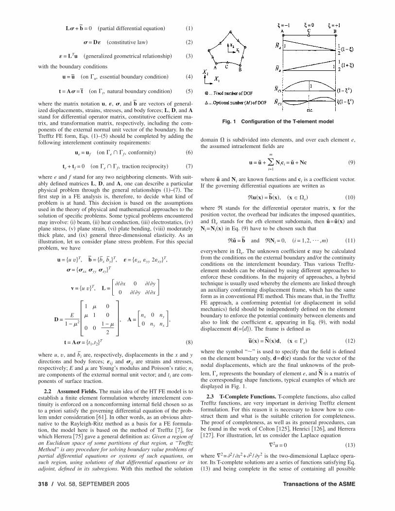
lem, �e represents the boundary of element e, and N is a matrix ofthe corresponding shape functions, typical examples of which aredisplayed in Fig. 1.

2.3 T-Complete Functions. T-complete functions, also calledTrefftz functions, are very important in deriving Trefftz elementformulation. For this reason it is necessary to know how to con-struct them and what is the suitable criterion for completeness.The proof of completeness, as well as its general procedures, canbe found in the work of Colton �125�, Henrici �126�, and Herrera�127�. For illustration, let us consider the Laplace equation

�2u = 0 �13�

where �2=�2 /�x2+�2 /�y2 is the two-dimensional Laplace opera-tor. Its T-complete solutions are a series of functions satisfying Eq.

Fig. 1 Configuration of the T-element model

�13� and being complete in the sense of containing all possible

Transactions of the ASME

solutions in a given solution domain. It can be shown that any ofthe following functions satisfies Eq. �13�:

1,r cos �, r sin �, ¯ , rm cos m�, rm sin m�,¯ �14�

where r and � are a pair of polar coordinates. As a consequence,the so-called T-complete set, denoted by T, can be written as

T = �1,rm cos m�,rm sin m�� = �Ti� �15�

2.4 Variational Principles. The Trefftz FE equation for theboundary value problem �1�–�7� can be established by the varia-tional approach �61�. Since the stationary conditions of the tradi-tional potential and complementary variational functional may notsatisfy the interelement continuity condition, which is required inTrefftz FE analysis, several variants of modified variational func-tionals have been used in the literature to establish Trefftz FEequation. We list here three of them that have been widely used innumerical analysis as below.

1. The two variational principles below were due to Herrera�75,82� and Herrera et al. �83� and are applicable to any boundaryvalue problems. The first one is in terms of the “prescribed data”

�

wRudx − �

��u,w�dx − �

T�u,w�dx = �

fwdx − �

gwdx

− �

jwdx ∀ w � D �16�

while the second one is in terms of the “sought information”

�

uR*wdx − �

C*�u,w�dx − �

K*�u,w�dx = �

fwdx

− �

gwdx − �

jwdx ∀ w � D �17�

where R* is a formal adjoint of R in an abstract sense defined in�82�, ��u ,w� and C*�u ,w� are boundary operators, while T�u ,w�and K*�u,w� are, respectively, the jump and average operators, �stands for the internal boundary, f is body force, g is generalizedboundary force, and j is the force related to discontinuities �see�75,82� for a more detailed explanation on these symbols�. Thevariational principles �16� and �17� were called “direct” and “in-direct” variational formulations of the original boundary valueproblem, respectively.

2. An alternative variational functional for hybrid-Trefftzdisplacement-type formulation is given by �30�

J�u, v� = �e�−

1

2 �e

ueTbd� −

1

2 �e

teTveds +

�e*

teTveds

− �e

teTveds� = stationary �18�

The boundary �e of the element e consists of the following parts:

�e = �eS + �eu + �e + �Ie = �eS + �e* �19�

in which �eS is the portion of �e on which the prescribed bound-ary conditions are satisfied a priori �this is the case when thespecial purpose trial functions are used in the element�, �eu and�e are portions of the remaining part, �e−�eS, of the elementboundary on which either displacement �v= v� or traction �t= t� isprescribed, while �Ie is the interelement portion of �e.

3. The following modified variational functional will be used
throughout this paper �61�:

m = �e

me = �e�e +

�te

�t − t�uds − �Ie

tuds� �20�

�m = �e

�me = �e��e +

�ue

�u − u�tds − �Ie

tuds��21�

where

e = �e

��d� − �ue

tuds �22�

�e = �e

�� − bu�d� − �te

tuds �23�

with

�� = 12�TC�, �� = 1

2�TD� �24�

in which C=D−1 and Eq. �1� are assumed to be satisfied a priori.The term “modified principle” refers here to the use of a conven-tional functional and some modified terms for the construction ofa special variational principle to account for additional require-ments, such as the condition defined in Eqs. �6� and �7�.

The boundary �e of a particular element consists of the follow-ing parts:

�e = �ue � �te � �Ie �25�

where

�ue = �u � �e, �te = �t � �e, �26�

and �Ie is the interelement boundary of the element e. The sta-tionary condition of the functional �20� or �21� and the theorem onthe existence of extremum of the functional, which ensures that anapproximate solution can converge to the exact one, was dis-cussed by Qin �61�.

2.5 Generation of Element Stiffness Matrix. The elementmatrix equation can be generated by setting �me=0 or ��me=0. By reason of the solution properties of the intraelement trialfunctions, the functional me in Eq. �20� can be simplified to

me =1

2 �e

ubd� +1

2 �e

tuds + �te

�t − t�uds − �Ie

tuds

− �ue

tuds �27�

Substituting the expressions given in Eqs. �9� and �12� into �20�and using Eqs. �2�, �3�, and �5� produces

me = − 12cTHc + cTSd + cTr1 + dTr2 + terms without c or d

�28�

in which the matrices H ,S and the vectors r1 ,r2 are all known�61�.

To enforce interelement continuity on the common elementboundary, the unknown vector c should be expressed in terms ofnodal degrees of freedom d. An optional relationship between cand d in the sense of variation can be obtained from

�me

�cT = − Hc + Sd + r1 = 0 �29�

This leads to


¯

c = Gd + g �30�

where G=H−1S and g=H−1r1, and then straightforwardly yieldsthe expression of me only in terms of d and other known matri-ces

me = 12dTGTHGd + dT�GTHg + r2� + terms without d �31�

Therefore, the element stiffness matrix equation can be ob-tained by taking the vanishing variation of the functional me as

�me

�dT = 0 ⇒ Kd = P �32�

where K=GTHG and P=−GTHg−r2 are, respectively, the ele-ment stiffness matrix and the equivalent nodal flow vector. Theexpression �32� is the elemental stiffness matrix equation for Tr-efftz FE analysis.

3 Potential ProblemsThis section is concerned with the application of the HT FE to

the solution of steady potential flow problems. By steady potentialproblems we mean those governed by the Laplace, Poisson, orHelmholtz equations. The method presented is based on a modi-fied variational principle and the T-complete functions discussedin Sec. 2.

3.1 Basic Equations and Assumed Fields. Consider that we

are seeking to find the solution of a Poisson �or Laplace for b=0 below� equation in a domain �

�2u = b �in �� 33�

with b a known function and with boundary conditions

u = u �on �u� �34�

qn =�u

�n= qn �on �q� �35�

where n is the normal to the boundary, �=�u+�q and the dashesindicate that those variables are known.

By way of the method of variable separation, the completesolutions in a bounded region are obtained as �43�

u�r,�� = �m=0

rm�am cos m� + bm sin m�� 36�

for two-dimensional problems and

u�r,�� = �m=0

amrmPmq �cos ��eiq� �37�

for three-dimensional problems, where Pmq �cos �� is the associated

Legendre function, −m�q�m, and the spherical coordinates�r ,� ,�� are used in Eq. �37�. The complete solutions in an un-bounded region can be similarly obtained �61�. Thus, the associ-ated T-complete sets of Eqs. �36� and �37� can be expressed in theform

T = �1,rm cos m�,rm sin m�� = �Ti� �38�

T = �rmPmq �cos ��eiq�� = �Ti� �39�

The internal trial function Nj �j=1,2…m� in Eq. �9� are in thiscase obtained by a suitably truncated T-complete solution �38� or�39�. For example,

N1 = r cos �, N2 = r sin �, N3 = r2 cos 2�,… , �40�

for a two-dimensional problem with a bounded domain. Note that
the function N1=1 is not used here, as it represents rigid body

motion and yields zero element stiffness �this is discussed, in de-tail, in Sec. 3.7�. The particular solution u for any right-hand side

b can be obtained by integration of the source �or Green’s� func-tion �61�

u*�rPQ� =1

2�ln� 1

rPQ� �41�

where P designates the field point under consideration, Q standsfor the source point, and

rPQ = ��xQ − xP�2 + �yQ − yP�2 �42�

The Green’s function u*�rPQ� is the solution for the Laplaceequation in an infinite domain and with a unit potential applied ata given point Q, i.e.,

�2u* = ��P,Q� �43�

where ��P ,Q� is a Dirac � function representing a unit concen-trated potential acting at a point Q. As a consequence, the particu-lar solution u in Eq. �9� can be expressed as

u�P� =1

2�

�e

b�Q�ln� 1

rPQ�d��Q� �44�

The corresponding outward normal derivative of u �“traction”�on �e of element e is

t = qn =�u

�n= qn + �

j=1

m

Tjcj = qn + Qc �45�

3.2 Modified Variational Principle and Element MatrixEquation. The HT FE for potential problems can be establishedby means of a modified variational functional �which is slightlydifferent from that of Chap. 2 in �61��

me = −1

2 �

bud � +1

2 �e

qnuds − �eu

qnuds

+ �eq

�qn − qn�uds − �Ie

qnuds �46�

where �e=�eu+�eq+�Ie, with �eu=�e��u, �eq=�e��q, and �Ieis the interelement boundary of element e. Substituting the expres-sions given in Eqs. �9�, �12�, and �45� into �46� yields Eq. �28�.The matrices H ,S and the vectors r1 ,r2 appeared in Eq. �28� arenow defined by

H = − �e

QTNds �47�

S = − �Ie

QTNds − �eq

QTNds �48�

r1 = −1

2 �e

NTbd� +1

2 �e

�qneNT + QTue�ds −

�eu

QTuds

�49�

r2 = − �Ie

NTqneds + �eq

NT�qn − qne�ds �50�

The element stiffness matrix equation is the same as Eq. �32�.

3.3 Special Purpose Functions. Singularities induced by lo-cal defects, such as angular corners, cracks, etc., can be accurately
accounted for in the conventional FE model by way of appropriate

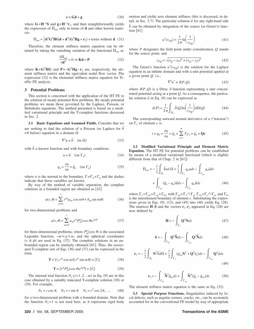
local refinement of the element mesh. However, an important fea-ture of the Trefftz FE method is that such problems can be farmore efficiently handled by the use of special purpose functions�30�. Elements containing local defects �see Fig. 2� are treated bysimply replacing the standard regular functions N in Eq. �9� byappropriate special-purpose functions. One common characteristicof such trial functions is that it is not only the governing differ-ential equations, which are Poisson equations here, which are sat-isfied exactly, but also some prescribed boundary conditions at aparticular portion �eS �see Fig. 2� of the element boundary. Thisenables various singularities to be specifically taken into accountwithout troublesome mesh refinement. Since the whole elementformulation remains unchanged �except that now the frame func-tion u in Eq. �12� is defined and the boundary integration is per-formed at the portion �e* of the element boundary �e=�e* +�eSonly, see Fig. 2�, all that is needed to implement the elementscontaining such special trial functions is to provide the elementsubroutine of the standard, regular elements with a library of vari-ous optional sets of special purpose functions.

The special purpose functions for such a singular corner hasbeen given �p. 56 in �61�� as

u�r,�� = a0 + �n=1

anrn�/�0 cos�n�

�0�� + �

n=1,3,5

dnrn�/2�0 sin� n�

2�0��51�

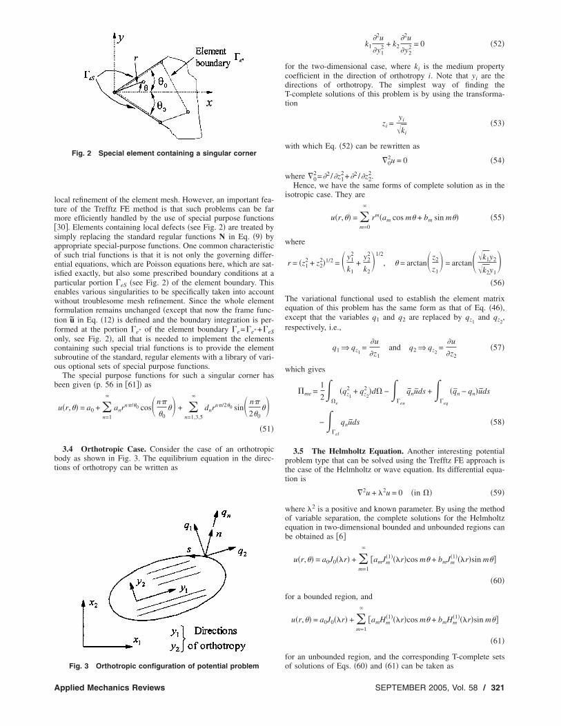
3.4 Orthotropic Case. Consider the case of an orthotropicbody as shown in Fig. 3. The equilibrium equation in the direc-tions of orthotropy can be written as

Fig. 2 Special element containing a singular corner

Fig. 3 Orthotropic configuration of potential problem


k1�2u

�y12 + k2

�2u

�y22 = 0 �52�

for the two-dimensional case, where ki is the medium propertycoefficient in the direction of orthotropy i. Note that yi are thedirections of orthotropy. The simplest way of finding theT-complete solutions of this problem is by using the transforma-tion

zi =yi

�ki

�53�

with which Eq. �52� can be rewritten as

�02u = 0 �54�

where �02=�2 /�z1

2+�2 /�z22.

Hence, we have the same forms of complete solution as in theisotropic case. They are

u�r,�� = �m=0

rm�am cos m� + bm sin m�� 55�

where

r = �z12 + z2

2�1/2 = � y12

k1+

y22

k2�1/2

, � = arctan� z2

z1� = arctan��k1y2

�k2y1�

�56�

The variational functional used to establish the element matrixequation of this problem has the same form as that of Eq. �46�,except that the variables q1 and q2 are replaced by qz1

and qz2,

respectively, i.e.,

q1 ⇒ qz1=

�u

�z1and q2 ⇒ qz2

=�u

�z2�57�

which gives

me =1

2 �e

�qz1

2 + qz2

2 �d� − �eu

qnuds + �eq

�qn − qn�uds

− �el

qnuds �58�

3.5 The Helmholtz Equation. Another interesting potentialproblem type that can be solved using the Trefftz FE approach isthe case of the Helmholtz or wave equation. Its differential equa-tion is

�2u + �2u = 0 �in �� 59�

where �2 is a positive and known parameter. By using the methodof variable separation, the complete solutions for the Helmholtzequation in two-dimensional bounded and unbounded regions canbe obtained as �6�

u�r,�� = a0J0��r� + �m=1

�amJm�1��r�cos m� + bmJm

�1��r�sin m��

�60�

for a bounded region, and

u�r,�� = a0J0��r� + �m=1

�amHm�1��r�cos m� + bmHm

�1��r�sin m��

�61�

for an unbounded region, and the corresponding T-complete sets
of solutions of Eqs. �60� and �61� can be taken as

T = �J0��r�,Jm��r�cos m�,Jm��r�sin m�� = �Ti� �62�

T = �H0�1��r�,Hm

�1��r�cos m�,Hm�1��r�sin m�� = �Ti� �63�

in which Jm��r� and Hm�1��r� are the Bessel and Hankel functions

of the first kind, respectively. As an illustration, the internal func-tion Nj in Eq. �9� can be given in the form

N1 = J0��r�, N2��r� = J1��r�cos �, N3 = J1��r�sin �,¯

�64�

for two-dimensional Helmholtz equations with bounded regions.For a particular element, say element e, the variational functionalused for generating the element matrix equation of this problem is

me =1

2 �e

�q12 + q2

2 − �2u2�d� − �eu

qnuds + �eq

�qn − qn�uds

− �el

qnuds �65�

Before concluding this subsection, we would like to mentionedthat, for Helmholtz equation, Sanchez et al. �128� have shown thata suitable system of plane waves is TH-complete in any boundedregion. This is a TH-complete system which, because of its sim-plicity, could be advantageously used for implementing Trefftzmethod.

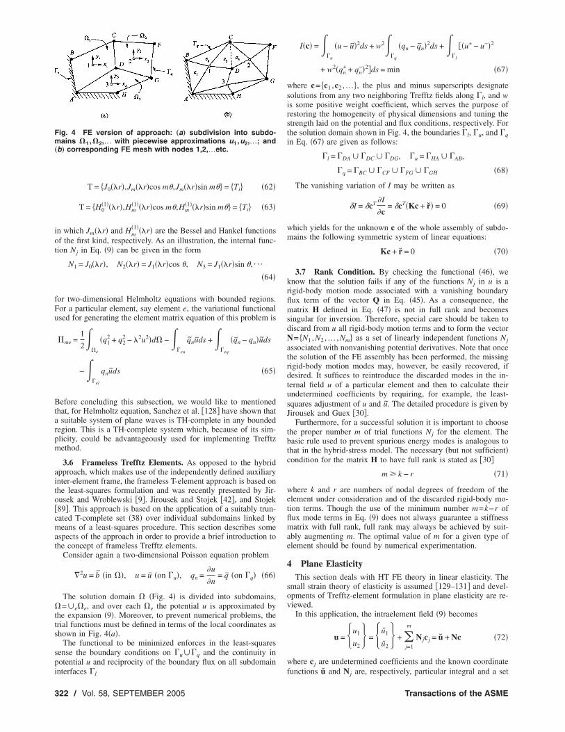
3.6 Frameless Trefftz Elements. As opposed to the hybridapproach, which makes use of the independently defined auxiliaryinter-element frame, the frameless T-element approach is based onthe least-squares formulation and was recently presented by Jir-ousek and Wroblewski �9�. Jirousek and Stojek �42�, and Stojek�89�. This approach is based on the application of a suitably trun-cated T-complete set �38� over individual subdomains linked bymeans of a least-squares procedure. This section describes someaspects of the approach in order to provide a brief introduction tothe concept of frameless Trefftz elements.

Consider again a two-dimensional Poisson equation problem

�2u = b �in ��, u = u �on �u�, qn =�u

�n= q �on �q� �66�

The solution domain � �Fig. 4� is divided into subdomains,�=�e�e, and over each �e the potential u is approximated bythe expansion �9�. Moreover, to prevent numerical problems, thetrial functions must be defined in terms of the local coordinates asshown in Fig. 4�a�.

The functional to be minimized enforces in the least-squaressense the boundary conditions on �u��q and the continuity inpotential u and reciprocity of the boundary flux on all subdomain

Fig. 4 FE version of approach: „a… subdivision into subdo-mains �1 ,�2,… with piecewise approximations u1 ,u2,…; and„b… corresponding FE mesh with nodes 1,2,…etc.

interfaces �l


I�c� = �u

�u − u�2ds + w2 �q

�qn − qn�2ds + �l

��u+ − u−�2

+ w2�qn+ + qn

−�2�ds = min �67�

where c= �c1 ,c2 ,…�, the plus and minus superscripts designatesolutions from any two neighboring Trefftz fields along �l, and wis some positive weight coefficient, which serves the purpose ofrestoring the homogeneity of physical dimensions and tuning thestrength laid on the potential and flux conditions, respectively. Forthe solution domain shown in Fig. 4, the boundaries �l, �u, and �qin Eq. �67� are given as follows:

�l = �DA � �DC � �DG, �u = �HA � �AB,

�q = �BC � �CF � �FG � �GH �68�

The vanishing variation of I may be written as

�I = �cT �I

�c= �cT�Kc + r� = 0 �69�

which yields for the unknown c of the whole assembly of subdo-mains the following symmetric system of linear equations:

Kc + r = 0 �70�

3.7 Rank Condition. By checking the functional �46�, weknow that the solution fails if any of the functions Nj in u is arigid-body motion mode associated with a vanishing boundaryflux term of the vector Q in Eq. �45�. As a consequence, thematrix H defined in Eq. �47� is not in full rank and becomessingular for inversion. Therefore, special care should be taken todiscard from u all rigid-body motion terms and to form the vectorN= �N1 ,N2 ,… ,Nm� as a set of linearly independent functions Njassociated with nonvanishing potential derivatives. Note that oncethe solution of the FE assembly has been performed, the missingrigid-body motion modes may, however, be easily recovered, ifdesired. It suffices to reintroduce the discarded modes in the in-ternal field u of a particular element and then to calculate theirundetermined coefficients by requiring, for example, the least-squares adjustment of u and u. The detailed procedure is given byJirousek and Guex �30�.

Furthermore, for a successful solution it is important to choosethe proper number m of trial functions Nj for the element. Thebasic rule used to prevent spurious energy modes is analogous tothat in the hybrid-stress model. The necessary �but not sufficient�condition for the matrix H to have full rank is stated as �30�

m � k − r �71�

where k and r are numbers of nodal degrees of freedom of theelement under consideration and of the discarded rigid-body mo-tion terms. Though the use of the minimum number m=k−r offlux mode terms in Eq. �9� does not always guarantee a stiffnessmatrix with full rank, full rank may always be achieved by suit-ably augmenting m. The optimal value of m for a given type ofelement should be found by numerical experimentation.

4 Plane ElasticityThis section deals with HT FE theory in linear elasticity. The

small strain theory of elasticity is assumed �129–131� and devel-opments of Trefftz-element formulation in plane elasticity are re-viewed.

In this application, the intraelement field �9� becomes

u = �u1

u2� = �u1

u2� + �

j=1

m

N jc j = u + Nc �72�

where c j are undetermined coefficients and the known coordinate˘
functions u and N j are, respectively, particular integral and a set

of appropriate homogeneous solutions to the equation

LDLTu + b = 0 �on �e� �73�

and

LDLTN j = 0 �on �e� �74�

where b, L, and D are defined in Eq. �8� for plane stress problems.For plane strain applications, it suffices to replace E and � aboveby

E* =E

1 − �2 , �* =�

1 − ��75�

In the presence of constant body forces �b1 and b2 being twoconstants�, the particular solution is conveniently taken as

u = −1 + �

E �b1y2

b2x2� �76�

The distribution of the frame �12� can now be written as

u1 = NAu1A + NBu1B + �i=1

M

�i−1NCiaCi �77�

u2 = NAu2A + NBu2B + �i=1

M

�i−1NCibCi �78�

along a particular side A-C-B of an element �Fig. 1�, where NA,

NB and NCi are defined in Fig. 1, � is a coefficient equal to either1 or −1 according to the orientation of the side A-C-B �Fig. 1� inthe global coordinate system �X1 ,X2�

� = �+ 1 if X1B − X1A � X2B − X2A

− 1 otherwise� �79�

A T-complete set of homogeneous solutions N j can be gener-ated in a systematic way from Muskhelishvili’s complex variableformulation �132�. They can be written as �25�

2GNej = �Re Z1k

Im Z1k� with Z1k = i�zk + kizzk−1 �80�

2GNej+1 = �Re Z2k

Im Z2k� with Z2k = �zk − kzzk−1 �81�

2GNej+2 = �Re Z3k

Im Z3k� with Z3k = izk �82�

2GNej+3 = �Re Z4k

Im Z4k� with Z4k = − zk �83�

The corresponding stress field is obtained by the standard consti-tutive relation �2�

� = ��11

�22

�12� = � + �

j=1

m

T jc j = � + Tc �84�

while the particular solution � can be easily obtained by setting�=DLTu. Derivation of the element stiffness equation is based on
the functional

me =1

2 �e

�LTu�TDLTud� − �eu

tuds + �e

�t − t�uds

− �el

tuds �85�

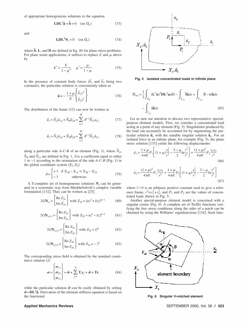
Let us turn our attention to discuss two representative special-purpose element models. First, we consider a concentrated loadacting at a point of any element �Fig. 5�. Singularities produced bythe load can accurately be accounted for by augmenting the par-ticular solution ue with the suitable singular solution ue. For anisolated force in an infinite plane, for example �Fig. 5�, the planestress solution �133� yields the following displacements:

u1 =1 + �

4�EP1��1 + ��

x12

r2 −3 − �

2ln

r2

l2� +�1 + ��2

4�EP2

x1x2

r2

�86�

u2 =�1 + ��2

4�EP1

x1x2

r2 +1 + �

4�EP2��1 + ��

x22

r2 −3 − �

2ln

r2

l2��87�

where l�0 is an arbitrary positive constant used to give a refer-ence frame, r2=x1

2+x22, and P1 and P2 are the values of concen-

trated loads shown in Fig. 5.Another special-purpose element model is concerned with a

singular corner �Fig. 6�. A complete set of Trefftz functions veri-fying the free stress conditions along the sides of a notch can beobtained by using the Williams’ eigenfunctions �134�. Such func-

Fig. 5 Isolated concentrated loads in infinite plane

Fig. 6 Singular V-notched element


tions have, in the past, been used successfully by Lin and Tong�135� to generate a singular V-notched superelement. These func-tions can be used to generate special-purpose elements with sin-gular corners. They are

2Gu1 = a�n

Re�� r

a��n

�n�� + �n cos 2� + cos 2�n��cos �n�

− �n cos��n − 2�� − � r

a��n

�n�� + �n cos 2� − cos 2�n��

�sin �n� − �n sin��n − 2�� 88�

2Gu2 = a�n

Re�� r

a��n

�n�� − �n cos 2� − cos 2�n��sin �n�

+ �n sin��n − 2�� + � r

a��n

�n�� − �n cos 2� + cos 2�n��

�cos �n� + �n cos��n − 2�� 89�

where a is defined by

a = �i=1

N�x1i

2 + x2i2 �1/2

N�90�

with N being the number of nodes in the element under consider-ation, �n and �n are real undetermined constants, � and � areshown in Fig. 6, while �n and �n are eigenvalues that have a realpart greater than or equal to 1/2 and are the roots of the followingcharacteristic equations:

sin 2�n� = − �n sin 2� �91�

for symmetric �tension� loading, and

sin 2�n� = �n sin 2� �92�

for antisymmetric �pure shear� loading.Apart from their high efficiency in solving singular corner

problems, the great advantage of the above special-purpose func-tion set is the attractive possibility of straightforwardly evaluatingthe stress intensity factors KI �opening mode� and KII �slidingmode� from the first two internal parameters �1 and �1

KI = �2��1a1−�1��1 + 1 − �1 cos 2� − cos 2�1��1 �93�

KII = �2��1a1−�1��1 − 1 − �1 cos 2� + cos 2�1��1 �94�

5 Thin Plate BendingIn Secs 3 and 4, applications of Trefftz-elements to the potential

problem and plane elasticity were reviewed. Extension of the pro-cedure to thin plate bending is briefly reviewed in this section.

For thin-plate bending the equilibrium equation and its bound-ary conditions are well established in the literature �e.g., �61��.

In the case of a thin-plate element the internal displacementfield �9� becomes

w = w + �j=1

m

Njcj = w + Nc �95�

where w is the transverse deflection, w and Nj are known func-tions, which should be chosen so that

D�4w = q and �4Nj = 0, �j = 1,2, ¯ ,m� �96�

everywhere in the element sub-domain �e, where q is the distrib-4 4 4 4 2 2 4 4
uted vertical load per unit area, � =� /�x1+2� /�x1�x2+� /�x2

is the biharmonic operator, and D=Et3 /12�1−�2�. In the hybridapproach under consideration, the elements are linked through anauxiliary displacement frame

v = � w

w,n� = �N1

N2

�d = Nd �97�

where d stands for the vector of nodal parameters and N is theconventional finite element interpolating matrix such that the cor-responding nodal parameters of the adjacent elements arematched. Based on the approach of variable separation, theT-complete solution of the biharmonic equation, D�4w= q, can befound �108,127�

w = �n=0

�Re��an + r2bn�zn� + Im��cn + r2dn�zn�� 98�

where

r2 = x12 + x2

2, z = x1 + ix2 �99�

Hence, the T-complete system for plate-bending problems canbe taken as

T = �1,r2,Re z2,Im z2,r2 Re z,r2 Im z,Re z3, ¯ � �100�

The Trefftz FE formulation for thin-plate bending can be derivedby means of a modified variational principle �e.g., �22��. The re-lated functional used for deriving the HT element formulation isconstructed as

m = �e�e −

�e2

�Mn − Mn�w,nds + �e4

�R − R�wds

+ �e5

�Mnw,n − Rw�ds� �101�

where

e = �e

Ud� + �e1

Mnw,nds − �e3

Rwds �102�

with

U =1

2D�1 − �2��M11 + M22�2 + 2�1 + ��M12

2 − M11M22��

�103�

The boundary �e of a particular element consists of the follow-ing parts:

�e = �e1 + �e2 + �e5 = �e3 + �e4 + �e5 �104�

where

�e1 = �e � �wn,�e2 = �e � �M,�e3 = �e � �w,�e4 = �e � �R

�105�

and �e5 is the interelement boundary of the element.The formulation described above can be extended to the case of

thin plates on an elastic foundation. In this case, the left-hand sideof the equation D�4w= q and the related plate boundary equation,

Mn=Mijninj =Mn, must be augmented by the terms Kw and−�Gpw, respectively:

D�4w + Kw = q �in �� 106�

Mn = Mijninj − �Gpw = Mn �on �M� �107�

where �=0 for a Winkler-type foundation, �=1 for a Pasternak-
type foundation, and the reaction operator

K = �kw for a Winkler-type foundation

�kp − Gp�2� for a Pasternak-type foundation

��108�

with kw being the coefficient of a Winkler-type foundation, and kPand GP being the coefficient and shear modulus of a Pasternak-type foundation. The T-complete functions for this problem are�61�

f�r,�� = a0f0�r� + �m=1

�amfm�r�cos m� + bmfm�r�sin m��

�109�

where fm�r�= Im�r�C2�−Jm�r�C1� and the associated internalfunction Nj can be taken as

N1 = f0�r�, N2m = fm�r�cos m�, N2m+1 = fm�r�sin m�

�m = 1,2, ¯ � �110�

in which Im�� and Jm�� are, respectively, modified and standardBessel function of the first kind with order m, and

C1 = C2 = i�kw/D �111�

for a Winkler-type foundation, and

C1 = −GP

2D−��GP

2D�2

−kP

D, C2 =

GP

2D−��GP

2D�2

−kP

D

�112�

for a Pasternak-type foundation, and i=�−1.The variational functional used for deriving HT FE formulation

of thin plates on an elastic foundation has the same form as that ofEq. �101�, except that the complementary energy density U in Eq.�103� is replaced by U*

U* =1

2D�1 − �2��M11 + M22�2 + 2�1 + ��M12

2 − M11M22�� + V*

�113�

where

V* = � kww2

2for a Winkler-type foundation

12 �kPw2 + GPw,iw,i� for a Pasternak-type foundation

��114�

6 Thick-Plate ProblemsBased on the Trefftz method, Petrolito �37,38� presented a hi-

erarchic family of triangular and quadrilateral Trefftz elements foranalyzing moderately thick Reissner-Mindlin plates. In these HTformulations, the displacement and rotation components of the

auxiliary frame field u= �w , �x , �y�T, used to enforce conformityon the internal Trefftz field u= �w ,�x ,�y�T, are independently in-terpolated along the element boundary in terms of nodal values.Jirousek et al. �34� showed that the performance of the HT thick-plate elements could be considerably improved by the applicationof a linked interpolation whereby the boundary interpolation ofthe displacement w is linked through a suitable constraint with

that of the tangential rotation component �s. This concept, intro-duced by Xu �136�, has been applied recently by several research-ers to develop simple and well-performing thick-plate elements�33,34,137–140�. In contrast to thin-plate theory as described inthe previous section, Reissner-Mindlin theory �141,142� incorpo-rates the contribution of shear deformation to the transverse de-
flection. In Reissner-Mindlin theory, it is assumed that the trans-

verse deflection of the middle surface is w, and that straight linesare initially normal to the middle surface rotate �x about they-axis and �y about the x-axis. The variables �w ,�x ,�y� are con-sidered to be independent variables and to be functions of x and yonly. A convenient matrix form of the resulting relations of thistheory may be obtained through use of the following matrix quan-tities:

u = �w,�x,�y�T �generalized displacement� �115�

� = ��x �y �xy �x �y�T = LTu �generalized strains� �116�

� = �− Mx − My − Mxy Qx Qy�T = D� �generalized stresses��117�

t = �Qn − Mnx − Mny�T = A� �generalized boundary tractions��118�

where L, D, and A are defined by

L = 0 0 0

�

�x

�

�y

�

�x0

�

�y− 1 0

0�

�y

�

�x0 − 1

, A = 0 0 0 nx ny

nx 0 ny 0 0

0 ny nx 0 0 ,

D = �DM 0

0 DQ�

DM =Et3

12�1 − �2�1 � 0

� 1 0

0 01 − �

2, DQ =

Etk

2�1 + ��1 0

0 1�

�119�

with k being a correction factor for nonuniform distribution ofshear stress across thickness t, which is usually taken as 5/6.

The governing differential equations of moderately thick platesare obtained if the differential equilibrium conditions are writtenin terms of u as

L� = LDLTu = b �120�

where the load vector

b = �q mx my�T �121�

comprises the distributed vertical load in the z direction and thedistributed moment loads about the y- and x-axes �the bar abovethe symbols indicates imposed quantities�.

The corresponding boundary conditions are given by

a. simply supported condition

w = w �on �w�, �s = �isi = �s �on ��s�,

Mn = Mijninj = Mn �on �Mn� �122�

b. clamped condition

w = w �on �w�, �s = �s �on ��s�,

�n = �ini = �n �on ��n� �123�

c. free-edge conditions


Mn = Mn �on �Mn�, Mns = Mns �on �Mns

�,

Qn = Qini = Qn �on �Q� �124�

where n and s are, respectively, unit vectors outward normal andtangent to the plate boundary ��=��n

��Mn=��s

��Mns=�w��Q�.

The internal displacement field in a thick plate is given in Eq.�9�, in which u and N j are, respectively, the particular and homo-geneous solutions to the governing differential equations �120�,namely,

LDLTu = b and LDLTN j = 0, �j = 1,2, ¯ ,m� �125�

To generate the internal function N j, consider again the governingequations �120� and write them in a convenient form as

D� �2�x

�x2 +1 − �

2

�2�x

�y2 +1 + �

2

�2�y

�x � y� + C� �w

�x− �x� = 0

�126�

D� �2�y

�y2 +1 − �

2

�2�y

�x2 +1 + �

2

�2�x

�x � y� + C� �w

�y− �y� = 0

�127�

C��2w −��x

�x−

��y

�y� = q �128�

where

D =Et3

12�1 − �2�, C

5Et

12�1 + ��129�

and where, for the sake of simplicity, vanishing distributed mo-ment loads, mx= my =0, have been assumed.

The coupling of the governing differential equations�126�–�128� makes it difficult to generate a T-complete set of ho-mogeneous solutions for w, �x, and �y. To bypass this difficulty,two auxiliary functions f and g are introduced �143� such that

�x = g,x + f ,y and �y = g,y − f ,x �130�

It should be pointed out that

g0,x + f0,y = 0 and g0,y − f0,x = 0 �131�

are Cauchy-Riemann equations, the solution of which always ex-ists. As a consequence, �x and �y remain unchanged if f and g inEq. �130� are replaced by f + f0 and g+g0. This property plays animportant part in the solution process. Using these two auxiliaryfunctions, Eq. �126�–�128� is converted as the form

D�4g = p and �2f − �2f = 0 �132�

with �2=10�1−�� / t2.The relations �132� are the biharmonic equation and the modi-

fied Bessel equation, respectively. Their T-complete solutions are

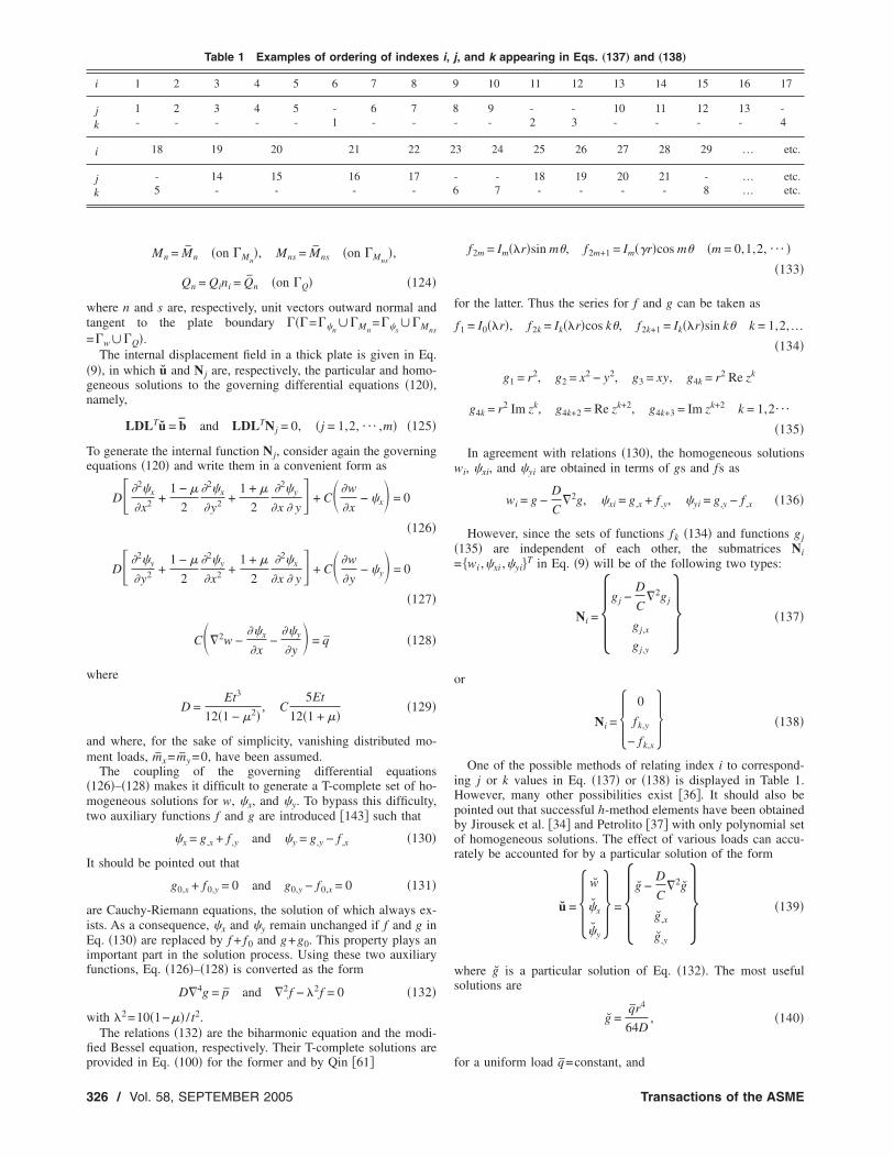
Table 1 Examples of ordering of indexes

i 1 2 3 4 5 6 7 8

j 1 2 3 4 5 - 6 7k - - - - - 1 - -

i 18 19 20 21 22

j - 14 15 16 17k 5 - - - -

provided in Eq. �100� for the former and by Qin �61�


f2m = Im��r�sin m�, f2m+1 = Im��r�cos m� �m = 0,1,2, ¯ ��133�

for the latter. Thus the series for f and g can be taken as

f1 = I0��r�, f2k = Ik��r�cos k�, f2k+1 = Ik��r�sin k� k = 1,2,…�134�

g1 = r2, g2 = x2 − y2, g3 = xy, g4k = r2 Re zk

g4k = r2 Im zk, g4k+2 = Re zk+2, g4k+3 = Im zk+2 k = 1,2¯

�135�

In agreement with relations �130�, the homogeneous solutionswi, �xi, and �yi are obtained in terms of gs and fs as

wi = g −D

C�2g, �xi = g,x + f ,y, �yi = g,y − f ,x �136�

However, since the sets of functions fk �134� and functions gj�135� are independent of each other, the submatrices Ni= �wi ,�xi ,�yi�T in Eq. �9� will be of the following two types:

Ni = �gj −D

C�2gj

gj,x

gj,y

� �137�

or

Ni = � 0

fk,y

− fk,x� �138�

One of the possible methods of relating index i to correspond-ing j or k values in Eq. �137� or �138� is displayed in Table 1.However, many other possibilities exist �36�. It should also bepointed out that successful h-method elements have been obtainedby Jirousek et al. �34� and Petrolito �37� with only polynomial setof homogeneous solutions. The effect of various loads can accu-rately be accounted for by a particular solution of the form

u = � w

�x

�y

� = �g −D

C�2g

g,x

g,y

� �139�

where g is a particular solution of Eq. �132�. The most usefulsolutions are

g =qr4

64D, �140�

¯

j, and k appearing in Eqs. „137… and „138…

10 11 12 13 14 15 16 17

9 - - 10 11 12 13 -- - 2 3 - - - - 4

3 24 25 26 27 28 29 … etc.

- - 18 19 20 21 - … etc.7 - - - - 8 … etc.

i,

9

8

2

6

for a uniform load q=constant, and


g =PrPQ

2

8�Dln rPQ, �141�

for a concentrated load P, where rPQ is defined in Sec. 3. Anumber of particular solutions for Reissner-Mindlin plates can befound in standard texts �e.g., Reismann �144��.

Since evaluation of the element matrices calls for boundaryintegration only �see Sec. 3, for example�, explicit knowledge ofthe domain interpolation of the auxiliary conforming field is notnecessary. As a consequence, the boundary distribution of u

= Nd, referred to as “frame function,” is all that is needed.The elements considered in this section are either p type �M

�0� �Fig. 1� or conventional type �M =0�, with three standarddegrees of freedom at corner nodes, e.g.,

dA = uA = �wA,�xA,�yA�T, dB = uB = �wB,�xB,�yB�T �142�

and an optional number M of hierarchical degrees of freedomassociated with midside nodes

dC = �uC = ��wC1,��xC1,��yC1,�wC2,��xC2,��yC2, ¯ etc . �T

�143�

Within the thin limit �x=�w /�x and wy =�w /�y, the order of thepolynomial interpolation of w has to be one degree higher thanthat of �x and �y if the resulting element is to be free of shearlocking. Hence, if along a particular side A-C-B of the element�Fig. 1�

�xA-C-B = NA�xA + NB�xB + �i=1

p−1

NCi��xCi �144�

�yA-C-B = NA�yA + NB�yB + �i=1

p−1

NCi��yCi �145�

where NA, NB, and NCi are defined in Fig. 1, p is the polynomial

degree of �x and �y �the last term in Eqs. �144� and �145� will bemissing if p=1�, then the proper choice for the deflection interpo-lation is

wA-C-B = NAwA + NBwB + �i=1

p

NCi�wCi �146�

The application of these functions for p=1 and p=2 along with13 or 25 polynomial homogeneous solutions �137� leads to ele-ments identical to Petrolito’s quadrilaterals Q21-13 and Q32-25�37�.

An alternative variational functional presented by Qin �36� forderiving HT thick-plate elements is as follows:

m = �e�e +

�e2

�Qn − Qn�wds + �e4

�Mn − Mn��nds

+ �e6

�Mns − Mns��sds − �e7

�Mn�n + Mns�s + Qnw�ds��147�

where

e = �e

Ud� − �e1

Qnwds − �e3

Mn�nds − �e5

Mns�sds

�148�

with


U =1

2D�1 − �2��M11 + M22�2 + 2�1 + ��M12

2 − M11M22��

+1

2C�Qx

2 + Qy2� �149�

and where Eqs. �126�–�128� are assumed to be satisfied a priori.The boundary �e of a particular element consists of the followingparts:

�e = �e1 + �e2 + �e7 = �e3 + �e4 + �e7 = �e5 + �e6 + �e7

�150�

where

�e1 = �e � �w, �e2 = �e � �Q, �e3 = �e � ��n,

�e4 = �e � �Mn

�e5 = �e � ��s, �e6 = �e � �Mns

�151�

and �e7 is the interelement boundary of the element.The extension to thick plates on an elastic foundation is similar

to that in Sec. 5. In the case of a thick plate resting on an elasticfoundation, the left-hand side of Eq. �128� and the boundary equa-tion �122� must be augmented by the terms Kw and −�Gpw, re-spectively,

C��2w −��x

�x−

��y

�y� + Kw = q �in �� 152�

Mn = Mijninj − �Gpw = Mn �on �Mn� �153�

where � and K are as defined in Sec. 5.As discussed before, the transverse deflection w and the rota-

tions �x ,�y may be expressed in terms of two auxiliary functions,g and f , by the first part of Eq. �136� and Eq. �130�. The functionf is again obtained as a solution of the modified Bessel equation�second part of Eq. �132��, while for g, instead of the biharmonicequation �first part of Eq. �132��, the following differential equa-tion now applies �36�:

D�4g +K

C�2g − Kg = q �154�

The corresponding T-complete system of homogeneous solu-tions is obtained in a manner similar to that in Sec. 5, as

g�r,�� = c1G0�r� + �j=1

�c2jGj�r�cos j� + c2j+1Gj�r�sin j��

�155�

where

Gj�r� = Ij�r�C2� − Jj�r�C1� �156�

with

C1 =�� kw

2C�2

+kw

D+

kw

2C, C2 =�� kw

2C�2

+kw

D−

kw

2C

�157�

for a Winkler-type foundation and

C1 =�b + kP/C + GP/D

2�1 − GP/C�, C2 =

�b − kP/C − GP/D

2�1 − GP/C��158�

b = � kP

C+

GP

D�2

+4kP

D�1 −

Gp

C� �159�

for a Pasternak-type foundation.


The variational functional used to derive HT FE formulation forthick plates on an elastic foundation is the same as Eq. �147�except that the strain energy function U in Eq. �149� is now re-placed by U*

U* = U + V*, �160�

in which U and V* are defined in Eqs. �149� and �114�, respec-tively.

7 Transient Heat ConductionConsider a two-dimensional heat conduction equation that de-

scribes the unsteady temperature distribution in a solid �domain��. This problem is governed by the differential equation

k�2u + Q = �c�u

�t, �161�

subject to the initial condition in �

u�x,y,0� = u0�x,y� �162�

and the boundary conditions on �

u�x,y,t� = u�x,y,t� �on �1� �163�

p�x,y,t� = p�x,y,t� �on �2� �164�

q�x,y,t� = q�x,y,t� �on �3� �165�

in which

p = k�u

�n, q = hu + p, q = huenv �166�

� = � + �, � = �1 + �2 + �3 �167�

where u�x ,y , t� is the temperature function, Q the body heatsource, k the specified thermal conductivity, � the density, and cthe specific heat. Furthermore, u0 is the initial temperature, h isthe heat transfer coefficient, and uenv stands for environmentaltemperature.

The initial boundary value problem �161�–�165� cannot, in gen-eral, be solved analytically. Hence, the time domain is dividedinto N equal intervals and denoted �t= tm− tm−1. Consider now a

typical time interval �tm , tm+1�, in which u and Q are approximatedby a linear function

u�t� �1

�t��t − tm�um+1 − �t − tm+1�um� �168�

Q�t� �1

�t��t − tm�Qm+1 − �t − tm+1�Qm� �169�

The integral of Eq. �161� over the time interval �tm , tm+1� yields

um+1 = um +�t

2�c�k�2um + k�2um+1 + Qm + Qm+1� �170�

From this we arrive at the following single time-step formula �48�:

��2 − a2�um = bm �171�

with the boundary conditions

um = um �on �1�, pm = pm �on �2�, qm = qm �on �3��172�

where

pm = k�um , qm = hum + pm �173�
�n

a2 =2�c

k�t, bm = − ��2 + a2�um−1 −

1

k�Qm + Qm−1� �174�

and where um, pm, and qm stand for imposed quantities at the timet= tm. Hereafter, to further simplify the writing, we shall omit theindex m appearing in Eqs. �171� and �172�.

Consider again the boundary value problem defined in Eqs.�171�–�174�. The domain is subdivided into elements and overeach element e the assumed field is defined in Eq. �9�, where uand Nj are known functions, which satisfy

��2 − a2�u = b, ��2 − a2�Nj = 0 �on �e� �175�

The second equation of �175� is the modified Bessel equation, forwhich a T-complete system of homogeneous solution can be ex-pressed, in polar coordinates r and �, as

N2m = Im�ar�sin m�, N2m+1 = Im�ar�cos m� �m = 0,1,2, ¯ ��176�

The particular solution u of Eq. �175� for any right-hand side bcan be obtained by integration of the source function

u*�rPQ� =1

2�K0�arPQ� �177�

As a consequence, the particular solution u of Eq. �171� can beexpressed as

u�P� =1

2�

�e

b�Q�K0�arPQ�d��Q� �178�

The area integration in Eq. �178� can be performed by numeri-cal quadrature using the Gauss-Legendre rule.

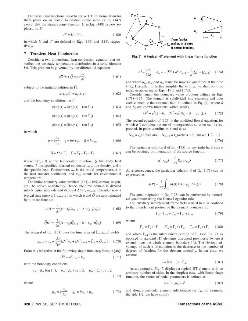
The auxiliary interelement frame field u used here is confinedto the interelement portion of the element boundary �e

�e = �e1 + �e2 + �e4 + �e4 �179�

where

�e1 = �e � �1, �e2 = �e � �2, �e3 = �e � �3 �180�

and where �e4 is the interelement portion of �e �see Fig. 7�, asopposed to standard HT elements discussed previously �where uextends over the whole element boundary �e�. The obvious ad-vantage of such a formulation is the decrease in the number ofdegrees of freedom for the element assembly. In our case, weassume

u = Nd �on �e4� �181�

As an example, Fig. 7 displays a typical HT element with anarbitrary number of sides. In the simplest case, with linear shapefunction, the vector of nodal parameters is defined as

d = �u1, u2, u3�T �182�

and along a particular element side situated on �4e, for example,

Fig. 7 A typical HT element with linear frame function

the side 1-2, we have simply


u = N1u1 + N2u2 �183�

where

N1 = 1 − �12, N2 = �12 �184�

There are no degrees of freedom at nodes 4 and 5 situated on�e�� is the boundary of the domain�.

To enforce the boundary conditions �172� and the interelementcontinuity on u, we minimize for each element the followingleast-squares functional

�e1

�u − u�2ds + d2 �e2

�p − p�2ds + d2 �e3

�q − q�2ds

+ �e4

�u − u�2ds = min �185�

where d�0 is an arbitrary chosen length �in this section d ischosen as the average distance between the element center andelement corners defined in Eq. �3.51� of Qin �61��, which servesthe purpose of obtaining a physically meaningful functional �ho-mogeneity of physical units�. The least-squares statement �185�yields for the internal parameter c the following system of linearequations:

Ac = a + Wd �186�

where

A = �e1��e4

NTNds + d2 �e2

PTPds + d2 �e3

QTQds

�187�

a = �e1

NT�u − u�ds + d2 �e2

PT�p − p�ds + d2 �e3

QT�q − q�ds

�188�

W = �e4

NTNds �189�

From Eqs. �186�–�189�, the internal coefficients c are readilyexpressed in terms of the nodal parameters d

c = c + Cd �190�

where

c = A−1a, C = A−1W �191�

We now address evaluation of the element matrices. In order toenforce “traction reciprocity”

�ue

�ne+

�uf

�nf= 0, �on �e � � f� �192�

and to obtain a symmetric positive definite stiffness matrix, weset, in a similar way as in �63�,

k �e

�u

�n�uds =

�e2

p�uds + �e3

q�uds − h �e4

u�uds + k�dTr

�193�

where r stands for the vector of fictitious equivalent nodal forcesconjugate to the nodal displacement d. This leads to the custom-ary “force-displacement” relationship

r = r + kd �194�

where


r = CT�Hc + h� and k = CTHC �195�

The auxiliary matrices h and H are calculated by setting

�u

�n=

�

�n�u + Nc� = t + Tc �196�

and then performing the following boundary integrals:

h = �e

NTtds −1

k� �e2

NTpds + �e3

NT�s − hu�ds��197�

H = �e

NTTds +h

k �e3

NTNds �198�

Through integration by parts, it is easy to show that the firstintegral in Eq. �198� may be written as

�e

NTTds = �e

BTBds �199�

where

B = � �N

�x,�N

�y�T

�200�

As a consequence, H is a symmetric matrix.

8 Postbuckling Bending of Thin PlateIn this section, the application of HT elements to postbuckling

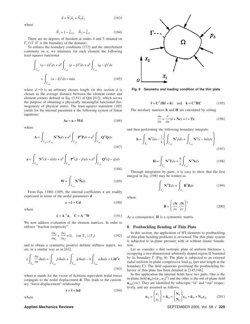
of thin-plate bending problems is reviewed. The thin plate systemis subjected to in-plane pressure with or without elastic founda-tion.

Let us consider a thin isotropic plate of uniform thickness t,occupying a two-dimensional arbitrarily shaped region � boundedby its boundary � �Fig. 8�. The plate is subjected to an externalradial uniform in-plane compressive load p0 �per unit length at theboundary ��. The field equations governing the postbuckling be-havior of thin plate has been detailed in �145,146�.

In this application the internal fields have two parts. One is thein-plane field uin�=�u1 ,u2�T� and the other is the out-of-plane fielduout�=w�. They are identified by subscripts “in” and “out” respec-tively, and are assumed as follows:

u =u1

= u +N1

c = u + N c �201�

Fig. 8 Geometry and loading condition of the thin plate

in �u2� in �

N2� in in in in


uout = w = w + N3cout �202�

where cin and cout are two undetermined coefficient vectors anduin, w, Nin, and N3 are known functions, which satisfy

�L1 L2

L2 L3�uin =� P1

P2

�, �L1 L2

L2 L3��N1

N2� = 0 �in �e�

�203a�

L4w = P3, L4N3 = 0 �in �e� �203b�

and where Li have been defined in �49,61�, Nin and N3 are formedby suitably truncated T-complete systems of the governing equa-tion �61�:

L1u1 + L2u2 = P1

L2u1 + L3u2 = P2

L4w = P3 �204�

The T-complete functions corresponding to the first two lines ofEq. �204� have been given in expressions �80�–�83�, while theTrefftz functions related to the third line of Eq. �204� are �61�

T = �f0�r�, fm�r�cos m�, fm�r�sin m�� = �Ti� �205�

where fm�r�=rm−Jm��r�.All that is left is to determine the parameters c so as to enforce

on u�=�u1 , u2 , w�T� interelement conformity �ue=u f on �e�� f�and the related boundary conditions, where e and f stand for anytwo neighbouring elements. This can be completed by linking theTrefftz-type solutions �201� and �202� through an interface dis-placement frame surrounding the element, which is approximatedin terms of the same degrees of freedom, d, as used in the con-ventional elements

u = Nd �206�

where

u = �uin,uout�T �207�

uin = �u1, u2�T = �N1

N2

�din = Nindin �208�

uout = �w,w,n�T = �N3

N4

�dout = Noutdout �209�

d = �din,dout�T �210�

and where din and dout stand for nodal parameter vectors of the

in-plane and out-of-plane displacements, and Ni= �i=1–4� are theconventional FE interpolation functions.

The particular solutions uin and w in Eq. �201� and �202� areobtained by means of a source-function approach. The sourcefunctions corresponding to Eq. �204� can be found in �146�

uij* �rPQ� =

1 + �

4�E�− �3 − ��ij ln rPQ + �1 + ��rPQ,irPQ,j�

�211�

w*�rPQ� =1

4�D�2 �2 ln rPQ − �Y0��rPQ�� 212�

where uij* �rPQ� represents the ith component of in-plane displace-

ment at the field point P of an infinite plate when a unit point


force �j=1,2� is applied at the source point Q, while w*�rPQ�stands for the deflection at point P due to a unit transverse forceapplied at point Q. Using these source functions, the particularsolutions uin and w can be expressed as

uin = �

Pj�u1j*

u2j* �d� �213�

w = �

P3w*d� �214�

The element matrix equation can be generated by way of follow-ing functionals �61�:

me�in� =1

2 �e

Piuid� − �e1

N˙

nunds − �e3

N˙

nsusds

− �e2

�Nn − Nn*�unds −

�e4

�Nns − Nns* �usds

+1

2 �e

tinuinds − �e9

tinuinds �215�

me�out� =1

2 �e

P3wd� + �e5

M˙

nw,nds − �e7

R˙wds

+ �e6

�Mn − M˙

n�w,nds − �e8

�R − R*�wds

+1

2 �e

toutuoutds − �e9

toutuoutds . �216�

The boundary �e of a particular element here consists of the fol-lowing parts:

�e = �e1 + �e2 + �e9 = �e3 + �e4 + �e9 = �e5 + �e6 + �e9

= �e7 + �e8 + �e9 �217�

where

�e1 = �e � �un, �e2 = �e � �Nn

, �e3 = �e � �us

�e4 = �e � �Nns, �e5 = �e � �wn

, �e6 = �e � �Mn

�e7 = �e � �w, �e8 = �e � �R �218�

and �e9 represents the interelement boundary of the element.Extension to postbuckling plate on an elastic foundation is

similar to the treatment in Sec. 5. In this case the left-hand side of

the third line of Eq. �204� and the boundary equation Mn

=Mijninj =M˙

n must be augmented by the terms Kw and �GPw,respectively,

L4w + Kw = P3 �219�

Mn = Mijninj − �GPw = M˙

n �220�

where �, K, and GP are defined in Sec. 5.The Trefftz functions of Eq. �219� can be obtained by consid-

ering the corresponding homogeneous equation


�L4 + K�g = ��4 + �2�2 + S�g = ��2 + b1��2 + b2�g = 0

�221�

As a consequence, the T-complete system of Eq. �221� is obtainedas �61�

T = �f0�r�, fm�r�sin m�, fm�r�cos m�� = �Ti� �222�

where fm�r�=Jm�r�b1�−Jm�r�b2�, with b1,2=�2��4−4kw /D fora Winkler-type foundation.

9 Geometrically Nonlinear Analyses of Thick PlatesEmployment of Trefftz-element approach enabled Qin �50� and

Qin and Diao �52� to solve for the first time a large deflectionproblem of thick plate with or without elastic foundation. Formu-lations presented in this section are based on the developmentsmentioned above.

Consider a Mindlin-Reissner plate of uniform thickness t, oc-cupying a two-dimensional arbitrarily shaped region � withboundary �. The nonlinear behavior of the plate for moderatelylarge deflection is governed by the following incremental equa-tions �147�:

L1u1 + L2u2 = P1 �223�

L2u1 + L3u2 = P2 �224�

L33w + L34�1 + L35�2 = P3 + q �225�

L43w + L44�1 + L45�2 = 0 �226�

L53w + L54�1 + L55�2 = 0 �227�

together with

un = uini = un �on �un�, us = uisi = us �on �us

� �228�

Nn = Nijl ninj = N

˙n − Nij

n ninj = Nn* �on �Nn

� �229�

Nns = Nijl nisj = N

˙ns − Nij

n nisj = Nns* �on �Nns

� �230�

for in-plane boundary condition and

w = w �on �w�, �n = �ini = �˙

n �on ��n�, �s = �isi = �

˙s �on ��s

�

�231�

for clamped edge, or

w = w �on �w�, �s = �˙

s �on ��s�, Mn = Mijninj = M

˙n �on �Mn

�

�232�

for simply supported edge, or

Mn = M˙

n �on �Mn�, Mns = Mijnisj = M

˙ns �on �Mns

�,

R = Qini = R˙

− Rn = R* �on �R� �233�

for free edge, where Rn=Nnw,n+Nnsw,s, L1 ,L2 ,L3, and P1 , P2 , P3are defined in �61�, q represents the transverse distributed load,and

L33 = C�2, L34�� = − L43�� = − C��,1, L35 = − L53 = − C��,2

L44 = DL1 − C, L45 = L54 = DL2, L55 = DL3 − C �234�


As noted before, the HT FE model is based on assuming twosets of distinct displacements, the internal field u and the framefield u. The internal field u fulfil’s the governing differential equa-tions �223�–�227� identically and is assumed over each element as

u = � uin

uout� = � uin

uout� + �Nin 0

0 Nout�� cin

cout� = u + Nc

�235�

where

uin = �u1, u2�T, uout = �w,�1,�2�T, uin = �u1, u2�T,

uout = �w,�1,�2�T �236�

and where uin , uout , Nin , Nout are known functions, which satisfy

Linuin =� P1

P2

�, LinNin = Lin�N1

N2� = 0 �on �e� �237�

Loutuout = �P3 + q

0

0�, LoutNout = Lout�N3

N4

N5� = 0 �on �e�

�238�

with

Lin = �L1 L2

L2 L3�, Lout = L33 L34 L35

L43 L44 L45

L53 L54 L55 �239�

The interpolation functions Nin and Nout are formed by suitablytruncated complete systems �80�–�83�, �134�, and �135�.

In order to enforce on u the conformity, ue=u f on �e�� f�where e and f stand for any two neighboring elements�, as wasdone before, an auxiliary conforming frame field of the form

u = Nd �240�

is defined at the element boundary �e in terms of parameter d,where

u = � uin

uout�, d = � din

dout� �241�

uin = �u1

u2� = �N1

N2

�din, uout = � w

�1

�2

� = N3

N4

N5

dout �242�

and where Ni �i=1–5� are the usual interpolation functions.The in-plane particular solution uin can be calculated through

use of Eqs. �211� and �213�, whereas the source functions used forcalculating the particular solutions of deflection and rotations uoutare now as follows �147�:

w*�rPQ� = −1

2�D�2� 2

1 − �ln��rPQ� −

�2rPQ2

4�ln��rPQ� − 1��

�243�

�1*�rPQ� = −

rPQrPQ,1 �ln��rPQ� − 1/2� �244�
4�D

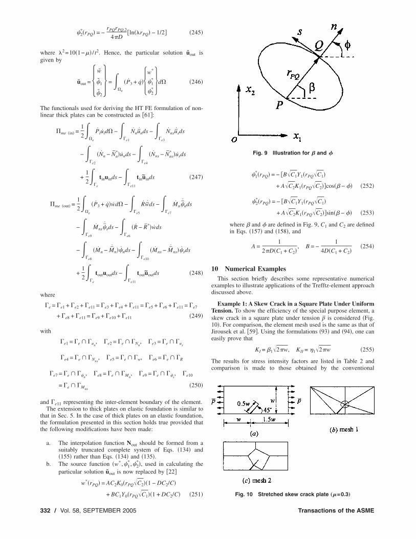
�2*�rPQ� = −

rPQrPQ,2

4�D�ln��rPQ� − 1/2� �245�

where �2=10�1−�� / t2. Hence, the particular solution uout isgiven by

uout = � w

�1

�2

� = �e

�P3 + q��w*

�1*

�2* �d� �246�

The functionals used for deriving the HT FE formulation of non-linear thick plates can be constructed as �61�:

me �in� =1

2 �e

Piuid� − �e1

Nnunds − �e3

Nnsusds

− �e2

�Nn − Nn*�unds −

�e4

�Nns − Nns* �usds

+1

2 �e

tinuinds − �e11

tinuinds �247�

me �out� =1

2 �e

�P3 + q�wd� − �e5

Rwds − �e7

Mn�˙

nds

− �e9

Mns�˙

sds − �e6

�R − R*�wds

− �e8

�Mn − M˙

n��nds − �e10

�Mns − M˙

ns��sds

+1

2 �e

toutuoutds − �e11

toutuoutds �248�

where

�e = �e1 + �e2 + �e11 = �e3 + �e4 + �e11 = �e5 + �e6 + �e11 = �e7

+ �e8 + �e11 = �e9 + �e10 + �e11 �249�

with

�e1 = �e � �un, �e2 = �e � �Nn

, �e3 = �e � �us

�e4 = �e � �Nns, �e5 = �e � �w, �e6 = �e � �R

�e7 = �e � ��n, �e8 = �e � �Mn

, �e9 = �e � ��s, �e10

= �e � �Mns�250�

and �e11 representing the inter-element boundary of the element.The extension to thick plates on elastic foundation is similar to

that in Sec. 5. In the case of thick plates on an elastic foundation,the formulation presented in this section holds true provided thatthe following modifications have been made:

a. The interpolation function Nout should be formed from asuitably truncated complete system of Eqs. �134� and�155� rather than Eqs. �134� and �135�.

b. The source function �w* ,�1* ,�2

*�, used in calculating theparticular solution uout is now replaced by �22�

w*�rPQ� = AC2K0�rPQ�C2��1 − DC2/C�

�
+ BC1Y0�rPQ C1��1 + DC2/C� �251�

�1*�rPQ� = − �B�C1Y1�rPQ

�C1�

+ A�C2K1�rPQ�C2��cos�� − �� 252�

�2*�rPQ� = − �B�C1Y1�rPQ

�C1�

+ A�C2K1�rPQ�C2��sin�� − �� 253�

where � and � are defined in Fig. 9, C1 and C2 are definedin Eqs. �157� and �158�, and

A =1

2�D�C1 + C2�, B = −

1

4D�C1 + C2��254�

10 Numerical ExamplesThis section briefly describes some representative numerical

examples to illustrate applications of the Trefftz-element approachdiscussed above.

Example 1: A Skew Crack in a Square Plate Under UniformTension. To show the efficiency of the special purpose element, askew crack in a square plate under tension p is considered �Fig.10�. For comparison, the element mesh used is the same as that ofJirousek et al. �59�. Using the formulations �93� and �94�, one caneasily prove that

KI = �1�2�w, KII = �1

�2�w �255�

The results for stress intensity factors are listed in Table 2 andcomparison is made to those obtained by the conventional

Fig. 9 Illustration for � and �

Fig. 10 Stretched skew crack plate „�=0.3…


p-element method �59�. It can be seen from Table 2 that the solu-tion from the HT p-element method may converge to a fixed valuerelatively quickly compared to the conventional p-elementmethod.

Example 2: Morley’s Skew Plate Problem (Fig. 11). The per-formance of a special-purpose corner element in singularity cal-culations is exemplified by analyzing the well-known Morley’sskew plate problem �Fig. 11�. For the skew plate angle of 30 deg,the plate exhibits a very strong singularity at the obtuse corners�the exponent of the leading singularity term Cr� of the deflectionexpansion is equal to 1.2�. Such a problem is considered difficultand has attracted the attention of research workers �29,148,149�.The difficulty is mainly attributable to the strong singularity at theobtuse corner, which causes most FE models either to convergevery slowly to the true solution or not to converge at all. Theanalytical solution of the problem based on the series expansionwith coefficients determined by the least-squares method was pre-sented by Morley �150�, whose results are generally used as

Table 2 Comparison of various predictions o10. Conventional results „mesh 1… taken=cutoff function method…. HT results „mesh 2…

KI / p�2�w

mConv. p elem.a

HT-pCIM CFM

0 0.54127 0.42259 0.465352 0.49708 0.55588 0.590124 0.58909 0.56161 0.599836 0.57864 0.59232 0.601428 0.60588 0.59825 0.6014910 0.59672 0.60043 0.6015112 0.60313 0.60119 —14 0.60032 0.60132 —

aData taken from �59�.

Fig. 11 Uniformly loaded simply supported 30 deg skew plate„L / t=100…

Fig. 12 Configuration of meshes used in finite elementanalysis

Table 3 Solution with special purpose cornMorley’s simply supported uniformly loaded s

Mesh quantity M =

2�2 wc −6.0M11c −5.0M22c −27.8

3�3 wc −1.9M11c

0.92M22c

3.254�4 wc −1.5

M11c0.39

M22c2.25


reference.The numerical results for different meshes �2�2, 3�3, 4�4,

shown in Fig. 12� are obtained at the plate center and displayed inTables 3 and 4, and are compared to Morley’s results �wc=0.000408qL4 /D, M11c=0.0108qL2 and M22c=0.0191qL2�. In thecalculation, 10 corner functions have been used.

The high efficiency of special-purpose corner functions for thesolution of singularity problems can be seen from Tables 3 and 4.Such functions play an even more important role within theT-element model where, by definition, the expansion basis of eachelement is optional. This feature enables involved singularity orstress concentration problems to be efficiently solved withouttroublesome mesh refinement. It is also evident from Tables 3 and4 that the Trefftz-element model performs well with regard to pconvergence, i.e., the numerical results converge quickly to theanalytical results along with increase of M.

Example 3: Large Deflection for an Annular Plate on aPasternak-Type Foundation. The annular plate is subjected to auniform distributed load q �Q=qa4 /Et4� and rests on a Pasternak-type foundation. The inner boundary of the plate is in a free-edgecondition, whereas the outer boundary condition is clamped im-movable. Some initial data used in the example are given by

GPa2/Et3 = 1, K = kPa4/Et3 = 5, b/a = 1/3, � = 1/3

where a and b are the outer and inner radii of the annular plate�Fig. 13�. In the example, a quarter of the plate is modeled by thethree meshes shown in Fig. 13. The loading step is taken as �Q=5. Some results obtained by the proposed method are listed inTables 5 and 6.

11 Conclusions and Future DevelopmentsOn the basis of the preceding discussion, the following conclu-

sions can be drawn. In contrast to conventional FE and boundary

I and KII for the skew crack problem from Fig.m †59‡ „CIM=contour integral method, CFMtained from Eq. „255….

KII / p�2�wConv. p elem.a

HT-pCIM CFM

−0.37480 −0.29005 −0.28433−0.25578 −0.28292 −0.28669−0.28951 −0.27474 −0.29067−0.28319 −0.29022 −0.29092−0.29398 −0.29012 −0.29095−0.28997 −0.29097 −0.29096−0.29196 −0.29091 —−0.29042 −0.29095 —

functions applied to all corner elements for30 deg plate

Percentage error3 5 7

0.55 0.0 0.03.32 1.08 0.015.44 0.97 0.030.31 0.0 0.00.27 0.0 0.01.02 0.03 0.00.01 0.0 0.00.11 0.0 0.00.98 0.01 0.0

f Kfroob

erkew

1

836

8

8


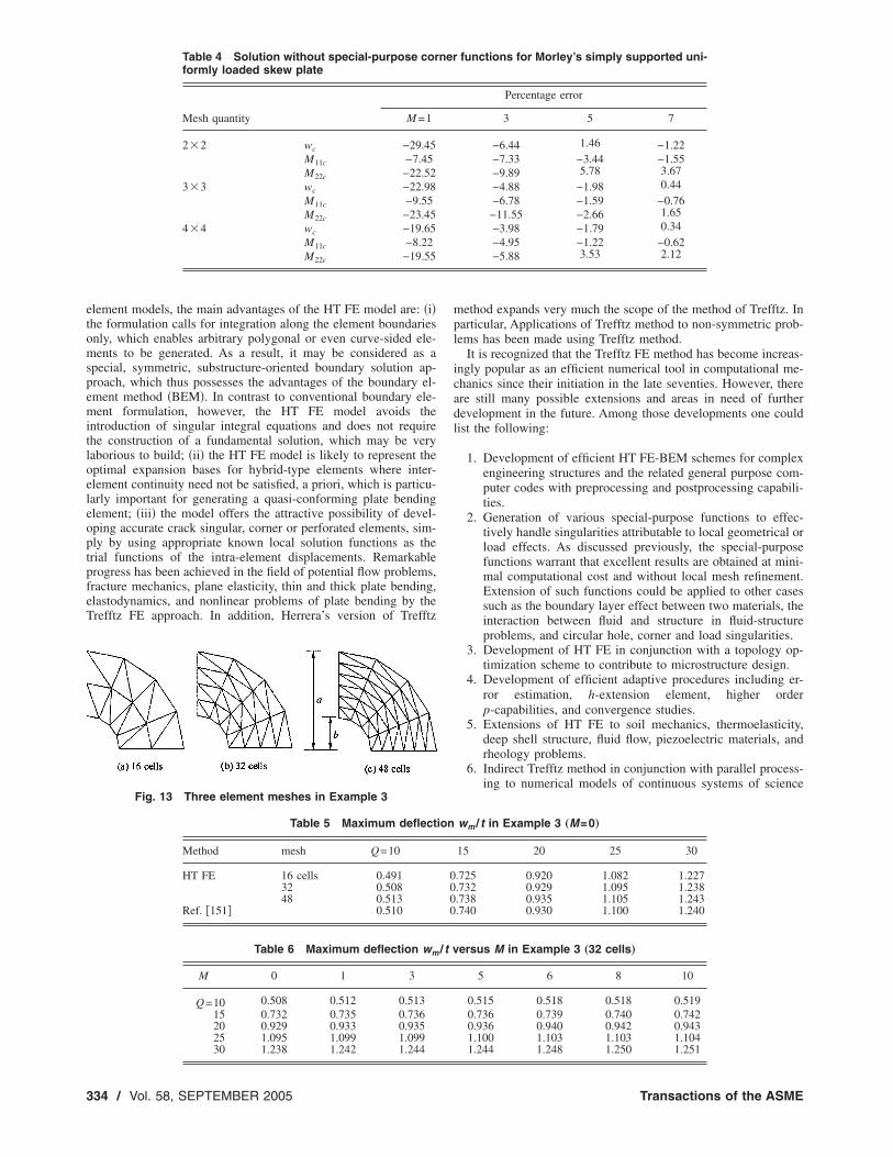
element models, the main advantages of the HT FE model are: �i�the formulation calls for integration along the element boundariesonly, which enables arbitrary polygonal or even curve-sided ele-ments to be generated. As a result, it may be considered as aspecial, symmetric, substructure-oriented boundary solution ap-proach, which thus possesses the advantages of the boundary el-ement method �BEM�. In contrast to conventional boundary ele-ment formulation, however, the HT FE model avoids theintroduction of singular integral equations and does not requirethe construction of a fundamental solution, which may be verylaborious to build; �ii� the HT FE model is likely to represent theoptimal expansion bases for hybrid-type elements where inter-element continuity need not be satisfied, a priori, which is particu-larly important for generating a quasi-conforming plate bendingelement; �iii� the model offers the attractive possibility of devel-oping accurate crack singular, corner or perforated elements, sim-ply by using appropriate known local solution functions as thetrial functions of the intra-element displacements. Remarkableprogress has been achieved in the field of potential flow problems,fracture mechanics, plane elasticity, thin and thick plate bending,elastodynamics, and nonlinear problems of plate bending by theTrefftz FE approach. In addition, Herrera’s version of Trefftz

Table 4 Solution without special-purpose corformly loaded skew plate

Mesh quantity M =1

2�2 wc −29.45M11c −7.45M22c −22.52

3�3 wc −22.98M11c −9.55M22c −23.45

4�4 wc −19.65M11c −8.22M22c −19.55

Fig. 13 Three element meshes in Example 3

Table 5 Maximum deflect

Method mesh Q=10

HT FE 16 cells 0.49132 0.50848 0.513

Ref. �151� 0.510

Table 6 Maximum deflection wm

M 0 1 3

Q=10 0.508 0.512 0.51315 0.732 0.735 0.73620 0.929 0.933 0.93525 1.095 1.099 1.09930 1.238 1.242 1.244


method expands very much the scope of the method of Trefftz. Inparticular, Applications of Trefftz method to non-symmetric prob-lems has been made using Trefftz method.

It is recognized that the Trefftz FE method has become increas-ingly popular as an efficient numerical tool in computational me-chanics since their initiation in the late seventies. However, thereare still many possible extensions and areas in need of furtherdevelopment in the future. Among those developments one couldlist the following:

1. Development of efficient HT FE-BEM schemes for complexengineering structures and the related general purpose com-puter codes with preprocessing and postprocessing capabili-ties.

2. Generation of various special-purpose functions to effec-tively handle singularities attributable to local geometrical orload effects. As discussed previously, the special-purposefunctions warrant that excellent results are obtained at mini-mal computational cost and without local mesh refinement.Extension of such functions could be applied to other casessuch as the boundary layer effect between two materials, theinteraction between fluid and structure in fluid-structureproblems, and circular hole, corner and load singularities.

3. Development of HT FE in conjunction with a topology op-timization scheme to contribute to microstructure design.

4. Development of efficient adaptive procedures including er-ror estimation, h-extension element, higher orderp-capabilities, and convergence studies.

5. Extensions of HT FE to soil mechanics, thermoelasticity,deep shell structure, fluid flow, piezoelectric materials, andrheology problems.

6. Indirect Trefftz method in conjunction with parallel process-ing to numerical models of continuous systems of science

functions for Morley’s simply supported uni-

Percentage error

3 5 7

−6.44 1.46 −1.22−7.33 −3.44 −1.55−9.89 5.78 3.67−4.88 −1.98 0.44−6.78 −1.59 −0.76−11.55 −2.66 1.65−3.98 −1.79 0.34−4.95 −1.22 −0.62−5.88 3.53 2.12

wm / t in Example 3 „M=0…

15 20 25 30

.725 0.920 1.082 1.227

.732 0.929 1.095 1.238

.738 0.935 1.105 1.243

.740 0.930 1.100 1.240

ersus M in Example 3 „32 cells…

5 6 8 10

0.515 0.518 0.518 0.5190.736 0.739 0.740 0.7420.936 0.940 0.942 0.9431.100 1.103 1.103 1.1041.244 1.248 1.250 1.251

ner

ion

0000

/ t v


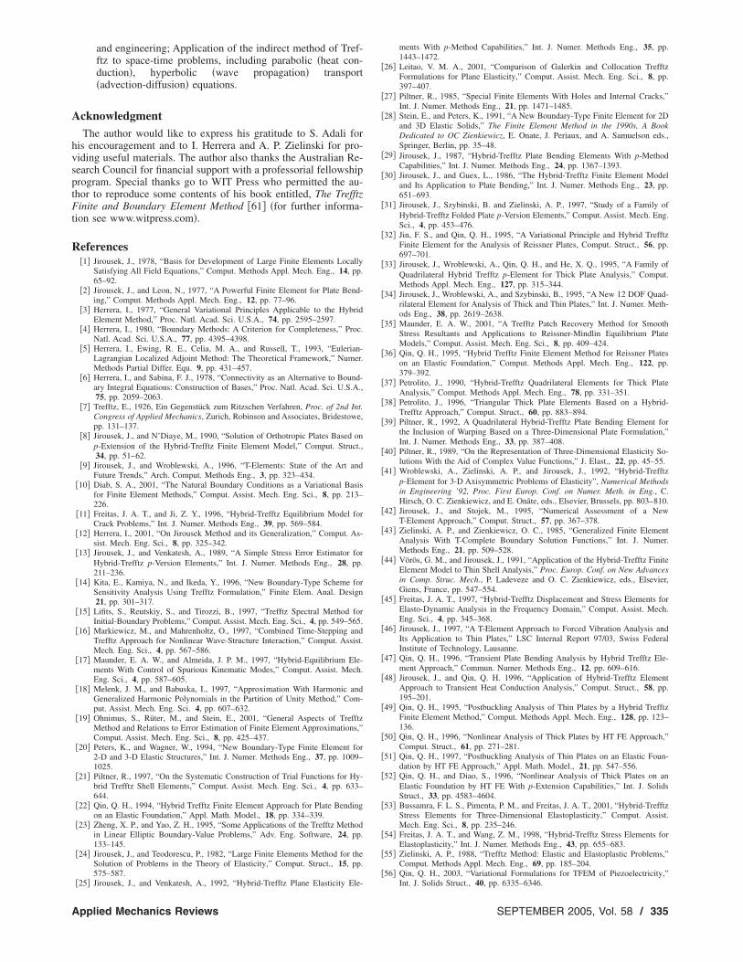
and engineering; Application of the indirect method of Tref-ftz to space-time problems, including parabolic �heat con-duction�, hyperbolic �wave propagation� transport�advection-diffusion� equations.

AcknowledgmentThe author would like to express his gratitude to S. Adali for

his encouragement and to I. Herrera and A. P. Zielinski for pro-viding useful materials. The author also thanks the Australian Re-search Council for financial support with a professorial fellowshipprogram. Special thanks go to WIT Press who permitted the au-thor to reproduce some contents of his book entitled, The TrefftzFinite and Boundary Element Method �61� �for further informa-tion see www.witpress.com�.

References�1� Jirousek, J., 1978, “Basis for Development of Large Finite Elements Locally

Satisfying All Field Equations,” Comput. Methods Appl. Mech. Eng., 14, pp.65–92.

�2� Jirousek, J., and Leon, N., 1977, “A Powerful Finite Element for Plate Bend-ing,” Comput. Methods Appl. Mech. Eng., 12, pp. 77–96.

�3� Herrera, I., 1977, “General Variational Principles Applicable to the HybridElement Method,” Proc. Natl. Acad. Sci. U.S.A., 74, pp. 2595–2597.

�4� Herrera, I., 1980, “Boundary Methods: A Criterion for Completeness,” Proc.Natl. Acad. Sci. U.S.A., 77, pp. 4395–4398.

�5� Herrera, I., Ewing, R. E., Celia, M. A., and Russell, T., 1993, “Eulerian-Lagrangian Localized Adjoint Method: The Theoretical Framework,” Numer.Methods Partial Differ. Equ. 9, pp. 431–457.

�6� Herrera, I., and Sabina, F. J., 1978, “Connectivity as an Alternative to Bound-ary Integral Equations: Construction of Bases,” Proc. Natl. Acad. Sci. U.S.A.,75, pp. 2059–2063.

�7� Trefftz, E., 1926, Ein Gegenstück zum Ritzschen Verfahren, Proc. of 2nd Int.Congress of Applied Mechanics, Zurich, Robinson and Associates, Bridestowe,pp. 131–137.

�8� Jirousek, J., and N’Diaye, M., 1990, “Solution of Orthotropic Plates Based onp-Extension of the Hybrid-Trefftz Finite Element Model,” Comput. Struct.,34, pp. 51–62.

�9� Jirousek, J., and Wroblewski, A., 1996, “T-Elements: State of the Art andFuture Trends,” Arch. Comput. Methods Eng., 3, pp. 323–434.

�10� Diab, S. A., 2001, “The Natural Boundary Conditions as a Variational Basisfor Finite Element Methods,” Comput. Assist. Mech. Eng. Sci., 8, pp. 213–226.

�11� Freitas, J. A. T., and Ji, Z. Y., 1996, “Hybrid-Trefftz Equilibrium Model forCrack Problems,” Int. J. Numer. Methods Eng., 39, pp. 569–584.

�12� Herrera, I., 2001, “On Jirousek Method and its Generalization,” Comput. As-sist. Mech. Eng. Sci., 8, pp. 325–342.

�13� Jirousek, J., and Venkatesh, A., 1989, “A Simple Stress Error Estimator forHybrid-Trefftz p-Version Elements,” Int. J. Numer. Methods Eng., 28, pp.211–236.

�14� Kita, E., Kamiya, N., and Ikeda, Y., 1996, “New Boundary-Type Scheme forSensitivity Analysis Using Trefftz Formulation,” Finite Elem. Anal. Design21, pp. 301–317.

�15� Lifits, S., Reutskiy, S., and Tirozzi, B., 1997, “Trefftz Spectral Method forInitial-Boundary Problems,” Comput. Assist. Mech. Eng. Sci., 4, pp. 549–565.

�16� Markiewicz, M., and Mahrenholtz, O., 1997, “Combined Time-Stepping andTrefftz Approach for Nonlinear Wave-Structure Interaction,” Comput. Assist.Mech. Eng. Sci., 4, pp. 567–586.

�17� Maunder, E. A. W., and Almeida, J. P. M., 1997, “Hybrid-Equilibrium Ele-ments With Control of Spurious Kinematic Modes,” Comput. Assist. Mech.Eng. Sci., 4, pp. 587–605.

�18� Melenk, J. M., and Babuska, I., 1997, “Approximation With Harmonic andGeneralized Harmonic Polynomials in the Partition of Unity Method,” Com-put. Assist. Mech. Eng. Sci. 4, pp. 607–632.

�19� Ohnimus, S., Rüter, M., and Stein, E., 2001, “General Aspects of TrefftzMethod and Relations to Error Estimation of Finite Element Approximations,”Comput. Assist. Mech. Eng. Sci., 8, pp. 425–437.

�20� Peters, K., and Wagner, W., 1994, “New Boundary-Type Finite Element for2-D and 3-D Elastic Structures,” Int. J. Numer. Methods Eng., 37, pp. 1009–1025.

�21� Piltner, R., 1997, “On the Systematic Construction of Trial Functions for Hy-brid Trefftz Shell Elements,” Comput. Assist. Mech. Eng. Sci., 4, pp. 633–644.

�22� Qin, Q. H., 1994, “Hybrid Trefftz Finite Element Approach for Plate Bendingon an Elastic Foundation,” Appl. Math. Model., 18, pp. 334–339.

�23� Zheng, X. P., and Yao, Z. H., 1995, “Some Applications of the Trefftz Methodin Linear Elliptic Boundary-Value Problems,” Adv. Eng. Software, 24, pp.133–145.

�24� Jirousek, J., and Teodorescu, P., 1982, “Large Finite Elements Method for theSolution of Problems in the Theory of Elasticity,” Comput. Struct., 15, pp.575–587.

�25� Jirousek, J., and Venkatesh, A., 1992, “Hybrid-Trefftz Plane Elasticity Ele-


ments With p-Method Capabilities,” Int. J. Numer. Methods Eng., 35, pp.1443–1472.

�26� Leitao, V. M. A., 2001, “Comparison of Galerkin and Collocation TrefftzFormulations for Plane Elasticity,” Comput. Assist. Mech. Eng. Sci., 8, pp.397–407.

�27� Piltner, R., 1985, “Special Finite Elements With Holes and Internal Cracks,”Int. J. Numer. Methods Eng., 21, pp. 1471–1485.

�28� Stein, E., and Peters, K., 1991, “A New Boundary-Type Finite Element for 2Dand 3D Elastic Solids,” The Finite Element Method in the 1990s, A BookDedicated to OC Zienkiewicz, E. Onate, J. Periaux, and A. Samuelson eds.,Springer, Berlin, pp. 35–48.

�29� Jirousek, J., 1987, “Hybrid-Trefftz Plate Bending Elements With p-MethodCapabilities,” Int. J. Numer. Methods Eng., 24, pp. 1367–1393.

�30� Jirousek, J., and Guex, L., 1986, “The Hybrid-Trefftz Finite Element Modeland Its Application to Plate Bending,” Int. J. Numer. Methods Eng., 23, pp.651–693.

�31� Jirousek, J., Szybinski, B. and Zielinski, A. P., 1997, “Study of a Family ofHybrid-Trefftz Folded Plate p-Version Elements,” Comput. Assist. Mech. Eng.Sci., 4, pp. 453–476.

�32� Jin, F. S., and Qin, Q. H., 1995, “A Variational Principle and Hybrid TrefftzFinite Element for the Analysis of Reissner Plates, Comput. Struct., 56, pp.697–701.

�33� Jirousek, J., Wroblewski, A., Qin, Q. H., and He, X. Q., 1995, “A Family ofQuadrilateral Hybrid Trefftz p-Element for Thick Plate Analysis,” Comput.Methods Appl. Mech. Eng., 127, pp. 315–344.

�34� Jirousek, J., Wroblewski, A., and Szybinski, B., 1995, “A New 12 DOF Quad-rilateral Element for Analysis of Thick and Thin Plates,” Int. J. Numer. Meth-ods Eng., 38, pp. 2619–2638.

�35� Maunder, E. A. W., 2001, “A Trefftz Patch Recovery Method for SmoothStress Resultants and Applications to Reissner-Mindlin Equilibrium PlateModels,” Comput. Assist. Mech. Eng. Sci., 8, pp. 409–424.

�36� Qin, Q. H., 1995, “Hybrid Trefftz Finite Element Method for Reissner Plateson an Elastic Foundation,” Comput. Methods Appl. Mech. Eng., 122, pp.379–392.

�37� Petrolito, J., 1990, “Hybrid-Trefftz Quadrilateral Elements for Thick PlateAnalysis,” Comput. Methods Appl. Mech. Eng., 78, pp. 331–351.

�38� Petrolito, J., 1996, “Triangular Thick Plate Elements Based on a Hybrid-Trefftz Approach,” Comput. Struct., 60, pp. 883–894.

�39� Piltner, R., 1992, A Quadrilateral Hybrid-Trefftz Plate Bending Element forthe Inclusion of Warping Based on a Three-Dimensional Plate Formulation,”Int. J. Numer. Methods Eng., 33, pp. 387–408.

�40� Piltner, R., 1989, “On the Representation of Three-Dimensional Elasticity So-lutions With the Aid of Complex Value Functions,” J. Elast., 22, pp. 45–55.

�41� Wroblewski, A., Zielinski, A. P., and Jirousek, J., 1992, “Hybrid-Trefftzp-Element for 3-D Axisymmetric Problems of Elasticity”, Numerical Methodsin Engineering ’92, Proc. First Europ. Conf. on Numer. Meth. in Eng., C.Hirsch, O. C. Zienkiewicz, and E. Onãte, eds., Elsevier, Brussels, pp. 803–810.

�42� Jirousek, J., and Stojek, M., 1995, “Numerical Assessment of a NewT-Element Approach,” Comput. Struct., 57, pp. 367–378.

�43� Zielinski, A. P., and Zienkiewicz, O. C., 1985, “Generalized Finite ElementAnalysis With T-Complete Boundary Solution Functions,” Int. J. Numer.Methods Eng., 21, pp. 509–528.

�44� Vörös, G. M., and Jirousek, J., 1991, “Application of the Hybrid-Trefftz FiniteElement Model to Thin Shell Analysis,” Proc. Europ. Conf. on New Advancesin Comp. Struc. Mech., P. Ladeveze and O. C. Zienkiewicz, eds., Elsevier,Giens, France, pp. 547–554.

�45� Freitas, J. A. T., 1997, “Hybrid-Trefftz Displacement and Stress Elements forElasto-Dynamic Analysis in the Frequency Domain,” Comput. Assist. Mech.Eng. Sci., 4, pp. 345–368.

�46� Jirousek, J., 1997, “A T-Element Approach to Forced Vibration Analysis andIts Application to Thin Plates,” LSC Internal Report 97/03, Swiss FederalInstitute of Technology, Lausanne.

�47� Qin, Q. H., 1996, “Transient Plate Bending Analysis by Hybrid Trefftz Ele-ment Approach,” Commun. Numer. Methods Eng., 12, pp. 609–616.

�48� Jirousek, J., and Qin, Q. H. 1996, “Application of Hybrid-Trefftz ElementApproach to Transient Heat Conduction Analysis,” Comput. Struct., 58, pp.195–201.

�49� Qin, Q. H., 1995, “Postbuckling Analysis of Thin Plates by a Hybrid TrefftzFinite Element Method,” Comput. Methods Appl. Mech. Eng., 128, pp. 123–136.

�50� Qin, Q. H., 1996, “Nonlinear Analysis of Thick Plates by HT FE Approach,”Comput. Struct., 61, pp. 271–281.

�51� Qin, Q. H., 1997, “Postbuckling Analysis of Thin Plates on an Elastic Foun-dation by HT FE Approach,” Appl. Math. Model., 21, pp. 547–556.

�52� Qin, Q. H., and Diao, S., 1996, “Nonlinear Analysis of Thick Plates on anElastic Foundation by HT FE With p-Extension Capabilities,” Int. J. SolidsStruct., 33, pp. 4583–4604.

�53� Bussamra, F. L. S., Pimenta, P. M., and Freitas, J. A. T., 2001, “Hybrid-TrefftzStress Elements for Three-Dimensional Elastoplasticity,” Comput. Assist.Mech. Eng. Sci., 8, pp. 235–246.

�54� Freitas, J. A. T., and Wang, Z. M., 1998, “Hybrid-Trefftz Stress Elements forElastoplasticity,” Int. J. Numer. Methods Eng., 43, pp. 655–683.

�55� Zielinski, A. P., 1988, “Trefftz Method: Elastic and Elastoplastic Problems,”Comput. Methods Appl. Mech. Eng., 69, pp. 185–204.

�56� Qin, Q. H., 2003, “Variational Formulations for TFEM of Piezoelectricity,”
Int. J. Solids Struct., 40, pp. 6335–6346.

�57� Qin, Q. H., 2003, “Solving Anti-Plane Problems of Piezoelectric Materials bythe Trefftz Finite Element Approach,” Comput. Mech., 31, pp. 461–468.

�58� Venkatesh, A., and Jirousek, J., 1995, “Accurate Representation of Local Ef-fect Due to Concentrated and Discontinuous Loads in Hybrid-Trefftz PlateBending Elements,” Comput. Struct., 57, pp. 863–870.

�59� Jirousek, J., Venkatesh, A., Zielinski, A. P., and Rabemanantsoo, H., 1993,“Comparative Study of p-Extensions Based on Conventional Assumed Dis-placement and Hybrid-Trefftz FE Models,” Comput. Struct., 46, pp. 261–278.

�60� Huang, H. T., and Li, Z. C., 2003, “Global Superconvergence of Adini’s Ele-ments Coupled With Trefftz Method for Singular Problems,” Eng. Anal.Boundary Elem., 27, pp. 227–240.

�61� Qin, Q. H., 2000, The Trefftz Finite and Boundary Element Method, WITPress, Southampton.

�62� Herrera, I., 1997, “Trefftz-Herrera Method,” Comput. Assist. Mech. Eng. Sci.,4, pp. 369–382.

�63� Jirousek, J., 1991, “New Trends in HT-p Element Approach,” The Finite Ele-ment Method in the 1990s, E. Onate, J. Periaux, and A. Samuelson, eds.,Springer, Berlin.

�64� Jirousek, J., and Wroblewski, A., 1995, “T-Elements: A Finite Element Ap-proach With Advantages of Boundary Solution Methods, Adv. Eng. Software24, 71-88.

�65� Jirousek, J., and Zieliński, A. P., 1997, “Survey of Trefftz-Type Element For-mulations,” Comput. Struct., 63, pp. 225–242.

�66� Kita, E., and Kamiya, N., 1995, “Trefftz Method: An Overview,” Adv. Eng.Software, 24, pp. 3–12.

�67� Qin, Q. H., 1993, “A Brief Introduction and Prospect to Hybrid-Trefftz FiniteElements,” Mech. Pract., 15, pp. 20–22 �in Chinese�.

�68� Qin, Q. H., 1998, “The Study and Prospect of Hybrid-Trefftz Finite ElementMethod,” Adv. Mech., 28, pp. 71–80 �in Chinese�.

�69� Zienkiewicz, O. C., 1997, “Trefftz Type Approximation and the GeneralisedFinite Element Method: History and Development,” Comput. Assist. Mech.Eng. Sci., 4, pp. 305–316.

�70� Gourgeon, H., and Herrera, I., 1981, “Boundary Methods: C-Complete Sys-tems for Biharmonic Equations,” Boundary Element Methods, C. A. Brebbia,ed., pp. 431–441, Springer-Verlag, Berlin.

�71� Herrera, I., 1977, “Theory of Connectivity Formal Symmetric Operators,”Proc. Natl. Acad. Sci. U.S.A., 74, pp. 4722–4725.

�72� Celia, M., and Herrera, I., 1987, “Solution of General Differential EquationsUsing the Algebraic Theory Approach,” Numer. Methods Partial Differ. Equ.,3, pp. 117–129.

�73� Herrera, I., 1987, “The Algebraic Theory Approach for Ordinary DifferentialEquations: Highly Accurate Finite Differences,” Numer. Methods Partial Dif-fer. Equ., 3, pp. 199–218.

�74� Herrera, I., 1992, “Localized Adjoint Methods: A New Discretization Method-ology,” Computational Methods in Geosciences, W. E. Fitzgibbon and M. F.Wheeler, eds., SIAM, Philadelphia, Chap. 6, pp. 66–77.

�75� Herrera, I., 2000, “Trefftz Method: A General Theory,” Numer. Methods Par-tial Differ. Equ., 16, pp. 561–580.

�76� Herrera, I., 2002, “The Indirect Approach to Domain Decomposition,” 14thInt. Conf. on Domain Decomposition Methods, Cocoyoc, Mor., Mex., InvitedPlenary Lecture, www.ddm.org

�77� Herrera, I. 2002, “A Unified Theory of Domain Decomposition Methods,”14th Int. Conf. on Domain Decomposition Methods, Cocoyoc, Mor., Mex.,www.ddm.org

�78� Herrera, I., and Yates, R., 2001, “General Theory of Domain Decomposition:Beyond Schwarz Methods,” Numer. Methods Partial Differ. Equ., 17, pp.495–517.

�79� Herrera, I., Yates, R., and Diaz, M., 2002, “General Theory of Domain De-composition: Indirect Methods,” Numer. Methods Partial Differ. Equ., 18, pp.296–322.

�80� Díaz, M., Herrera, I., and Yates, R., 2002, “Indirect Method of Collocation,”14th Int. Conf. on Domain Decomposition Methods, Cocoyoc, Mor., Mex.,www.ddm.org

�81� Yates, R., and Herrera, I., 2002, “Parallel Implementation of Indirect Colloca-tion Methods,” 14th Int. Conf. on Domain Decomposition Methods, Cocoyoc,Mor., Mex. www.ddm.org

�82� Herrera, I., 1985, “Unified Approach to Numerical Methods. I. Green’s For-mulas for Operators in Discontinuous Fields,” Numer. Methods Partial Differ.Equ., 1, pp. 12–37.

�83� Herrera, I., Chargoy, L., and Alduncin, G., 1985, “Unified Approach to Nu-merical Methods. Part 3. Finite Differences and Ordinary Differential Equa-tions,” Numer. Methods Partial Differ. Equ., 1, pp. 241–258.

�84� Jirousek, J., 1993, “Variational Formulation of Two Complementary Hybrid-Trefftz FE Models,” Commun. Numer. Methods Eng., 9, pp. 837–845.

�85� Jirousek, J., and Zielinski, A. P., 1993, “Dual Hybrid-Trefftz Element Formu-lation Based on Independent Boundary Traction Frame,” Int. J. Numer. Meth-ods Eng., 36, pp. 2955–2980.

�86� Cheung, Y. K., Jin, W. G., and Zienkiewicz, O. C., 1989, “Direct SolutionProcedure for Solution of Harmonic Problems Using Complete, Non-Singular,Trefftz Functions,” Commun. Appl. Numer. Methods, 5, pp. 159–169.

�87� Cheung, Y. K., Jin, W. G., and Zienkiewicz, O. C., 1991, “Solution of Helm-holtz Equation by Trefftz Method,” Int. J. Numer. Methods Eng., 32, pp.63–78.

�88� Jirousek, J., and Wroblewski, A., 1994, “Least-Squares T-Elements: Equiva-lent FE and BE Forms of a Substructure-Oriented Boundary Solution Ap-proach,” Commun. Numer. Methods Eng., 10, pp. 21–32.

�89� Stojek, M., 1998, “Least-Squares Trefftz-Type Elements for the Helmholtz


Equation,” Int. J. Numer. Methods Eng., 41, pp. 831–849.�90� Cialkowski, M. J., 2001, “Trefftz Functions as Basic Functions of FEM in

Application to Solution of Inverse Heat Conduction Problem,” Comput. Assist.Mech. Eng. Sci., 8, pp. 247–260.

�91� Desmet, W., Sas, P., and Vandepitte, D., 2001, “An Indirect Trefftz Method forthe Steady-State Dynamic Analysis of Coupled Vibro-Acoustic Systems,”Comput. Assist. Mech. Eng. Sci., 8, pp. 271–288.

�92� Hsiao, G. C., Schnack, E., and Wendland, W. L., 2000, “Hybrid CoupledFinite-Boundary Element Methods for Elliptic Systems of Second Order,”Comput. Methods Appl. Mech. Eng., 190, pp. 431–485.

�93� Ihlenburg, F., and Babuska, I., 1997, “Solution of Helmholtz Problems byKnowledge-Based FEM,” Comput. Assist. Mech. Eng. Sci., 4, pp. 397–415.

�94� Kita, E., Kamiya, N., and Ikeda, Y., 1997, “First- and Second-Order SensitivityAnalysis Schemes by Collocation-Type Trefftz Method,” Comput. Assist.Mech. Eng. Sci., 4, pp. 477–489.

�95� Kolodziej, J. A., and Mendes, A. C., 2001, “T-Functions for 2-D CreepingFlow on Domains With Circular Cylinders, Corners, and Processing Symme-try,” Comput. Assist. Mech. Eng. Sci., 8, pp. 359–384.

�96� Kolodziej, J. A., and Uscilowska, A., 1997, “Trefftz-Type Procedure forLaplace Equation on Domains With Circular Holes, Circular Inclusions, Cor-ners, Slits, and Symmetry,” Comput. Assist. Mech. Eng. Sci. 4, pp. 501–519.

�97� Stojek, M., Markiewicz, M., and Mahrenholtz, O., 2000, “Diffraction Loads onMultiple Vertical Cylinders With Rectangular Cross Section by Trefftz-TypeFinite Elements,” Comput. Struct., 75, pp. 335–345.

�98� Zielinski, A. P., 1997, “Special Trefftz Elements and Improvement of TheirConditioning,” Commun. Numer. Methods Eng., 13, pp. 765–775.

�99� Freitas, J. A. T., and Bussamra, F. L. S., 2000, “Three-Dimensional Hybrid-Trefftz Stress Elements,” Int. J. Numer. Methods Eng., 47, pp. 927–950.

�100� Freitas, J. A. T., and Cismasiu, I., 2002, “Shape Optimizing With Hybrid-Trefftz Displacement Elements,” Int. J. Numer. Methods Eng., 53, pp. 473–498.

�101� Hsiao, G. C., Schnack, E., and Wendland, W. L., 1999, “A Hybrid CoupledFinite-Boundary Element Method in Elasticity,” Comput. Methods Appl.Mech. Eng., 173, pp. 287–316.

�102� Jin, W. G., Cheung, Y. K., and Zienkiewicz, O. C., 1990, “Application ofTrefftz Method in Plane Elasticity,” Int. J. Numer. Methods Eng., 30, pp.1147–1161.

�103� Qin, Q. H., 2004, “Dual Variational Formulation for Trefftz Finite ElementMethod of Elastic Materials,” Mech. Res. Commun., 31, pp. 321–330.

�104� Kompis, V., Konkol, F., and Vasko, M., 2001, “Trefftz-Polynomial Reciproc-ity Based FE Formulations,” Comput. Assist. Mech. Eng. Sci., 8, pp. 385–395.

�105� Kompis, V., Pavol, N., and Mariam, H., 2002, “Finite Displacements inReciprocity-Based FE Formulation,” Comput. Assist. Mech. Eng. Sci., 9, pp.469–480.

�106� Sladek, J., and Sladek, V., 2002, “A Trefftz Function Approximation in LocalBoundary Integral Equations,” Comput. Mech., 28, pp. 212–219.

�107� Sladek, J., Sladek, V., Kompis, V., and Van Keer, R., 2000, “Application ofMulti-Region Trefftz Method to Elasticity,” Comput. Model. Eng. Sci., 1,pp. 1–8.

�108� Jin, W. G., Cheung, Y. K., and Zienkiewicz, O. C., 1993, “Trefftz Method forKirchhoff Plate Bending Problems,” Int. J. Numer. Methods Eng., 36, pp.765–781.

�109� Jirousek, J., Zieliński, A. P., and Wróblewski, A. 2001, “T-Element Analysisof Plates on Unilateral Elastic Winkler-Type Foundation,” Computer AssistedMech. Eng. Sci., 8, pp. 343–358.

�110� Venkatesh, A. and Jirousek, J., 1987, “An Improved 9 DOF Hybrid-TrefftzTriangular Element for Plate Bending,” Eng. Comput., 4, pp. 207–222.

�111� Brink, U., Kkreienmeyer, M., Peters, K., and Stein, E., 1997, “Aspects ofTrefftz Method in BEM and FEM and Their Coupling,” Comput. Assist.Mech. Eng. Sci., 4, pp. 327–344.

�112� Chang, J. R., Liu, R. F., Yeih, W. C., and Kuo, S. R., 2002, “Applications ofthe Direct Trefftz Boundary Element Method to the Free-Vibration Problemof a Membrane,” J. Acoust. Soc. Am., 112, pp. 518–527.

�113� Freitas, J. A. T., 2002, “Mixed Finite Element Formulation for the Solution ofParabolic Problems,” Comput. Methods Appl. Mech. Eng., 191, pp. 3425–3457.

�114� Gyimesi, M., Wang, J. S., and Ostergaard, D., 2001, “Hybrid p-Element andTrefftz Method for Capacitance Computation,” IEEE Trans. Magn., 37, pp.3680–3683.

�115� He, J. H., 2002, “Generalized Variational Principles for Thermopiezoelectric-ity,” Arch. Appl. Mech., 72, pp. 248–256.

�116� Jirousek, J., and Venkatesh, A., 1990, “A New FE Approach for AdaptiveReliability Assurance,” Comput. Struct., 37, pp. 217–230.

�117� Karaś, M., and Zielinski, A. P., 2000, “Parametric Structural Shape Optimi-zation Using the Global Trefftz Approach,” Theor Appl. Mech., 38, pp. 285–296.

�118� Kompis, V., and Jakubovicova, L., 2000, “Errors in Modeling High OrderGradient Fields Using Reciprocity Based FEM,” Int. J. Eng. Model., 13, pp.27–34.

�119� Olegovich, Y., 2002, “Trefftz Finite Elements for Electromagnetics,” IEEETrans. Microwave Theory Tech., 50, pp. 1328–1339.

�120� Onuki, T., Wakao, S., Kuwahara, T., and Im, J. W., 1997, “Hybrid Trefftz andFinite Element Method Applied to Magnetic Field Analysis for Rotating Ma-chines,” IEEE Trans. Magn., 33, pp. 2014–2017.

�121� Reutskiy, S., 2002, “A Boundary Method of Trefftz Type With Approximate
Trial Functions,” Eng. Anal. Boundary Elem., 26, pp. 341–353.

�122� Szybiński, B., Wróblewski, A., Zieliński, A. P., 2001, “General Strategy ofh-p Adaptive Solutions in Structural Trefftz-Type Element Analysis,” Com-put. Assist. Mech. Eng. Sci., 8, pp. 469–477.

�123� Zieliński, A. P., and Herrera, I., 1987, “Trefftz Method: Fitting BoundaryConditions,” Int. J. Numer. Methods Eng., 24, pp. 871–891.

�124� Zieliński, A. P., Sanecki, H., and Karaś, M., 2001, “Effectiveness of theTrefftz Method in Different Engineering Optimization Procedures,” Comput.Assist. Mech. Eng. Sci., 8, pp. 479–493.

�125� Colton, D. L., 1976, Partial Differential Equations in the Complex Domain,Pitman, London.

�126� Henrici, P., 1960, “Complete Systems of Solutions for a Class of SingularElliptic Partial Differential Equations, Boundary problems in differentialequations, R. E. Langer, ed., University of Wisconsin Press, Madison.

�127� Herrera, I., 1984, Boundary Method: An Algebraic Theory, Pitman, Boston.�128� Sánchez, S. F. J., Herrera, I., and Avilés, J., 1982, A Boundary Method for

Elastic Wave Diffraction. Application to Scattering of SH-Waves by SurfaceIrregularities, Bull. Seismol. Soc. Am. 72, 473-490.

�129� Fung, Y. C., 1965, Foundations of Solid Mechanics, Prentice-Hall, Engle-wood Cliffs, NJ.

�130� Love, A. E. H., 1944, A Treatise on the Mathematical Theory of Elasticity,Dover, New York.

�131� Malvern, L. E., 1969, Introduction to the Mechanics of a Continuous Me-dium, Prentice-Hall, Englewood Cliffs, NJ.

�132� Muskhelishvili, N. I., 1953, Some Basic Problems of the MathematicalTheory of Elasticity, Noordhoff, Groningen, Holland.

�133� Sternberg, E., 1960, “On Some Recent Developments in the Linear Theory ofElasticity,” Proc. 1st Symp. on Naval Structural Mechanics, J. N. Goodierand N. J. Hoff, eds., Pergamon Press, New York.

�134� Williams, M. L., 1952, “Stress Singularities Resulting From Various Bound-ary Conditions in Angular Corners of Plates in Extension,” J. Appl. Mech.,19, pp. 526–528.

�135� Lin, K. Y., and Tong, P., 1980, “Singular Finite Elements for the FractureAnalysis of V-Notched Plate,” Int. J. Numer. Methods Eng., 15, pp. 1343–1354.

�136� Xu, Z., 1992, “A Thick-Thin Triangular Plate Element,” Int. J. Numer. Meth-ods Eng., 33, pp. 963–973.

�137� Aminpour, M. A., 1992, “Direct Formulation of a Hybrid 4-Node Shell Ele-


ment With Drilling Degrees of Freedom,” Int. J. Numer. Methods Eng., 35,pp. 997–1013.

�138� Ibrahimbergovic, A., 1993, “Quadrilateral Finite Elements for Analysis ofThick and Thin Plates,” Comput. Methods Appl. Mech. Eng., 110, pp. 195–209.

�139� Taylor, R. L., and Auricchio, F. A., 1993, “Linked Interpolation for Reissner-Mindlin Plate Elements. Part II. A Simple Triangle,” Int. J. Numer. MethodsEng., 36, pp. 3057–3066.

�140� Zienkiewicz, O. C., Xu, Z., Zeng, L. F., Samuelson, A., and Wiberg, N. E.,1993, “Linked Interpolation for Reissner-Mindlin Plate Elements. Part I. ASimple Quadrilateral,” Int. J. Numer. Methods Eng., 36, pp. 3043–3056.

�141� Mindlin, R. D., 1951, “Influence of Rotatory Inertia and Shear on FlexuralMotion of Isotropic Elastic Plates,” J. Appl. Mech., 18, pp. 31–38.

�142� Reissner, E., 1945, “The Effect of Shear Deformation on the Bending ofElastic Plates,” J. Appl. Mech., 12, pp. 69–76.

�143� Hu, H. C., 1963, “On Some Problems of the Antisymmetrical Small Deflec-tion of Isotropic Sandwich Plate,” Acta Mech. Sin. 6, pp. 53–60 �in Chi-nese�.

�144� Reismann, H., 1988, Elastic Plates: Theory and Applications, Wiley, NewYork.

�145� Qin, Q. H., 1998, “Nonlinear Analysis of Plate Bending by Boundary Ele-ment Method,” Plate Bending Analysis With Boundary Elements, M. H. Alia-badi, ed., Computational Mechanics Publications, Southampton, Chap. 8.

�146� Qin, Q. H., and Huang, Y. Y., 1990, “BEM of Postbuckling Analysis of ThinPlates,” Appl. Math. Model., 14, pp. 544–548.

�147� Qin, Q. H., 1993, “Nonlinear Analysis of Reissner Plates on an Elastic Foun-dation by the BEM,” Int. J. Solids Struct., 30, pp. 3101–3111.

�148� Argyris, J. H., and Lochner, N., 1972, “On the Application of SHEBA ShellElement,” Comput. Methods Appl. Mech. Eng., 1, pp. 317–347.

�149� Wang, D. W., Katz, I. N., and Szabo, B. A., 1984, “h- and p-Version FiniteElement Analysis of Rhombic Plate,” Int. J. Numer. Methods Eng., 20, pp.1399–1405.

�150� Morley, L. S. D., 1963, Skew Plates and Structures, Pergamon Press, Lon-don.

�151� Smaill, J. S., 1991, “Large Deflection Response of Annular Plates on Paster-nak Foundations,” Int. J. Solids Struct., 27, pp. 1073–1084.

Qing-Hua Qin received his Bachelor of Engineering degree in Mechanical Engineering from Xi’an High-way University (currently Chang An University), China in 1982, earning his Master of Science degree in1984 and Doctoral degree in 1990 from Huazhong University of Science and Technology (HUST) in China.Both degrees are in Applied Mechanics. He joined the Department of Mechanics as an Associate Lecturerat HUST in 1984, where he was until 1995. After spending ten years lecturing at HUST, he was awarded theDAAD/K.C. Wong research fellowship in 1994, which enabled him to work at the University of Stuttgart inGermany for nine months. In 1995 he left HUST to take up a postdoctoral fellowship at Tsinghua University,China. He was awarded a Queen Elizabeth II fellowship in 1997 and a professorial fellowship in 2002, bothby the Australian Research Council, and is currently working in the Department of Engineering at theAustralian National University, Australia. He has authored more than 100 published scientific papers andtwo books in the field of applied mechanics, and was a recipient of the J.G. Russell Award from theAustralian Academy of Science.


Trefftz Finite Element Method and Its Applications - Home - CECS - ANU

Documents

Transcript of Trefftz Finite Element Method and Its Applications - Home - CECS - ANU