Analysis of trace ﬁnite element methods for surface ...

IMA Journal of Numerical Analysis (2014) of 23doi:10.1093/imanum/dru047

Analysis of trace finite element methods for surface partial differential equations

Arnold Reusken

Institut für Geometrie und Praktische Mathematik, RWTH-Aachen University, D-52056 Aachen,Germany

∗Corresponding author: [email protected]

[Received on 19 March 2014; revised on 14 August 2014]

In this paper we consider two variants of a trace finite element method for solving elliptic partial differ-ential equations on a stationary smooth manifold Γ . A discretization error analysis for both methods inone general framework is presented. Higher-order finite elements are treated and rather general numericalapproximations Γh of the manifold Γ are allowed. Optimal-order discretization error bounds are derived.Furthermore, the conditioning of the stiffness matrices is studied. It is proved that for one of these twovariants the corresponding scaled stiffness matrix has a condition number ∼ h−2, independently of howΓh intersects the outer triangulation.

Keywords: Trace finite elements; error analysis; elliptic surface equation.

1. Introduction

Partial differential equations (PDEs) posed on evolving surfaces arise in many applications. In fluiddynamics, the concentration of surface active agents attached to an interface between two phases ofimmiscible fluids is governed by a transport-diffusion equation on the interface (Gross & Reusken,2011). Another example is the diffusion of trans-membrane receptors in the membrane of a deformingand moving cell, which is typically modelled by a parabolic PDE posed on an evolving surface (Albertaet al., 2002).

Recently, several numerical approaches for solving PDEs on surfaces have been introduced. Thefinite element method of Dziuk & Elliott (2007) for the discretization of a PDE on an evolving surfaceis based on the Lagrangian description of a surface evolution and benefits from a special invarianceproperty of test functions along material trajectories. If one considers the Eulerian description of asurface evolution, e.g., based on the level set method (Sethian, 1996), then the surface is usually definedimplicitly. In this case, regular surface triangulations and material trajectories of points on the surfaceare not easily available. Hence, Eulerian numerical techniques for the discretization of PDEs on surfaceshave been studied in the literature. In Adalsteinsson & Sethian (2003) and Xu & Zhao (2003) numericalapproaches were introduced that are based on extensions of PDEs off a two-dimensional surface toa three-dimensional neighbourhood of the surface. Then one can apply a standard finite element orfinite difference discretization to treat the extended equation in R

3. For a discussion of this extensionapproach we refer the reader to Greer (2008), Dziuk & Elliott (2010) and Chernyshenko & Olshanskii(2013). A related approach was developed in Elliott et al. (2011), where advection–diffusion equationsare numerically solved on evolving diffuse interfaces.

A different Eulerian technique for the numerical solution of an elliptic PDE posed on a stationaryhypersurface in R

3 was introduced in Olshanskii et al. (2009). The main idea of this method is touse finite element spaces that are induced by the volume triangulations (tetrahedral decompositions)

c© The authors 2014. Published by Oxford University Press on behalf of the Institute of Mathematics and its Applications. All rights reserved.

IMA Journal of Numerical Analysis Advance Access published October 28, 2014 at B

ibliothek der RW

TH

Aachen on O

ctober 29, 2014http://im

ajna.oxfordjournals.org/D

ownloaded from

http://imajna.oxfordjournals.org/

2 of 23 A. REUSKEN

of a bulk domain in order to discretize a PDE on the embedded surface. This method does not usean extension of the surface PDE. It is instead based on a restriction (trace) of the outer finite elementspaces to the (approximated) surface. This leads to discrete problems for which the number of degrees offreedom corresponds to the two-dimensional nature of the surface problem, similarly to the Lagrangianapproach. At the same time, the method is essentially Eulerian as the surface is not tracked by a surfacemesh and may be defined implicitly as the zero level of a level set function. Optimal discretization errorbounds were proved in Olshanskii et al. (2009). The approach was further developed, for stationarysurfaces, in Demlow & Olshanskii (2012) and Olshanskii et al. (2014b), where adaptive and streamlinediffusion variants of this trace finite element method were introduced and analysed. In the recent papersOlshanskii & Reusken (2013), Olshanskii et al. (2014a), the trace method is extended to an Eulerianfinite element method for the discretization of PDEs on evolving surfaces.

Recently, in Ranner (2013) and Deckelnick et al. (2013), for this Eulerian trace finite elementmethod the following interesting result was derived. If, in this method with piecewise linears, the tan-gential gradients ∇Γ used in the bilinear form are replaced by the full gradients ∇, the method still hasoptimal convergence behaviour. For the discretization of the Laplace–Beltrami equation on a stationarysmooth surface Γ we thus have the following two variants of the trace method: find uh, uΓh ∈ VΓ

h,m suchthat ∫

Γh

∇uh · ∇vh dsh =∫Γh

fhvh dsh for all vh ∈ VΓh,m, (1.1)

∫Γh

∇ΓhuΓh · ∇Γhvh dsh =

∫Γh

fhvh dsh for all vh ∈ VΓh,m, (1.2)

with VΓh,m a trace finite element space (precise definition given below) with piecewise polynomials of

degree m, Γh an approximation of Γ and fh an approximation of the exact data f . Method (1.2) is theoriginal trace finite element method introduced and analysed, for the case m = 1, in Olshanskii et al.(2009). Method (1.1) is introduced and analysed, for the case m = 1, in Ranner (2013) and Deckelnicket al. (2013). In the latter references it is shown that this method has optimal order of convergence forpiecewise linear trace elements. Method (1.1) has two advantages compared to (1.2). First, it is morestable in the sense that ‖∇vh‖L2(Γh) � ‖∇Γhvh‖L2(Γh) holds. This affects the conditioning of the stiffnessmatrix; cf. discussion below. Second, if Γh is given implicitly, the implementation of (1.1) is in generalsimpler than that of (1.2) because in the former we only have to evaluate functions on Γh and we do notneed any information about normals on Γh. On the other hand, although the two methods have the sameorder of convergence, the discretization error in uh is in general larger than in uΓh .

The two main contributions of this paper are the following. First, we present a discretization erroranalysis of both methods in one general framework. We do not restrict to the case m = 1, but allow arbi-trary degree m finite element polynomials. Furthermore, we do not consider a specific construction of Γh

(e.g., by interpolating Γ or by using level set functions) but only assume that Γh satisfies certain accu-racy conditions, e.g., dist(Γh,Γ )� chk+1 and ‖n − nh‖L∞(Γh) � chk (with n and nh the normals on Γ ,Γh). The analysis explains why in general the method (1.1) can be expected to be less accurate than (1.2).Furthermore, the analysis reveals the different roles of the data approximation error (replacing f by fh),the finite element approximation error (quality of Vh,m) and the geometric error (approximation of Γ byΓh). We derive optimal error bounds both in H1 and L2 norms, e.g., ‖ue − u(Γ )h ‖L2(Γh) � c(hm+1 + hk+1).To our knowledge, neither for (1.1) nor for (1.2) are error bounds for m � 2 known in the literature. Inrelation to the geometric error, we assume that the integrals in (1.1) and (1.2) can be determined exactly.In practice, for the case of higher-order approximations Γh of Γ (i.e., k � 2), this is often not a realistic

at Bibliothek der R

WT

H A

achen on October 29, 2014


Dow

nloaded from


ANALYSIS OF TRACE FINITE ELEMENT METHODS FOR SURFACE PDES 3 of 23

assumption. If the exact distance function to Γ is known, one can use polynomial approximations Γh aspresented in Demlow (2009) to satisfy this assumption. If, however, Γ is given implicitly (via a level setfunction) it is not obvious how to satisfy this assumption. This topic in relation to quadrature errors in theevaluation of the integrals in (1.1) and (1.2) is treated in the recent preprint Grande & Reusken (2014).

The second main contribution is related to linear algebra aspects. For this, we restrict to the casem = 1. For the trace finite element method, the conditioning properties of the mass and stiffness matricesare different from those of standard finite element discretizations of elliptic problems. This topic isaddressed in Olshanskii & Reusken (2010). Only if certain (fairly reasonable) conditions on how theapproximate surface Γh intersects the outer volume triangulation are fulfilled, do the diagonally scaledmass matrix for Vh,1 and the diagonally scaled stiffness matrix for (1.2) have condition numbers thatbehave like h−2. Recently, in Burman et al. (2013) a stabilization procedure for the discretization (1.2)was introduced which results in a stiffness matrix with a condition number ∼ h−2, independently of howΓh intersects the outer volume triangulation. As mentioned above, discretization (1.1) is more stable than(1.2). In particular, the conditioning of the stiffness matrix corresponding to (1.1) is better than that of(1.2). We prove that, without any stabilization, the stiffness matrix for (1.1), with an appropriate scaling,has a condition number ∼ h−2, independently of how Γh intersects the outer volume triangulation. Asfar as we know, linear algebra aspects related to (1.1) have not been studied in the literature, yet.

We include a section with results of a numerical experiment in which (for k = 1) the two methodsare compared.

2. Laplace–Beltrami equation and finite element discretizations

As a model problem for an elliptic equation we consider the pure diffusion (i.e., Laplace–Beltrami)equation. We assume thatΩ is an open subset in R

3 which contains a connected compact smooth hyper-surface Γ without boundary. The (outward-pointing) normal on Γ is denoted by nΓ . For a sufficientlysmooth function g :Ω → R the tangential derivative is defined by

∇Γ g = (I − nΓ nTΓ )∇g. (2.1)

By ΔΓ = ∇Γ · ∇Γ we denote the Laplace–Beltrami operator on Γ . We consider the Laplace–Beltramiproblem in weak form: for given f ∈ L2(Γ ) with

∫Γ

f ds = 0, determine u ∈ H1(Γ ) with∫Γ

u ds = 0such that ∫

Γ

∇Γ u · ∇Γ v ds =∫Γ

fv ds for all v ∈ H1(Γ ). (2.2)

The solution u is unique and satisfies u ∈ H2(Γ )with ‖u‖H2(Γ ) � c‖f ‖L2(Γ ) and a constant c independentof f ; cf. Dziuk (1988).

We introduce two trace finite element methods for the discretization of this equation. Let {Th}h>0 bea family of tetrahedral triangulations of the domain Ω ⊂ R

3 that contains Γ . These triangulations areassumed to be regular, consistent and stable (Braess, 2007). Given Th, we need an approximation Γh ofΓ . Possible constructions of Γh and precise conditions that Γh has to satisfy will be discussed further on.For the definition of the method, we assume (only) that Γh is a Lipschitz hypersurface without boundary,which is ‘close to’ Γ . The local triangulation T Γ

h ⊂ Th is defined by T Γh = {T ∈ Th | meas2(Γh ∩ T) > 0}.

If Γh ∩ T consists of a face F of T , we include in T Γh only one of the two tetrahedra which have this F

as their intersection. The domain formed by the triangulation T Γh is denoted by ωh. On the local domain

at Bibliothek der R

WT

H A



Dow

nloaded from


4 of 23 A. REUSKEN

ωh we define the standard space of H1-conforming finite elements, with finite elements of degree m � 1:

Vh,m := {vh ∈ C(ωh) | vh|T ∈Pm for all T ∈ T Γh }. (2.3)

We also define the corresponding trace space:

VΓh,m := {vh|Γh | vh ∈ Vh,m}, VΓ ,0

h,m :={

vh ∈ VΓh,m

∣∣∣∣∫Γh

vh dsh = 0

}. (2.4)

On Γh we need an approximation of the data f , denoted by fh. We assume that∫Γh

fh dsh = 0 holds. In

this paper we consider the following two discretization methods: (i) find uh ∈ VΓ ,0h,m such that

∫Γh

∇uh · ∇vh dsh =∫Γh

fhvh dsh for all vh ∈ VΓh,m (2.5)

and (ii) find uΓh ∈ VΓ ,0h,m such that

∫Γh


∫Γh

fhvh dsh for all vh ∈ VΓh,m. (2.6)

These discrete problems have unique solutions. This follows from ‖∇Γhvh‖L2(Γh) � ‖∇vh‖L2(Γh) and thefact that ‖∇Γhvh‖L2(Γh) = 0 implies that vh is constant on Γh.

Remark 2.1 In relation to (2.5) there is the following subtle issue related to nonuniqueness of ∇uh,∇vh. For vh ∈ VΓ

h,m there may be different wh, wh ∈ Vh,m with vh = wh|Γh = wh|Γh (similarly for uh). Henceone has a choice: ∇vh := ∇wh or ∇vh := ∇wh. This freedom in the choice of ∇vh (and ∇uh) influencesneither the unique solvability nor the discretization error (analysis). Below, for the unique discrete solu-tion uh ∈ VΓ ,0

h,m we always use one and the same extension to Vh,m, which is also denoted by uh. In theimplementation of (2.5) this ambiguity is not noticed, because uh and vh are represented as traces ofouter finite element functions, e.g., vh = φi, with φi ∈ Vh,m a nodal finite element basis function. Then∇vh := ∇φi is a natural, unique choice. The nonuniqueness is then ‘hidden’ in the fact that the set oftraces of the outer finite element basis functions φi form only a frame (in general not a basis) of the tracespace VΓ

h,m.

3. Preliminaries

In the analysis of the methods introduced above we always assume that Γ is sufficiently smooth. Wedo not specify the required smoothness of Γ . The signed distance function to Γ is denoted by d, withd negative in the interior of Γ . On

Uδ := {x ∈ R3 | |d(x)|< δ}, (3.1)

with δ > 0 sufficiently small, we define

n(x)= ∇d(x), H(x)= D2d(x), P(x)= I − n(x)n(x)T, (3.2)

p(x)= x − d(x)n(x), ve(x)= v(p(x)) for v defined on Γ . (3.3)

The eigenvalues of H(x) are denoted by κ1(x), κ2(x) and 0. Note that ve is simply the constant extensionof v (given on Γ ) along the normals n. The tangential derivative can be written as ∇Γ g(x)= P(x)∇g(x)

at Bibliothek der R

WT

H A



Dow

nloaded from



for x ∈ Γ . We assume δ0 > 0 to be sufficiently small such that on Uδ0 the decomposition

x = p(x)+ d(x)n(x)

is unique for all x ∈ Uδ0 . In the remainder we only consider Uδ with 0< δ � δ0. In the analysis we usethe following formulas from Demlow & Dziuk (2007):

∇ue(x)= (I − d(x)H(x))∇Γ u(p(x)) a.e on Uδ0 , u ∈ H1(Γ ), (3.4)

κi(x)= κi(p(x))

1 + d(x)κi(p(x))for x ∈ Uδ0 , i = 1, 2. (3.5)

The first one follows from differentiating the relation ue(x)= u(p(x)) and using ∇p(x)= P(x)−d(x)H(x). Using the result (3.5) one obtains that if δ ∈ (0, δ0] satisfies

5δ <

(maxi=1,2

‖κi‖L∞(Γ )

)−1

, (3.6)

then‖d‖L∞(Uδ) max

i=1,2‖κi‖L∞(Uδ) � 1

4 (3.7)

holds. In the following lemma Sobolev norms on Uδ of the normal extension ue are related to corre-sponding norms on Γ . Such results are known in the literature, e.g., Dziuk (1988), Demlow & Dziuk(2007). For completeness we include a proof. Note that these results only involve Γ and its neighbour-hood Uδ . The approximate surface Γh does not play a role.

Lemma 3.1 Let (3.6) be satisfied. For all u ∈ Hm(Γ ) the following holds:

‖Dμue‖L2(Uδ) � c√δ‖u‖Hm(Γ ), |μ| = m � 0, (3.8)

with a constant c independent of δ and u.

Proof. Defineμ(x) := (1 − d(x)κ1(x))(1 − d(x)κ2(x)), x ∈ Uδ .

From Demlow & Dziuk (2007, (2.20), (2.23)) we have

μ(x)dx = dr ds(p(x)), x ∈ Uδ ,

where dx is the volume measure in Uδ , ds is the surface measure on Γ and r is the local coordinate atx ∈ Γ in the direction n(p(x))= n(x). Using (3.7) we obtain

916 �μ(x)� 25

16 for all x ∈ Uδ . (3.9)

Using the local coordinate representation x = (p(x), r), for x ∈ Uδ , we have

∫Uδ

ue(x)2μ(x) dx =∫ δ

−δ

∫Γ

[ue(p(x), r)]2 ds(p(x)) dr

=∫ δ

−δ

∫Γ

[u(p(x), 0)]2 ds(p(x)) dr = 2δ‖u‖2L2(Γ ).

at Bibliothek der R

WT

H A



Dow

nloaded from


6 of 23 A. REUSKEN

Combining this with (3.9) yields the result for m = 0. Using (3.4) we obtain

∫Uδ

[∇ue(x)]2μ(x) dx =∫ δ

−δ

∫Γ

[(I − d(x)H(x))∇Γ u(p(x))]2 ds(p(x)) dr.

In combination with ‖I − dH‖L∞(Uδ) � c we obtain the result for m = 1. For m � 2 the same argumentcan be applied repeatedly if we differentiate (3.4) and use the chain rule. �

In the remainder we assume that δ0 is sufficiently small such that it satisfies (3.6).

4. Approximation error bounds

From ‖∇Γhv(x)‖ � ‖∇v(x)‖ it follows that

minvh∈VΓ

h,m

(‖ue − vh‖L2(Γh) + h‖∇Γh(ue − vh)‖L2(Γh)) (4.1)

� minvh∈VΓ

h,m

(‖ue − vh‖L2(Γh) + h‖∇(ue − vh)‖L2(Γh)) (4.2)

holds. In this section we derive bounds for the approximation error on the right-hand side. The analysisis simpler than the one presented in Olshanskii et al. (2009). This is due to Lemma 4.3, which wasnot used in Olshanskii et al. (2009). Furthermore, in Olshanskii et al. (2009) only m = 1 (linear finiteelements) is treated, whereas below we treat m � 1.

For the derivation of an optimal approximation error bound we need some mild assumptions onthe family of approximate surfaces {Γh}h>0, in particular on how Γh is related to the triangulation Th.In Remark 4.2 we discuss a few standard cases in which these assumptions are satisfied. The closedconnected Lipschitz manifold Γh can be partitioned as follows:

Γh = ∪T∈T ΓhΓT , ΓT := Γh ∩ T .

The unit normal (pointing outwards from the interior of Γh) is denoted by nh(x), and is defined almosteverywhere (a.e.) on Γh.

Assumption 4.1 (A1) We assume that there is a constant c0 independent of h such that for the localdomain ωh, we have

ωh ⊂ Uδ with δ = c0h � δ0. (4.3)

(A2) We assume that for each T ∈ T Γh the local surface section ΓT consists of connected parts Γ (i)

T ,i = 1, . . . p, such that ∂Γ (i)

T ∩ ∂T is a simple closed curve and ‖nh(x)− nh(y)‖ � c1h holds for x, y ∈ Γ (i)T .

The number p and constant c1 are uniformly bounded w.r.t. h and T ∈ Th.

Remark 4.2 Condition (A1) essentially means that dist(Γh,Γ )� c0h holds, which is a very mildcondition on the accuracy of Γh as an approximation of Γ . The condition ensures that the localtriangulation T Γ

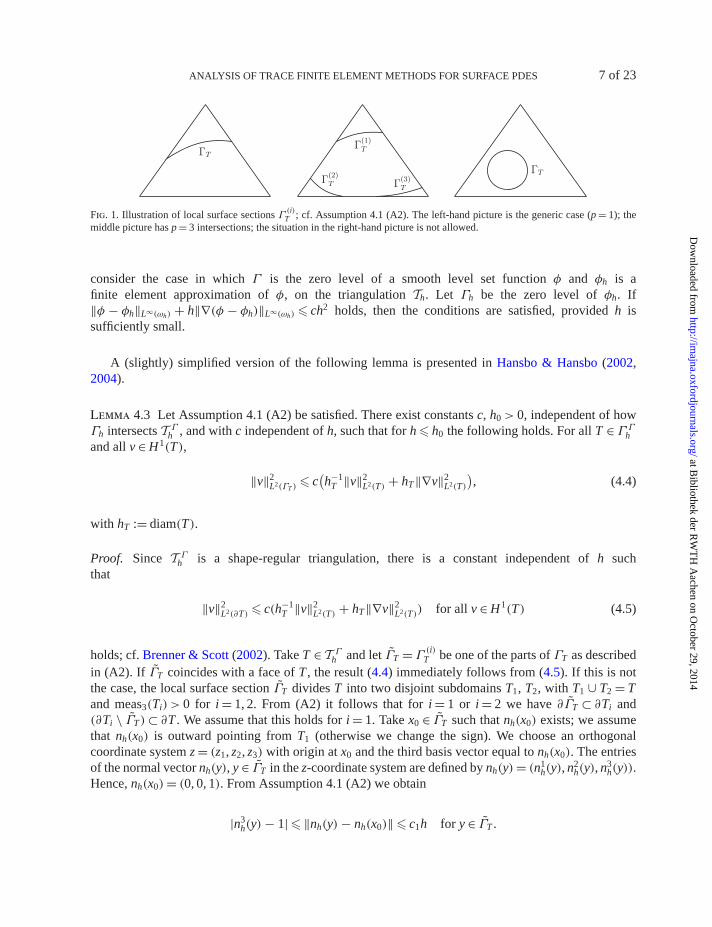
h has sufficient resolution for representing the surface Γ approximately. Condi-tion (A2) allows multiple intersections (namely p) of Γh with one tetrahedron T ∈ T Γ

h . An illus-tration for the two-dimensional case is shown in Fig. 1. We discuss three situations in whichAssumption 4.1 is satisfied. For the case Γh = Γ and with h sufficiently small, the conditionsin Assumption 4.1 hold. If Γh is a shape-regular triangulation, consisting of triangles with dia-meter O(h) and vertices on Γ , then for h sufficiently small the conditions are satisfied. Finally,

at Bibliothek der R

WT

H A



Dow

nloaded from



Fig. 1. Illustration of local surface sections Γ (i)T ; cf. Assumption 4.1 (A2). The left-hand picture is the generic case (p = 1); themiddle picture has p = 3 intersections; the situation in the right-hand picture is not allowed.

consider the case in which Γ is the zero level of a smooth level set function φ and φh is afinite element approximation of φ, on the triangulation Th. Let Γh be the zero level of φh. If‖φ − φh‖L∞(ωh) + h‖∇(φ − φh)‖L∞(ωh) � ch2 holds, then the conditions are satisfied, provided h issufficiently small.

A (slightly) simplified version of the following lemma is presented in Hansbo & Hansbo (2002,2004).

Lemma 4.3 Let Assumption 4.1 (A2) be satisfied. There exist constants c, h0 > 0, independent of howΓh intersects T Γ

h , and with c independent of h, such that for h � h0 the following holds. For all T ∈ Γ Γh

and all v ∈ H1(T),

‖v‖2L2(ΓT )

� c(h−1

T ‖v‖2L2(T) + hT‖∇v‖2

L2(T)

), (4.4)

with hT := diam(T).

Proof. Since T Γh is a shape-regular triangulation, there is a constant independent of h such

that

‖v‖2L2(∂T) � c(h−1

T ‖v‖2L2(T) + hT‖∇v‖2

L2(T)) for all v ∈ H1(T) (4.5)

holds; cf. Brenner & Scott (2002). Take T ∈ T Γh and let ΓT = Γ

(i)T be one of the parts of ΓT as described

in (A2). If ΓT coincides with a face of T , the result (4.4) immediately follows from (4.5). If this is notthe case, the local surface section ΓT divides T into two disjoint subdomains T1, T2, with T1 ∪ T2 = Tand meas3(Ti) > 0 for i = 1, 2. From (A2) it follows that for i = 1 or i = 2 we have ∂ΓT ⊂ ∂Ti and(∂Ti \ ΓT )⊂ ∂T . We assume that this holds for i = 1. Take x0 ∈ ΓT such that nh(x0) exists; we assumethat nh(x0) is outward pointing from T1 (otherwise we change the sign). We choose an orthogonalcoordinate system z = (z1, z2, z3) with origin at x0 and the third basis vector equal to nh(x0). The entriesof the normal vector nh(y), y ∈ ΓT in the z-coordinate system are defined by nh(y)= (n1

h(y), n2h(y), n3

h(y)).Hence, nh(x0)= (0, 0, 1). From Assumption 4.1 (A2) we obtain

|n3h(y)− 1| � ‖nh(y)− nh(x0)‖ � c1h for y ∈ ΓT .

at Bibliothek der R

WT

H A



Dow

nloaded from


8 of 23 A. REUSKEN

Thus there is a constant c such that, for h sufficiently small, 1 � n3h(y)

−1 � c holds a.e. on ΓT . Forv ∈ H1(T), we obtain

2∫

T1

v∂v

∂z3dz =

∫T1

divz

⎛⎝ 0

0v2

⎞⎠ dz =

∫∂T1

nT1 ·⎛⎝ 0

0v2

⎞⎠ dz

=∫ΓT

n3hv2 dz +

∫∂T1\ΓT

n3T1

v2 dz.

Using n3h(y)

−1 � c we obtain

∫ΓT

v2 dz � c

(∫T1

v∂v

∂z3dz −

∫∂T1\ΓT

n3Tv2 dz

)

� c(‖v‖L2(T)‖∇v‖L2(T) + ‖v‖2

L2(∂T)

)� c

(h−1

T ‖v‖2L2(T) + hT‖∇v‖2

L2(T)

),

where in the last inequality we used (4.5). Summing over the parts Γ (i)T , i = 1, . . . , p and using that p is

uniformly bounded, we obtain estimate (4.4). �

In the remainder we assume that h is sufficiently small. In particular, h � h0 as in Lemma 4.3 isassumed to be satisfied. As an easy.

Theorem 4.4 Let Assumption 4.1 be satisfied. Let Ih : C(ωh)→ Vh,m be the nodal interpolation. Thereexists a constant c, independent of h and of how Γh intersects T Γ

h , such that

minvh∈VΓ

h,m

(‖ue − vh‖L2(Γh) + h‖∇(ue − vh)‖L2(Γh)

)

� ‖ue − Ihue‖L2(Γh) + h‖∇(ue − Ihue)‖L2(Γh) � chm+1‖u‖Hm+1(Γ ) (4.6)

for all u ∈ Hm+1(Γ ) holds.

Proof. From u ∈ Hm+1(Γ ) it follows that ue ∈ Hm+1(ωh). Using Lemma 4.3 and standard error boundsfor the nodal interpolation Ih we obtain, with vh := Ihue ∈ Vh,m,

‖ue − vh‖2L2(Γh)

+ h2‖∇(ue − vh)‖2L2(Γh)

=∑

T∈T Γh

(‖ue − vh‖2L2(ΓT )

+ h2‖∇(ue − vh)‖2L2(ΓT )

)

� c∑

T∈T Γh

(h−1

T ‖ue − vh‖2L2(T) + (h2h−1

T + hT )‖∇(ue − vh)‖2L2(T)

+ h2hT‖∇2(ue − vh)‖2L2(T)

)� c

∑T∈T Γ

h

h2m+1‖ue‖2Hm+1(T) = ch2m+1‖ue‖2

Hm+1(ωh).

Using Assumption 4.1 (A1) and (3.8) with δ = c0h we obtain ‖ue‖2Hm+1(ωh)

� ch‖u‖2Hm+1(Γ )

, which com-pletes the proof. �

at Bibliothek der R

WT

H A



Dow

nloaded from



From the result in this theorem we conclude that for the trace space VΓh,m we have optimal approx-

imation error bounds under (very) mild conditions on the approximate surface Γh. If Γ and the exactsolution u are sufficiently smooth, we obtain an hm+1 bound as in (4.6) (for finite elements of degreem), provided Assumption 4.1 is satisfied. The latter essentially only requires the accuracy estimatedist(Γh,Γ )� ch for the approximate surface.

5. Finite element error bounds

In this section we prove optimal discretization error bounds both in the H1(Γh) and the L2(Γh) norm.For the discrete problem (2.5) such bounds for m = 1 (piecewise linear finite elements) are derived inDeckelnick et al. (2013). For the discrete problem (2.6) these error bounds for m = 1 are derived inOlshanskii et al. (2009). In both references it is assumed that Γh is a piecewise planar approximationof Γ with dist(Γh,Γ )� ch2. In this section we consider a more general setting with m � 1 and moregeneral approximate surfaces Γh. Furthermore, we present the error analysis of the two discretizationsin one unified setting, which reveals the main (theoretical) differences between the two methods.

In the analysis we need one further assumption, which quantifies the quality of Γh as an approxima-tion of Γ (‘geometric error’).

Assumption 5.1 We assume that Γh ⊂ Uδ0 is a Lipschitz surface without boundary and that the projec-tion p : Γh → Γ is a bijection. The corresponding unit normal field is defined a.e. on Γh and denoted bynh. We assume that the following holds, for a k � 1:

‖d‖L∞(Γh) � chk+1, (5.1)

‖n − nh‖L∞(Γh) � chk . (5.2)

These are the key assumptions we need in the analysis below. There is one further assumption weintroduce. On each Γh there holds a Poincaré inequality with a constant c = c(h). We assume that thisconstant is uniform w.r.t. h, i.e., we assume that there exists c, independent of h, such that

‖v‖L2(Γh) � c‖∇Γhv‖L2(Γh) for all v ∈ H1(Γh)/R. (5.3)

Remark 5.2 We discuss cases in which assumptions (5.1) and (5.2) are satisfied. Clearly, if Γh = Γ ,there is no geometric error, i.e., these assumptions are fulfilled with k = ∞. Consider the case in whichΓ is the zero level of a smooth level set function φ and φh is a finite element approximation of φ, onthe triangulation Th. Let Γh be the zero level of φh. If ‖φ − φh‖L∞(ωh) + h‖∇(φ − φh)‖L∞(ωh) � chk+1

holds, then conditions (5.1) and (5.2) are satisfied. In Demlow (2009) a method for constructing poly-nomial approximations to Γ is presented that satisfies conditions (5.1) and (5.2) (cf. Demlow, 2009,Proposition 2.3). In that method the exact distance function to Γ is needed.

Remark 5.3 It can be shown that under reasonable assumptions on Γh, the uniform Poincaré inequality(5.3) holds. We sketch a proof. Let v ∈ H1(Γh)/R be given. We define its lift to Γ by v(p(x))= v(x) forx ∈ Γh. We use a transformation formula

∫Γ(v)2 ds = ∫

Γhv2μh dsh, with μh as given in, e.g., Demlow

& Dziuk (2007). This μh satisfies (under reasonable assumptions on Γh) ‖1 − μh‖L∞(Γh) � ch2. Definecv := (1/|Γ |) ∫

Γv ds. Using

∫Γh

v dsh = 0 and the bound for ‖1 − μh‖L∞(Γh) we get |cv| � ch2‖v‖L2(Γh).

at Bibliothek der R

WT

H A



Dow

nloaded from


10 of 23 A. REUSKEN

For v := v − cv the Poincaré inequality on Γ holds. Combining these results we obtain

‖v‖L2(Γh) � c‖v‖L2(Γ ) � c(‖v‖L2(Γ ) + |cv|)� c‖∇Γ v‖L2(Γ ) + ch2‖v‖L2(Γh) � c‖∇Γhv‖L2(Γh) + ch2‖v‖L2(Γh),

from which, for h sufficiently small, the uniform estimate (5.3) follows.

We define the following projections:

Ph(x)= I − nh(x)nh(x)T, Ph(x)= I − nh(x)n(x)

T/(nh(x)Tn(x)), x ∈ Γh.

We collect a few results from Demlow & Dziuk (2007). The surface gradient of u ∈ H1(Γ ) can berepresented in terms of ∇Γhu

e as follows:

∇Γ u(p(x))= (I − d(x)H(x))−1Ph(x)∇Γhue(x) a.e. on Γh. (5.4)

For x ∈ Γh define

μh(x)= (1 − d(x)κ1(x))(1 − d(x)κ1(x))n(x)Tnh(x).

The integral transformation formula

μh(x) dsh(x)= ds(p(x)), x ∈ Γh (5.5)

holds, where dsh(x) and ds(p(x)) are the surface measures on Γh and Γ , respectively. From ‖n(x)−nh(x)‖2 = 2(1 − n(x)Tnh(x)) and Assumption 5.1 we obtain

‖1 − μh‖L∞(Γh) � chk+1, (5.6)

with a constant c independent of h. Using relations (5.4) and (5.5) we obtain

∫Γ

∇Γ u · ∇Γ v ds =∫Γh

Ah∇Γhue · ∇Γhv

e dsh for all u, v ∈ H1(Γ ), (5.7)

with Ah(x)=μh(x)Ph(x)(I − d(x)H(x))−2Ph(x). (5.8)

We introduce a compact notation for the bilinear forms used in (2.5) and (2.6):

ah(uh, vh) :=∫Γh

∇uh · ∇vh dsh, aΓh (uh, vh) :=∫Γh

∇Γhuh · ∇Γhvh dsh.

Furthermore, for the data error we introduce the notation

δf := fh − μhf e.

We now derive approximate Galerkin orthogonality relations for the discrete problems.

Lemma 5.4 Let u be the solution of the Laplace–Beltrami equation (2.2) and uh, uΓh ∈ VΓh,m be the solu-

tions of the discrete problems (2.5) and (2.6), respectively. Define Ah := PhAhPh, with Ah as in (5.8).

at Bibliothek der R

WT

H A



Dow

nloaded from



The following hold:

ah(ue − uh, vh)= Fh(vh) for all vh ∈ Vh,m,

with Fh(vh) :=∫Γh

(I − Ah)∇ue · ∇vh dsh −∫Γh

δf vh dsh; (5.9)

aΓh (ue − uΓh , vh)= FΓh (vh) for all vh ∈ Vh,m,

with FΓh (vh) :=∫Γh

(Ph − Ah)∇ue · ∇vh dsh −∫Γh

δf vh dsh. (5.10)

Proof. Take vh ∈ Vh,m. The function vh|Γh can be lifted on Γ by defining vlh(p(x)) := vh(x), x ∈ Γh. From

the definition of the discrete problem (2.5) and the transformation rule (5.7) we obtain

ah(uh, vh)=∫Γh

fhvh dsh =∫Γ

fvlh ds +

∫Γh

δf vh dsh

=∫Γ

∇Γ u · ∇Γ vlh ds +

∫Γh

δf vh dsh =∫Γh

Ah∇Γhue · ∇Γhvh ds +

∫Γh

δf vh dsh

=∫Γh

Ah∇ue · ∇vh ds +∫Γh

δf vh dsh,

where in the last equality we used that ∇Γhvh = Ph∇vh. Combining this with ah(ue, vh)=∫Γh

∇ue ·∇vh dsh we get the result in (5.9). Similar arguments can be used to derive (5.10):

aΓh (uΓh , vh)=

∫Γh


∫Γ

fvlh ds +

∫Γh

δf vh dsh

=∫Γh

Ah∇ue · ∇vh ds +∫Γh

δf vh dsh.

We combine this with aΓh (ue, vh)=

∫Γh

Ph∇ue · ∇vh dsh and thus obtain (5.10). �

Note that the only difference between the perturbation terms Fh and FΓh in (5.9) and (5.10) is in thematrices I − Ah and Ph − Ah. We derive bounds for the perturbation terms Fh and FΓh . We need someadditional notation, namely H2(Γ )e := {ve | v ∈ H2(Γ )}.Lemma 5.5 Let Assumption 5.1 be fulfilled and assume that the data error satisfies ‖δf ‖L2(Γh) �chk+s‖f ‖L2(Γ ) for an s ∈ [0, 1]. The following hold, with constants c independent of h:

|Fh(v)| � chk‖f ‖L2(Γ )

(‖v‖L2(Γh) + ‖∇v‖L2(Γh)

)for all v ∈ Vh,m + H2(Γ )e, (5.11)

|FΓh (v)| � chk+s‖f ‖L2(Γ )

(‖v‖L2(Γh) + ‖∇Γhv‖L2(Γh)

)for all v ∈ Vh,m + H2(Γ )e, (5.12)

|Fh(ve)| � chk+s‖f ‖L2(Γ )

(‖v‖L2(Γ ) + ‖∇Γ v‖L2(Γ )

)for all v ∈ H2(Γ ). (5.13)

Proof. For the second term in Fh(v) and FΓh (v) we obtain∣∣∣∣∫Γh

δf v dsh

∣∣∣∣ � ‖δf ‖L2(Γh)‖v‖L2(Γh) � chk+s‖f ‖L2(Γ )‖v‖L2(Γh). (5.14)

at Bibliothek der R

WT

H A



Dow

nloaded from


12 of 23 A. REUSKEN

Below, we delete the argument x ∈ Γh in the notation. Using (3.4), P(p(x))= P(x) and HP = PH , weobtain

(I − Ah)∇ue = (I − Ah)P(I − dH)∇Γ u(p(x)). (5.15)

We combine Ah = PhAhPh with the definition of Ah and with (5.1), (5.6), PhPh = Ph and obtain

‖Ah − Ph‖L∞(Γh) � chk+1. (5.16)

Hence, using (5.2) yields

‖(I − Ah)P‖L∞(Γh) � ‖(I − Ph)P‖L∞(Γh) + chk+1

� ‖P − Ph‖L∞(Γh) + chk+1 � chk . (5.17)

With the result in (5.15) we thus obtain∣∣∣∣∫Γh

(I − Ah)∇ue · ∇v dsh

∣∣∣∣ � chk‖∇Γ u(p(·))‖L2(Γh)‖∇v‖L2(Γh)

� chk‖∇Γ u‖L2(Γ )‖∇v‖L2(Γh) � chk‖f ‖L2(Γ )‖∇v‖L2(Γh), (5.18)

and combining this with the result in (5.14) completes the proof of (5.11). In the definition of FΓh (v) wehave the matrix Ph − Ah, instead of I − Ah. For the former we have (cf. (5.16)) ‖Ah − Ph‖L∞(Γh) � chk+1.Furthermore, we have

(Ph − Ah)∇ue · ∇v = Ph(Ph − Ah)∇ue · ∇v = (Ph − Ah)∇ue · ∇Γhv.

Similarly to (5.18), we obtain∣∣∣∣∫Γh

(Ph − Ah)∇ue · ∇v dsh

∣∣∣∣ � chk+1‖∇Γ u(p(·))‖L2(Γh)‖∇Γhv‖L2(Γh)

� chk+1‖f ‖L2(Γ )‖∇Γhv‖L2(Γh),

and combining this with the result in (5.14) we get the bound (5.12). We finally consider the estimate(5.13). We use (3.4) and thus obtain (cf. (5.15))

(I − Ah)∇ue · ∇ve = [(I − dH)P(I − Ah)P(I − dH)]∇Γ u(p(x)) · ∇Γ v(p(x)).

For the matrix in the square brackets we have (cf. (5.16)),

‖(I − dH)P(I − Ah)P(I − dH)‖L∞(Γh) � ‖P(I − Ph)P‖L∞(Γh) + chk+1.

Using P(I − Ph)P = PnhnTh P = (P − Ph)nhnT

h (P − Ph) and (5.2) we obtain ‖P(I − Ph)P‖L∞(Γh) � ch2k .From this it follows that the norm of the matrix in the square brackets is bounded by chk+1. Usingsimilar arguments as in the derivation of (5.12) above we then obtain the bound (5.13). �

Remark 5.6 We comment on the data error ‖δf ‖L2(Γh), with δf = fh − μhf e. For the choice fh = f e −(1/|Γh|)

∫Γh

f e dsh, which in practice often cannot be realized, we obtain, using (5.6), the data errorbound ‖δf ‖L2(Γh) � chk+1‖f ‖L2(Γ ). For this data error bound we only need f ∈ L2(Γ ), i.e., we avoid

at Bibliothek der R

WT

H A



Dow

nloaded from



higher-order regularity assumptions on f . Another, more feasible, possibility arises if we assume f to bedefined the neighbourhood Uδ0 of Γ . As an extension one can then use

fh(x)= f (x)− cf , cf := 1

|Γh|∫Γh

f dsh. (5.19)

Using∫Γ

f ds = 0, (5.1), (5.6) and a Taylor expansion we obtain |cf | � chk+1‖f ‖H1∞(Uδ0 )and ‖f −

μhf e‖L2(Γh) � chk+1‖f ‖H1∞(Uδ0 ). Hence, we get data error bound ‖δf ‖L2(Γh) � chk+1‖f ‖L2(Γ ) with c =

c(f )= c‖f ‖H1∞(Uδ0 )‖f ‖−1

L2(Γ )and a constant c independent of f . Thus in problems with smooth data,

f ∈ H1∞(Uδ0), the extension defined in (5.19) satisfies the condition on the data error in Lemma 5.5 with

s = 1. In less regular situations, s< 1 may be more realistic.

Note that for s> 0 the bound on FΓh in (5.12) is of higher order in h than the one for Fh in (5.11).This difference is reflected in the discretization error bounds derived below. For Fh(ve) the higher-orderbound in (5.13) is obtained by using the special structure of ve (namely constant in the normal direction).The latter bound is used in the proof of the L2 error bound in Theorem 5.8.

Theorem 5.7 Let Assumptions 4.1 and 5.1 be fulfilled. Assume that the data error satisfies ‖δf ‖L2(Γh) �chk+s‖f ‖L2(Γ ) for an s ∈ [0, 1]. Let uh and uΓh be the solutions of the discrete problems (2.5) and (2.6),respectively. The following error bounds hold, with a constant c independent of h and f :

‖∇(ue − uh)‖L2(Γh) � c(hm‖u‖Hm+1(Γ ) + hk‖f ‖L2(Γ )

), (5.20)

‖∇Γh(ue − uΓh )‖L2(Γh) � c

(hm‖u‖Hm+1(Γ ) + hk+s‖f ‖L2(Γ )

). (5.21)

Proof. Define eh := ue − uh and ψh := Ihue ∈ Vh,m. We consider the splitting

‖∇eh‖2L2(Γh)

= ah(eh, eh)= ah(eh, ue − ψh)+ Fh(ψh − ue)+ Fh(eh).

For the first two terms on the right-hand side we use (5.11) and the interpolation error bounds ofTheorem 4.4 and thus obtain

ah(eh, ue − ψh)+ Fh(ψh − ue)� c(‖∇eh‖L2(Γh) + hk‖f ‖L2(Γh))hm‖u‖Hm+1(Γ )

� 14‖∇eh‖2

L2(Γh)+ ch2m‖u‖2

Hm+1(Γ ) + ch2k‖f ‖2L2(Γh)

. (5.22)

For the third term we need the Poincaré inequality (5.3). Define cu = ∫Γh

ue dsh. Using∫Γ

u ds = 0 and(5.6) we obtain |cu| � chk+1‖u‖L2(Γ ) � chk+1‖f ‖L2(Γ ). Note that

∫Γh

eh − cu dsh = 0 holds, hence withthe Poincaré inequality we obtain

‖eh‖L2(Γh) � ‖eh − cu‖L2(Γh) + chk+1‖f ‖L2(Γ )

� c‖∇Γheh‖L2(Γh) + chk+1‖f ‖L2(Γ ) � c‖∇eh‖L2(Γh) + chk+1‖f ‖L2(Γ ),

and using this in estimate (5.11) yields

Fh(eh)� chk‖f ‖L2(Γ )(‖∇eh‖L2(Γh) + hk+1‖f ‖L2(Γ ))� 14‖∇eh‖2

L2(Γh)+ ch2k‖f ‖2

L2(Γ ).

at Bibliothek der R

WT

H A



Dow

nloaded from


14 of 23 A. REUSKEN

Combining this with the result in (5.22) proves the bound in (5.20). The result in (5.21) follows withvery similar arguments. Define eΓh = ue − uΓh , and consider the splitting

‖∇ΓheΓh ‖2

L2(Γh)= aΓh (e

Γh , eΓh )= aΓh (e

Γh , ue − ψh)+ FΓh (ψh − ue)+ FΓh (e

Γh ).

Note that ‖∇Γh(ue − ψh)‖L2(Γh) � ‖∇(ue − ψh)‖L2(Γh), and hence for bounding the interpolation error we

can use Theorem 4.4. We can repeat the arguments used above. Since in the bound for FΓh (v) in (5.12)we have a term hk+s (instead of hk) we get the factor hk+s in the bound (5.21). �

The result in this theorem yields optimal H1-error bounds for both methods, and also for the case ofhigher-order finite elements (m � 2). Of course, this optimal bound is obtained only if the approximationerror term, which is of order hm, is not dominated by the geometric error term, which is of order hk andhk+s, respectively. Assume s = 1; cf. Remark 5.6. For the case k = m (which typically holds in case oflinear finite elements, i.e., m = 1), we see that for the method in (2.5) the geometric error is of the sameorder as the approximation error, whereas for the method (2.6) the geometric error is of higher order.For the method in (2.6) and m � 2 we get the optimal order of convergence hm even if we only havek = m − 1. The method (2.5) does not have this property.

We apply a duality argument to obtain an L2(Γh)-error bound. In this analysis the estimate (5.13) isused.

Theorem 5.8 Let Assumptions 4.1 and 5.1 be fulfilled. Assume that the data error satisfies ‖δf ‖L2(Γh) �chk+s‖f ‖L2(Γ ) for an s ∈ [0, 1]. Let uh and uΓh be the solutions of the discrete problems (2.5) and (2.6),respectively. The following error bounds hold, with a constant c independent of h and f :

‖ue − uh‖L2(Γh) � c(hm+1‖u‖Hm+1(Γ ) + hk+s‖f ‖L2(Γ )

), (5.23)

‖ue − uΓh ‖L2(Γh) � c(hm+1‖u‖Hm+1(Γ ) + hk+s‖f ‖L2(Γ )

). (5.24)

Proof. Define eh := ue − uh and let elh be the lift of eh|Γh on Γ and ce := ∫

Γel

h ds. Consider the problem:Find w ∈ H1(Γ ) with

∫Γ

w ds = 0 such that∫Γ

∇Γw · ∇Γ v ds =∫Γ

(elh − ce)v ds for all v ∈ H1(Γ ). (5.25)

The solution w satisfies w ∈ H2(Γ ) and ‖w‖H2(Γ ) � c‖elh‖L2(Γ )/R with ‖el

h‖L2(Γ )/R := ‖elh − ce‖L2(Γ ). We

take ψh = Ihwe ∈ Vh,m and with Ah = PhAhPh we obtain

‖elh‖2

L2(Γ )/R =∫Γ

∇Γw · ∇Γ (elh − ce) ds =

∫Γ

∇Γw∇Γ elh ds

=∫Γh

Ah∇Γheh · ∇Γhwe dsh =

∫Γh

∇eh · ∇we dsh +∫Γh

∇eh · (Ah − I)∇we dsh

= ah(eh, we − ψh)+ Fh(ψh − we)+ Fh(we)+

∫Γh

∇eh · (Ah − I)∇we dsh. (5.26)

We consider the four terms in (5.26). Using the interpolation error bound in Theorem 4.4 (with m = 1),the error bound in Theorem 5.7 and ‖w‖H2(Γ ) � c‖el

h‖L2(Γ )/R we obtain

ah(eh, we − ψh)� c(hm+1‖u‖Hm+1(Γ ) + hk+1‖f ‖L2(Γ ))‖elh‖L2(Γ )/R.

at Bibliothek der R

WT

H A



Dow

nloaded from



For the second term we use (5.11) and the interpolation error bound (with m = 1), which yields

Fh(ψh − we)� chk+1‖f ‖L2(Γ )‖elh‖L2(Γ )/R.

For the third term we use (5.13) and obtain

Fh(we)� chk+s‖f ‖L2(Γ )‖w‖H1(Γ ) � chk+s‖f ‖L2(Γ )‖el

h‖L2(Γ )/R. (5.27)

For the last term we use (5.15) (with u replaced by w) and (5.17), which yields

∫Γh

∇eh · (Ah − I)∇we dsh � chk‖∇eh‖L2(Γh)‖∇Γw‖L2(Γ )

� c(hm+k‖u‖Hm+1(Γ ) + h2k‖f ‖L2(Γ ))‖elh‖L2(Γ )/R.

Using these bounds in (5.26) yields

‖elh‖L2(Γ )/R � c

(hm+1‖u‖Hm+1(Γ ) + hk+s‖f ‖L2(Γ )

). (5.28)

Now note that

|ce| =∣∣∣∣∫Γ

u − ulh ds

∣∣∣∣ =∣∣∣∣∫Γ

ulh ds

∣∣∣∣ =∣∣∣∣∫Γh

(μh − 1)uh dsh

∣∣∣∣ � chk+1‖f ‖L2(Γ ),

and thus

‖eh‖L2(Γh) � c‖elh‖L2(Γ ) � c‖el

h‖L2(Γ )/R + chk+1‖f ‖L2(Γ ),

and combining this with (5.28) completes the proof of (5.23). The result (5.24) can be proved with verysimilar arguments. A proof of (5.24) for m = k = 1 is given in Olshanskii et al. (2009). �

Note that the bounds in (5.23) and (5.24) are the same. We have an optimal error if k + s � m + 1holds. If we have an optimal data approximation error, i.e., s = 1 (cf. Remark 5.6), we need k � m toobtain an optimal L2-error bound of order hm+1. Inspection of the proof above shows that the factorhk+s in (5.23) originates (only) from the estimate (5.27). All other geometric error terms are of orderhk+1. In the proof of (5.24) the term FΓh (w

e) has to be bounded. For this the estimate (5.12) is used.Inspection of the proof of the latter estimate reveals that the factor hk+s in the bound in (5.12) cannot beimproved if we use the special choice v = we. Thus in both error bounds, (5.23) and (5.24), we get thesame geometric error term of order hk+s.

6. Conditioning of the stiffness matrix

In this section we address linear algebra aspects of the discretizations in (2.5) and (2.6). The dis-crete solution is determined by using the standard nodal basis of the (outer) finite element space Vh,m.This nodal basis and the corresponding nodes are denoted by {φi}1�i�N and {xi}1�i�N , respectively.Hence, Vh,m = span{(φi)|ωh | 1 � i � N} and dim(Vh,m)= N . By construction we have span{(φi)|Γh | 1 �i � N} = VΓ

h,m. In relation to the linear algebra, a key point is that in general the {(φi)|Γh}1�i�N are not

at Bibliothek der R

WT

H A



Dow

nloaded from


16 of 23 A. REUSKEN

independent, hence these do not form a basis of the trace space VΓh,m. This can be illustrated by sim-

ple examples; cf. Olshanskii & Reusken (2010). The representation vh = ∑Ni=1 Viφi, vh ∈ Vh,m induces

the isomorphism vh → V := (Vi)1�i�N ∈ RN . The vector corresponding to wh ∈ Vh,m is denoted by W .

We introduce the mass and stiffness matrices:

〈MV , W〉 =∫Γh

vhwh dsh for all vh, wh ∈ Vh,m, (6.1)

〈AV , W〉 =∫Γh

∇vh · ∇wh dsh for all vh, wh ∈ Vh,m, (6.2)

〈AΓ V , W〉 =∫Γh

∇Γhvh · ∇Γhwh dsh for all vh, wh ∈ Vh,m. (6.3)

If {(φi)|Γh}1�i�N are dependent, there exists V ∈ RN , V |= 0 such that vh = ∑N

i=1 Viφi = 0 on Γh. Thisimplies 〈MV , V 〉 = 0 and thus M is singular. Furthermore, vh|Γh = 0 implies (∇Γhvh)|Γh = 0 and thus〈AΓ V , V 〉 = 0, hence AΓ is singular. This indicates that the conditioning properties of the mass matrixM and the stiffness matrix AΓ are different from those of standard finite element discretizations ofelliptic problems. In Olshanskii & Reusken (2010) this conditioning issue is studied. We outline a fewimportant results. In numerical experiments it is observed that for the Laplace–Beltrami equation dis-cretized with linear trace finite elements on an approximate surface Γh that is obtained as the zero levelof a piecewise linear level set function, the mass matrix M has one zero eigenvalue (within machineaccuracy) and the stiffness matrix AΓ has two zero eigenvalues. The effective condition number isdefined as the quotient of the largest and the smallest nonzero eigenvalue. Typically, both the diag-onally scaled mass matrix D−1

M M and the diagonally scaled stiffness matrix D−1AΓ AΓ have effective

condition numbers that behave like h−2. In Olshanskii & Reusken (2010) a rather technical analysis ispresented that gives a theoretical explanation of these conditioning properties. The analysis is only forthe two-dimensional case (i.e., Γ is a curve) and uses technical assumptions related to how Γh inter-sects the local triangulation T Γ

h . An example of such an assumption is that the relative size of the setof vertices in T Γ

h , having a certain maximal distance to Γh, gets smaller if this distance gets smaller(for precise statements we refer the reader to Olshanskii & Reusken, 2010). In the recent paper Bur-man et al. (2013), a stabilization technique for (2.6) is introduced, which improves the conditioningproperties of AΓ .

The discretization (2.5) is more stable than (2.6) in the sense that ‖∇vh‖L2(Γh) � ‖∇Γhvh‖L2(Γh) holds.In relation to this, note that vh|Γh = 0 does not necessarily imply that (∇vh)|Γh = 0 holds. Based on this,one might expect a better conditioning of the matrix A compared to AΓ . This is indeed observed innumerical experiments; cf. Section 7. In this section we derive conditioning properties of the stiffnessmatrix A for the case m = 1, i.e., linear finite elements. Using an elementary analysis it is shown that asuitably scaled A has a condition number that behaves like h−2 (on the space orthogonal to the constant),independently of how Γh intersects T Γ

h . Such a robustness property w.r.t. the geometry does not hold forthe scaled stiffness matrix AΓ . As a simple corollary we obtain a conditioning result for a shifted massmatrix; cf. Theorem 6.4.

In the analysis we use (global) inverse estimates. Therefore, in the remainder of this section weassume that the following holds.

Assumption 6.1 The local triangulation T Γh is quasi-uniform.

at Bibliothek der R

WT

H A



Dow

nloaded from



We consider m = 1 and use the notation Vh := Vh,1. In Remark 6.5 we comment on m � 2. For anode xi, let T (xi) be the set of all tetrahedra T ∈ T Γ

h that contain xi. Define

δT := |ΓT ||T | h, T ∈ T Γ

h , di :=∑

T∈T (xi)

δT , 1 � i � N .

(Recall ΓT = Γh ∩ T .) We introduce a weighted L2(ωh) norm,

‖v‖2δ,ωh

=∑

T∈T Γh

δT

∫T

v2 dx,

and a related scaled vector norm,

‖V‖2D := 〈DV , V 〉, D := diag(di).

From the fact that ∇φi · ∇φi is constant on each T ∈ T (xi) with value ∼ h−2 it follows that D is uni-formly spectrally equivalent to diag(A). Hence, the scaling with D that is used below can be replaced bya scaling with diag(A). The constants used in the lemma and theorems below are independent of h andof how Γh intersects the local triangulation T Γ

h .

Lemma 6.2 There are constants c1 > 0 and c2 such that

c1h3‖V‖2D � ‖vh‖2

δ,ωh� c2h3‖V‖2

D for all vh ∈ Vh.

Proof. We use the compact notation ∼ to represent inequalities in both directions with constants inde-pendent of h and of how Γh intersects ωh. The set of vertices of T is denoted by V(T). For vh ∈ Vh wehave Vi = vh(xi) and using the quasi-uniformity of T Γ

h we obtain

∫T

v2h dx ∼ |T |

∑xi∈V(T)

vh(xi)2 ∼ h3

∑xi∈V(T)

V 2i .

This implies

‖vh‖2δ,ωh

=∑

T∈T Γh

δT

∫T

v2h dx ∼ h3

∑T∈T Γ

h

δT

∑xi∈V(T)

V 2i

= h3N∑

i=1

⎛⎝ ∑

T∈T (xi)

δT

⎞⎠ V 2

i = h3N∑

i=1

diV2i = h3‖V‖2

D,

and thus the result holds. �

Theorem 6.3 There are constants c1 > 0 and c2 such that

c1h2‖V‖2D � 〈AV , V 〉 � c2‖V‖2

D for all V ∈ RN with

∫Γh

vh ds = 0.

at Bibliothek der R

WT

H A



Dow

nloaded from


18 of 23 A. REUSKEN

Proof. We first consider the upper bound. Note that, using an inverse inequality on T we obtain

〈AV , V 〉 =∫Γh

∇vh · ∇vh ds �∑

T∈T Γh

|ΓT | ‖∇vh‖2L∞(T) � c

∑T∈T Γ

h

h−2 |ΓT ||T | ‖vh‖2

L2(T)

= ch−3∑

T∈T Γh

δT

∫T

v2h dx = ch−3‖vh‖2

δ,ωh� c‖V‖2

D,

where in the last inequality we used Lemma 6.2.We now consider the lower bound. Using Lemma 6.2 we obtain

h2‖V‖2D � ch−1‖vh‖2

δ,ωh= ch−1

∑T∈T Γ

h

δT

∫T

v2h dx. (6.4)

Take a T ∈ T Γh . Let ξ ∈ T , η ∈ ΓT be such that |vh(x)| � |vh(ξ)| for all x ∈ T and |vh(η)| � |vh(x)| for all

x ∈ ΓT . From vh(ξ)= vh(η)+ (ξ − η) · ∇vh|T it follows that |vh(ξ)|2 � c(|vh(η)|2 + h2‖∇vh|T‖2). Usingthis we obtain

h−1δT

∫T

v2h dx � |ΓT | |vh(ξ)|2 � c(|ΓT ||vh(η)|2 + |ΓT |h2‖∇vh|T‖2)

� c

(∫ΓT

v2h ds + h2

∫ΓT

‖∇vh‖2 ds

).

Summing over T ∈ T Γh and using the Poincaré inequality (5.3) (which holds for vh with

∫Γh

vh dsh = 0),we obtain

h−1∑

T∈T Γh

δT

∫T

v2h dx � c

(∫Γh

v2h ds + h2

∫Γh

‖∇vh‖2 ds

)

� c

(∫Γh

‖∇Γhvh‖2 ds + h2∫Γh

‖∇vh‖2 ds

)� c

∫Γh

‖∇vh‖2 ds = c〈AV , V 〉. (6.5)

Combining this with the result in (6.4) completes the proof. �

As an immediate consequence of this theorem we obtain for the spectral condition number in thespace orthogonal to the one-dimensional kernel (corresponding to the constant function), denoted byκ∗(·),

κ∗(D−1A)� ch−2. (6.6)

We derive a result for a shifted mass matrix.

Theorem 6.4 There are constants c1, c2 > 0 such that for all α � 0,

c1(min{2h2,α} + αh2)‖V‖2D � 〈MV , V 〉 + α〈AV , V 〉 � c2(h

2 + α)‖V‖2D

for all V ∈ RN with

∫Γh

vh ds = 0.

at Bibliothek der R

WT

H A



Dow

nloaded from



Proof. First we consider the upper bound. Note that

〈MV , V 〉 =∫Γh

v2h ds �

∑T∈T Γ

h

|ΓT |‖vh‖2L∞(T) � ch−1

∑T∈T Γ

h

δT

∫T

v2h ds

= ch−1‖vh‖2δ,ωh

� ch2‖V‖2D.

In combination with Theorem 6.3 this yields the upper bound. For the lower bound we use the result in(6.5) and in Lemma 6.2 and thus obtain

〈MV , V 〉 + h2〈AV , V 〉 =∫Γh

v2h ds + h2

∫Γh

‖∇vh‖2 ds � ch−1‖vh‖2δ,ωh

� c0h2〈DV , V 〉,

with a constant c0 > 0. Using spectral inequalities for symmetric positive definite matrices we haveM + h2A � c0h2D. From this and the lower bound in Theorem 6.3 we obtain

M + αA = M +( α

2h2

)h2A + 1

2αA � min

{1,

α

2h2

}(M + h2A)+ 1

2αA

� c0 min{

1,α

2h2

}h2D + c1αh2D � c(min{2h2,α} + αh2)D,

which proves the lower bound. �

Thus, we have the following bound for the spectral condition number:

κ∗(D−1(M + αA))� ch2 + α

min{2h2,α} + αh2. (6.7)

For α→ ∞ we get the same bound as in (6.6). For α ↓ 0 the bound tends to infinity. This cannotbe avoided, since the mass matrix M can be singular (also in the space orthogonal to the constant),as explained above. More interesting is the case α � ch2 with c> 0. Then the bound takes the formch−2(α/(1 + α)). Hence, if α∼ h2, we get a uniform (i.e., independent of h) condition number boundand if α∼ h, we get a bound of the form ch−1. The case α∼ h2 is typical if a time-dependent surfacediffusion problem is considered in which, for the time discretization, an implicit Euler method is usedwith Δt ∼ h2. If, for such a time-dependent problem one uses Crank–Nicolson with Δt ∼ h, this resultsin a linear system with α ∼ h.

Remark 6.5 We comment on the case of higher-order finite elements, i.e., m � 2. Inspection of theproofs shows that the estimates in Lemma 6.2 and the upper bound in Theorem 6.3 also hold ifm � 2 is considered. The lower bound in Theorem 6.3, however, does not hold in general. Thisbecomes clear from the following example. Consider a two-dimensional setting with a domain ω=[0, 1] × [−1, 1] which is subdivided into a few triangles with vertices only on y = −1 or y = 1. We takeΓh = [0, 1] × {0}. We choose the P2 finite element function v(x, y)= αy2 + (x − 1

2 ) with α� 1. For thisfunction we have ‖v‖L2(ω) ∼ α,

∫Γh

v ds = 0, ∇v = (1, 2αy)T and thus ‖∇v‖L2(Γh) = 1. The lower boundin Theorem 6.3 scales with h2‖V‖2

D ∼ ‖v‖2L2(ω)

∼ α2, whereas 〈AV , V 〉 = ‖∇v‖2L2(Γh)

= 1 holds. Hence,we conclude that the first inequality c1h2‖V‖2

D � 〈AV , V 〉 in Theorem 6.3 cannot hold for this simpleexample. The key point in this example is that we cannot control the values of vh on ω by its values andgradient on Γh.

at Bibliothek der R

WT

H A



Dow

nloaded from


20 of 23 A. REUSKEN

7. Numerical experiments

In this section we present the results of a numerical experiment. As a test problem we consider theLaplace–Beltrami equation on the unit sphere:

−ΔΓ u = f on Γ ,

with Γ = {x ∈ R3 | ‖x‖2 = 1} and Ω = (−2, 2)3.

The source term f is taken such that the solution is given by

u(x)= 1

‖x‖3(3x2

1x2 − x32), x = (x1, x2, x3) ∈Ω .

Using the representation of u in spherical coordinates one can verify that u is an eigenfunction of −ΔΓ :

u(r,φ, θ)= sin(3φ) sin3 θ , −ΔΓ u = 12u =: f (r,φ, θ). (7.1)

The right-hand side f satisfies the compatibility condition∫Γ

f ds = 0, likewise does u. Note that u andf are constant along normals at Γ .

A family {Tl}l�0 of tetrahedral triangulations of Ω is constructed as follows. We triangulate Ω bystarting with a uniform subdivision into 48 tetrahedra with mesh size h0 = √

3. Then we apply an adap-tive red–green refinement algorithm (implemented in the software package DROPS: DROPS package)in which in each refinement step the tetrahedra that contain Γ are refined such that on level l = 1, 2, . . . ,we have

hT �√

3 2−l =: hl for all T ∈ Tl with T ∩ Γ |= ∅.

The family {Tl}l�0 is consistent and shape regular. The local triangulation T Γh is quasi-uniform. The

interface Γ is the zero level of ϕ(x) := ‖x‖2 − 1. Let ϕh := Ih(ϕ) where Ih is the standard nodal inter-polation operator on Tl, which maps into the space of piecewise linears Vh,1. The discrete interface isgiven by Γhl := {x ∈Ω |ϕh(x)= 0}. In the experiments below we only consider this interface approx-imation, which satisfies the conditions in Assumption 5.1 with k = 1. Note that this discrete interfacetriangulation is very shape irregular. For the extension fh of f we take the constant extension of f alongthe normals at Γ , i.e., we take fh(r,φ, θ)= f (1,φ, θ)+ ch, with f (r,φ, θ) as in (7.1) and ch such that∫Γh

fh dsh = 0. For the computation of the integrals∫

T fhφh dsh we use a quadrature rule that is exact upto order five. The extension ue of u is given by ue(r,φ, θ) := u(1,φ, θ)= u(r,φ, θ) (since u is constantalong nΓ ).

We consider the discrete problems (2.5) and (2.6) with solutions uh and uΓh , respectively.

Experiment 7.1 (Discretization errors for k = m = 1.) For the discretization of u we use the finiteelement space VΓ

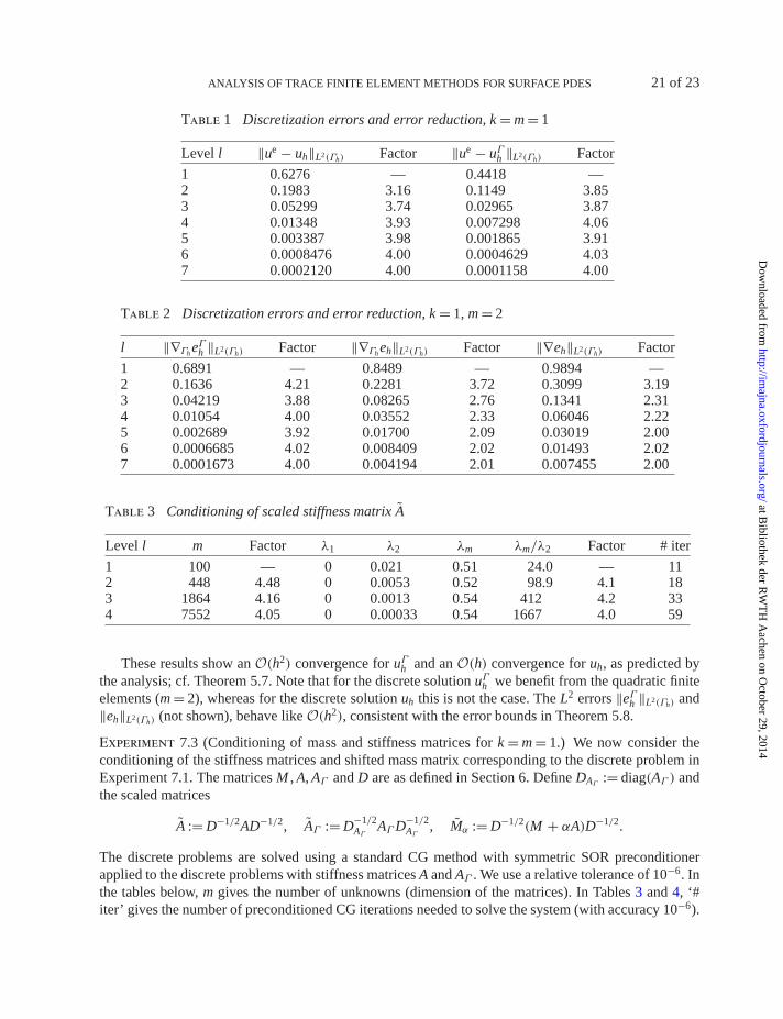
h,1, i.e., the trace of piecewise linear finite element functions. The discretization errorsin the L2(Γh) norm are given in Table 1.

These results clearly show the h2 behaviour as predicted by the analysis; cf. Theorem 5.8. We alsoobserve that the discretization error for uΓh is about a factor 2 smaller than for uh.

Experiment 7.2 (Discretization errors for k = 1, m = 2.) We keep the piecewise planar approximationΓh of Γ (i.e., k = 1), but for the discretization of u we now use the finite element space VΓ

h,2, i.e., thetrace of piecewise quadratic finite element functions (m = 2). For the two methods the H1 discretizationerrors are given in Table 2. We use the notation eh := ue − uh, eΓh := ue − uΓh .

at Bibliothek der R

WT

H A



Dow

nloaded from



Table 1 Discretization errors and error reduction, k = m = 1

Level l ‖ue − uh‖L2(Γh) Factor ‖ue − uΓh ‖L2(Γh) Factor

1 0.6276 — 0.4418 —2 0.1983 3.16 0.1149 3.853 0.05299 3.74 0.02965 3.874 0.01348 3.93 0.007298 4.065 0.003387 3.98 0.001865 3.916 0.0008476 4.00 0.0004629 4.037 0.0002120 4.00 0.0001158 4.00

Table 2 Discretization errors and error reduction, k = 1, m = 2

l ‖∇ΓheΓh ‖L2(Γh) Factor ‖∇Γheh‖L2(Γh) Factor ‖∇eh‖L2(Γh) Factor

1 0.6891 — 0.8489 — 0.9894 —2 0.1636 4.21 0.2281 3.72 0.3099 3.193 0.04219 3.88 0.08265 2.76 0.1341 2.314 0.01054 4.00 0.03552 2.33 0.06046 2.225 0.002689 3.92 0.01700 2.09 0.03019 2.006 0.0006685 4.02 0.008409 2.02 0.01493 2.027 0.0001673 4.00 0.004194 2.01 0.007455 2.00

Table 3 Conditioning of scaled stiffness matrix A

Level l m Factor λ1 λ2 λm λm/λ2 Factor # iter

1 100 — 0 0.021 0.51 24.0 — 112 448 4.48 0 0.0053 0.52 98.9 4.1 183 1864 4.16 0 0.0013 0.54 412 4.2 334 7552 4.05 0 0.00033 0.54 1667 4.0 59

These results show an O(h2) convergence for uΓh and an O(h) convergence for uh, as predicted bythe analysis; cf. Theorem 5.7. Note that for the discrete solution uΓh we benefit from the quadratic finiteelements (m = 2), whereas for the discrete solution uh this is not the case. The L2 errors ‖eΓh ‖L2(Γh) and‖eh‖L2(Γh) (not shown), behave like O(h2), consistent with the error bounds in Theorem 5.8.

Experiment 7.3 (Conditioning of mass and stiffness matrices for k = m = 1.) We now consider theconditioning of the stiffness matrices and shifted mass matrix corresponding to the discrete problem inExperiment 7.1. The matrices M , A, AΓ and D are as defined in Section 6. Define DAΓ := diag(AΓ ) andthe scaled matrices

A := D−1/2AD−1/2, AΓ := D−1/2AΓ AΓD−1/2

AΓ , Mα := D−1/2(M + αA)D−1/2.

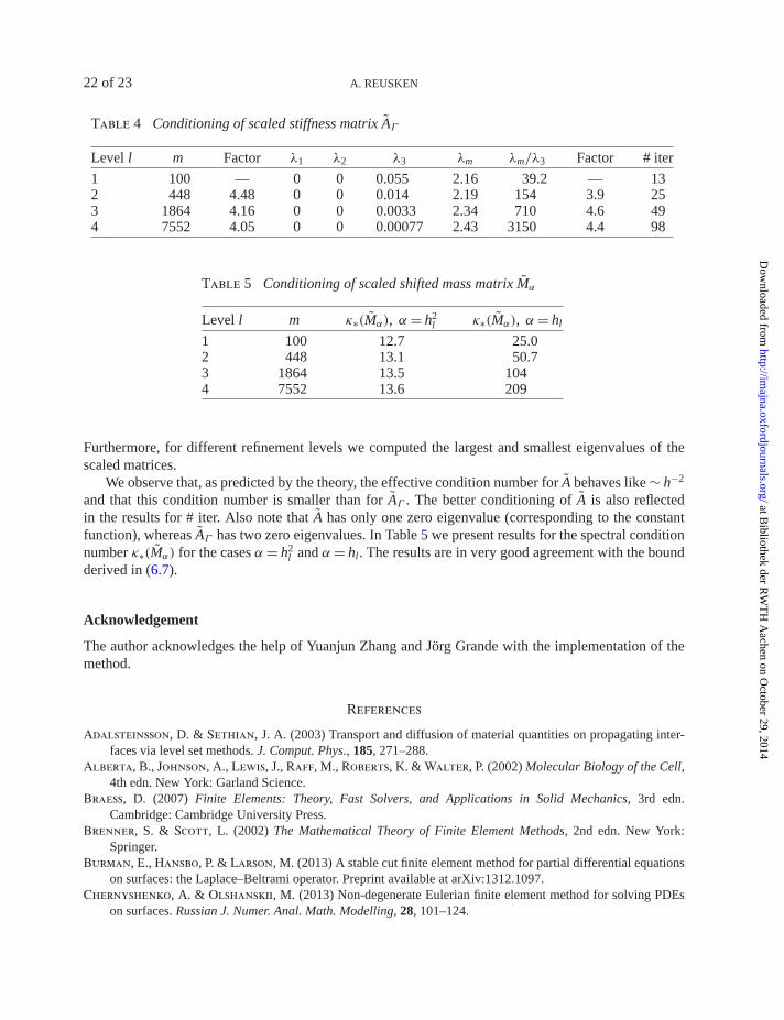
The discrete problems are solved using a standard CG method with symmetric SOR preconditionerapplied to the discrete problems with stiffness matrices A and AΓ . We use a relative tolerance of 10−6. Inthe tables below, m gives the number of unknowns (dimension of the matrices). In Tables 3 and 4, ‘#iter’ gives the number of preconditioned CG iterations needed to solve the system (with accuracy 10−6).

at Bibliothek der R

WT

H A



Dow

nloaded from


22 of 23 A. REUSKEN

Table 4 Conditioning of scaled stiffness matrix AΓ

Level l m Factor λ1 λ2 λ3 λm λm/λ3 Factor # iter

1 100 — 0 0 0.055 2.16 39.2 — 132 448 4.48 0 0 0.014 2.19 154 3.9 253 1864 4.16 0 0 0.0033 2.34 710 4.6 494 7552 4.05 0 0 0.00077 2.43 3150 4.4 98

Table 5 Conditioning of scaled shifted mass matrix Mα

Level l m κ∗(Mα), α = h2l κ∗(Mα), α= hl

1 100 12.7 25.02 448 13.1 50.73 1864 13.5 1044 7552 13.6 209

Furthermore, for different refinement levels we computed the largest and smallest eigenvalues of thescaled matrices.

We observe that, as predicted by the theory, the effective condition number for A behaves like ∼ h−2

and that this condition number is smaller than for AΓ . The better conditioning of A is also reflectedin the results for # iter. Also note that A has only one zero eigenvalue (corresponding to the constantfunction), whereas AΓ has two zero eigenvalues. In Table 5 we present results for the spectral conditionnumber κ∗(Mα) for the cases α = h2

l and α = hl. The results are in very good agreement with the boundderived in (6.7).

Acknowledgement

The author acknowledges the help of Yuanjun Zhang and Jörg Grande with the implementation of themethod.

References

Adalsteinsson, D. & Sethian, J. A. (2003) Transport and diffusion of material quantities on propagating inter-faces via level set methods. J. Comput. Phys., 185, 271–288.

Alberta, B., Johnson, A., Lewis, J., Raff, M., Roberts, K. & Walter, P. (2002) Molecular Biology of the Cell,4th edn. New York: Garland Science.

Braess, D. (2007) Finite Elements: Theory, Fast Solvers, and Applications in Solid Mechanics, 3rd edn.Cambridge: Cambridge University Press.

Brenner, S. & Scott, L. (2002) The Mathematical Theory of Finite Element Methods, 2nd edn. New York:Springer.

Burman, E., Hansbo, P. & Larson, M. (2013) A stable cut finite element method for partial differential equationson surfaces: the Laplace–Beltrami operator. Preprint available at arXiv:1312.1097.

Chernyshenko, A. & Olshanskii, M. (2013) Non-degenerate Eulerian finite element method for solving PDEson surfaces. Russian J. Numer. Anal. Math. Modelling, 28, 101–124.

at Bibliothek der R

WT

H A



Dow

nloaded from



Deckelnick, K., Elliott, C. & Ranner, T. (2013) Unfitted finite element methods using bulk meshes for surfacepartial differential equations. Preprint available at arXiv:1312.2905.

Demlow, A. (2009) Higher-order finite element methods and pointwise error estimates for elliptic problems onsurfaces. SIAM J. Numer. Anal., 47, 805–827.

Demlow, A. & Dziuk, G. (2007) An adaptive finite element method for the Laplace–Beltrami operator on implic-itly defined surfaces. SIAM J. Numer. Anal., 45, 421–442.

Demlow, A. & Olshanskii, M. (2012) An adaptive surface finite element method based on volume meshes. SIAMJ. Numer. Anal., 50, 1624–1647.

DROPS package http://www.igpm.rwth-aachen.de/DROPS/.Dziuk, G. (1988) Finite elements for the Beltrami operator on arbitrary surfaces. Partial Differential Equations

and Calculus of Variations (S. Hildebrandt & R. Leis eds). Lecture Notes in Mathematics, vol. 1357. Berlin:Springer, pp. 142–155.

Dziuk, G. & Elliott, C. (2007) Finite elements on evolving surfaces. IMA J. Numer. Anal., 27, 262–292.Dziuk, G. & Elliott, C. (2010) An Eulerian approach to transport and diffusion on evolving implicit surfaces.

Comput. Visual Sci., 13, 17–28.Elliott, C. M., Stinner, B., Styles, V. & Welford, R. (2011) Numerical computation of advection and diffusion

on evolving diffuse interfaces. IMA J. Numer. Anal., 31, 786–812.Grande, J. & Reusken, A. (2014) A higher-order finite element method for partial differential equations on

surfaces (submitted). Preprint 401, IGPM, RWTH Aachen University.Greer, J. B. (2008) An improvement of a recent Eulerian method for solving PDEs on general geometries. J. Sci.

Comput., 29, 321–352.Gross, S. & Reusken, A. (2011) Numerical Methods for Two-Phase Incompressible Flows. Berlin: Springer.Hansbo, A. & Hansbo, P. (2002) An unfitted finite element method, based on Nitsche’s method, for elliptic inter-

face problems. Comput. Methods Appl. Mech. Engrg., 191, 5537–5552.Hansbo, A. & Hansbo, P. (2004) A finite element method for the simulation of strong and weak discontinuities in

solid mechanics. Comput. Methods Appl. Mech. Engrg., 193, 3523–3540.Olshanskii, M. A. & Reusken, A. (2010) A finite element method for surface PDEs: matrix properties. Numer.

Math., 114, 491–520.Olshanskii, M. & Reusken, A. (2013) Error analysis of a space-time finite element method for solving PDEs on

evolving surfaces. IGPM Preprint No 376, Department of Mathematics, RWTH Aachen University. Acceptedfor publication in SIAM J. Numer. Anal.

Olshanskii, M. A., Reusken, A. & Grande, J. (2009) A finite element method for elliptic equations on surfaces.SIAM J. Numer. Anal., 47, 3339–3358.

Olshanskii, M., Reusken, A. & Xu, X. (2014a) An Eulerian space-time finite element method for diffusionproblems on evolving surfaces. SIAM J. Numer. Anal., 52, 1354–1377.

Olshanskii, M., Reusken, A. & Xu, X. (2014b) A stabilized finite element method for advection–diffusion equa-tions on surfaces. IMA J. of Numer. Anal., 34, 732–758.

Ranner, T. (2013) Computational surface partial differential equations. Ph.D. Thesis, University of Warwick.Sethian, J. A. (1996) Theory, algorithms, and applications of level set methods for propagating interfaces. Acta

Numer., 5, 309–395.Xu, J.-J. & Zhao, H.-K. (2003) An Eulerian formulation for solving partial differential equations along a moving

interface. J. Sci. Comput., 19, 573–594.

at Bibliothek der R

WT

H A



Dow

nloaded from

http://www.igpm.rwth-aachen.de/DROPS/


Analysis of trace ﬁnite element methods for surface ...

Documents

Transcript of Analysis of trace ﬁnite element methods for surface ...