Generalized finite element method enrichment functions forcurvedsingularities in 3D fracture mechanics problems

J.P. Pereira†, C.A. Duarte†∗, X. Jiao†† and D. Guoy‡

November 28, 2008

†Department of Civil & Environmental Engineering,

University of Illinois at Urbana-Champaign, 205 North Mathews Ave., Urbana, IL 61801, U.S.A..††Department of Applied Mathematics and Statistics, Stony Brook University, Stony Brook, NY 11794-3600.

‡Center for Simulation of Advanced Rockets,

University of Illinois at Urbana-Champaign, 1304 West Springfield Avenue, Urbana, IL 61801, U.S.A..

Abstract

This paper presents a study of generalized enrichment functions for three-dimensional curved crackfronts. Two coordinate systems used in the definition of singular curved crack front enrichment functionsare analyzed. In the first one, a set of Cartesian coordinate systems defined along the crack front is used.In the second case, the geometry of the crack front is approximated by a set of curvilinear coordinatesystems. A description of the computation of derivatives ofenrichment functions and curvilinear basevectors is presented. The coordinate systems are automatically defined using geometrical informationprovided by an explicit representation of the crack surface. A detailed procedure to accurately evaluatethe surface normal, conormal and tangent vectors along curvilinear crack fronts in explicit crack surfacerepresentations is also presented. An accurate and robust definition of orthonormal vectors along crackfronts is crucial for the proper definition of enrichment functions. Numerical experiments illustrate theaccuracy and robustness of the proposed approaches.

Keywords: Partition of unity methods; Generalized/Extended finite element method; Three-dimensionalfracture mechanics; Crack front enrichments.

1 Introduction

Three-dimensional computational fracture mechanics simulations are of great importance in industry. Lifeprediction of engine components, structural members of aircraft fuselage, and pipeline joints are examplesof industrial problems in which 3D computational fracture mechanics analysis is broadly applied. Thestandard finite element method (FEM) has been used for several decades in the assessment of such industrialproblems. The application of the FEM to this class of problems faces several issues regarding changesin mesh topology and excessive computational cost. These difficulties are usually due to remeshing andthe need for highly refined meshes in the crack surface region. Such modifications in the mesh are oftenrequired because of crack surface fitting and accuracy of thesolution. Partition of unity methods, such asthe generalized finite element method (GFEM) [1, 4, 16, 23, 33], are promising candidates to overcome

∗Corresponding author: caduarte@illinois.edu

1

these difficulties. However, in three-dimensional fracture analysis with partition of unity-based methods,the accurate representation of curvilinear crack fronts isstill a challenging task.

Partition of unity methods have been successfully applied to fracture mechanics problems. The main ideaof modeling fracture mechanics problems with these methodsis to represent discontinuities and singularitiesof the solution through custom-built shape functions. The discontinuity far from crack tip/front can be easilyrepresented by step functions [19, 20, 35] or high-order step functions [6, 28], depending on the polynomialorder used in the approximation of the continuous part of thesolution. In order to represent the singularityof the solution in linear elastic fracture mechanics problems, enrichment functions based on the analyticalsolution of the elasticity around the crack front are usually applied [2, 4, 5, 20, 22, 24, 28, 35]. Theapplication of partition of unity methods to cohesive fracture models and corresponding enrichments can befound in, for example, [17, 18, 31, 32, 40, 41, 42].

In the mid 1990’s, many researchers applied the partition ofunity concept and the asymptotic expansionnear the crack tip to represent discontinuities and singularities in two-dimensional crack problems. Theidea of including the near crack tip asymptotic expansion inpartition of unity approximation was firstlyintroduced by Duarte and Oden in [7, 22, 24]. They used the partition of unity concept in thehp-cloudmethod to represent the singularity and discontinuity of the solution in the approximation. Asymptoticexpansions were introduced in the element-free Galerkin method by Fleming et al. [9]. Two approacheswere utilized to enrich the element-free Galerkin approximation with the first terms of the near tip expansion.The first approach adds the first terms of the near-tip asymptotic expansion of the displacement field to thetrial functions. The second approach expands the linear basis used in the moving least squares method[13, 14] by including the term

√r multiplied by trigonometric functions. By using the partition of unity

concept, Belytschko and Black [2] applied the second enrichment approach introduced in [9] in a finiteelement framework. The approach introduced by Belytschko and Black [2] was improved by Moes et al.[19]. They applied Heaviside functions to those nodes with support intersecting the crack surface but notthe crack tip, and the asymptotic expansion for those nodes with support intersecting the crack tip.

Duarte et al. [4] extended the enrichment approach used in [7, 22, 24] for a three-dimensional finiteelement framework. The asymptotic expansion was utilized to model straight reentrant corners using thepartition of unity concept. In [5], Duarte et al. applied the same enrichment approach to arbitrary crackfronts in three-dimensional dynamic crack propagation. Sukumar et al. [35] and Moes et al. [20] extendedthe approach presented in [19] for three-dimensional crack modeling of planar and non-planar crack surfaceswith curved crack fronts, respectively.

To our best knowledge, the references available in the literature regarding three-dimensional analysisof crack problems using partition of unity-based methods, give very little attention to the description andconstruction of enrichment functions for curved fronts. Moreover, in all existing approaches, the effects ofcrack front curvatures in the asymptotic expansion are not considered in the enrichment functions.

The aim of this paper is to analyze two approaches for describing and enriching three-dimensional curvedcrack fronts. The first approach is based on a piecewise linear description of the crack front. The secondone uses a piecewise quadratic description while taking into consideration the derivatives of the base vectorsin the computation of the gradient of the asymptotic expansion. Another contribution of this paper is adetailed procedure to evaluate surface normal, conormal and tangent vectors along a curved crack front.These vectors are utilized in the definition of base vectors which, in turn, define the crack front enrichmentfunctions. An accurate and robust definition of these crack front vectors is crucial for the proper definitionof crack front enrichment functions.

The outline of this paper is as follows. In the following Section we briefly review the construction ofGFEM shape functions and present the enrichment functions used with the proposed piecewise linear andquadratic crack front geometrical approximations. Section 3 presents a procedure to accurately evaluate

2

the normal, conormal and tangent vectors along the crack front in an explicit crack surface representation.The crack front description using linear and quadratic approximations and the transformation maps for theirrespective enrichment functions are discussed in Section4. The numerical experiments presented in Section5 illustrate the robustness and accuracy of the proposed three-dimensional enrichment techniques. Finally,Section6 outlines the conclusions and highlights the main contributions of the present study.

2 Generalized FE shape functions

The generalized FEM [1, 4, 16, 23, 33] can be regarded as a FEM with shape functions built using theconcept of a partition of unity. In this section, we focus on the construction of GFEM shape functions usedin the neighborhood of a three-dimensional crack front. Details on the GFEM can be found in many papersavailable in the literature. Here, we follow the formulation and notation introduced in [28].

In the GFEM, a shape functionφα i is built from the product of a linear finite element shape function, ϕα ,and an enrichment function,Lα i ,

φα i(xxx) = ϕα(xxx)Lα i(xxx) (no summation onα) (1)

whereα is the index of a nodexxxα in the finite element mesh. The GFEM shape functionφα i is defined onωα = xxx∈Ω : ϕα(xxx) 6= 0, the support of the partition of unity functionϕα . In the case of a finite elementpartition of unity, the supportωα (often called cloud) is given by the union of the finite elements sharinga vertex nodexxxα [4]. The selection of enrichment functions depends on the local behavior of the solutionuuu of the problem of interest over the cloudωα . In the case of linear elastic fracture mechanics problems,the enrichment functions used at cloudsωα that intersect the crack front are taken from the asymptoticexpansion of the elasticity solution near a crack front [4, 5, 22, 24, 28].

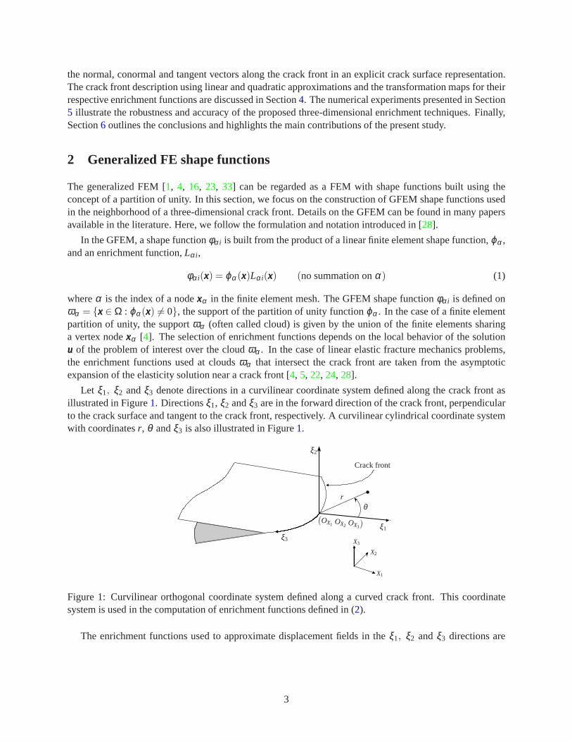
Let ξ1, ξ2 andξ3 denote directions in a curvilinear coordinate system defined along the crack front asillustrated in Figure1. Directionsξ1, ξ2 andξ3 are in the forward direction of the crack front, perpendicularto the crack surface and tangent to the crack front, respectively. A curvilinear cylindrical coordinate systemwith coordinatesr, θ andξ3 is also illustrated in Figure1.

θ

ξ2

r

X2

X3

X1

Crack front

ξ3

ξ1

(

OX1 OX2 OX3

)

Figure 1: Curvilinear orthogonal coordinate system definedalong a curved crack front. This coordinatesystem is used in the computation of enrichment functions defined in (2).

The enrichment functions used to approximate displacementfields in theξ1, ξ2 andξ3 directions are

3

given by [4, 5, 22, 24, 28]

Lξ1α1(r,θ ) =

√r

[

(κ− 12)cos

θ2− 1

2cos

3θ2

]

Lξ2α1(r,θ ) =

√r

[

(κ +12)sin

θ2− 1

2sin

3θ2

]

Lξ3α1(r,θ ) =

√r sin

θ2

(2)

Lξ1α2(r,θ ) =

√r

[

(κ +32)sin

θ2

+12

sin3θ2

]

Lξ2α2(r,θ ) =

√r

[

(κ− 32)cos

θ2

+12

cos3θ2

]

Lξ3α2(r,θ ) =

√r sin

3θ2

where the material constantκ = 3−4ν andν is Poisson’s ratio. This assumes plane strain conditions, whichis in general a good approximation far from crack front ends.The above enrichment functions correspondto the first term of the modesI and II , and to the first and second terms of the modeIII components ofthe asymptotic expansion of elasticity solution around a straight crack front, far from the vertices and fora traction-free flat crack surface [36]. It should be noted, as indicated by the superscripts, thatdifferentenrichment functions are used in (2) for each component of the displacement vector. This leads to a totalof six additional degrees of freedom at a nodeα enriched with these functions. In contrast, the enrichmentfunctions used in, e.g., [3, 20, 34, 35], lead, in 3D, to twelve degrees of freedom per node since fourenrichment functions are used for each component of the displacement vector. In the approach proposed in(2), only two enrichments are used to enrich each component of the displacement vector. The performanceof these two choices of enrichment functions is analyzed in [25].

The enrichment functions (2) are defined in a coordinate system located along the crack front as illus-trated in Figure1. Thus, they must be transformed to the global Cartesian coordinate system(X1,X2,X3)prior to their use in the definition of GFEM shape functions in(1). Details are presented in Sections4.1.1and4.2.2.

In our computations, the crack surface is represented by flattriangles with straight edges [28] as illus-trated in Figures5 and6. Thus, curved crack fronts are approximated by straight line segments. The fidelityof this approximation can be controlled by simply using a finer triangulation of the crack surface. This pro-cess isindependentof the GFEM mesh and does not change the problem size [28]. This paper focus on theconstruction of crack front coordinate systems and corresponding enrichment functions using geometricalinformation provided by this crack surface representation. It should be noted that the coordinate systemsproposed here can be used to define enrichment functions for several classes of problems. In particular, itcan be applied to the case of cohesive cracks, and other non-linear fracture mechanics problems. The onlymodification required is to replace (2) by appropriate enrichment functions.

3 Crack front base vectors

This section presents computational procedures to determine orthonormal base vectors at vertices along acrack front. These crack front vectors are the surface normal vector, curve tangent vector and conormalvector computed at each vertex of the front using the geometrical description of the crack surface. Thesevectors define a local Cartesian coordinate system at each crack front vertex. Moreover, they are utilized

4

in the construction of curved hexahedra along the crack front. These elements, in turn, define curvilinearcoordinate systems, as described in Section4.2.1.

3.1 Evaluation of the crack front normals, tangent and conormal vectors

The crack front normal, tangent and conormal vectors are used in the definition of the branch functionenrichments (2) as well as in the extraction of stress intensity factors (SIFs). A good estimation of thesecrack front vectors is worthwhile to obtain an accurate approximation of the solution around the crack frontand, consequently, an accurate SIF extraction.

In the level sets method applied to partition of unit-based methods for crack problems [20, 34, 35], thecrack front vectors of the implicit representation of the crack surface are computed based on the gradients ofthe front and surface level sets. However, according to Duflot [8], this approach may lead to an inaccuraterepresentation of the crack front because the orthogonality of the surface and front level set gradients doesnot always hold.

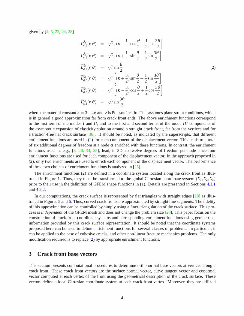
In this paper, the crack surface is represented by an explicit three-dimensional triangulation. Figure2illustrates an arbitrary crack surface and the normal, tangent and conormal vectors along the crack front.More details about this crack surface representation can befound in [28]. The evaluation of the crackfront vectors for this explicit representation of the cracksurface, by design, guarantees the accuracy andorthogonality of the crack front vectors. The following sequence of procedures describes how to evaluatethe crack front normals for an explicit crack surface representation.

Figure 2: Non-planar crack surface and normals, tangents and conormals along the crack front representedby black, yellow and red arrows, respectively..

Evaluation of the normal vectors using medial quadric The computation of normal vectors at vertices offacets representing aC0 surface is not a trivial task. The vertex normals along the crack front are ill-definedand an algorithm based on a naive approach, e.g. the average of normals of the facets sharing a vertex,may lead to inaccurate estimates of normals for coarse meshes or near geometric singularities. Figure

5

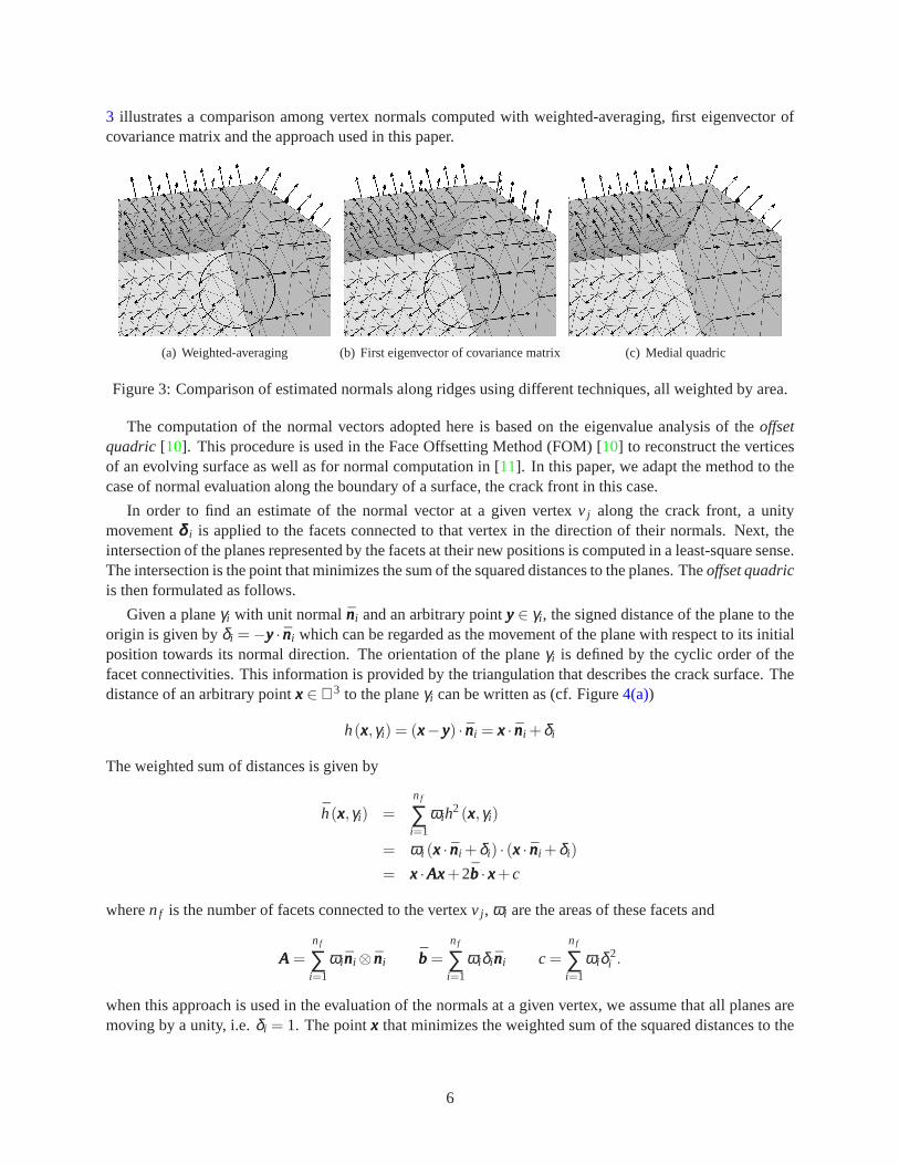
3 illustrates a comparison among vertex normals computed with weighted-averaging, first eigenvector ofcovariance matrix and the approach used in this paper.

(a) Weighted-averaging (b) First eigenvector of covariance matrix (c) Medial quadric

Figure 3: Comparison of estimated normals along ridges using different techniques, all weighted by area.

The computation of the normal vectors adopted here is based on the eigenvalue analysis of theoffsetquadric [10]. This procedure is used in the Face Offsetting Method (FOM)[10] to reconstruct the verticesof an evolving surface as well as for normal computation in [11]. In this paper, we adapt the method to thecase of normal evaluation along the boundary of a surface, the crack front in this case.

In order to find an estimate of the normal vector at a given vertex v j along the crack front, a unitymovementδδδ i is applied to the facets connected to that vertex in the direction of their normals. Next, theintersection of the planes represented by the facets at their new positions is computed in a least-square sense.The intersection is the point that minimizes the sum of the squared distances to the planes. Theoffset quadricis then formulated as follows.

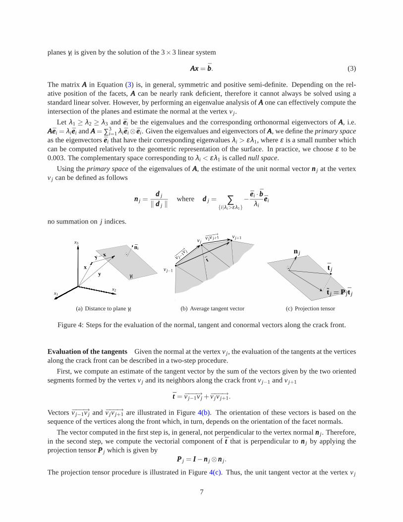
Given a planeγi with unit normalnnni and an arbitrary pointyyy∈ γi , the signed distance of the plane to theorigin is given byδi =−yyy· nnni which can be regarded as the movement of the plane with respect to its initialposition towards its normal direction. The orientation of the planeγi is defined by the cyclic order of thefacet connectivities. This information is provided by the triangulation that describes the crack surface. Thedistance of an arbitrary pointxxx∈ℜ3 to the planeγi can be written as (cf. Figure4(a))

h(xxx,γi) = (xxx−yyy) · nnni = xxx· nnni +δi

The weighted sum of distances is given by

h(xxx,γi) =nf

∑i=1

ωih2(xxx,γi)

= ωi (xxx· nnni +δi) · (xxx· nnni +δi)

= xxx·AAAxxx+2bbb·xxx+c

wherenf is the number of facets connected to the vertexv j , ωi are the areas of these facets and

AAA =nf

∑i=1

ωi nnni⊗ nnni bbb =nf

∑i=1

ωiδi nnni c =nf

∑i=1

ωiδ 2i .

when this approach is used in the evaluation of the normals ata given vertex, we assume that all planes aremoving by a unity, i.e.δi = 1. The pointxxx that minimizes the weighted sum of the squared distances to the

6

planesγi is given by the solution of the 3×3 linear system

AAAxxx = bbb. (3)

The matrixAAA in Equation (3) is, in general, symmetric and positive semi-definite. Depending on the rel-ative position of the facets,AAA can be nearly rank deficient, therefore it cannot always be solved using astandard linear solver. However, by performing an eigenvalue analysis ofAAA one can effectively compute theintersection of the planes and estimate the normal at the vertexv j .

Let λ1 ≥ λ2 ≥ λ3 and eeei be the eigenvalues and the corresponding orthonormal eigenvectors ofAAA, i.e.AAAeeei = λi eeei andAAA= ∑3

i=1 λi eeei⊗ eeei . Given the eigenvalues and eigenvectors ofAAA, we define theprimary spaceas the eigenvectorseeei that have their corresponding eigenvaluesλi > ελ1, whereε is a small number whichcan be computed relatively to the geometric representationof the surface. In practice, we chooseε to be0.003. The complementary space corresponding toλi < ελ1 is callednull space.

Using theprimary spaceof the eigenvalues ofAAA, the estimate of the unit normal vectornnn j at the vertexv j can be defined as follows

nnn j =ddd j

‖ ddd j ‖where ddd j = ∑

i|λi>ελ1− eeei · bbb

λieeei

no summation onj indices.

x1x2

x3

xy γi

y−xni

(a) Distance to planeγi

v j+1−−−→v jv j+1

−−−→

v j−1vj

t

v j

v j−1

(b) Average tangent vector

t j

t j = P j t j

n j

(c) Projection tensor

Figure 4: Steps for the evaluation of the normal, tangent andconormal vectors along the crack front.

Evaluation of the tangents Given the normal at the vertexv j , the evaluation of the tangents at the verticesalong the crack front can be described in a two-step procedure.

First, we compute an estimate of the tangent vector by the sumof the vectors given by the two orientedsegments formed by the vertexv j and its neighbors along the crack frontv j−1 andv j+1

ttt =−−−→v j−1v j +−−−→v jv j+1.

Vectors−−−→v j−1v j and−−−→v jv j+1 are illustrated in Figure4(b). The orientation of these vectors is based on thesequence of the vertices along the front which, in turn, depends on the orientation of the facet normals.

The vector computed in the first step is, in general, not perpendicular to the vertex normalnnn j . Therefore,in the second step, we compute the vectorial component ofttt that is perpendicular tonnn j by applying theprojection tensorPPP j which is given by

PPP j = III −nnn j ⊗nnn j .

The projection tensor procedure is illustrated in Figure4(c). Thus, the unit tangent vector at the vertexv j

7

can be written as follows

ttt j =ttt j

‖ ttt j ‖wherettt j = PPP j ttt j and no summation implied inj indices.

Evaluation of the conormals Once the normal and tangent are computed for a given vertexv j , the conor-mal is simply the cross product between them.

bbb j = nnn j × ttt j

no summation implied inj indices.

4 Crack front approximation and enrichment functions

This section presents two approaches to build approximations to the crack front curvilinear coordinate sys-tem defined in Section2. The computation of corresponding enrichment functions and their derivativeswith respect to global coordinate directions is also presented. In the first approach, the curved crack frontcoordinate system is approximated by a set of Cartesian coordinate systems while in the second case a set ofcurvilinear (quadratic) approximations is used.It should be noted that the shape and location of the crackfront is dictated not only by the triangulation used to represent the crack surface but also by the coordinatesystems used in the computation of the enrichment functions(2). Thesegeometricalapproximations aredenoted hereafter aslinear andquadraticapproximations of the crack front geometry. They should notbeconfused with the polynomial order of GFEM shape functions.In both approaches proposed here, eachnodexxxα enriched with functions (2) defines its own coordinate system. Since the enrichment functions usedat distinct cloudsωα do not have to be the same, this does not pose any problem for the GFEM. The twoprocedures are presented in Sections4.1and4.2, respectively.

A key ingredient of both procedures is the computation of unity vectors along the crack front that arenormal to the crack surface, tangent to the crack front or oriented in the conormal (forward) direction of thecrack front, as presented in Section3.1.

4.1 Linear approximation of crack front geometry

In this approach, the crack front curvilinear coordinate system is approximated by a set of Cartesian coor-dinate systems. Each cloudωα enriched with functions (2) defines a rectangular coordinate system approx-imately tangent to the crack front as described below. Thus,the crack front shape is approximated by a setof linear segments.

The procedure to define the Cartesian coordinate system(ξ1,ξ2,ξ3) used to compute enrichment func-tions (2) at a cloudωα associated with a finite element nodexxxα can be described as follows1

• Find the closest crack front vertexv j to nodexxxα . This procedure can be efficiently implemented usinggeometric predicates.

• Compute at front vertexv j unity vectorseee1, eee2, eee3 oriented in the conormal direction to the crackfront, normal direction to the crack surface and tangent direction to the crack front, respectively. Thecomputation of these vectors is described in Section3.1. They are taken as the base vectors of thecoordinate system.

1A crack front vertex may be referenced using its index,v j , or its coordinates,vvv j .

8

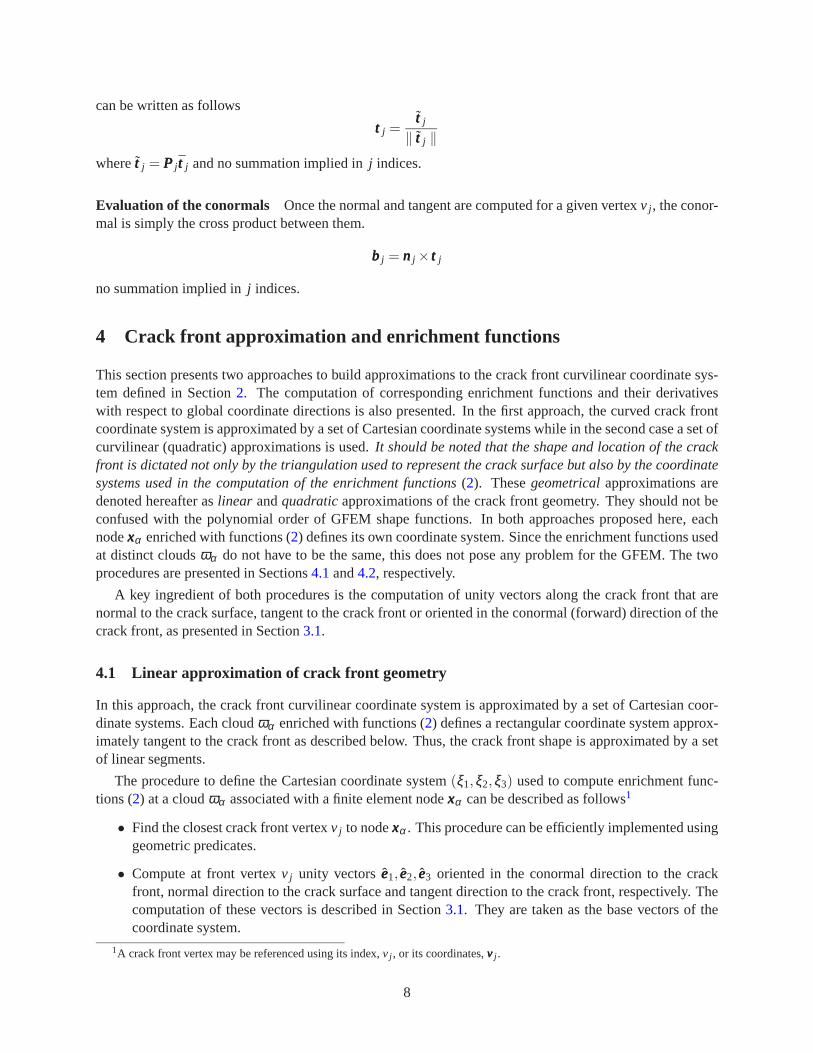
• Let v j−1 andv j+1 denote the index of the two crack front vertex nodes connected to vertex nodev j

(cf. Figure4(b)). The originOOO of the coordinate system is taken as the average of the position vectorsof these three crack front vertex nodes.

Figure5 illustrates a crack front Cartesian coordinate system(ξ1,ξ2,ξ3) built as described above. Astraight cylindrical coordinate system(r,θ ,ξ3) can be defined using(ξ1,ξ2,ξ3), as described below. Thissystem is used in the computation of the singular enrichments (2). Thus, these functions represent a locallystraight crack front in the cloudωα . Since clouds along crack fronts are very small due to mesh refinement,this approximation of a curved crack front is acceptable. Numerical experiments presented in Section5confirm this hypothesis.

Linear Approximation

xxxαeee1

eee3

v j+1

Crack Front Geometry

eee2

v j

v j−1

Crack Surface Geometry

OOO

Figure 5: Base vectors and origin of a Cartesian coordinate system used for the computation of enrichmentfunctions for nodexxxα . Each node with singular enrichment defines its own Cartesian coordinate system. Asa result, the crack front shape is approximated by a set of linear segments.

4.1.1 Transformation of enrichment functions to global coordinates

Enrichment functionsLξ jα i(r,θ ), i = 1,2, j = 1,2,3, computed in the cylindrical coordinate system are trans-

formed to the global Cartesian system(X1,X2,X3) as follows.

DefineL

ξ jα i(ξ1,ξ2,ξ3) = L

ξ jα i T−1

a (ξ1,ξ2,ξ3) i = 1,2, j = 1,2,3 (4)

where “” denotes composition of two functions. The transformation

T−1a : (ξ1,ξ2,ξ3) 7−→ (r,θ ,ξ3)

is given by

rθξ3

=

√

ξ 21 +ξ 2

2

arctan(ξ2

ξ1)

ξ3

(5)

9

The Jacobian of this transformation is given by

[(JJJ−1

a

)

i j

]

=

[∂ r i

∂ ξ j

]

=

cos(θ ) sin(θ ) 0

−1r

sin(θ )1r

cos(θ ) 0

0 0 1

(6)

wherer i , i = 1,2,3, denote cylindrical coordinatesr, θ andξ3, respectively.

Next defineL

ξ jα i(X1,X2,X3) = L

ξ jα i T−1

b (X1,X2,X3) i = 1,2, j = 1,2,3 (7)

where the transformationT−1

b : (X1,X2,X3) 7−→ (ξ1,ξ2,ξ3)

is given by

ξ1

ξ2

ξ3

= RRR−1

b

X1−O1

X2−O2

X3−O3

(8)

Above,(O1,O2,O3) are the coordinates of the originOOO of the crack coordinate system andRRR−1b ∈ℜ3×ℜ3

is a rotation matrix with rows given by the base vectorseeei , i = 1,2,3.

The Jacobian of this transformation is given by

(JJJ−1

b

)

i j =∂ ξi

∂Xj=(RRR−1

b

)

i j

The displacement vectors(Lξ1α1, L

ξ2α1, L

ξ3α1) and(Lξ1

α2, Lξ2α2, L

ξ3α2) have components in the crack front coor-

dinate directionsξ1,ξ2,ξ3 and thus must be transformed to the global Cartesian system(X1,X2,X3) using

LX1α1 LX1

α2LX2

α1 LX2α2

LX3α1 LX2

α2

= RRRb

Lξ1α1 Lξ1

α2

Lξ2α1 Lξ2

α2

Lξ3α1 Lξ3

α2

(9)

whereRRRb = (RRR−1b )T . FunctionsL

Xjα i , i = 1,2, j = 1,2,3, can now be used in (1) to define GFEM shape

functions. The computation of their derivatives with respect to global coordinate directions is presented inAppendixA. These functions are the same as those in Equation (11) of [28]. They are also presented inSection 4 of [4].

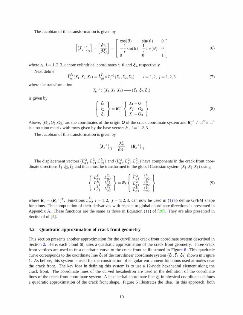
4.2 Quadratic approximation of crack front geometry

This section presents another approximation for the curvilinear crack front coordinate system described inSection2. Here, each cloudωα uses a quadratic approximation of the crack front geometry.Three crackfront vertices are used to fit a quadratic curve to the crack front as illustrated in Figure6. This quadraticcurve corresponds to the coordinate lineξ3 of the curvilinear coordinate system(ξ1,ξ2,ξ3) shown in Figure1. As before, this system is used for the construction of singular enrichment functions used at nodes nearthe crack front. The key idea in defining this system is to use a12-node hexahedral element along thecrack front. The coordinate lines of the curved hexahedron are used in the definition of the coordinatelines of the crack front coordinate system. A hexahedral coordinate lineξ3 in physical coordinates definesa quadratic approximation of the crack front shape. Figure6 illustrates the idea. In this approach, both

10

the crack front and the crack surface can be curved. The only assumption we make regarding the shapeof the crack surface is that,within a cloudωα , the surface is flat in the crack front conormal directionξ1.Transformation of coordinates between this system and the global coordinate system(X1,X2,X3) is thendefined using the shape functions and nodal coordinates of the hexahedral element. The construction of thecurved hexahedron can be fully automated without difficulty. It should be noted the 12-node hexahedra areused only to define curvilinear coordinate systems. They do not add any degrees of freedom to the problem.Details are presented below.

In this section,ξ1, ξ2 andξ3 may denote either a coordinate in the master coordinate system of a brickor the corresponding coordinate line in physical space(X1,X2,X3). The meaning is clear from the context.

X (ξ1,ξ2,

ξ3)

X3, eee3

X2, eee2

ξ1

ξ3

ξ2eee2

eee1

X1, eee1

X (0,0,

ξ3)

eee3r

Figure 6: Non-planar crack surface and coordinate system for curved front enrichment.

4.2.1 Construction of hexahedra along a curved crack front

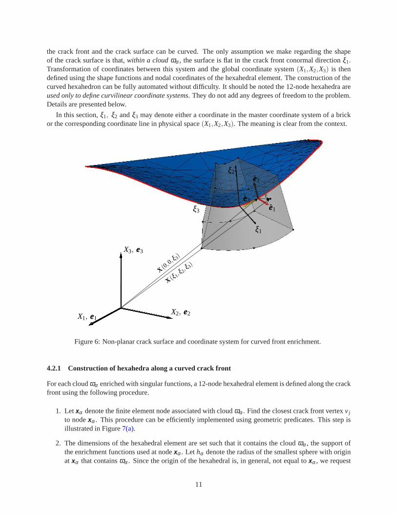
For each cloudωα enriched with singular functions, a 12-node hexahedral element is defined along the crackfront using the following procedure.

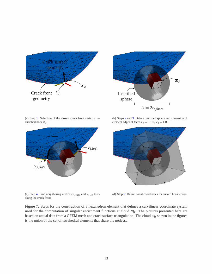
1. Letxxxα denote the finite element node associated with cloudωα . Find the closest crack front vertexv j

to nodexxxα . This procedure can be efficiently implemented using geometric predicates. This step isillustrated in Figure7(a).

2. The dimensions of the hexahedral element are set such thatit contains the cloudωα , the support ofthe enrichment functions used at nodexxxα . Let hα denote the radius of the smallest sphere with originat xxxα that containsωα . Since the origin of the hexahedral is, in general, not equalto xxxα , we request

11

that the hexahedral contains a sphere of radius given by

rsphere=‖ −−→vvv jxxxα ‖+hα

where‖ −−→vvv jxxxα ‖ is the distance from the closest crack front vertex,vvv j , to the finite element nodexxxα .This step is illustrated in Figure7(b).

3. Define the dimension,lh, of the edges of the hexahedral cross-section atξ3 = −1.0, ξ3 = 0.0, andξ3 = 1.0. The hexahedral cross-section is squared andlh is taken aslh = 2rsphere.

4. Starting from vertexv j , select the two closest vertices,vj, right andvj, left, along the crack front direc-tions ξ3 = 1 andξ3 = −1, respectively, such that they are located outside of the sphere with radiusrsphereand originvvv j . This step is illustrated in Figure7(c).

5. Compute at front verticesvj, left, v j andvj, right the triadbbb, nnn, ttt oriented in the conormal direction of thecrack front, normal to the crack surface and tangent to the crack front, respectively. The computationof these vectors is described in Section3.1. Crack front vertices coordinatesvvvj, left, vvv j andvvvj, right andthe triads are then used to define the coordinates of the element nodes. For example, the squared faceξ3 = 1 with edge lengthlh containsvvvj, right and is normal to the tangent vector computed atvvvj, right.The face edges are either in the directionnnn or bbb. This step is illustrated in Figure7(d)which shows a12-node hexahedron built using the procedure described above.

A curvilinear cylindrical coordinate system(r,θ ,ξ3) along the crack front can be defined using brickcoordinates(ξ1,ξ2,ξ3), as described below. This system is used in the computation of the singular enrich-ment functions (2). These computations involve transformations of vectors and their derivatives betweencoordinate systems(X1,X2,X3), (ξ1,ξ2,ξ3) and(r,θ ,ξ3). Details on this are provided below.

4.2.2 Transformation map between global (Cartesian) coordinates and curvilinear coordinates atthe crack front

In this section, we present the coordinate transformationsbetween the global Cartesian system(X1,X2,X3)and the curvilinear crack front coordinate systems(ξ1,ξ2,ξ3) and(r,θ ,ξ3). These transformations are used

to define enrichment functionsLξ jα i(r,θ ), i = 1,2, j = 1,2,3, in the global coordinate system. Transformation

of derivatives of these functions is presented in AppendixA.

T1 - Transformation between coordinate systems(X1,X2,X3) and (ξ1,ξ2,ξ3) Once the hexahedron thatdefines the curvilinear coordinates(ξ1,ξ2,ξ3) along the crack front has been built, unitary base vectors forthis system and the transformation between this system and the global Cartesian system(X1,X2,X3) can becomputed as described below.

The transformation from master coordinates(ξ1,ξ2,ξ3) to global coordinates(X1,X2,X3) is defined by

T1 : (ξ1,ξ2,ξ3) 7−→ (X1,X2,X3)

Xi(ξ1,ξ2,ξ3) =12

∑j=1

Xi j Nj(ξ1,ξ2,ξ3)

12

xxxα

Crack surfacegeometry

v jCrack frontgeometry

(a) Step1: Selection of the closest crack front vertexv j toenriched nodexxxα .

ωα

lh = 2rsphere

Inscribedsphere

(b) Steps2 and3: Define inscribed sphere and dimension ofelement edges at facesξ3 =−1.0, ξ3 = 1.0.

v j,right

v j,le f t

(c) Step4: Find neighboring verticesvj, right andvj, left to v jalong the crack front.

(d) Step5: Define nodal coordinates for curved hexahedron.

Figure 7: Steps for the construction of a hexahedron elementthat defines a curvilinear coordinate systemused for the computation of singular enrichment functions at cloud ωα . The pictures presented here arebased on actual data from a GFEM mesh and crack surface triangulation. The cloudωα shown in the figuresis the union of the set of tetrahedral elements that share thenodexxxα .

13

X2

X3

ξ2

ξ3

T−11

X1

T1

4

3

ξ1

9

11

12

5

7

6

2

1

10

8

8412

5

10

6 9 1

2

7

113

Figure 8: Transformation mapT1.

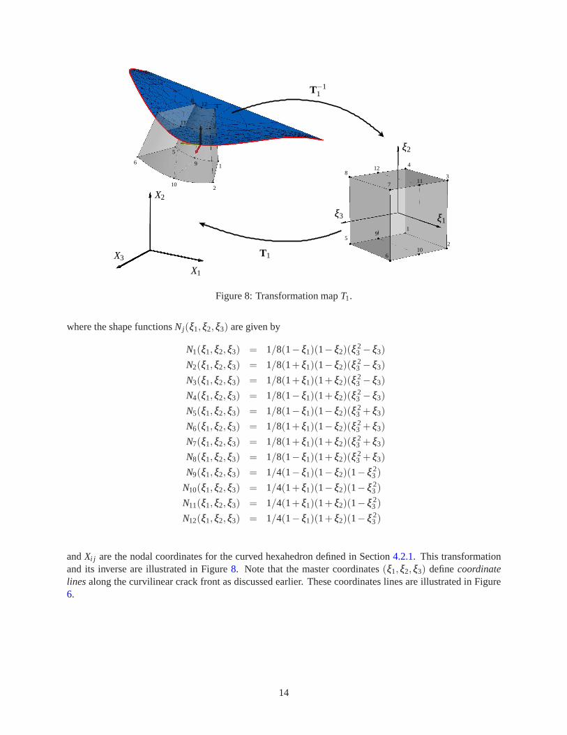
where the shape functionsNj(ξ1,ξ2,ξ3) are given by

N1(ξ1,ξ2,ξ3) = 1/8(1−ξ1)(1−ξ2)(ξ 23 −ξ3)

N2(ξ1,ξ2,ξ3) = 1/8(1+ξ1)(1−ξ2)(ξ 23 −ξ3)

N3(ξ1,ξ2,ξ3) = 1/8(1+ξ1)(1+ξ2)(ξ 23 −ξ3)

N4(ξ1,ξ2,ξ3) = 1/8(1−ξ1)(1+ξ2)(ξ 23 −ξ3)

N5(ξ1,ξ2,ξ3) = 1/8(1−ξ1)(1−ξ2)(ξ 23 +ξ3)

N6(ξ1,ξ2,ξ3) = 1/8(1+ξ1)(1−ξ2)(ξ 23 +ξ3)

N7(ξ1,ξ2,ξ3) = 1/8(1+ξ1)(1+ξ2)(ξ 23 +ξ3)

N8(ξ1,ξ2,ξ3) = 1/8(1−ξ1)(1+ξ2)(ξ 23 +ξ3)

N9(ξ1,ξ2,ξ3) = 1/4(1−ξ1)(1−ξ2)(1−ξ 23 )

N10(ξ1,ξ2,ξ3) = 1/4(1+ξ1)(1−ξ2)(1−ξ 23 )

N11(ξ1,ξ2,ξ3) = 1/4(1+ξ1)(1+ξ2)(1−ξ 23 )

N12(ξ1,ξ2,ξ3) = 1/4(1−ξ1)(1+ξ2)(1−ξ 23 )

andXi j are the nodal coordinates for the curved hexahedron defined in Section4.2.1. This transformationand its inverse are illustrated in Figure8. Note that the master coordinates(ξ1,ξ2,ξ3) definecoordinatelinesalong the curvilinear crack front as discussed earlier. These coordinates lines are illustrated in Figure6.

14

The Jacobian for this transformation is given by

[

(JJJ1)i j =∂Xi

∂ ξ j

]

=

∂X1

∂ ξ1

∂X1

∂ ξ2

∂X1

∂ ξ3∂X2

∂ ξ1

∂X2

∂ ξ2

∂X2

∂ ξ3∂X3

∂ ξ1

∂X3

∂ ξ2

∂X3

∂ ξ3

(10)

The columns ofJJJ1 define vectors tangent to the coordinate lines in physical coordinates and are given by

ggg j =∂XXX∂ ξ j

=∂Xi

∂ ξ jeeei (11)

whereeeei is a base vector of the global coordinate system. Unitary base vectors along the crack front are thengiven by

eeej =ggg j

h j(no summation onj) (12)

where thescale factorh j is given by

h j =

√

GGG j j (no summation onj) (13)

andGGG is the metric tensor defined asGGGi j = gggi · ggg j (14)

The base vectorseeej , j = 1,2,3 are the red, black and yellow arrows illustrated in Figure6. Since thecoordinate linesξ1 andξ2 are not curvilinear, the base vectorseeej , j = 1,2,3, and the other quantities definedabove are a function ofξ3 only. This simplifies the calculations as shown in AppendixA.

The inverse mappingT−1

1 : (X1,X2,X3) 7−→ (ξ1,ξ2,ξ3)

is needed for the computational implementation of the enrichment functions as discussed in Section4.2.2.It can be numerically determined using an iterative scheme such as Newton-Raphson.

After performing the inverse mapping, the closest point on the curved front toXXX is given byXXX(0,0,ξ3).Thus, the distance ofXXX to the crack front is given by

r(XXX) =‖ XXX−XXX(0,0,ξ3) ‖ (15)

This is used below to define the curvilinear cylindrical coordinate system needed for the computation ofsingular enrichment functions (2).

Curvilinear cylindrical coordinate system along crack front Having coordinates(ξ1,ξ2,ξ3) computedusing mappingT−1

1 , a curvilinear cylindrical coordinate system along the crack front can be defined throughthe following transformation

T−12 : (ξ1,ξ2,ξ3) 7−→ (r,θ ,ξ3)

15

with the relation between coordinates in both systems givenby

r =‖ XXX(ξ1,ξ2,ξ3)−XXX(0,0,ξ3) ‖θ = arctan(

ξ2

ξ1)

(16)

The Jacobian for this transformation is given by

JJJ−12 =

cos(θ ) sin(θ ) 0

−1r

sin(θ )1r

cos(θ ) 0

0 0 1

(17)

which is equal toJJJ−1a defined in (6).

Definition of enrichment functions in global coordinates TransformationsT−11 andT−1

2 can be used to

define enrichment functionsLξ jα i(r,θ ), i = 1,2, j = 1,2,3, in global coordinates.

DefineL

ξ jα i(ξ1,ξ2,ξ3) = L

ξ jα i T−1

2 (ξ1,ξ2,ξ3) i = 1,2, j = 1,2,3 (18)

Next defineL

ξ jα i(X1,X2,X3) = L

ξ jα i T−1

1 (X1,X2,X3) i = 1,2, j = 1,2,3 (19)

In the computational implementation of the singular enrichment functions, an integration point in thesupportωα of these functions is first mapped to global coordinatesXXX and then mapped to cylindrical coor-dinates using the composition ofT−1

1 andT−12 , i.e.,

T−1 = T−12 T−1

1

whereT−1 : (X1,X2,X3) 7−→ (r,θ ,ξ3)

Mapped coordinates(r,θ ,ξ3) are then used in (2) to compute the singular functions.

The displacement vectors(Lξ1α1, L

ξ2α1, L

ξ3α1) and(Lξ1

α2, Lξ2α2, L

ξ3α2) have components in the crack front coordi-

nate directionsξ1,ξ2,ξ3 and thus must be transformed to the global Cartesian system(X1,X2,X3) using thesame procedure as in Section4.1.1. This can be done using (9) with RRRb replaced byRRR1, a rotation matrixwith columns given by the base vectorseeei , i = 1,2,3, defined in (12).

5 Numerical experiments

In the numerical examples presented in this paper, crack front enrichment functions are used at nodes whosesupport intersects the crack front. More details about the selection of nodal GFEM enrichments in 3Dfracture mechanics problems can be found in, e.g, [28].

We use the Cut-off Function Method (CFM) to extract stress intensity factors from GFEM solutions.The CFM is a superconvergent extraction technique based on Betti’s reciprocity law. It is able to deliverconvergence rates for SIFs that are on par with the convergence rate of strain energy. More details about thisextraction method can be found in, e.g, [26, 27, 36, 37].

16

5.1 Half penny-shaped crack in a prism

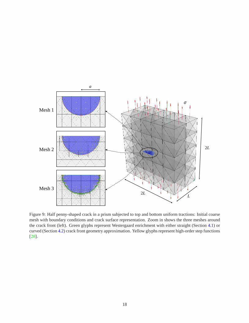
In this example, we consider a half penny-shaped crack in a prism as illustrated in Figure9. The ratio of thecharacteristic dimension,L, of the prism and the radiusa of the crack isL/a = 5.0. The prism is subjectedto top and bottom tensile tractions of magnitudeσ = 1. Figure9 illustrates the boundary conditions and thedimension of the domain of analysis. The Young’s Modulus andPoisson’s ratio are taken asE = 1.0 andν = 0.25, respectively.

The reference solution for stress intensity factor (SIF) inthis problem is provided by [39]. There, onequarter of the domain was discretized with hex-20 finite elements and appropriate symmetry boundary con-ditions applied. The localized mesh refinement around the crack front consisted of a set of seven rings ofelements. Hexagonal 20-node elements with quarter-point nodes and collapsed faces were used along thecrack front. The ratio element size to characteristic cracklength(Le/a) was 3.83×10−3 [39]. This is aroundten times smaller than the finest mesh we use (cf. Table1).

The SIF solutions(KI ) obtained in this section are normalized by the equation

KI =KI

σ√

πaQ

whereQ = 2.464 for a circular crack. More details about this normalization process can be found in [39]and references therein.

The aim of this example is to show a comparison for SIF solution between linear and quadratic crackfront geometry approximations for different mesh refinements at the crack front. Since this example has asurface breaking crack, the boundary layer effect [29] reduces the SIF values when the crack front is closeto the boundary of the domain. Because the boundary layer effect is not the main focus of this paper, wecompute the SIF in the range 10 ≤ θ ≤ 170 .

We use three GFEM meshes with different levels of refinement along the crack front and polynomial or-der of approximationp= 3. More details about high-order GFEM approximations for the class of problemsconsidered here can be found in [28]. The description of each mesh according to its level of refinement islisted in Table1. Figure9 illustrates the refinement along the crack front for the three meshes used in thisanalysis. Mesh 1 is the coarsest mesh that allows the construction of the 12-node hexahedron under theassumptions listed in Section4.2.1.

Table 1: Description of GFEM meshes used in the simulation. The ratiosLe/a listed below refer to theelements that intersect the crack front.

Le/aMesh dofs min max

1 15132 0.1250 0.31252 33102 0.0625 0.11803 82590 0.0294 0.0525

The use of coarse meshes around the crack front brings the issue of numerical integration of the singularenrichments. In [25], we show that the Keast integration rule [12] with 45 points is able to numericallyintegrate with sufficient accuracy these functions on meshes with element size typically used in the GFEM.Mesh 3 fits in this category but meshes 1 and 2 do not. In this example, we use a tensor product rule with343 points in order to control integration errors. The same rule is used on all three meshes.

17

Mesh 1

Mesh 2

Mesh 32L

L

σ

2L

a

Figure 9: Half penny-shaped crack in a prism subjected to topand bottom uniform tractions: Initial coarsemesh with boundary conditions and crack surface representation. Zoom in shows the three meshes aroundthe crack front (left). Green glyphs represent Westergaardenrichment with either straight (Section4.1) orcurved (Section4.2) crack front geometry approximation. Yellow glyphs represent high-order step functions[28].

18

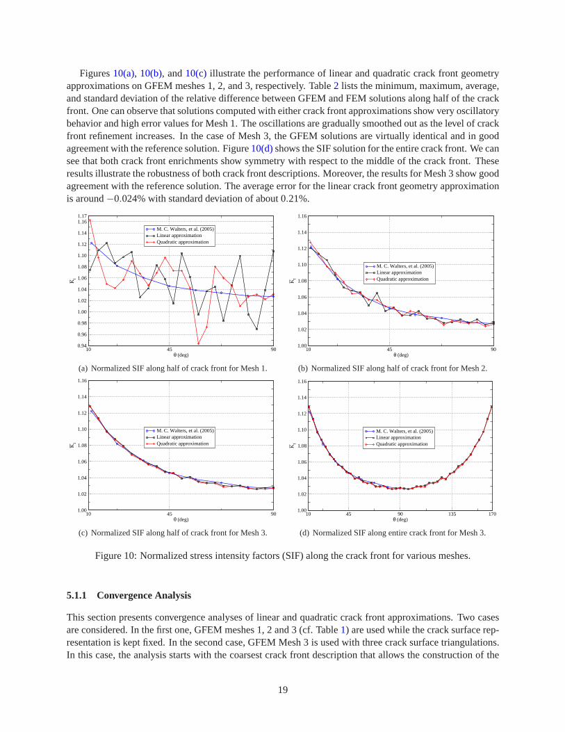
Figures10(a), 10(b), and10(c) illustrate the performance of linear and quadratic crack front geometryapproximations on GFEM meshes 1, 2, and 3, respectively. Table 2 lists the minimum, maximum, average,and standard deviation of the relative difference between GFEM and FEM solutions along half of the crackfront. One can observe that solutions computed with either crack front approximations show very oscillatorybehavior and high error values for Mesh 1. The oscillations are gradually smoothed out as the level of crackfront refinement increases. In the case of Mesh 3, the GFEM solutions are virtually identical and in goodagreement with the reference solution. Figure10(d)shows the SIF solution for the entire crack front. We cansee that both crack front enrichments show symmetry with respect to the middle of the crack front. Theseresults illustrate the robustness of both crack front descriptions. Moreover, the results for Mesh 3 show goodagreement with the reference solution. The average error for the linear crack front geometry approximationis around−0.024% with standard deviation of about 0.21%.

10 45 90θ (deg)

0.94

0.96

0.98

1.00

1.02

1.04

1.06

1.08

1.10

1.12

1.14

1.161.17

KI

M. C. Walters, et al. (2005)Linear approximationQuadratic approximation

(a) Normalized SIF along half of crack front for Mesh 1.

10 45 90θ (deg)

1.00

1.02

1.04

1.06

1.08

1.10

1.12

1.14

1.16

KI

M. C. Walters, et al. (2005)Linear approximationQuadratic approximation

(b) Normalized SIF along half of crack front for Mesh 2.

10 45 90θ (deg)

1.00

1.02

1.04

1.06

1.08

1.10

1.12

1.14

1.16

KI

M. C. Walters, et al. (2005)Linear approximationQuadratic approximation

(c) Normalized SIF along half of crack front for Mesh 3.

10 45 90 135 170θ (deg)

1.00

1.02

1.04

1.06

1.08

1.10

1.12

1.14

1.16

KI

M. C. Walters, et al. (2005)Linear approximationQuadratic approximation

(d) Normalized SIF along entire crack front for Mesh 3.

Figure 10: Normalized stress intensity factors (SIF) alongthe crack front for various meshes.

5.1.1 Convergence Analysis

This section presents convergence analyses of linear and quadratic crack front approximations. Two casesare considered. In the first one, GFEM meshes 1, 2 and 3 (cf. Table 1) are used while the crack surface rep-resentation is kept fixed. In the second case, GFEM Mesh 3 is used with three crack surface triangulations.In this case, the analysis starts with the coarsest crack front description that allows the construction of the

19

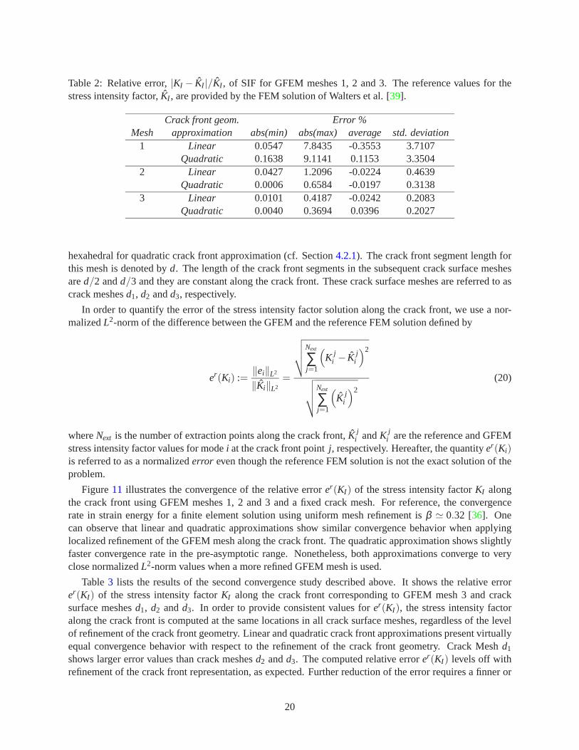
Table 2: Relative error,|KI − KI |/KI , of SIF for GFEM meshes 1, 2 and 3. The reference values for thestress intensity factor,KI , are provided by the FEM solution of Walters et al. [39].

Crack front geom. Error %Mesh approximation abs(min) abs(max) average std. deviation

1 Linear 0.0547 7.8435 -0.3553 3.7107Quadratic 0.1638 9.1141 0.1153 3.3504

2 Linear 0.0427 1.2096 -0.0224 0.4639Quadratic 0.0006 0.6584 -0.0197 0.3138

3 Linear 0.0101 0.4187 -0.0242 0.2083Quadratic 0.0040 0.3694 0.0396 0.2027

hexahedral for quadratic crack front approximation (cf. Section 4.2.1). The crack front segment length forthis mesh is denoted byd. The length of the crack front segments in the subsequent crack surface meshesared/2 andd/3 and they are constant along the crack front. These crack surface meshes are referred to ascrack meshesd1, d2 andd3, respectively.

In order to quantify the error of the stress intensity factorsolution along the crack front, we use a nor-malizedL2-norm of the difference between the GFEM and the reference FEM solution defined by

er(Ki) :=‖ei‖L2

‖Ki‖L2

=

√√√√

Next

∑j=1

(

K ji − K j

i

)2

√√√√

Next

∑j=1

(

K ji

)2

(20)

whereNext is the number of extraction points along the crack front,K ji andK j

i are the reference and GFEMstress intensity factor values for modei at the crack front pointj , respectively. Hereafter, the quantityer(Ki)is referred to as a normalizederror even though the reference FEM solution is not the exact solution of theproblem.

Figure11 illustrates the convergence of the relative errorer(KI ) of the stress intensity factorKI alongthe crack front using GFEM meshes 1, 2 and 3 and a fixed crack mesh. For reference, the convergencerate in strain energy for a finite element solution using uniform mesh refinement isβ ≃ 0.32 [36]. Onecan observe that linear and quadratic approximations show similar convergence behavior when applyinglocalized refinement of the GFEM mesh along the crack front. The quadratic approximation shows slightlyfaster convergence rate in the pre-asymptotic range. Nonetheless, both approximations converge to veryclose normalizedL2-norm values when a more refined GFEM mesh is used.

Table3 lists the results of the second convergence study describedabove. It shows the relative errorer(KI ) of the stress intensity factorKI along the crack front corresponding to GFEM mesh 3 and cracksurface meshesd1, d2 andd3. In order to provide consistent values forer(KI ), the stress intensity factoralong the crack front is computed at the same locations in allcrack surface meshes, regardless of the levelof refinement of the crack front geometry. Linear and quadratic crack front approximations present virtuallyequal convergence behavior with respect to the refinement ofthe crack front geometry. Crack Meshd1

shows larger error values than crack meshesd2 andd3. The computed relative errorer(KI ) levels off withrefinement of the crack front representation, as expected. Further reduction of the error requires a finner or

20

10000 100000Number of degrees of freedom

0.001

0.01

0.05

Nor

mal

ized

L2 -nor

m

quadratic approximationlinear approximation

βlin.

= 2.64

βlin.

= 0.86

βquad.

= 3.01

βquad.

= 0.45

Figure 11: Relative errorer(KI ) of the stress intensity factorKI along the crack front for linear and quadraticcrack front approximations.βlin. andβquad.denote the convergence rate for linear and quadratic approxima-tions, respectively. GFEM meshes 1, 2 and 3 and a fixed crack mesh are used in the computations.

higher order GFEM mesh.

Table 3: Convergence analysis of GFEM solution with respectto the refinement of the crack front descriptionfor linear and quadratic crack front approximations.

er(KI )Mesh Front segment linear quadratic

d1 d = 0.0283 0.003754 0.003832d2 d/2 = 0.0143 0.001794 0.001740d3 d/3 = 0.0095 0.001621 0.001638

5.2 Inner and outer circumferential cracks in a finite cylinder

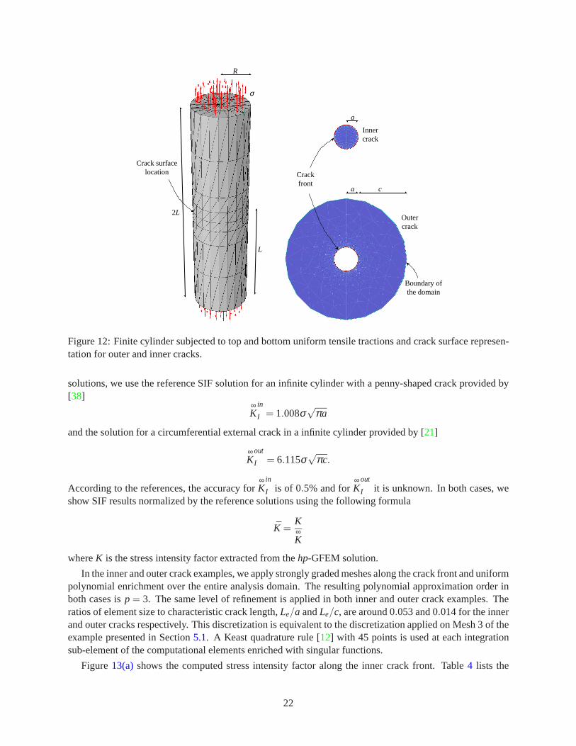
In this section, we consider two examples of cracks in a finitecylinder. The cylinder has dimensionsL/R= 4,where 2L is the height of the cylinder andR is the radius of its cross section. We set a large ratio betweenheight and radius of the cylinder in order to minimize the finite domain effect in the extraction of stressintensity factors. The model is subjected to unit tensile load σ = 1 on top and bottom faces.E = 1 andν = 0.3 are the material parameters assigned to the cylinder. The first example is a penny-shaped crack,hereafter referred to asinner crack, in the middle of the cylinder. For this exampleR/a = 5, wherea is theradius of the crack. The second example is a circumferentialsurface breaking crack, from now on referredto asouter crack, in the middle of the cylinder. In this case,a defines the material ligament. The ratio of theradius of the cylinder(R) to the crack length(c) is R/c = 1.25. The ratios cylinder radius to crack size,R/aandR/c, are set such that the inner and outer crack front geometriesare the same. Figure12 illustrates thedomain of analysis and the crack surfaces used in the simulations.

The main objective of these examples is to compare the robustness of the crack front enrichment functionsin cases where the curved crack front is convex (inner crack)and concave (outer crack). As reference

21

a c

R

L

2L

a

Crack surfacelocation

Boundary ofthe domain

Crackfront

σ

Outercrack

Innercrack

Figure 12: Finite cylinder subjected to top and bottom uniform tensile tractions and crack surface represen-tation for outer and inner cracks.

solutions, we use the reference SIF solution for an infinite cylinder with a penny-shaped crack provided by[38]

∞K

in

I = 1.008σ√

πa

and the solution for a circumferential external crack in a infinite cylinder provided by [21]

∞K

out

I = 6.115σ√

πc.

According to the references, the accuracy for∞K

in

I is of 0.5% and for∞K

out

I it is unknown. In both cases, weshow SIF results normalized by the reference solutions using the following formula

K =K∞K

whereK is the stress intensity factor extracted from thehp-GFEM solution.

In the inner and outer crack examples, we apply strongly graded meshes along the crack front and uniformpolynomial enrichment over the entire analysis domain. Theresulting polynomial approximation order inboth cases isp = 3. The same level of refinement is applied in both inner and outer crack examples. Theratios of element size to characteristic crack length,Le/a andLe/c, are around 0.053 and 0.014 for the innerand outer cracks respectively. This discretization is equivalent to the discretization applied on Mesh 3 of theexample presented in Section5.1. A Keast quadrature rule [12] with 45 points is used at each integrationsub-element of the computational elements enriched with singular functions.

Figure13(a)shows the computed stress intensity factor along the inner crack front. Table4 lists the

22

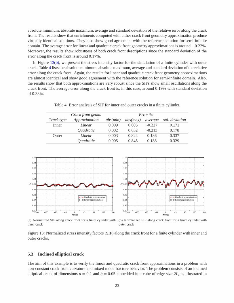
absolute minimum, absolute maximum, average and standard deviation of the relative error along the crackfront. The results show that enrichments computed with either crack front geometry approximation producevirtually identical solutions. They also show good agreement with the reference solution for semi-infinitedomain. The average error for linear and quadratic crack front geometry approximations is around−0.22%.Moreover, the results show robustness of both crack front descriptions since the standard deviation of theerror along the crack front is around 0.17%.

In Figure13(b), we present the stress intensity factor for the simulation of a finite cylinder with outercrack. Table4 lists the absolute minimum, absolute maximum, average and standard deviation of the relativeerror along the crack front. Again, the results for linear and quadratic crack front geometry approximationsare almost identical and show good agreement with the reference solution for semi-infinite domain. Also,the results show that both approximations are very robust since the SIFs show small oscillations along thecrack front. The average error along the crack front is, in this case, around 0.19% with standard deviationof 0.33%.

Table 4: Error analysis of SIF for inner and outer cracks in a finite cylinder.

Crack front geom. Error %Crack type Approximation abs(min) abs(max) average std. deviation

Inner Linear 0.009 0.605 -0.227 0.171Quadratic 0.002 0.632 -0.213 0.178

Outer Linear 0.003 0.824 0.186 0.337Quadratic 0.005 0.845 0.188 0.329

-180 -135 -90 -45 0 45 90 135 180θ (deg)

0.95

0.96

0.97

0.98

0.99

1.00

1.01

1.02

1.03

1.04

1.05

KI

Quadratic approximationLinear approximation

(a) Normalized SIF along crack front for a finite cylinder withinner crack

-180 -135 -90 -45 0 45 90 135 180θ (deg)

0.95

0.96

0.97

0.98

0.99

1.00

1.01

1.02

1.03

1.04

1.05

KI

Quadratic approximationLinear approximation

(b) Normalized SIF along crack front for a finite cylinder withouter crack

Figure 13: Normalized stress intensity factors (SIF) alongthe crack front for a finite cylinder with inner andouter cracks.

5.3 Inclined elliptical crack

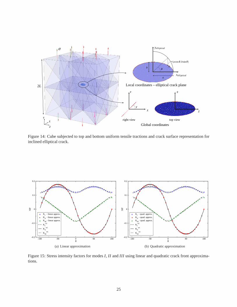
The aim of this example is to verify the linear and quadratic crack front approximations in a problem withnon-constant crack front curvature and mixed mode fracturebehavior. The problem consists of an inclinedelliptical crack of dimensionsa = 0.1 andb = 0.05 embedded in a cube of edge size 2L, as illustrated in

23

Figure14. In order to reduce the finite domain effect on the solution, we seta/L = 10. The material param-eters used in this analysis areE = 1.0×103 andν = 0.30. The slope of the crack with respect to they-axisis γ = π/4. The domain is subjected to a uniform tensile tractionσ = 1 in they-axis. Figure14 illustratesthe model and the initial coarse mesh used in this example. Inthe discretization of the solution, we applylocalized mesh refinement on GFEM elements that intersect the crack front and polynomial enrichment oforderp = 3 over the entire domain. The range of the ratio of element size along the crack front,Le, to char-acteristic crack length,a, is 0.018≤ Le/a≤ 0.041. The crack surface is represented using a quasi uniformtriangulation.

The stress intensity factors for modesI , II , andIII of an inclined elliptical crack embedded in an infinitedomain are used as reference. These SIFs are given by [38]

K inf.I =

σ sin2γ√

πbE(k)

[

sin2θ +

(ba

)2

cos2θ

] 14

K inf.II = − σ sinγ cosγ

√πbk2

[

sin2 θ +

(ba

)2

cos2 θ

] 14

[k′

Bcosω cosθ +

1C

sinω sinθ]

K inf.III =

σ sinγ cosγ√

πb(1−ν)k2

[

sin2 θ +

(ba

)2

cos2 θ

] 14

[1B

cosω sinθ − k′

Csinω cosθ

]

whereB, C, K(k) andE(k) are defined as

B = (k2−ν)E(k)+νk′2K(k), C = (k2−νk′2)E(k)−νk′2K(k),

K(k) =∫ π

2

0

dϕ√

1−k2sin2 ϕ, E(k) =

∫ π2

0

√

1−k2sin2 ϕdϕ ,

andk2 = 1−k′2, k′ = b/a andθ is a parametric angle representing a pointA on the crack front (cf. Figure14). For the example solved in this section,γ = π/4 andω = π/2.

Figure15(a)and15(b)illustrate the comparison of linear and quadratic crack front approximations withrespect to the infinite domain solution, respectively. One can note that both approximations show goodagreement with the infinite domain solution. Table5 lists the normalizedL2-norm of the difference betweenthe numerical solution and the reference solution (cf. Equation (20)). Like in the previous examples, wecan observe that both approximations provide virtually thesame results. The relative errors of the stressintensity factors along the crack front for linear and quadratic approximations show very small differences.

Table 5: NormalizedL2-norm of the error of the SIFs along the crack front for linearand quadratic approx-imations.

Crack front geom.approximation er(KI ) er(KII ) er(KIII )

Linear 0.0234 0.00406 0.04133Quadratic 0.0223 0.00486 0.04246

24

σ

2L

Z

X

Y

Z

right view

γ

X

θ

a

b

xelliptical

A

(acosθ ,bsinθ)

yelliptical

top viewX

Y

Local coordinates – elliptical crack plane

Global coordinates

Figure 14: Cube subjected to top and bottom uniform tensile tractions and crack surface representation forinclined elliptical crack.

-180 -90 0 90 180θ

-0.2

-0.1

0

0.1

0.2

SIF

KI

- linear approx.

KII

- linear approx.

KIII

- linear approx.

KI

inf.

KII

inf.

KIII

inf.

(a) Linear approximation

-180 -90 0 90 180θ

-0.2

-0.1

0

0.1

0.2

SIF

KI

- quad. approx.

KII

- quad. approx.

KIII

- quad. approx.

KI

inf.

KII

inf.

KIII

inf.

(b) Quadratic approximation

Figure 15: Stress intensity factors for modesI , II andIII using linear and quadratic crack front approxima-tions.

25

6 Concluding remarks

Linear and quadratic approximations to represent curvilinear crack fronts are presented. These represen-tations are geared towards the construction of enrichment functions for the generalized finite element. Inboth cases, special care is taken when setting the crack front coordinate system based on the geometricdescription of the crack front. The evaluation of crack front normals, tangents and conormals vectors usingmedial-quadric-based techniques ensures the robustness of the representation of the crack front geometry.

The results presented in Section5 show that a coarse mesh with either linear or quadratic crackfrontgeometry approximations leads to poor crack front description. As a result, the SIF solution along the crackfront shows poor accuracy and very oscillatory behavior. However, by applying a suitable refinement levelalong the crack front the results show that both approaches lead to the same crack front representation in thelimit case, i.e., when the crack front refinement is enough tocapture the singular solution along the crackfront.

The numerical experiments indicate that both crack front geometry approximations lead to very robustresults in meshes typically used for this class of problem. The first approach uses Cartesian coordinatesystems along the crack front and is straightforward to implement. The implementation of the secondapproach is more involved since it is based on curvilinear coordinate systems. Thus,for the class of problemsconsidered here, the first approach is recommended.

The proposed approaches to build enrichment functions along curved crack fronts are not limited tothe case of linear elastic fracture mechanics, the focus of this paper. Application of these approaches tothe case of cohesive cracks, and other non-linear fracture mechanics problems is straightforward. Thesame procedure used to define the curvilinear coordinate system along the crack front can be used. Theconclusions regarding which approach is better for other classes of problem may, of course, be differentfrom the case considered here.

Acknowledgments: The authors wish to thank Prof. Sergio Proenca from the School of Engineering atSao Carlos - University of Sao Paulo, Brazil, for fruitful discussions during the course of this research.The support of the first two authors by the University of Illinois at Urbana-Champaign is also gratefullyacknowledged.

26

A Gradient of Enrichment Functions in Global Coordinates

This section presents the computation of the gradient of enrichment functions with respect to the globalcoordinatesX1, X2, X3. These quantities, in turn, are used in the computation of derivatives of GFEM shapefunctions defined in (1).

A.1 Case 1: Linear Approximation of Crack Front Geometry

In this section, we consider the case of the derivatives of the enrichment functions defined in Section4.1.1.

Let uuu(r,θ ) denote a displacement vector with components(u1, u2, u3) whereu j equal toLξ j

α1 or Lξ j

α2, forj = 1,2,3, andα arbitrary. Similarly, we define vectorsuuu(ξ1,ξ2,ξ3) anduuu(X1,X2,X3) using enrichment

functionsLξ jα i(ξ1,ξ2,ξ3) andL

Xjα i ,(X1,X2,X3), i = 1,2, j = 1,2,3, respectively.

Let r i , i = 1,2,3, denote cylindrical coordinatesr, θ and ξ3, respectively. The gradient ofuuu can becomputed using the derivatives of the functions defined in (2) and is given by

uuu←−ξ =

∂ u j

∂ ξleeej ⊗ eeel =

∂ u j

∂ rm

∂ rm

∂ ξleeej ⊗ eeel

where, from (6),∂ rm

∂ ξl=(JJJ−1

a

)

ml

The relation between the base vectorseeem, m= 1,2,3, of a Cartesian crack front coordinate system andthe global based vectorseeei , i = 1,2,3, is given by

eeem =(RRR−1

b

)

mieeei

whereRRR−1b = JJJ−1

b (cf. Section4.1.1).

Using the above, the gradient ofuuu can be computed as follows

uuu←−ξ =

∂ um

∂ ξneeem⊗ eeen =

∂ um

∂ ξn

(RRR−1

b

)

mieeei⊗(RRR−1

b

)

n j eeej

=(RRR−1

b

)

mi

∂ um

∂ ξn

(RRR−1

b

)

n j eeei⊗eeej =∂ui

∂Xjeeei⊗eeej = uuu

←−X

Thus, the derivatives of the enrichment functions with respect to global coordinates can be computedusing

∂ui

∂Xj=(RRR−1

b

)

mi

∂ um

∂ ξn

(RRR−1

b

)

n j

In matrix form, we have [

uuu←−X

]

= RRRb

[

uuu←−ξ

]

RRRTb .

A.2 Case 2: Quadratic Approximation of Crack Front Geometry

The case of enrichment functions defined using a quadratic approximation of the crack front geometryfollows the same steps as in the section above. However, in this case, the coordinate system is curvilinear.The computation of the gradient of the displacement vector with respect to curvilinear coordinates must also

27

consider the derivatives of the crack front base vectors andscale factors. This is presented below in SectionsA.2.1 andA.2.2, respectively.

A.2.1 Derivatives of crack front base vectors

In general, the base vectors of a curvilinear system vary in length and orientation from point to point inspace. In an orthonormal system the length of the vectors is always unit, but their orientations may change.Therefore, a curvilinear orthonormal base system can be regarded as a triad that rigidly rotates from pointto pont in the curvilinear space.

The derivatives of a curvilinear orthonormal basis can be written as follows [15]

∂ eeej

∂ ξi=

[

δik

h j

∂ hi

∂ ξ j− δi j

hk

∂ h j

∂ ξk

]

eeek (21)

All sectionsξ3 = C, whereC is a constant, of the 12-node hexahedron element used in the definition ofcurvilinear coordinate systems (cf. Section4.2.1) have the following properties

• They are squared, i.e., there is no distortion on theξ1 ξ2 plane;

• all section have the same dimensions;

• they are planar, i.e. there is no warping on theξ1 ξ2 plane.

Based on these assumptions, the base vectorseeej , j = 1,2,3, are dependent onξ3 only and all scaling factorsare constant, excepth3.

Depending on the nodal coordinates of the element, however,sectionsξ3 = C may be non-orthogonal tothe coordinate lineξ3. This happens if the element has a large curvature in theξ3 direction. The procedurepresented in Section4.2.1, however, keeps this distortion to a minimum. Furthermore,even when theelement is distorted, this is much less pronounced near the centroid of the element. The enriched cloud(ωα) is located, by construction, almost at the center of the hexahedron. Therefore, it is reasonable toassume that the base vectorseeej , j = 1,2,3, form an orthonormal basis over the enriched cloud(ωα).

Based on the above, the derivatives of the base vectorseeej , j = 1,2,3, reduce to

∂ eee1

∂ ξ3=

1

h1

∂ h3

∂ ξ1eee3 (22)

∂ eee2

∂ ξ3=

1

h2

∂ h3

∂ ξ2eee3 (23)

∂ eee3

∂ ξ3= − 1

h1

∂ h3

∂ ξ1eee1−

1

h2

∂ h3

∂ ξ2eee2 (24)

and all other components are zero.

A.2.2 Derivatives of the scale factors

The derivatives the scale factors defined in (13) can be written as follows.

∂ h j

∂ ξi=

1

h j

∂ ggg j

∂ ξi· ggg j =

1

h j

∂ 2Xk

∂ ξi∂ ξ j

∂Xk

∂ ξ j(25)

28

with no summation onj .

Based on the discussion in the previous section, only the following terms are non-zero

∂ h3

∂ ξ1=

1

h3

∂ 2Xk

∂ ξ1∂ ξ3

∂Xk

∂ ξ3(26)

∂ h3

∂ ξ2=

1

h3

∂ 2Xk

∂ ξ2∂ ξ3

∂Xk

∂ ξ3. (27)

A.2.3 Gradient of the displacement field

Let uuu be a displacement vector with components given by enrichment functionsLξiαn(ξ1,ξ2,ξ3), n = 1 or

n = 2 andi = 1,2,3, as in SectionA.1. The gradient ofuuu with respect to curvilinear coordinatesξ1,ξ2,ξ3

can be computed using [30]

uuu←−ξ = u j eeej ⊗

←−∂

∂ ξieeei

1

hi= (u1eee1 + u2eee2 + u3eee3)⊗

( ←−∂

∂ ξ1eee1

1

h1+

←−∂

∂ ξ2eee2

1

h2+

←−∂

∂ ξ3eee3

1

h3

)

=1

hi

∂ u j

∂ ξieeej ⊗ eeei +

u j

hi

∂ eeej

∂ ξi⊗ eeei

(28)

In indicial notation, we have

(

uuu←−ξ

)

ki=

1

hi

(

∂ uk

∂ ξi+

u j

h j

∂ hi

∂ ξ jδik−

ui

hk

∂ hi

∂ ξk

)

Using∂ uk

∂ ξi=

∂ uk

∂ r l

∂ r l

∂ ξi, where

∂ r l

∂ ξi=(JJJ−1

2

)

li , we have

(

uuu←−ξ

)

ki=

1

hi

∂ uk

∂ r l

∂ r l

∂ ξi︸ ︷︷ ︸

derivatives of displacements

+u j

h j

∂ hi

∂ ξ jδik−

ui

hk

∂ hi

∂ ξk︸ ︷︷ ︸

derivatives of vectors

(29)

whereuk,k = 1,2,3, are the components of vectoruuu defined in SectionA.1. The indices of the scale factorsdo not take part in the summation convention.

Using the results from SectionsA.2.1 andA.2.2, we can write the components of the gradient of thedisplacement vectoruuu in matrix form

[

uuu←−ξ

]

=

1

h1

∂ u1

∂ ξ1

1

h2

∂ u1

∂ ξ2

1

h3

∂ u1

∂ ξ31

h1

∂ u2

∂ ξ1

1

h2

∂ u2

∂ ξ2

1

h3

∂ u2

∂ ξ31

h1

∂ u3

∂ ξ1

1

h2

∂ u3

∂ ξ2

1

h3

∂ u3

∂ ξ3

+

0 0 − u3

h3

1

h1

∂ h3

∂ ξ1

0 0 − u3

h3

1

h2

∂ h3

∂ ξ2

0 0u1

h1

1

h3

∂ h3

∂ ξ1+

u2

h2

1

h3

∂ h3

∂ ξ2

(30)

We can now compute the gradient of the enrichment functions with respect to global coordinates usingthe same steps as in SectionA.1.

The relation between the base vectorseeem, m= 1,2,3, of a curvilinear crack front coordinate system and

29

the global based vectorseeei , i = 1,2,3 is given by

eeem =(RRR−1

1

)

mieeei

whereRRR−11 is a rotation matrix with rows given by the base vectorseeei , i = 1,2,3, defined in Section4.2.2,

i.e.,(RRR−1

1

)

i j =1

hi

∂Xj

∂ ξi

This transformation tensor is dependent onξ3, the position along the crack front. Again, no summation isimplied over the indicei of the scale factors.

Using the above(

uuu←−X

)

i j=(RRR−1

1

)

mi

(

uuu←−ξ

)

mn

(RRR−1

1

)

n j

where(

uuu←−ξ

)

mnare the components of the gradient of the displacement vector uuu in the curvilinear system

as defined in (29) and(

uuu←−X

)

i jare the gradient components in global coordinates.

In matrix form, we have [

uuu←−X

]

= RRR1

[

uuu←−ξ

]

RRRT1 .

References

[1] I. Babuska and J.M. Melenk. The partition of unity finite element method. International Journal forNumerical Methods in Engineering, 40:727–758, 1997.1, 3

[2] T. Belytschko and T. Black. Elastic crack growth in finiteelements with minimal remeshing.Interna-tional Journal for Numerical Methods in Engineering, 45:601–620, 1999.2

[3] D.L. Chopp and N. Sukumar. Fatigue crack propagation of multiple coplanar cracks with the coupledextended finite element/fast marching method.International Journal of Engineering Science, 41:845–869, 2003.4

[4] C.A. Duarte, I. Babuska, and J.T. Oden. Generalized finite element methods for three dimensionalstructural mechanics problems.Computers and Structures, 77:215–232, 2000.1, 2, 3, 4, 10

[5] C.A. Duarte, O.N. Hamzeh, T.J. Liszka, and W.W. Tworzydlo. A generalized finite element methodfor the simulation of three-dimensional dynamic crack propagation. Computer Methods in Ap-plied Mechanics and Engineering, 190(15-17):2227–2262, 2001. http://dx.doi.org/10.1016/S0045-7825(00)00233-4.2, 3, 4

[6] C.A. Duarte, L.G. Reno, and A. Simone. A high-order generalized FEM for through-the-thicknessbranched cracks.International Journal for Numerical Methods in Engineering, 72(3):325–351, 2007.http://dx.doi.org/10.1002/nme.2012.2

[7] C.A.M. Duarte and J.T. Oden. Anhp adaptive method using clouds.Computer Methods in AppliedMechanics and Engineering, 139:237–262, 1996.2

[8] M. Duflot. A study of the representation of cracks with level sets.International Journal for NumericalMethods in Engineering, 70:1261–1302, 2007.5

30

[9] M. Fleming, Y. A. Chu, B. Moran, and T. Belytschko. Enriched element-free Galerkin methods forcrack tip fields.International Journal for Numerical Methods in Engineering, 40:1483–1504, 1997.2

[10] X. Jiao. Face offsetting: A unified framework for explicit moving interfaces.Journal of ComputationalPhysics, 220(2):612–625, 2007.6

[11] X. Jiao, N. R. Bayyana, and H. Zha. Optimizing surface triangulation via near isometry with referencemeshes. In Y. S. Geert, D. van Albada, J. Dongarra, and P. M. A.Sloot, editors,Computational Science– ICCS 2007, pages 334–341, Beijing, China, May 2007. Springer. Proceedings, Part I.6

[12] P. Keast. Moderate-degree tetrahedral quadrature formulas.Computer Methods in Applied Mechanicsand Engineering, 55:339–348, 1986.17, 22

[13] P. Lancaster and K. Salkauskas. Surfaces generated by moving least squares methods.Mathematics ofComputation, 37(155):141–158, 1981.2

[14] P. Lancaster and K. Salkauskas.Curve and Surface Fitting, an Introduction. Academic Press, SanDiego, 1986.2

[15] L.P. Lebedev and M.J. Cloud.Tensor Analysis. World Scientific, New Jersey, 2003.28

[16] J.M. Melenk and I. Babuska. The partition of unity finite element method: Basic theory and applica-tions. Computer Methods in Applied Mechanics and Engineering, 139:289–314, 1996.1, 3

[17] J. Mergheim, E. Kuhl, and P. Steinmann. A finite element method for the computational modeling ofcohesive cracks.International Journal for Numerical Methods in Engineering, 63:276–289, 2005.2

[18] N. Moes and T. Belytschko. Extended finite element method for cohesive crack growth.EngineeringFracture Mechanics, 69:813–833, 2002.2

[19] N. Moes, J. Dolbow, and T. Belytschko. A finite element method for crack growth without remeshing.International Journal for Numerical Methods in Engineering, 46:131–150, 1999.2

[20] N. Moes, A. Gravouil, and T. Belytschko. Non-planar 3D crack growth by the extended finite el-ement and level sets – Part I: Mechanical model.International Journal for Numerical Methods inEngineering, 53(11):2549–2568, 2002.2, 4, 5

[21] Y. Murakami.Stress intensity factors handbook, volume 3. Pergamon, Oxford, New York, 1st edition,1992.22

[22] J.T. Oden and C.A. Duarte. Chapter: Clouds, Cracks and FEM’s. In B.D. Reddy, editor,RecentDevelopments in Computational and Applied Mechanics, pages 302–321, Barcelona, Spain, 1997.International Center for Numerical Methods in Engineering, CIMNE. 2, 3, 4

[23] J.T. Oden, C.A. Duarte, and O.C. Zienkiewicz. A new cloud-basedhpfinite element method.ComputerMethods in Applied Mechanics and Engineering, 153:117–126, 1998.1, 3

[24] J.T. Oden and C.A.M. Duarte. Chapter: Solution of singular problems usinghp clouds. In J.R.Whiteman, editor,The Mathematics of Finite Elements and Applications– Highlights 1996, pages 35–54, New York, NY, 1997. John Wiley & Sons.2, 3, 4

[25] K. Park, J.P. Pereira, C.A. Duarte, and G.H. Paulino. Integration of singular enrichment functions inthe generalized/extended finite element method for three-dimensional problems.International Journalfor Numerical Methods in Engineering, 2008. Accepted for publication.4, 17

31

[26] J.P. Pereira and C.A. Duarte. Computation of stress intensity factors for pressurized cracks usingthe generalized finite element method and superconvergent extraction techniques. In P.R.M. Lyra,S.M.B.A. da Silva, F.S. Magnani, L.J. do N. Guimaraes, L.M. da Costa, and E. Parente Junior, editors,XXV Iberian Latin-American Congress on Computational Methods in Engineering, Recife, PE, Brazil,November 2004. 15 pages. ISBN Proceedings CD: 857 409 869-8.16

[27] J.P. Pereira and C.A. Duarte. Extraction of stress intensity factors from generalized finite elementsolutions.Engineering Analysis with Boundary Elements, 29:397–413, 2005.16

[28] J.P. Pereira, C.A. Duarte, D. Guoy, and X. Jiao.Hp-Generalized FEM and crack surface representa-tion for non-planar 3-D cracks.International Journal for Numerical Methods in Engineering, 2008.http://dx.doi.org/10.1002/nme.2419.2, 3, 4, 5, 10, 16, 17, 18

[29] J.C. Raju, I.S. Newman Jr. Stress-intensity factors for a wide range of semi-elliptical surface cracks infinite-thickness plates.Engineering Fracture Mechanics, 11:817–829, 1979.17

[30] J.N. Reddy and M.L. Rasmussen.Advanced Engineering Analysis. John Wiley and Sons, New York,1982.29

[31] A. Simone. Partition of unity-based discontinuous elements for interface phenomena: Computationalissues.Communications in Numerical Methods in Engineering, 20:465–478, 2004.2

[32] A. Simone, G.N. Wells, and L.J. Sluys. From continuous to discontinuous failure in a gradient-enhanced continuum damage model.Computer Methods in Applied Mechanics and Engineering,192(41-42):4581–4607, 2003.2

[33] T. Strouboulis, K. Copps, and I. Babuska. The generalized finite element method.Computer Methodsin Applied Mechanics and Engineering, 190:4081–4193, 2001.1, 3

[34] N. Sukumar, D.L. Chopp, and B. Moran. Extended finite element method and fast marching methodfor three-dimensional fatigue crack propagation.Engineering Fracture Mechanics, 70:29–48, 2003.4,5

[35] N. Sukumar, N. Moes, B. Moran, and T. Belytschko. Extended finite element method forthree-dimensional crack modelling.International Journal for Numerical Methods in Engineering,48(11):1549–1570, 2000.2, 4, 5

[36] B. Szabo and I. Babuska.Finite Element Analysis. John Wiley and Sons, New York, 1991.4, 16, 20

[37] B. A. Szabo and I. Babuska. Computation of the amplitude of stress singular terms for cracks andreentrant corners. In T.A. Cruse, editor,Fracture Mechanics: Nineteenth Symposium, ASTM STP 969,pages 101–124, Southwest Research Institute, San Antonio,TX, 1988.16

[38] H. Tada, P. Paris, and G. Irwin.The Stress Analysis of Cracks Handbook. ASME Press, New York, 3rdedition, 2000.22, 24

[39] M. C. Walters, G. H. Paulino, and R. H. Dodds Jr. Stress-intensity factors for surface cracks in func-tionally graded materials under mode-I thermomechanical loading.International Journal of Solids andStructures, 41:1081–1118, 2004.17, 20

[40] G.N. Wells, R. de Borst, and L.J. Sluys. A consistent geometrically non-linear approach for delamina-tion. International Journal for Numerical Methods in Engineering, 54:1333–1355, 2002.2

32

[41] G.N. Wells and L.J. Sluys. A new method for modeling cohesive cracks using finite elements.Inter-national Journal for Numerical Methods in Engineering, 50:2667–2682, 2001.2

[42] G. Zi and T. Belytschko. New crack-tip elements for XFEMand applications to cohesive cracks.International Journal for Numerical Methods in Engineering, 57:2221–2240, 2003.2

33