Generalized ®nite element methods for three-dimensionalstructural mechanics problems

C.A. Duartea,*, I. BabusÏ kab, J.T. OdenaCOMCO, Inc., 7800 Shoal Creek Blvd. Suite 290E, Austin, TX 78757, USA

bTICAM, The University of Texas at Austin, SHC 310, Austin, TX 78712, USA

Received 26 February 1999; accepted 23 August 1999

Abstract

The present paper summarizes the generalized ®nite element method formulation and demonstrates some of itsadvantages over traditional ®nite element methods to solve complex, three-dimensional (3D) structural mechanicsproblems. The structure of the sti�ness matrix in the GFEM is compared to the corresponding FEM matrix. The

performance of the GFEM and FEM in the solution of a 3D elasticity problem is also compared. The constructionof p-orthotropic approximations on tetrahedral meshes and the use of a-priori knowledge about the solution ofelasticity equations in three-dimensions are also presented. 7 2000 Elsevier Science Ltd. All rights reserved.

1. Introduction

The analysis of complex three-dimensional (3D)structural components has become a common task inrecent years in several manufacturing industries. How-

ever, the analysis of this class of problems using tra-ditional ®nite element methods still poses severaldi�culties. It is a common practice to use automatictetrahedral mesh generators to discretize complex 3D

structural components. This type of mesh generatorscan handle very complex geometries with a minimumof human intervention (as compared to, e.g., the man-

ual generation of a mesh of hexahedral elements). Themain drawbacks of any automatic mesh generatorsare:

1. The need of an excessive number of elements inorder to keep the aspect ratios of the ®nite elements

within reasonable bounds. This is specially true

when the component has transition zones from

bulky to slender parts.

2. Polynomial approximations, as used in traditional

®nite element methods, require the use of a large

number of elements in order to capture stress con-

centrations and singularities at corners and edges of

the domain. Meshes that are insu�ciently re®ned at

these regions are often used in order to keep the

number of degrees of freedom (dof) below a reason-

able level or simply because the available mesh gen-

erators can not create an appropriate mesh where

needed without creating an excessive number of el-

ements everywhere. This practice may lead to results

of poor quality even at points in the domain distant

from the singularities, due to numerical pollution.

3. Another drawback of automatic mesh generators,

especially when tetrahedral elements are used, is

that they preclude the use of p anisotropic approxi-

mations, that is, approximations that have di�erent

polynomial orders associated with each direction.

Problems where boundary layers occur, such as in

Computers and Structures 77 (2000) 215±232

0045-7949/00/$ - see front matter 7 2000 Elsevier Science Ltd. All rights reserved.

PII: S0045-7949(99 )00211-4

www.elsevier.com/locate/compstruc

* Corresponding author. Tel.: +1-512-467-0618; Fax: +1-

512-467-1382.

E-mail address: armando@comco.com (C.A. Duarte).

the analysis of orthotropic materials or when one of

the dimensions of the structural part is much smal-

ler than the others, are examples in which p-ortho-

tropic approximations may lead to considerable

savings in the number of dof needed to achieve

acceptable accuracy.

The generalized ®nite element method (GFEM) was

proposed independently by BabusÏ ka and colleagues

[2,3,21] (under the names `special ®nite element

methods', `generalized ®nite element method' and

`®nite element partition of unity method') and by

Duarte and Oden [9±12,25] (under the names `hp

clouds' and `cloud-based hp ®nite element method').

Several of the so-called meshless methods proposed in

recent years can also be viewed as special cases of the

generalized ®nite element method. Recent surveys on

meshless methods can be found in [6,8]. The key fea-

ture of these methods is the use of a partition of unity

(PU), which is a set of functions whose values sum to

the unity at each point x in a domain O: The analysis

of the performance and computational cost of hp

clouds, element free Galerkin [7], di�use element [22]

and reproducing kernel particle [18] methods can be

found in [12]. It was found in that study that the inte-

gration of the sti�ness matrix in these methods can be

considerably more expensive than in traditional hp

®nite element methods, depending on the choice of the

partition of unity, the Moving Least Squares PU [17],

being among the most expensive.

The present paper summarizes the ideas behind the

GFEM formulation and demonstrates through numeri-

cal examples some of the advantages of GFEM over

traditional FEM for solving complex, 3D structural

mechanics problems. In Section 5, the structure of the

sti�ness matrix in the GFEM is compared to the corre-

sponding FEM matrix. In Section 6, we compare the

performance of the GFEM and FEM in the solutionof a representative 3D elasticity problem. The use of p-

orthotropic approximations on tetrahedral meshes andthe use of a-priori knowledge about the solution of theelasticity equations in three-dimensions is also demon-

strated in that section. Finally, in Section 7, majorconclusions of the study are given.

2. Formulation of generalized ®nite element methods

In this section, we review the basic ideas behind theconstruction of generalized ®nite element approxi-mations in a one-dimensional (1D) setting using a 1D

linear ®nite element partition of unity. In Section 2.1,the GFE formulation in an n-dimensional setting ispresented. In Sections 5 and 6, we use generalized tet-

rahedral ®nite elements to discretize 3D problems. Fora more detailed discussion on the theoretical aspects ofGFE approximations, see Refs. [3,10,21,25] and the

references therein.Let u be a function de®ned on a domain O � R:

Suppose that we build an open covering

TN � foa gNa�1 �O �[Na�1

oa

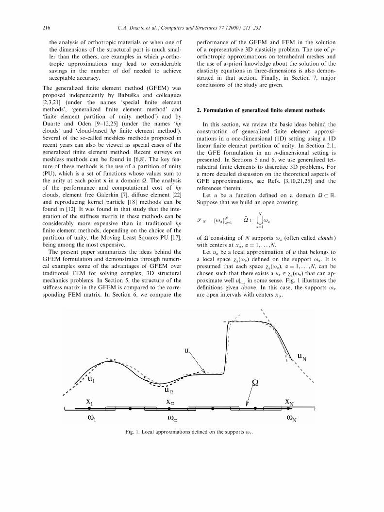
of O consisting of N supports oa (often called clouds )with centers at x a, a � 1, . . . ,N:Let ua be a local approximation of u that belongs to

a local space wa�oa� de®ned on the support oa: It ispresumed that each space wa�oa�, a � 1, . . . ,N, can bechosen such that there exists a ua 2 wa�oa� that can ap-proximate well ujoa

in some sense. Fig. 1 illustrates the

de®nitions given above. In this case, the supports oa

are open intervals with centers x a:

Fig. 1. Local approximations de®ned on the supports oa:

C.A. Duarte et al. / Computers and Structures 77 (2000) 215±232216

The local approximations ua, a � 1, . . . ,N, have tobe somehow combined together to give a global ap-

proximation uhp of u. This global approximation hasto be built such that the di�erence between uhp and u,in a given norm, be bounded by the local errors uÿua: In partition of unity methods, this is accomplishedusing functions de®ned on the supports oa,a � 1, . . . ,N, and having the following property

ja 2 C s0�oa �, sr0, 1RaRN

Xa

ja�x� � 1 8x 2 O

The functions ja are called a partition of unity subordi-

nate to the open covering TN: Examples of partitionsof unity are Lagrangian ®nite elements, the various`reproducing' functions generated by moving least

squares methods and Shepard functions [11,17].In the case of ®nite element partitions of unity, the

supports (clouds) oa are simply the union of the ®nite

elements sharing a vertex node x a (see, for exampleRefs. [21,25]). In this case, the implementation of themethod is essentially the same as in standard ®nite el-ement codes, the main di�erence being the de®nition

of the shape functions as explained below. This choiceof partition of unity avoids the problem of integrationassociated with the use of moving least squares

methods or Shepard partitions of unity used in severalmeshless methods. Here, the integrations are per-formed with the aid of the so called master elements,

as in classical ®nite elements. Therefore, the GFEMcan use existing infrastructure and algorithms devel-oped for the classical ®nite element method.

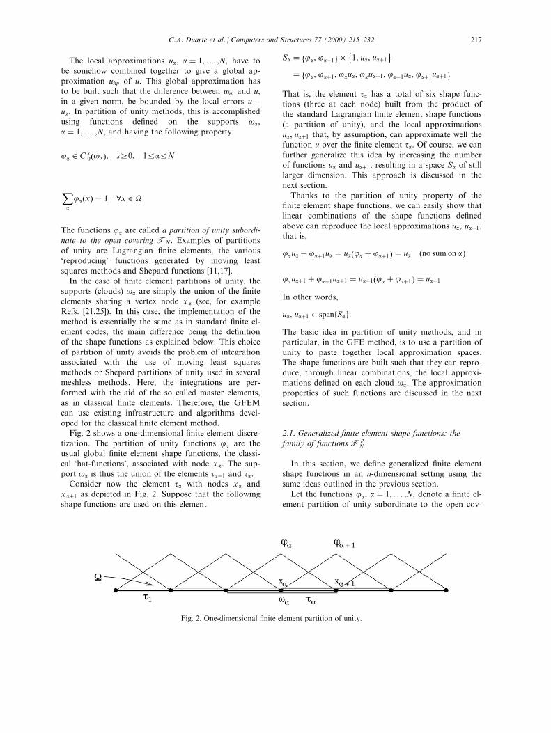
Fig. 2 shows a one-dimensional ®nite element discre-tization. The partition of unity functions ja are theusual global ®nite element shape functions, the classi-cal `hat-functions', associated with node x a: The sup-

port oa is thus the union of the elements taÿ1 and ta:Consider now the element ta with nodes x a and

x a�1 as depicted in Fig. 2. Suppose that the following

shape functions are used on this element

Sa � fja, jaÿ1 g ��1, ua, ua�1

� fja, ja�1, jaua, jaua�1, ja�1ua, ja�1ua�1 g

That is, the element ta has a total of six shape func-tions (three at each node) built from the product ofthe standard Lagrangian ®nite element shape functions

(a partition of unity), and the local approximationsua, ua�1 that, by assumption, can approximate well thefunction u over the ®nite element ta: Of course, we canfurther generalize this idea by increasing the number

of functions ua and ua�1, resulting in a space Sa of stilllarger dimension. This approach is discussed in thenext section.

Thanks to the partition of unity property of the®nite element shape functions, we can easily show thatlinear combinations of the shape functions de®ned

above can reproduce the local approximations ua, ua�1,that is,

jaua � ja�1ua � ua�ja � ja�1 � � ua �no sum on a�

jaua�1 � ja�1ua�1 � ua�1�ja � ja�1 � � ua�1

In other words,

ua, ua�1 2 spanfSa g:The basic idea in partition of unity methods, and inparticular, in the GFE method, is to use a partition of

unity to paste together local approximation spaces.The shape functions are built such that they can repro-duce, through linear combinations, the local approxi-

mations de®ned on each cloud oa: The approximationproperties of such functions are discussed in the nextsection.

2.1. Generalized ®nite element shape functions: thefamily of functions F p

N

In this section, we de®ne generalized ®nite element

shape functions in an n-dimensional setting using thesame ideas outlined in the previous section.Let the functions ja, a � 1, . . . ,N, denote a ®nite el-

ement partition of unity subordinate to the open cov-

Fig. 2. One-dimensional ®nite element partition of unity.

C.A. Duarte et al. / Computers and Structures 77 (2000) 215±232 217

ering TN � foagNa�1 of a domain O � Rn, n = 1, 2, 3.Here, N is the number of vertex nodes in the ®nite el-

ement mesh. The cloud oa is the union of the ®nite el-ements sharing the vertex node xa:Let wa�oa� � spanfLiagi2I�a� denote local spaces

de®ned on oa, a � 1, . . . ,N, where I�a�, a � 1, . . . ,N,are index sets and Lia denotes local approximationfunctions analogous with the functions ua mentioned

in the previous section. Possible choices for these func-tions are discussed below.Suppose that the ®nite element shape functions, ja,

are linear functions and that

Ppÿ1�oa � � wa�oa � a � 1, . . . ,N,

where Ppÿ1 denotes the space of polynomials of degree

less or equal to pÿ 1: The generalized ®nite elementshape functions of degree p are de®ned by [21,25]

F pN �

�fai � jaLia, a � 1, . . . ,N, i 2 I�a� �1�

Note that there is considerable freedom in the choiceof the local spaces wa: The most obvious choice for abasis of wa is polynomial functions which can approxi-

mate well smooth functions. In this case, the GFEM isessentially identical to the classical FEM. The im-plementation of hp adaptivity is, however, greatly sim-

pli®ed by the PU framework. Since each basisfunctions, fLiagi2I�a�, a � 1, . . . ,N, can have a di�erentpolynomial order for each a, we can have di�erent

polynomial orders associated with each vertex node ofthe ®nite element mesh [25]. The approximations canalso be non-isotropic (i.e., di�erent polynomial orders

in di�erent directions), regardless of the choice of ®niteelement partition of unity (hexahedral, tetrahedral,etc.). Examples of p-orthotropic approximations builton a tetrahedral mesh are given in Section 6. The con-

cept of edge and middle nodes, which is used in con-ventional p FEMs, is not needed in the framework ofGFEM. The implementation of h adaptivity is also

simpli®ed in PU methods since it needs to be doneonly on the partition of unity (linear ®nite elements inthis case). Therefore, the implementation of h adaptiv-

ity for high-order approximations is the same as forlinear approximations (there is no need, for example,of using high-order constraints as done in traditionalhp ®nite element methods).

There are many situations in which the solution of aboundary value problem is not a smooth function. Inthese situations, the use of polynomials to build the

approximation space, as in the FEM, may be far fromoptimal and may lead to poor approximations of thesolution u unless carefully designed meshes are used.

In the GFEM, we can use any a-priori knowledgeabout the solution to make better choices for the localspaces wa: For example, in Section 6, we solve a

boundary value problem in which the solution pos-sesses point or lines of singularities at some parts of

the domain. Then we can use the local spaces wa tobuild generalized ®nite element shape functions thatrepresent these singularities much more e�ectively than

polynomial functions. The construction of these custo-mized shape functions is discussed in details in Section4.

Detailed convergence analysis of the generalized®nite element method can be found in [11,12,20,21].Several a-priori error estimates along with numerical

experiments demonstrating their accuracy can also befound in those works. Below, we summarize the maina-priori error estimate for the generalized ®nite elementmethod.

Suppose that the partitions of O into ®nite elementswhich form the partition of unity satisfy the usualregularity assumptions in two and three dimensions,

and, in one dimension, the ratio between the lengths ofneighboring elements is bounded. We denote

ha � diam�oa �

h � maxa�1,...,N

ha

and

Xhp � span�fai

, a � 1, . . . ,N, i 2 I�a�

where the GFE shape functions fai are de®ned in Eq.

(1). In addition, suppose the unity function, 1, belongsto the set of local approximation functions, i.e.,

1 2 wa�oa � a � 1, . . . ,N,

and that there exists a quantity E depending of a, h, p,and u, such that

kuÿ uakE�O\oa �RE�a, h, p, u� a � 1, . . . ,N

Then, it can be proved that [11,21] 9 uhp 2 Xhp suchthat

kuÿ uhpkE�O�RC

0@XN�h�a�1

E2�a, h, p, u�1A1=2

where the constant C is independent of u, h, p.

3. Quadratic GFE shape functions for tetrahedral

elements

In this section, quadratic GFE shape functions fortetrahedral elements are de®ned and analyzed. Theissue of linear dependence of GFE shape function and

C.A. Duarte et al. / Computers and Structures 77 (2000) 215±232218

how to solve the resulting positive semi-de®nite systemof equations are also discussed.

Quadratic GFE shape functions for tetrahedral el-ements are built from the product of trilinear tetrahe-dral shape functions and linear monomials as follows

ja ��1,

xÿ x a

ha,yÿ yaha

,zÿ zaha

�a � 1, . . . ,N �2�

where ja, a � 1, . . . ,N, are standard trilinear Lagran-

gian tetrahedral shape functions (e.g., Refs. [4,5,32]),xa��x a, ya, za� are the coordinates of the node a, ha isthe diameter of the largest ®nite element sharing thenode a and N is the number of nodes in the mesh.

This transformation is used to minimize round-o�errors. For details see, for example, Refs. [10,11].In the notation of Section 2.1 we have

wa � spanfLia g � span

�1,

xÿ x a

ha,yÿ yaha

,zÿ zaha

�a � 1, . . . ,N

Consider now the case of a tetrahedral element t with,for example, nodes x1, x2, x3, x4: Then the GFE quad-

ratic shape functions for this element are given by

St � ja ��1,

xÿ x a

ha,yÿ yaha

,zÿ zaha

�a � 1, 2, 3, 4

Each quadratic tetrahedral element has therefore six-

teen shape functions (instead of ten as in classicalFEMs). It should be noted that all shape functions areassociated with the vertices of the element as in a lin-

ear element and there is no need for the concept of anedge, face or interior node, as in classical high ordertri-dimensional ®nite elements. Also, the support

(cloud) of the higher order shape functions (i.e., thedomain on which the function is non-zero) is identicalto the support of the trilinear shape functions fj1, j2,j3, j4g: This fact, as we demonstrate in Section 5, has

important implications on the structure of the sti�nessmatrix.Generalized tetrahedral shape functions that can

reproduce quadratic polynomials can also be built asfollows. Suppose that the following basis is used forthe local spaces wa, a � 1, 2, 3, 4

wa � span�1, x2, xZ, xz, Z2, Zz, z2

, a � 1, 2, 3, 4

where x � �xÿ x a�=ha, Z � �yÿ ya�=ha, z � �zÿ za�=ha:Then the shape functions for an element t with nodesx1, x2, x3, x4, are given by

~St � ja ��1, x2, xZ, xz, Z2, Zz, z2

, a � 1, 2, 3, 4

Note that we excluded from the basis of wa the el-ements x, Z, z since they can be reproduced by the par-

tition of unity functions ja, a � 1, 2, 3, 4: However, aswe demonstrate below, this is not su�cient to avoid

linear dependencies.

Theorem 1. Let St and ~St be as de®ned above. Then

(i)

spanfSt g � span�1, x, y, z, x 2, xy, xz, y2, yz, z2

� P2

(ii)

span�

~St

� span

�1, x, y, z, x 2, xy, xz, y2, yz,

z2,x 3,x 2y,x 2z,y3, y2x, y2z, z3, z2x, z2y, xyz� P3

Proof. In order to simplify the notation, we consider

here the case in which the basis functions, Lia, of waare given by {1, x, y, z }. Therefore, in this case,

St � ja ��1, x, y, z

a � 1, 2, 3, 4

Since ja, a � 1, 2, 3, 4, are trilinear tetrahedral shape

functions, there exist constants axa , aya , a

za, a � 1, 2, 3,

4, such that 8x 2 t,X4a�1

ja�x� � 1 �3�

X4a�1

axaja�x� � x �4�

X4a�1

a ya ja�x� � y �5�

X4a�1

azaja�x� � z �6�

Therefore�1, x, y, z

� spanfSt g

From the equations above we have

X4a�1

axa�jax� � xX4a�1

axaja � x 2

X4a�1

a ya �jax� � x

X4a�1

a ya ja � xy �7�

and similarly for the terms xz, y2, yz, z2: Therefore

C.A. Duarte et al. / Computers and Structures 77 (2000) 215±232 219

P2 � spanfSt g �8�

Let us now show that St is a linear dependent set and

that the rank de®ciency of St is equal to 6. Using thepartition of unity property (3) of the functions ja

X4a�1�jax� � x

X4a�1

ja � x

Using Eq. (4) and the above

X4a�1�jax� ÿ

X4a�1

axaja � 0

and similarly for the terms y and z. Therefore, thedimension of a basis of spanfStg is less or equal to 13.But

X4a�1

axa�jay� � yX4a�1

axaja � yx

Using Eq. (7) and the above

X4a�1

a ya �jax� ÿ

X4a�1

axa�jay� � 0

and similarly for the terms zx and zy. Therefore, thedimension of a basis of spanfStg is less or equal to 10.But from Eq. (8) the dimension of this set is greater or

equal to 10. This proves (i). The proof of (ii) followsthe same steps.

The linear dependencies that appear above are aconsequence of the fact that both, the partition ofunity and the basis of the local spaces wa, are poly-

nomial functions. BabusÏ ka and colleagues [15,29] haveproposed two approaches to solve the system ofequations

ÄKÄu � Äf �9�

where ÄK is a positive semi-de®nite sti�ness matrix builtfrom generalized ®nite element shape functions. The®rst approach consists simply of using a direct solverfor symmetric inde®nite systems like Refs. [13,28].

Similar implementations are presently used in severalcommercial FEM solvers. The second approach con-sists of the following iterative algorithm [15,19,29]:

Let

K � T ÄKT

u � Tÿ1 Äu

f � TÄf

where

Ti, j � di, j��������~Ki, j

qThen

Ku � f �10�The above transformation leads to a sti�ness matrixwhose diagonal entries are equal to 1. This scaledmatrix is then perturbed as follows

KE � K� EI, E > 0, Ii, j � di, j

The matrix KE is positive de®nite and hence non-singu-lar. The solution u to the system (10) is then computedusing the following sequence:

u0 � Kÿ1E f

r0 � f ÿKu0

Let e0 � uÿ u0 then

KEe0 ' Ke0 � KuÿKu0 � r0

therefore

e0 � Kÿ1E r0

Compute

ri � e0 ÿXiÿ1j�0

Kej

ei � Kÿ1E ri

ui � u0 �Xiÿ1j�0

ej

for ir1 until���� eiKei

uiKui

����is su�ciently small. Numerical experiments performedby Strouboulis et al. [15,29] show that in practice, withE � 10ÿ10, a single iteration is su�cient when using

double precision accuracy. Each iteration involves amatrix±vector multiplication, a forward- and back-sub-stitutions and lower order operations. Therefore, the

C.A. Duarte et al. / Computers and Structures 77 (2000) 215±232220

computational cost of each iteration is negligible whencompared to the factorization of the sti�ness matrix.

The solution to the original system (9) is then given by

Äu � Tu

4. Customized shape functions for an edge in 3D

There are many classes of problems for which thestructure of the underlying partial di�erential equation

can be exploited. Oden and Duarte [24,26] havedemonstrated how knowledge of the solution of theelasticity equations near a corner in 2D space can be

used in a partition of unity method to e�ciently modelthe singularities that occur in this class of problems.This type of singularity is resolved very poorly bypolynomial functions such as are used in traditional

®nite element methods, unless a very re®ned mesh isused. In this section, the formulation proposed byOden and Duarte [24,26] is extended to the case of

edges in 3D problems. Numerical examples are pre-sented in Section 6.Consider an straight edge in 3D space as depicted in

Fig. 3. In the ®gure, 2pÿ a is the opening angle. As-sociated with the edge, there is a Cartesian local coor-dinate system �x, Z, z� and a cylindrical coordinatesystem �r, y, z 0� with origins at �Ox, Oy, Oz).

The displacement ®eld u�r, y, z 0 � in the neighbor-hood of the edge (for points far from its vertices) canbe written as [30,31]

uÿr, y, z 0

��8<: ux�r, y�uZ�r, y�uz�r, y�

9=;�X1j�1

2664A�1�j

8>><>>:u�1�xj �r, y�u�1�Zj �r, y�0

9>>=>>;� A

�2�j

8>><>>:u�2�xj �r, y�u�2�Zj �r, y�0

9>>=>>;� A�3�j

8><>:00u�3�zj �r, y�

9>=>;3775 �11�

where �r, y, z 0� are the cilyndrical coordinates relatives

to the system shown in Fig. 3, ux�r, y�, uZ�r, y� anduz�r, y� are Cartesian components of u in the x-, Z- andz-directions, respectively.Assuming that the boundary is traction-free and

neglecting body forces, the functions u�1�xj , u

�1�Zj , u

�2�xj , u

�2�Zj

are given by [30,31]

uxjj�1��r, y� � rl

�1 �j

2G

nhkÿQ

�1�j

�l�1�j � 1

�icos l�1�j y

ÿ l�1�j cos�l�1�j ÿ 2

�yo

u�2�xj �r, y� �

rl�2 �j

2G

nhkÿQ

�2�j

�l�2�j � 1

�isin l�2�j y

ÿ l�2�j sin�l�2�j ÿ 2

�yo

u�1�Zj �r, y� �rl�1 �j

2G

nhk�Q�1�j

�l�1�j � 1

�isin l�1�j y

� l�1�j sin�l�1�j ÿ 2

�yo

u�2�Zj �r, y� � ÿrl�2 �j

2G

nhk�Q�2�j

�l�2�j � 1

�icos l�2�j y

� l�2�j cos�l�2�j ÿ 2

�yo

where the eigenvalues l�1�j , l�2�j are found by solving

sin l�1�j a� l�1�j sin a � 0

sin l�2�j aÿ l�2�j sin a � 0Fig. 3. Coordinate systems associated with an edge in 3D

space.

C.A. Duarte et al. / Computers and Structures 77 (2000) 215±232 221

In the case of a crack, where a � 2p, the eigenvaluesare l�1�j � l�2�j � lj

l1 � 1

2, lj � j� 1

2jr2

For the edges in the mechanical part analyzed Section6, where a = 4.525 264 2,

l�1�1 � 0:564 349 993 512 569

l�2�1 � 0:985 954 537 708 805

The material constant k and G are

k � 3ÿ 4n G � E

2�1� n�

where E is the Young's modulus and n is the Poisson'sratio. This assumes a state of plane strain which is a

good approximation for the stress state in the neigh-borhood of a straight edge in three-dimensions. Forpoints close to the vertex of the edge the stress state is

more complex (see for example Refs. [14,23]).The parameters Q

�1�j and Q

�2�j are given by

Q�1�j � ÿ

cos�l�1�j ÿ 1

�a=2

cos�l�1�j � 1

�a=2� ÿL�1�j

sin�l�1�j ÿ 1

�a=2

sin�l�1�j � 1

�a=2

Q�2�j � ÿ

sin�l�2�j ÿ 1

�a=2

sin�l�2�j � 1

�a=2� ÿL�2�j

cos�l�2�j ÿ 1

�a=2

cos�l�2�j � 1

�a=2

where

L�s�j �l�s�j ÿ 1

l�s�j � 1s � 1, 2

In the case of a crack,

Q�1�j �

�ÿ1 j � 3, 5, 7, . . .ÿL�1�j j � 1, 2, 4, 6, . . .

Q�2�j �

�ÿ1 j � 1, 2, 4, 6, . . .ÿL�2�j j � 3, 5, 7, . . .

For the edges in the mechanical part analyzed in Sec-tion 6,

Q�1�1 � 0:599 081 789 Q�2�2 � ÿ0:032 551 169

The functions u�3�zj are given by Ref. [30] (assuming that

the boundary is traction-free and neglecting bodyforces)

u�3�zj �

8>>>><>>>>:rl�3 �j

2Gsin l�3�j y j � 1, 3, 5, . . .

rl�3 �j

2Gcos l�3�j y j � 2, 4, 6, . . .

where

l�3�j �jpa

j � 1, 2, . . .

Before using the above functions to build customized

GFE shape functions, they have ®rst to be transformedto the physical coordinates (x, y, z ) as follows:De®ne

u�s�xj �x, Z, z� � u�s�xj � Tÿ11 �x, Z, z�u�s�Zj �x, Z, z� � u

�s�Zj � Tÿ11 �x, Z, z�

u�3�zj �x, Z, z� � u�s�zj � Tÿ11 �x, Z, z�

s � 1, 2 j � 1, . . . ,M

Tÿ11 :�x, Z, z�4ÿr, y, z 0

��12�

8<: ryz 0

9=; �8>>>>><>>>>>:

���������������x2 � Z2

qarctan

�Zx

�z

9>>>>>=>>>>>;�13�

The coordinate system �x, Z, z� is shown in Fig. 3.

Next de®ne

~u�s�xj �x, y, z� � u

�s�xj � Tÿ12 �x, y, z�

~u�s�Zj �x, y, z� � u�s�Zj � Tÿ12 �x, y, z�~u�3�zj �x, y, z� � u

�3�Zj � Tÿ12 �x, y, z�

s � 1, 2 j � 1, . . . ,M

Tÿ12 :�x, y, z�4 �x, Z, z� �14�

8<: xZz

9=; � Rÿ12

8<: xÿOx

yÿOy

zÿOz

9=; �15�

where Rÿ12 2 R3 � R3, with rows given by the base vec-tors of the coordinate system �x, Z, z� written with

respect of the base vectors of the coordinate system (x,y, z ), and O � �Ox, Oy, Oz� are the coordinates of anarbitrary point along the edge (cf. Fig. 3). In the

above, ~u�s�xj �x, y, z�, ~u

�s�Zj �x, y, z�, s � 1, 2 and ~u

�3�zj �x, y, z�

are the components of the displacement vectors in thedirections x, Z and z, respectively, written in terms of

the physical coordinates x, y and z. To get the com-ponents of u in the directions x, y and z the followingtransformation needs to be applied:

C.A. Duarte et al. / Computers and Structures 77 (2000) 215±232222

8>>>><>>>>:u�s�xj �x�u�s�yj �x�u�3�zj �x�

9>>>>=>>>>; � R2

8>>>><>>>>:~u�s�xj �x�

~u�s�Zj �x�~u�3�zj �x�

9>>>>=>>>>; s � 1, 2 j � 1, . . . ,M

where R2 � �Rÿ12 �T:The construction of customized GFE shape func-

tions using singular functions as de®ned above, followsthe same approach as in the case polynomial typeshape functions. The singular functions are multipliedby the partition of unity functions ja associated with

nodes near an edge. In the computations of Section 6,the following singular functions are used in the con-struction of customized GFE shape functions

u�1�x1 , u�1�y1 , u

�3�z1 , u

�2�x1 , u

�2�y1 , u

�3�z2

which are given by26664u�1�x1 u�2�x1

u�1�y1 u

�2�y1

u�3�z1 u�3�z2

37775 � R2

8>>>><>>>>:~u�1�x1 ~u

�2�x1

~u�1�Z1 ~u

�2�Z1

~u�3�z1 ~u

�3�z1

9>>>>=>>>>;The customized GFE shape functions are then built as

ja �nu�1�x1 , u

�1�y1 , u

�3�z1 , u

�2�x1 , u

�2�y1 , u

�3�z2

o�16�

Here, a in the index of a ®nite element vertex node on

or near an edge in 3D.

5. The structure of the sti�ness matrix in GFEMs

In this section, we investigate how the structure of

the sti�ness matrix in the GFEM compares to that ofthe corresponding FEM matrix. More speci®cally,given a mesh, we analyze how the size and sparsity of

the two matrices compare. In the case of linear ap-proximations, the two matrices are of course identical.However, for higher degree elements the corresponding

matrices can be quite di�erent. To illustrate, considerthe mesh of tetrahedral elements shown in Fig. 4. Thestructures of the sti�ness matrices corresponding toten-node quadratic tetrahedral ®nite elements and

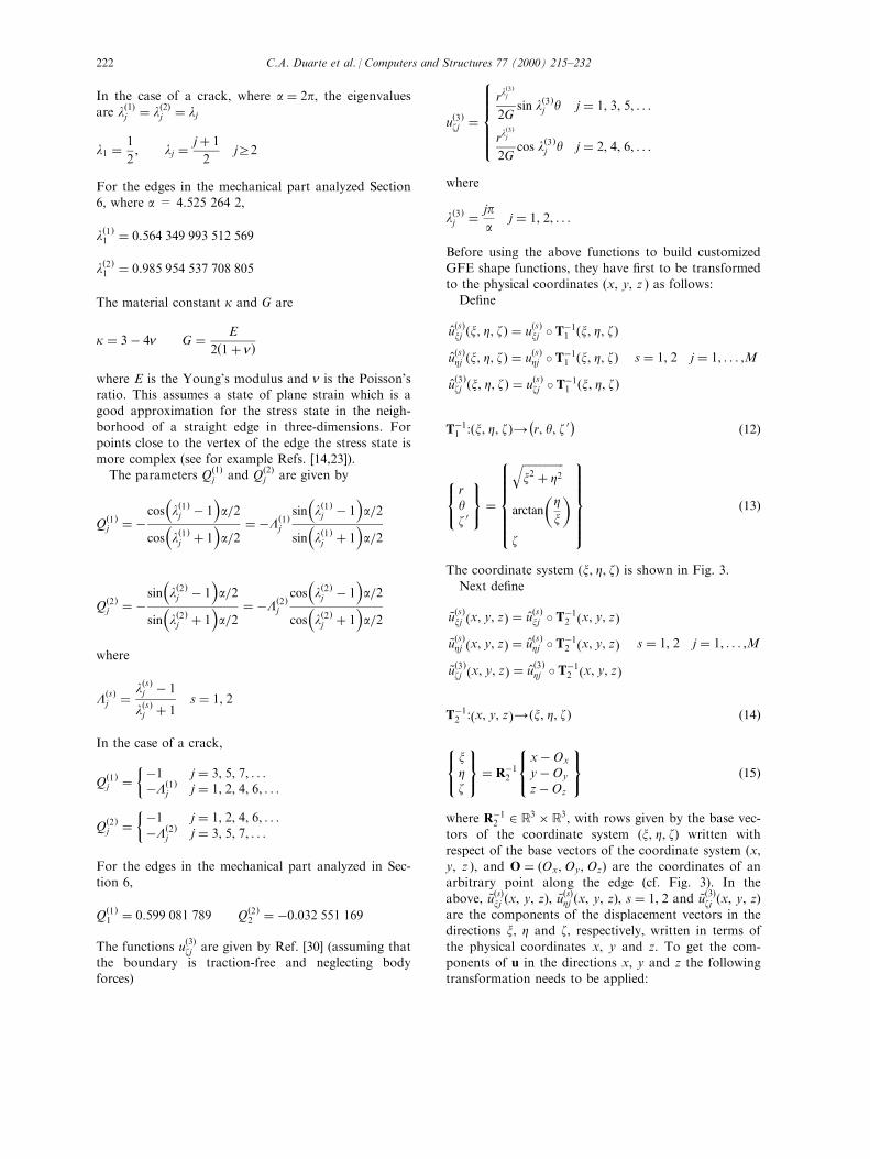
four-node quadratic generalized ®nite element, asde®ned in Eq. (2), are compared in this section.The tetrahedral mesh shown in Fig. 4 is composed

Fig. 4. Tetrahedral mesh used to investigate the structure of the sti�ness matrix in GFEMs.

Fig. 5. Non-zero entries of the sti�ness matrix for the mesh

shown in Fig. 4 with linear elements.

C.A. Duarte et al. / Computers and Structures 77 (2000) 215±232 223

of 30 elements and 24 vertex nodes. Fig. 5 shows the

structure of the sti�ness matrix for this mesh with lin-

ear tetrahedral elements. The matrix has 72 rows and

819 non-zero entries (represented by the black part of

the picture). Fig. 6(a) shows the structure of the sti�-

ness matrix when ten-node ®nite elements are used.

The matrix has 297 rows and 7,857 non-zero entries. If

generalized quadratic ®nite element approximations are

used, a sti�ness matrix is obtained with the structure

shown in Fig. 6(b). The matrix structure for the

GFEM is seen to be simpler than that of the FEM.

The GFE matrix has 288 rows and 12,672 non-zero

entries. These data are shown on Table 1. The table

also contains the number of ¯oating point operations

required for the numerical factorization of the matrices

and the computed strain energy when the model is

®xed at the left end and a uniform pressure T ��0:0, ÿ 1:0, 0:0� is applied at the right tip. The material

is assumed to be linearly elastic with Young's modulus

E = 1,000,000 PA and Poisson's ratio n � 0:3: The

following observations can be made:

1. In the case of classical ®nite elements, the non-zero

pattern of the matrix changes substantially when the

approximation is enriched from p = 1 to p = 2.

This is due to the fact that new nodes along the

edges of the tetrahedral elements must be created.

As discussed in Section 2, the p enrichment of the

approximation in the GFEM does not require the

creation of new nodes and therefore the structure of

the matrix is unchanged with p enrichment, as is

observed by comparing Figs. 5 and 6(b). It is also

observed that there are several adjacent columns in

the matrix shown in Fig. 6(b) with exactly the same

number of non-zero entries. Several modern linear

solvers can take advantage of this type of structure

to improve the performance of the factorization

Fig. 6. Non-zero entries of the sti�ness matrix for the mesh shown in Fig. 4: (a) matrix structure for ten-node quadratic tetrahedral

elements; (b) matrix structure for generalized quadratic tetrahedral elements as de®ned in Eq. (2).

Table 1

FE and GFE results for the cantilever beam shown in Fig. 4a

Method FEM/GFEM, p � 1 FEM, p � 2 GFEM, p � 2

Number of equations 72 297 288

Number of non-zeros lhs 819 7,857 12,672

Num. Float. Pt. Op. 1.595 1e+04 3.587 7e+05 7.551 4e+05

Strain energy 59.102 124 91 224.998 03 244.978 20

a The beam is ®xed at the left and a uniform pressure T � �0:0, ÿ 1:0, 0:0� is applied at the right tip.

C.A. Duarte et al. / Computers and Structures 77 (2000) 215±232224

process. One example is the Boeing sparse linear sol-

ver [28] which is used in our implementations.2. The number of equations, for the same mesh and

the same degree of approximation, is smaller in theGFEM than in the FEM (288 versus 297 equations).

This seems to be somewhat contradictory with thefact that a quadratic generalized tetrahedral elementhas 16 shape functions instead of 10 as in the classi-

cal FEM. However, in the GFEM all the dof are as-sociated with vertex nodes which are shared by

several elements (especially in a tetrahedral mesh)and therefore the assembled system of equations

will in general be smaller than in the classical FEMwhere some nodes are shared by less elements. The

ratio between the number of elements and the num-ber of nodes for the mesh shown in Fig. 4 is 30/24

= 1.25 which is quite low. In more realistic meshes,this ratio can be much larger, and consequently, the

di�erence between the dimensions of the sti�nessmatrix in the FEM and GFEM is much more pro-

nounced. One illustrative example is given in thenext section.

3. The number of non-zeros in the sti�ness matrix forthe GFEM is substantially larger than in the corre-sponding matrix for the FEM (12,672 versus 7,857).

This is a consequence of the fact that the support ofthe higher order shape functions in the GFEM is

larger than the one in the classical FEM. The sup-port of a shape functions (in the FEM or GFEM) is

equal to the union of all elements sharing the node

associated with the shape function. In the GFEM,we have only vertex nodes which are, in general,

shared by more elements than edge, face and bubblenodes used in high order ®nite elements. In the nextsection, we demonstrate that the structure of the

GFEM matrices, combined with the fact that forthe same mesh and order of approximation theirdimensions are smaller in the GFEM than in the

FEM, more than compensate for their having morenon-zeros before factorization. Our numerical exper-iments show that the factorization time is, for the

class of problems and meshes analyzed, much smal-ler for the GFEM.

6. Analysis of a structural component using GFE

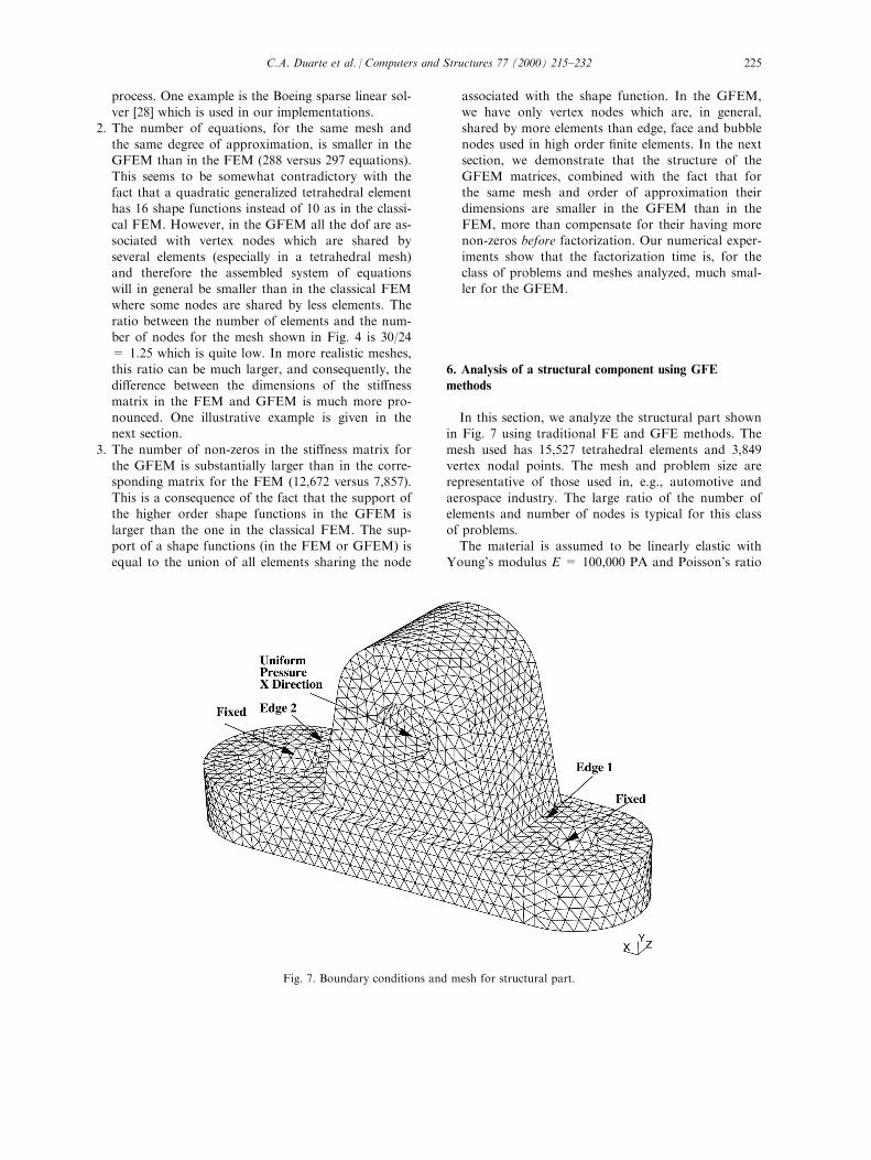
methods

In this section, we analyze the structural part shownin Fig. 7 using traditional FE and GFE methods. The

mesh used has 15,527 tetrahedral elements and 3,849vertex nodal points. The mesh and problem size arerepresentative of those used in, e.g., automotive and

aerospace industry. The large ratio of the number ofelements and number of nodes is typical for this classof problems.

The material is assumed to be linearly elastic withYoung's modulus E = 100,000 PA and Poisson's ratio

Fig. 7. Boundary conditions and mesh for structural part.

C.A. Duarte et al. / Computers and Structures 77 (2000) 215±232 225

n � 0:33: The boundary conditions are those rep-

resented in Fig. 7. The component is ®xed at both sup-ports and there is a uniformly distributed load p = 1.0in the negative x-direction applied at its upper part

(see Fig. 7). The aspect ratio of the elements in themesh are quite good. However, as we demonstratebelow, if classical FEMs are used, this mesh can not

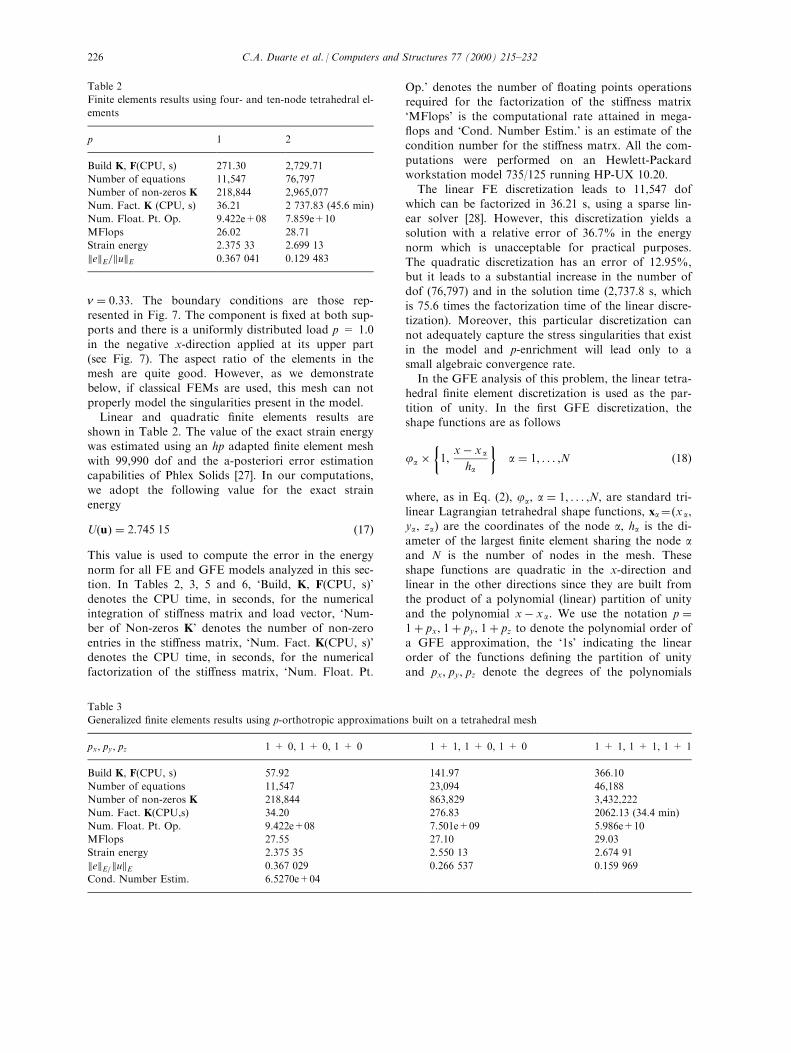
properly model the singularities present in the model.Linear and quadratic ®nite elements results are

shown in Table 2. The value of the exact strain energywas estimated using an hp adapted ®nite element mesh

with 99,990 dof and the a-posteriori error estimationcapabilities of Phlex Solids [27]. In our computations,we adopt the following value for the exact strain

energy

U�u� � 2:745 15 �17�This value is used to compute the error in the energynorm for all FE and GFE models analyzed in this sec-tion. In Tables 2, 3, 5 and 6, `Build, K, F(CPU, s)'

denotes the CPU time, in seconds, for the numericalintegration of sti�ness matrix and load vector, `Num-ber of Non-zeros K' denotes the number of non-zero

entries in the sti�ness matrix, `Num. Fact. K(CPU, s)'denotes the CPU time, in seconds, for the numericalfactorization of the sti�ness matrix, `Num. Float. Pt.

Op.' denotes the number of ¯oating points operationsrequired for the factorization of the sti�ness matrix

`MFlops' is the computational rate attained in mega-¯ops and `Cond. Number Estim.' is an estimate of thecondition number for the sti�ness matrx. All the com-

putations were performed on an Hewlett-Packardworkstation model 735/125 running HP-UX 10.20.The linear FE discretization leads to 11,547 dof

which can be factorized in 36.21 s, using a sparse lin-ear solver [28]. However, this discretization yields asolution with a relative error of 36.7% in the energy

norm which is unacceptable for practical purposes.The quadratic discretization has an error of 12.95%,but it leads to a substantial increase in the number ofdof (76,797) and in the solution time (2,737.8 s, which

is 75.6 times the factorization time of the linear discre-tization). Moreover, this particular discretization cannot adequately capture the stress singularities that exist

in the model and p-enrichment will lead only to asmall algebraic convergence rate.In the GFE analysis of this problem, the linear tetra-

hedral ®nite element discretization is used as the par-tition of unity. In the ®rst GFE discretization, theshape functions are as follows

ja ��1,

xÿ x a

ha

�a � 1, . . . ,N �18�

where, as in Eq. (2), ja, a � 1, . . . ,N, are standard tri-linear Lagrangian tetrahedral shape functions, xa��x a,ya, za� are the coordinates of the node a, ha is the di-

ameter of the largest ®nite element sharing the node aand N is the number of nodes in the mesh. Theseshape functions are quadratic in the x-direction andlinear in the other directions since they are built from

the product of a polynomial (linear) partition of unityand the polynomial xÿ x a: We use the notation p �1� px, 1� py, 1� pz to denote the polynomial order of

a GFE approximation, the `1s' indicating the linearorder of the functions de®ning the partition of unityand px, py, pz denote the degrees of the polynomials

Table 2

Finite elements results using four- and ten-node tetrahedral el-

ements

p 1 2

Build K, F(CPU, s) 271.30 2,729.71

Number of equations 11,547 76,797

Number of non-zeros K 218,844 2,965,077

Num. Fact. K (CPU, s) 36.21 2 737.83 (45.6 min)

Num. Float. Pt. Op. 9.422e+08 7.859e+10

MFlops 26.02 28.71

Strain energy 2.375 33 2.699 13

kekE=kukE 0.367 041 0.129 483

Table 3

Generalized ®nite elements results using p-orthotropic approximations built on a tetrahedral mesh

px, py, pz 1 + 0, 1 + 0, 1 + 0 1 + 1, 1 + 0, 1 + 0 1 + 1, 1 + 1, 1 + 1

Build K, F(CPU, s) 57.92 141.97 366.10

Number of equations 11,547 23,094 46,188

Number of non-zeros K 218,844 863,829 3,432,222

Num. Fact. K(CPU,s) 34.20 276.83 2062.13 (34.4 min)

Num. Float. Pt. Op. 9.422e+08 7.501e+09 5.986e+10

MFlops 27.55 27.10 29.03

Strain energy 2.375 35 2.550 13 2.674 91

kekE=kukE 0.367 029 0.266 537 0.159 969

Cond. Number Estim. 6.5270e+04

C.A. Duarte et al. / Computers and Structures 77 (2000) 215±232226

used in the construction of the GFE shape functions inthe x, y, z directions, respectively. Therefore, if only

the partition of unity is used as a basis, we have p = 1+ 0, 1 + 0, 1 + 0. For the shape functions de®ned inEq. (18) we have p = 1 + 1, 1 + 0, 1 + 0. This dis-

cretization is used to illustrate that in the GFE it ispossible to build p-orthotropic approximations regard-less of the underlying ®nite element mesh used. This

choice is also motivated by the fact that the geometry,material properties, and boundary conditions of theproblem do not change substantially in the z-direction.

In the second GFE discretization, the shape func-tions de®ned in Eq. (2) are used. In our notation, thisdiscretization is of degree p = 1 + 1, 1 + 1, 1 + 1,i.e., it is a quadratic approximation in all directions

(see Theorem 1). The GFE discretizations have dofonly at the vertices of the tetrahedral elements (fourdof for each component of the solution in the case of

the quadratic discretization). That is, there are no dofalong the edges or in the interior of the element. The p= 1 + 1, 1 + 0, 1 + 0 discretization has 23,094 dof

(exactly twice the linear discretization) and a relativeerror in the energy norm of 26.6%. The quadraticGFE discretization has 46,188 dof which is only 60%

of the number of dof in the ®nite element discretiza-tion. The total CPU time for the factorization of theresulting system of equations is 2,062.1 s, which isabout 25% smaller than in the case of quadratic ®nite

elements. The relative error in the energy norm for thisdiscretization is 16.0% which is about 23.5% largerthan in the case of quadratic ®nite elements.

The GFE results are summarized in Table 3. Thequadratic GFEM discretization leads to a smaller sys-tem of equations than comparable FEM. However, the

GFEM matrix has about 16% more non-zero entriesthan the FEM counterpart before factorization. None-theless, being a smaller matrix with a more favorablesparse structure, the GFEM matrix can be factorized

using about 24% less ¯oating point operations.

6.1. Modeling of singularities using special functions

Polynomial approximations, as used in the FE and

GFE discretizations described above, can not e�cientlyapproximate the solution in the neighborhood of geo-metric edges, such as Edges 1 and 2 shown in Fig. 7.However, asymptotic expansions of the elasticity sol-

ution in the neighborhood of such edges are wellknown and the GFE framework allows a straightfor-ward inclusion of these asymptotic ®elds in the GFE

approximation spaces, as described in Section 4. Thisapproach is demonstrated in the solution of the pro-blem represented in Fig. 7.

The same GFE discretizations described previouslyare used, but the nodes located along the Edges 1 and2 are enriched with the GFE shape functions de®ned

in Eq. (16). These functions are built from the productof the trilinear tetrahedral shape functions and the ®rst

terms of the mode I, II and III asymptotic expansionsof the elasticity solution in the neighborhood of anedge. At the vertex of those edges the elasticity sol-

ution is more complex than along the edges (see fore.g., Refs. [14,23]). This feature is ignored in the calcu-lations to be described: the same set of shape functions

are used at all nodes located along the Edges 1 and 2.The enrichment of these nodes is justi®ed by the factthat a large fraction the error is near those elements.

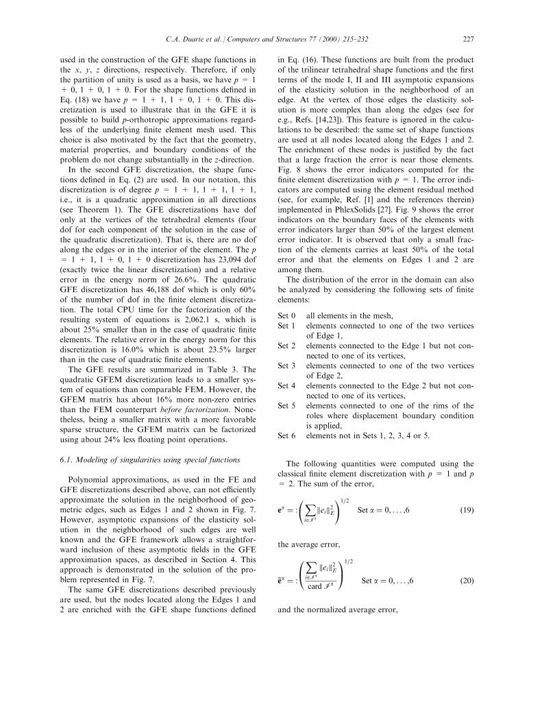
Fig. 8 shows the error indicators computed for the®nite element discretization with p = 1. The error indi-cators are computed using the element residual method(see, for example, Ref. [1] and the references therein)

implemented in PhlexSolids [27]. Fig. 9 shows the errorindicators on the boundary faces of the elements witherror indicators larger than 50% of the largest element

error indicator. It is observed that only a small frac-tion of the elements carries at least 50% of the totalerror and that the elements on Edges 1 and 2 are

among them.The distribution of the error in the domain can also

be analyzed by considering the following sets of ®nite

elements:

Set 0 all elements in the mesh,

Set 1 elements connected to one of the two verticesof Edge 1,

Set 2 elements connected to the Edge 1 but not con-

nected to one of its vertices,Set 3 elements connected to one of the two vertices

of Edge 2,

Set 4 elements connected to the Edge 2 but not con-nected to one of its vertices,

Set 5 elements connected to one of the rims of theroles where displacement boundary condition

is applied,Set 6 elements not in Sets 1, 2, 3, 4 or 5.

The following quantities were computed using theclassical ®nite element discretization with p = 1 and p= 2. The sum of the error,

ea � :

Xi2Ia

keik2E!1=2

Set a � 0, . . . ,6 �19�

the average error,

Åea � :

0@Xi2Ia

keik2Ecard Ia

1A1=2

Set a � 0, . . . ,6 �20�

and the normalized average error,

C.A. Duarte et al. / Computers and Structures 77 (2000) 215±232 227

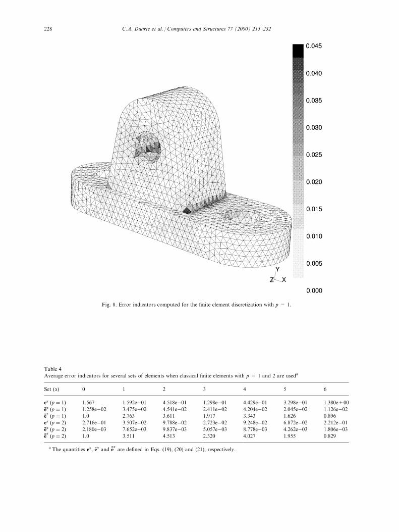
Fig. 8. Error indicators computed for the ®nite element discretization with p = 1.

Table 4

Average error indicators for several sets of elements when classical ®nite elements with p = 1 and 2 are useda

Set �a) 0 1 2 3 4 5 6

ea �p � 1� 1.567 1.592eÿ01 4.518eÿ01 1.298eÿ01 4.429eÿ01 3.298eÿ01 1.380e+00Åea �p � 1� 1.258eÿ02 3.475eÿ02 4.541eÿ02 2.411eÿ02 4.204eÿ02 2.045eÿ02 1.126eÿ02ÅÅea �p � 1� 1.0 2.763 3.611 1.917 3.343 1.626 0.896

ea �p � 2� 2.716eÿ01 3.507eÿ02 9.788eÿ02 2.723eÿ02 9.248eÿ02 6.872eÿ02 2.212eÿ01Åea �p � 2� 2.180eÿ03 7.652eÿ03 9.837eÿ03 5.057eÿ03 8.778eÿ03 4.262eÿ03 1.806eÿ03ÅÅea �p � 2� 1.0 3.511 4.513 2.320 4.027 1.955 0.829

a The quantities ea, Åea and ÅÅeaare de®ned in Eqs. (19), (20) and (21), respectively.

C.A. Duarte et al. / Computers and Structures 77 (2000) 215±232228

Fig. 9. Error indicators on the boundary faces of the elements with error indicators larger than 50% of the largest element error in-

dicator.

Table 5

Generalized ®nite elements results using p-orthotropic approximations and singular shape functions at nodes along Edges 1 and 2

px, py, pz 1 + 0, 1 + 0, 1 + 0 1 + 1, 1 + 0, 1 + 0 1 + 1, 1 + 1, 1 + 1

Build K, F(CPU,s) 201.39 428.39 936.32

Number of equations 11,943 23,490 46,584

Number of non-zeros K 244,368 904,635 3,503,592

Num. Fact. K(CPU,s) 41.22 316.23 2,156.57 (35.9min)

Num. Float. Pt. Op. 9.476e+08 7.355e+09 6.260e+10

MFlops 22.99 23.26 29.03

Strain energy 2.435 777 2.586 049 2.711 088

kekE=kukE 0.335 707 0.240 746 0.111 399

Cond. Number Estim. 7.3942e+04

C.A. Duarte et al. / Computers and Structures 77 (2000) 215±232 229

ÅÅea � :

Åea

Åea�0Set a � 0, . . . ,6 �21�

where ei is the error on the element i, Ia denotes anindex set for the Set a and k � kE denotes the energynorm. The results are shown on Table 4.

It is observed that the average error Åea for the el-ements along Edges 1 and 2 (Sets 1, 2, 3, 4) is con-siderably larger than the average error on the whole

domain (Set 0). In addition, those elements representonly a small fraction of the total number of elementsin the mesh, which justi®es our choice of using custo-

mized singular shape functions only along those edges.The results for the enriched GFE discretizations are

shown in Table 5. It is observed that the addition ofthe singular functions along the Edges 1 and 2

increases the total number of dof by only 396. This isonly 1% more dof in the case of the GFE discretiza-tion with p = 1 + 1, 1 + 1, 1 + 1 which increases

the solution time by only 4.5%. The e�ect of thisenriched shape functions on the discretization error,however, is quite noticeable. They lead to a decrease of

about 30% in the discretization error for GFE with p= 1 + 1, 1 + 1, 1 + 1. We also investigate the e�ectof additionally enriching the nodes connected to Edges

1 and 2 by a ®nite element and located at the boundaryof the part. The results for this discretization areshown in Table 6. It is observed that the e�ect of thisadditional enrichment is not substantial.

The enrichment of the GFE discretization withsingular functions leads to the issue of numerical inte-gration of these functions. In this work, our main goal

is to investigate the bene®ts of adding these functionsin terms of controling the discretization error. A su�-ciently high quadrature rule was used on the elements

with nodes carrying singular functions. The order ofthe quadrature rule was chosen so that the numericalintegration errors were small enough to not a�ect the

computed discretization errors. Table 7 shows the com-

puted strain energy and relative discretization errorkejE=kukE for the GFE discretization p = 1 + 0, 1 +0, 1 + 0 enriched with singular functions along Edges1 and 2 as a function of the number of integration

points used in the elements with nodes carrying singu-lar functions. The rules with 4, 11, 24 and 45 pointsare Keast [16] quadrature rules and the others are ten-

sor product Gaussian quadrature. The discretizationerror is computed using the reference value (17) for theexact strain energy. Based on these computations, and

the fact that we use discretizations with an error ofmore than 5%, we employ tensor product Gaussianquadrature with 1000 points on the elements with

nodes carrying singular functions. A more computa-tionally e�cient approach is, of course, to use adaptiveintegration on those elements and set the tolerance ofthe numerical integration according to the required ac-

curacy of the approximate solution.Another important issue is the e�ect of the enrich-

ment with singular functions on the condition number

of the sti�ness matrix. Estimates of the condition num-ber are shown in Tables 5 and 3. It can be observedthat the enrichment with singular functions of the

nodes along Edges 1 and 2 has no detrimental e�ecton the conditioning of the sti�ness matrix. The enrich-ment with singular functions does not lead to lineardependences as in the case of polynomial enrichment.

This last case is discussed in Section 3.

7. Conclusions

The key feature of the Generalized Finite Element

Method is the use of a partition of unity to buildthe approximation spaces. This partition of unity

Table 6

Generalized ®nite elements results using singular functions at

nodes along Edges 1 and 2 and at nodes connected to these

edges by a ®nite element and located at the boundary of the

part

px, py, pz 1 + 1, 1 + 1, 1 + 1

Build K, F(CPU, s) 1,276.36

Number of equations 47,448

Number of non-zeros K 3,646,476

Num. Fact. K(CPU, s) 2,072.94 (34.5 min)

Num. Float. Pt. Op. 6.043e+10

MFlops 29.15

Strain energy 2.712 563 9

kekE=kukE 0.108 959 8

Table 7

Computed strain energy and discretization error for various

choices of quadrature. The rules with 4,11,24 and 45 points

are Keast [16] quadrature rule). (the others are tensor product

Gaussian quadrature rule. The discretization used is GFE

with p = 1 + 0, 1 + 0, 1 + 0 and singular functions at

nodes along Edges 1 and 2

Num. Int. Pts. Strain energy kekE=kukE

4 2.458 221 212 0.323 301 264

11 2.437 851 048 0.334 580 503

24 2.436 257 160 0.335 447 063

45 2.436 024 790 0.335 573 210

216 2.436 094 921 0.335 535 142

343 2.435 938 998 0.335 619 772

512 2.435 846 523 0.335 669 954

729 2.435 777 180 0.335 707 578

1000 2.435 739 019 0.335 728 282

1331 2.435 710 261 0.335 743 883

1728 2.435 684 414 0.335 757 904

C.A. Duarte et al. / Computers and Structures 77 (2000) 215±232230

framework has several powerful properties such as

the ability to produce seamless hp ®nite element ap-proximations with nonuniform h and p, the abilityto develop customized approximations for speci®c

applications, the capability to build p-orthotropicapproximations on, e.g., 3D tetrahedral meshes, etc.Several of the so-called meshless methods proposed

in recent years also make use, explicitly or im-plicitly, of a partition of unity to build the approxi-

mation spaces [7,11,18,22]. The fundamentaldi�erence between these methods and the GFEM isin the choice of the partition of unity. In the

GFEM, the partition of unity is provided by con-ventional ®nite element methods. In this case, the

implementation of the method is essentially thesame as in standard ®nite element codes, the maindi�erence being the de®nition of the shape func-

tions. This choice of partition of unity avoids theproblem of numerical integration associated with theuse of moving least squares or Shepard partitions

of unity common to several meshless methods. Inaddition, the use of a ®nite element partition of

unity allows easy implementation of essential bound-ary conditions, which may not be a straightforwardproposition in other techniques using moving least

squares partition of unity.In this paper, we investigate several important

practical aspects of the generalized ®nite elementmethod in a 3D setting. The structure of the sti�-ness matrix in the GFEM is compared with the

®nite element counterpart when the same mesh andpolynomial degree of the approximation is used. Weshow that the structure of the matrix in the GFEM

does not change with p-enrichment, in contrast withthe classical FEM case. Modern linear solvers can

take advantage of the type of structure in the GFEmatrices to improve the performance of the factoriz-ation process. It is also demonstrated that for the

same mesh and degree of approximation, theGFEM leads to a smaller system of equations thanin the classical FEM. This di�erence in the number

of equations is specially pronounced in mesheswhere the ratio between the number of elements

and nodes in the mesh is high, as in the case oftetrahedral meshes of complex structures. This istranslated into faster solution times for the GFEM.

The GFEM framework allows for straightforwardconstruction of special solution spaces using a-priori

knowledge of properties of the solution of the pro-blem. In this paper, this is demonstrated for the caseof elasticity equations in three dimensions. This pro-

cedure does not require the modi®cation of the ®niteelement mesh. In general, these properties allows us toobtain the solution of 3D problems with higher accu-

racy and less computational e�ort than the classical®nite element method.

Acknowledgements

The work of J.T. Oden on this project was sup-ported by Army Research O�ce under grantDAAH04-96-1-0062.

References

[1] Ainsworth M, Oden JT. A posteriori error estimation in

®nite element analysis. Computational Mechanics

Advances Special Issue of Computer Methods in Applied

Mechanics and Engineering 1997;142:1±88.

[2] Babuska I, Caloz G, Osborn JE. Special ®nite element

methods for a class of second order elliptic problems

with rough coe�cients. SIAM J Numerical Analysis

1994;31(4):745±981.

[3] BabusÏ ka I, Melenk JM. The partition of unity ®nite el-

ement method. International Journal for Numerical

Methods in Engineering 1997;40:727±58.

[4] Bathe KJ. Finite element procedures in engineering

analysis. Englewood Cli�s, NJ: Prentice-Hall, 1982.

[5] Becker EB, Carey GF, Oden JT. Finite elements: an

introduction. Englewood Cli�s: Prentice-Hall, 1981

Volume I in Texas ®nite element series.

[6] Belytschko T, Krongauz Y, Organ D, Fleming M.

Meshless methods: An overview and recent develop-

ments. Computer Methods in Applied Mechanics and

Engineering 1996;139:3±47.

[7] Belytschko T, Lu YY, Gu L. Element-free Galerkin

methods. International Journal for Numerical Methods

in Engineering 1994;37:229±56.

[8] Duarte CAM. A review of some meshless methods to

solve partial di�erential equations. Technical Report 95-

06, TICAM, University of Texas at Austin, 1995.

[9] Duarte CAM, Oden JT. Hp clouds Ð a meshless method

to solve boundary-value problems. Technical Report 95-

05, TICAM, University of Texas at Austin, May 1995.

[10] Duarte CAM, Oden JT. An hp adaptive method using

clouds. Computer Methods in Applied Mechanics and

Engineering 1996;139:237±62.

[11] Duarte CAM, Oden JT. Hp clouds Ð an hp meshless

method. Numerical Methods for Partial Di�erential

Equations 1996;12:673±705.

[12] Duarte CA. The hp cloud method. PhD dissertation,

University of Texas at Austin, Austin, TX, USA,

December 1996.

[13] Du� I, Reid J. The multifrontal solution of inde®nite

sparse symmetric linear systems. ACM Trans Math

Softw 1983;9:302±25.

[14] Grisvard P. Singularities in boundary value problems.

New York: Springer-Verlag, 1982 Research notes in

Appl. Math.

[15] BabusÏ ka I, Strouboulis T, Copps K, Gangara SK,

Upadhyay CS. A-posteriori error estimation for ®nite el-

ement and generalized ®nite element method. Available

from http://yoyodyne.tamu.edu/research/error/gfem_fran-

ce.pdf.

[16] Keast P. Moderate-degree tetrahedral quadrature for-

C.A. Duarte et al. / Computers and Structures 77 (2000) 215±232 231

mulas. Computer Methods in Applied Mechanics and

Engineering 1986;55:339±48.

[17] Lancaster P, Salkauskas K. Surfaces generated by mov-

ing least squares methods. Mathematics of Computation

1981;37(155):141±58.

[18] Liu WK, Jun S, Zhang YF. Reproducing kernel particle

methods. International Journal for Numerical Methods

in Engineering 1995;20:1081±106.

[19] Melenk JM. Finite element methods with harmonic

shape functions for solving laplace's equation. Master's

thesis, University of Maryland, 1992.

[20] Melenk JM. On generalized ®nite element methods.

Ph.D. thesis, University of Maryland, 1995.

[21] Melenk JM, BabusÏ ka I. The partition of unity ®nite el-

ement method: basic theory and applications. Computer

Methods in Applied Mechanics and Engineering

1996;139:289±314.

[22] Nayroles B, Touzot G, Villon P. Generalizing the ®nite

element method: di�use approximation and di�use el-

ements. Computational Mechanics 1992;10:307±18.

[23] Nazarov SA, Plamenevsky BA. Elliptic problems in

domains with piecewise smooth boundaries. Berlin:

Walter de Gruyter, 1994 volume 13 of De Gruyter

Expositions in Mathematics.

[24] Oden JT, Duarte CA. Clouds, cracks and fem's. In:

Reddy BD, editor. Recent developments in compu-

tational and applied mechanics. Barcelona, Spain:

International Center for Numerical Methods in

Engineering, CIMNE, 1997. p. 302±21.

[25] Oden JT, Duarte CA, Zienkiewicz OC. A new cloud-

based hp ®nite element method. Computer Methods in

Applied Mechanics and Engineering 1998;153:117±26.

[26] Oden JT, Duarte CAM. Solution of singular problems

using hp clouds. In: Whiteman JR, editor. The math-

ematics of ®nite elements and applications 96. New

York, NY: Wiley, 1982. p. 35±54.

[27] PHLEXSolids. Computational Mechanics Company,

www.comco.com.

[28] The Boeing extended mathematical subprogram library.

Boeing Computer Services, Seattle, WA, USA.

[29] Strouboulis T, BabusÏ ka I, Copps K. The design and

analysis of the generalized ®nite element method.

Computer Methods in Applied Mechanics and

Engineering 2000;81(1±3):43±69.

[30] Szabo BA, Babuska I. Computation of the amplitude of

stress singular terms for cracks and reentrant corners. In:

Cruse TA, editor. Fracture Mechanics: Nineteenth

Symposium, ASTM STP 969, 1988, pp. 101±124.

[31] Barna Szabo, Babuska Ivo. Finite element analysis. New

York: Wiley, 1991.

[32] Zienkiewicz OC, Taylor RL. In: 4th ed. The ®nite el-

ement mehtod, vol. I. New York: McGraw-Hill, 1981.

C.A. Duarte et al. / Computers and Structures 77 (2000) 215±232232