A bubble-stabilized ﬁnite element method for …people.duke.edu/~jdolbow/NSF/bubble_paper.pdf ·...

INTERNATIONAL JOURNAL FOR NUMERICAL METHODS IN ENGINEERINGInt. J. Numer. Meth. Engng 2006; 69:1–21 Prepared using nmeauth.cls [Version: 2002/09/18 v2.02]

A bubble-stabilized finite element method

for Dirichlet constraints on embedded interfaces

Hashem M. Mourad1, John Dolbow1,∗, Isaac Harari2

1Department of Civil and Environmental Engineering, Duke University,Durham, North Carolina 27708, USA

2Department of Solid Mechanics, Materials, and Systems, Tel Aviv University,69978 Ramat Aviv, Israel

SUMMARY

We examine a bubble-stabilized finite element method for enforcing Dirichlet constraints on embeddedinterfaces. By embedded we refer to problems of general interest wherein the geometry of theinterface is assumed independent of some underlying bulk mesh. As such, the robust imposition ofDirichlet constraints with a Lagrange multiplier field is not trivial. To focus issues, we consider asimple one-sided problem that is representative of a wide class of evolving interface problems. Thebulk field is decomposed into coarse and fine scales, giving rise to coarse-scale and fine-scale one-sided sub-problems. The fine-scale solution is approximated with bubble functions, permitting staticcondensation and giving rise to a stabilized form bearing strong analogy with a classical method.Importantly, the method is simple to implement, readily extends to multiple dimensions, obviates theneed to specify any free stabilization parameters, and gives rise to a symmetric, positive-definite systemof equations. The performance of the method is then examined through several numerical examples.The accuracy of the Lagrange multiplier is compared to results obtained using a local version of thedomain integral method. The variational multiscale approach is shown to both stabilize the Lagrangemultiplier and improve the accuracy of the post-processed fluxes. Copyright c© 2006 John Wiley &Sons, Ltd.

key words: Embedded interface; Lagrange multiplier; finite element; stabilization

1. INTRODUCTION

Recently, much attention has focused on finite element methods employing “embedded” or“immersed” interfaces, i.e. surfaces that aren’t fitted or aligned with some underlying bulkmesh. Such techniques aim to circumvent or alleviate the difficulties associated with remeshingthe bulk domain as the interface evolves. These methods find application in a wide rangeof problems of interest to the engineering and materials science communities. For example,

∗Correspondence to: John Dolbow, Department of Civil and Environmental Engineering, Duke University,Box 90287, Durham, NC 27708-0287, USA

Contract/grant sponsor: Sandia National Laboratories; contract/grant number: 184592

Received 16 December 2005

Copyright c© 2006 John Wiley & Sons, Ltd. Revised 16 December 2005

2 H. M. MOURAD, J. DOLBOW AND I. HARARI

consider the recent work on fluid-structure interaction [1], cohesive crack growth [2], and sharpphase transitions [3], just to name a few. In this paper, we present a technique that successfullyaddresses the difficult issue of robustly enforcing Dirichlet constraints on such interfaces. Itbears emphasis that our technique is also applicable to “stiff” Neumann constraints, such asthose arising from many cohesive models.

For finite element methods that explicitly fit the mesh to the surface of interest, Dirichletconstraints are often enforced through simple collocation at the nodes on the surface. In manycases, this is sufficient to guarantee convergence. For embedded interfaces, however, such asimple approach is not readily available. Most formulations resort to a mixed method, andintroduce a Lagrange multiplier to enforce the constraint. Unfortunately, the design of finite-element subspaces for the bulk and Lagrange multiplier fields that satisfy the classical inf-supcondition proposed by Babuska [4] is not a trivial undertaking. The most convenient choicefor the discrete subspaces is often one that cannot be guaranteed stable.

In light of these difficulties, Barbosa and Hughes [5] turned to least-squares stabilizationas a means of circumventing the inf-sup condition. Stenberg [6] subsequently showed thatNitsche’s method, a classical approach for enforcing Dirichlet constraints, could be derived fromthe stabilized forms proposed by Barbosa and Hughes. Nitsche’s method [7] may be viewedas a variationally consistent penalty method, and only requires the specification of a singleparameter α to ensure stability. This classical method has garnered much attention of late, forboth meshfree methods [8] and finite element methods with embedded interfaces [9]. The issuewith Nitsche’s method, particularly for evolving interface methods, concerns the practicalityof identifying or selecting the stability constant α. Fernandez-Mendez and Huerta [8] proposedsolving a local eigenvalue problem to identify the stability constant, but this is not an efficientstrategy if required at every time step. Methods that do not rely on the specification of sucha parameter are obviously desirable.

Additional emphasis has been placed on this issue by the recent work of Ji and Dolbow [10]and Moes et al. [11] with regard to the eXtended Finite Element Method (X-FEM). The X-FEM is designed to address moving boundary value problems such as crack growth and phasetransitions without remeshing. This is effected through a combination of basis enrichment anda separation of computational and physical domains. The origins of the method can be tracedback to the work of Belytschko and Black [12] on simulating crack growth with a minimal levelof remeshing. Ji and Dolbow showed that for interfacial problems with Dirichlet constraints,the most convenient choice for Lagrange multiplier fields likely violates the inf-sup conditionfor many choices of enrichment. Moes and coworkers subsequently developed a technique fortailoring a Lagrange multiplier field to the X-FEM. They cited a sensitivity to the stabilizationconstant in Nitsche’s method, and demonstrated that their method is more robust. We note,however, that the method is not straightforward to implement, and further that it remainsunclear how to readily adapt the basic construction of their multiplier approximation to three-dimensional problems. Finally, the use of the classical Galerkin formulation to the problemgives rise to a linear algebraic system that is symmetric but not positive definite—whichprecludes the use of some fast and efficient solvers, e.g. conjugate gradient.

In this work, we approach the problem by seeking a suitable enhancement to the bulkfield. To fix ideas, we consider a simple one-sided problem involving the Laplace equationfor a bulk field on a domain with an embedded interface. The bulk field is specified on theinterface through a Dirichlet condition. We decompose the bulk field into coarse and fine scalesand introduce a model for the fine-scale field with bubble functions. Such a decomposition is

Copyright c© 2006 John Wiley & Sons, Ltd. Int. J. Numer. Meth. Engng 2006; 69:1–21Prepared using nmeauth.cls

BUBBLE STABILIZED METHOD FOR CONSTRAINTS ON EMBEDDED INTERFACES 3

inspired by the variational multiscale framework developed by Hughes [13, 14], and is relatedto the class of bubble-stabilized formulations proposed by Brezzi et al. [15] for advection-diffusion. This allows the method to correct for the lack of stability in the standard Galerkinvariational formulation of the problem. Upon making particular choices for the finite elementapproximations to the bulk field and Lagrange multiplier, we show how one can recover a formthat is very similar to Nitsche’s method. A significant feature of our approach, however, is thatit yields an element-level stabilization term αe that appears naturally via the solution of thefine-scale problem.

The use of element-level bubble functions to stabilize finite element computation originatedover twenty years ago (see, e.g., [16]). Bubble-enhanced methods [17], related to stabilizedfinite element methods [15], are seen as arising from a separation of scales according to thenumerical mesh size [18]. Methods such as the residual-free bubbles method [19, 20, 21] (relatedto the bubble-enriched nearly optimal Petrov-Galerkin method [22]), may be viewed as alocalized approach to represent the fine, unresolved, scales, within the variational multiscaleframework [13, 14]. A similar result is obtained by employing an element Green’s function [13],and the link to residual-free bubbles was explored in [23]. The obvious limitation related tothe loss of essential global effects inherent in local approaches may be overcome by employingnonconforming methods [24, 25]. The relationship of variational multiscale methods based onfine-scale Green’s functions to optimal stabilized methods with global and local character isdescribed in [26].

This paper is outlined as follows. In the next Section, we define the boundary-value problemthat will be used to study the proposed method and we provide its standard variational form.In Section 3, the details of the numerical discretization, stabilization with the variationalmultiscale method, and relationship to Nitsche’s method are presented. We also review arecent domain-integral method for computing the interfacial normal flux, considered to bean important quantity of interest for many embedded interface problems. Section 4 providesseveral numerical examples that illustrate the accuracy and robustness of the proposed method.Finally, we provide a summary and comment on future work in the last section.

2. PROBLEM STATEMENT

Consider the “one-sided problem” described by an interface Γ∗ partitioning the domain Ω intothe disjoint sets Ωc and Ω∗, as shown in Figure 1.

Perhaps the simplest one-sided boundary-value problem is given by

∆u = 0 in Ω∗ (1a)

u = ud on Γ∗ (1b)

∇u · no = h on Γh (1c)

where ∆ is the standard Laplace operator, and no is the outward unit normal to Γh, as shownin Figure 1. The above is a simplification of classical one-sided Stefan problems that arise frommodels for a wide range of evolving interface phenomena. Such models normally include anevolution equation for the geometry of the interface in which the interfacial flux

j = ∇u · n on Γ∗ (2)



Ω∗

Ωc

Γ∗

Γh

n

no

Figure 1. Notation for the one-sided problem. A domain Ω partitioned into regions Ωc and Ω∗ bythe interface Γ∗. The normal to the interface, n, is defined such that it points outward from the Ω∗

subdomain, as shown.

is a quantity of interest. For example, in many one-sided solidification problems, the normalvelocity of the interface is proportional to the interfacial flux.

2.1. Standard weak formulation

We write S for the space of admissible bulk fields, and V for the corresponding space ofvariations. We choose to enforce the constraint (1b) on Γ∗ weakly, using a Lagrange multiplierλ belonging to the space L. The weak form reads: Find (u, λ) ∈ S × L such that

∫

Ω∗

∇w · ∇u dΩ −

∫

Γ∗

wλdΓ =

∫

Γh

wh dΓ (3a)

−

∫

Γ∗

µu dΓ = −

∫

Γ∗

µud dΓ (3b)

for all (w, µ) ∈ V ×L. The Euler-Lagrange equations associated with this weak form are givenby (1) and

λ = ∇u · n (4)

3. DISCRETIZATION WITH FINITE ELEMENTS

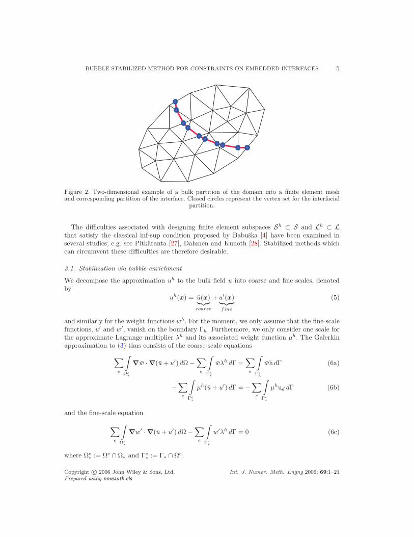
We consider a quasi-uniform partition Ωh of the domain Ω into non-overlapping elementdomains Ωe with boundaries ∂Ωe. We assume that the interface Γ∗ is approximated with apartition Γh

∗that has a particular structure; namely, the vertex set for Γh

∗is taken as the set of

intersection points between Γ∗ and the set of element edges ∂Ωe. We consider an “unfitted” or“embedded” interface method in the sense that no further assumption concerning the structureof the partition Ωh and the interface partition Γh

∗is made. For the sake of concreteness, an

example of Ωh and Γh∗

is shown in Figure 2.



Figure 2. Two-dimensional example of a bulk partition of the domain into a finite element meshand corresponding partition of the interface. Closed circles represent the vertex set for the interfacial

partition.

The difficulties associated with designing finite element subspaces Sh ⊂ S and Lh ⊂ Lthat satisfy the classical inf-sup condition proposed by Babuska [4] have been examined inseveral studies; e.g. see Pitkaranta [27], Dahmen and Kunoth [28]. Stabilized methods whichcan circumvent these difficulties are therefore desirable.

3.1. Stabilization via bubble enrichment

We decompose the approximation uh to the bulk field u into coarse and fine scales, denotedby

uh(x) = u(x)︸︷︷︸

coarse

+u′(x)︸︷︷︸

fine

(5)

and similarly for the weight functions wh. For the moment, we only assume that the fine-scalefunctions, u′ and w′, vanish on the boundary Γh. Furthermore, we only consider one scale forthe approximate Lagrange multiplier λh and its associated weight function µh. The Galerkinapproximation to (3) thus consists of the coarse-scale equations

∑

e

∫

Ωe∗

∇w · ∇(u + u′) dΩ −∑

e

∫

Γe∗

wλh dΓ =∑

e

∫

Γe

h

wh dΓ (6a)

−∑

e

∫

Γe∗

µh(u + u′) dΓ = −∑

e

∫

Γe∗

µhud dΓ (6b)

and the fine-scale equation

∑

e

∫

Ωe∗

∇w′ · ∇(u + u′) dΩ −∑

e

∫

Γe∗

w′λh dΓ = 0 (6c)

where Ωe∗

:= Ωe ∩ Ω∗ and Γe∗

:= Γ∗ ∩ Ωe.



We now consider an approximation for the coarse scale of the form

u(x) =∑

i∈I

Ni(x)ui (7a)

w(x) =∑

i∈I

Ni(x)wi (7b)

where Ni are the nodal shape functions, and I denotes the set of nodes

I = j | ωj ∩ Ω∗ 6= ∅ (8)

which have some portion of their supports ωj (with closure ωj) intersecting the domain Ω∗.For additional detail and insight into this approach, see Daux et al. [29] and other work onthe eXtended Finite Element Method. For the fine-scale approximation, we write

u′(x) =∑

e∈B

be(x)βe (9a)

w′(x) =∑

e∈B

be(x)γe (9b)

where be denotes the element-level bubble function and B is a subset of the elements in themesh given by

B = s |Ωs ∩ Γh∗6= ∅ (10)

In other words, the fine-scale solution is nonzero only in the interior of elements whose domainsintersect the interface. We remark that this restriction is only made for efficiency, and thatthe developments which follow could just as easily be applied to situations where the fine scalecontributes over all of Ω∗.

Substituting (9) into (6c) and invoking the arbitrariness of γe leads to an expression of theform

βe

∫

Ωe∗

∇be · ∇be dΩ =

∫

Γe∗

beλh dΓ −

∫

Ωe∗

∇be · ∇u dΩ (11a)

or, equivalently

βe

∫

Ωe∗

∇be · ∇be dΩ =

∫

Γe∗

be(λh − ∇u·n

)dΓ +

∫

Ωe∗

be∆u dΩ (11b)

for each e ∈ B. The above can easily be solved for the element-level fine-scale degrees offreedom βe in terms of the coarse-scale variables, yielding

βe(u, λh) =

∫

Γe∗

be(λh − ∇u·n

)dΓ +

∫

Ωe∗

be∆u dΩ

∫

Ωe∗

∇be · ∇be dΩ(12)

It is clear from this expression that the fine scales are driven by the coarse-scale residuals.



Using (9) with the coarse-scale weak form (6a, 6b) we obtain

∑

e

∫

Ωe∗

∇w · ∇u dΩ +∑

e∈B

βe

∫

Ωe∗

∇w · ∇be dΩ −∑

e

∫

Γe∗

wλh dΓ =∑

e

∫

Γe

h

wh dΓ (13a)

−∑

e

∫

Γe∗

µhu dΓ −∑

e∈B

βe

∫

Γe∗

µhbe dΓ = −∑

e

∫

Γe∗

µhud dΓ (13b)

It can be verified, after some algebraic manipulation, that substitution of (12) into (13) leads toa symmetric, positive-definite system of equations. This is a significant advantage over methodsthat simply attempt to design subspaces Sh and Lh such that the standard formulation is BB-stable.

3.2. Relation to Nitsche’s method

To show the relationship between this method and the classical one due to Nitsche [7], we nowconsider a particular choice for the approximate Lagrange multiplier λh and coarse-scale bulkfield u. Namely, we consider a piecewise-constant Lagrange multiplier, such that

λh∣∣∣Γe∗

= λe (14)

and a piecewise-linear coarse-scale field. In this case, the degrees of freedom λe can be obtainedfrom (12) and (13b) as

λe =

−∫

Γe∗

(u − ud) dΓ∫

Ωe∗

∇be · ∇be dΩ

(

∫

Γe∗

be dΓ

)2+

∫

Γe∗

be(∇u·n) dΓ −∫

Ωe∗

be∆u dΩ

∫

Γe∗

be dΓ

=

−∫

Γe∗

(u − ud) dΓ∫

Ωe∗

∇be · ∇be dΩ

(

∫

Γe∗

be dΓ

)2+ ∇u·ne (15)

where we have used the fact that a piecewise-linear field possesses a constant gradient anda vanishing Laplacian over each element domain. We have also assumed that each interfaceelement Γe

∗possesses a constant normal vector, denoted by n

e. Combining (12), (13a) and (15),rearranging terms, and performing some additional algebraic manipulations yields

∑

e

∫

Ωe∗

∇w · ∇u dΩ −∑

e∈B

∫

Γe∗

w(∇u·ne) dΓ −∑

e∈B

∫

Γe∗

u(∇w ·ne) dΓ +∑

e∈B

αe

∫

Γe∗

w dΓ

∫

Γe∗

u dΓ

=∑

e

∫

Γe

h

wh dΓ −∑

e∈B

∫

Γe∗

ud(∇w·ne) dΓ +∑

e∈B

αe

∫

Γe∗

w dΓ

∫

Γe∗

ud dΓ (16)



where the element-level penalty parameter

αe =

∫

Ωe∗

∇be · ∇be dΩ

(

∫

Γe∗

be dΓ

)2(17)

A relatively straightforward analysis shows that for an element with characteristic lineardimension h, this quantity scales like 1/h.

Nitsche’s method is a classical method for consistently penalizing Dirichlet constraints on asurface. Applied to (1), using piecewise-linear approximations, Nitsche’s method gives rise tothe Galerkin formulation∑

e

∫

Ωe∗

∇w · ∇u dΩ −∑

e∈B

∫

Γe∗

w(∇u·ne) dΓ −∑

e∈B

∫

Γe∗

u(∇w·ne) dΓ +∑

e∈B

α

∫

Γe∗

wudΓ

=∑

e

∫

Γe

h

wh dΓ −∑

e∈B

∫

Γe∗

ud(∇w·ne) dΓ +∑

e∈B

α

∫

Γe∗

wud dΓ (18)

where α is a constant parameter. Comparing with (16), the only qualitative differences concernthe element penalty parameter αe instead of a constant global parameter α, and the product ofinterface integrals versus the integral of a product on the interface. Further, Nitsche [7] showedthat α must scale like 1/h to guarantee convergence, which appears to be satisfied by (17).

Remarks

1. The element-level parameter αe follows automatically upon the choice of basis for thefine-scale solution. This is consistent with the application of the variational multiscalemethod to other classes of boundary-value problems, (e.g. see Masud and Khurram [30]and the references therein).

2. The bubble functions be in (9) are typically chosen to vanish on element boundaries ∂Ωe.Under these conditions, the fine-scale solution does not contribute to the approximationon the interface in the degenerate case when the interface aligns with an element edge.The consequences of this degenerate case are examined in Section 4, but it bears emphasisthat nothing in the above derivation specifically requires the use of such bubbles.

3. Numerical quadrature rules must be adjusted for bulk elements that are intersected bythe interface such that Ωe is partitioned between Ω∗ and Ωc, to accurately calculate thecontribution of such elements to the matrix system of equations. For details, see Dauxet al. [29].

3.3. Choice of bulk and interfacial approximations

We now discuss the specific choices we will consider for the approximations to the coarse andfine scales and the Lagrange multiplier. For simplicity, piecewise-linear Lagrange interpolantsare examined for the bulk shape functions Ni in (7). We consider both linear triangularelements and bilinear quadrilaterals.

Polynomial element bubbles are adopted for the fine-scale approximation (9). Specifically,for linear triangular elements, the function

be = ζ1 ζ2 ζ3 (19)



is used, where ζi are the classical triangular (area) coordinates. The bubble function used withbilinear quadrilateral elements is given by

be = (1 − ξ2)(1 − η2) (20)

in terms of the natural coordinates ξ and η. It is recognized that these are not necessarilythe optimal choices, and that using the optimal bubbles, or good approximations thereof, cangreatly improve the effectiveness of the overall stabilization strategy (e.g. see the work of Brezziand coworkers [17, 31] in the context of advection-diffusion problems).

We consider both piecewise-constant and piecewise-linear (i.e. λh ∈ C0(Γh∗)) approximations

to the Lagrange multiplier on Γh∗. Practically speaking, discontinuous multipliers are of the

greatest interest due to the difficulty of constructing continuous approximations for embeddedinterfaces in multiple dimensions.

3.4. Domain-integral approximation to the interface flux

In Ji and Dolbow [10], the superconvergent flux projection operator advocated by Carey andcoworkers [32, 33] was generalized to embedded interface problems. In essence, this post-processing technique employs the divergence theorem to recast surface-based evaluations intovolume (or domain) based evaluations that are better suited for weighted-residual methods.

For each node i whose support ωi intersects the interface, we first compute

ji =1

∫

Γe∗

Ni dΓ

∑

e

∫

Ωe∗∈ωi

∇Ni ·∇uh dΩ (21)

as a projection of the flux over the support of node i, with uh given by (5). The flux at anypoint on the interface is then approximated by

jh(x) =∑

i

Ni(x) ji (22)

In the next section, we will compare the accuracy of this approximation to that of the Lagrangemultiplier field on the interface.

4. NUMERICAL STUDIES

Here, we apply the ideas presented above to the following model problem

∆u = 0 in (0, 1) × (y∗, 1) (23a)

u = sin(πx) v(y∗) at y = y∗ (23b)

u = 0 at y = 1 (23c)

∇u · no = −π v(y) at x = 0, 1; y∗ < y < 1 (23d)

with known analytical solution (see [8, 34]) given by

u(x, y) = sin(πx) v(y) (24)

where v(•) := cosh(π•) − coth(π) sinh(π•). In this two-dimensional problem, the embeddedinterface Γ∗ is a horizontal line located at y = y∗, with 0 6 y∗ < 1; see Figure 3. We note that



the Dirichlet boundary condition (23c) is enforced by collocation at the nodes lying on they = 1 boundary, i.e. the space Sh of admissible bulk fields must be chosen such that all uh ∈ Sh

satisfy (23c); no Lagrange multipliers are introduced to enforce this boundary condition.

Ω∗

Ωc

Γ∗

n

no

y∗

1.0

1.0x

y

Figure 3. Geometry of the computational domain in the straight-interface model problem.

To evaluate the accuracy in the bulk field, we use the standard L2 error norm and reportnormalized, or relative norms. To evaluate the accuracy of the Lagrange multiplier on theinterface, we use the normalized error norm

Ed(λh) :=

∫

Γ∗

(λh − ∇u·n)2 dΓ

∫

Γ∗

(∇u·n)2 dΓ

1/2

(25)

Where applicable, we also report the error Ed(jh) in the normal flux, jh, obtained using the

domain-integral smoothing technique described in Section 3.4.

4.1. Results obtained on structured grids

The first series of tests is performed using structured grids of linear triangular elements. Atypical structured bulk mesh consisting of 32 triangular elements (mesh parameter h = 1/4),and the corresponding interfacial mesh are shown in Figure 4. In this case, the interface islocated at y∗ = 1/3. It is noted that the bottom row of nodes (and elements) do not contributeto the approximation uh; see Equations (7–10). The second row of nodes from the bottom,however, do contribute to the approximation since their support is partially within Ω∗. Thefinite-element solution uh obtained on a more refined mesh (h = 1/14) is shown in Figure 5.

To examine the convergence properties of the proposed method, the calculations are carriedout on a sequence of four uniform triangular meshes, with decreasing mesh parameter, h. Forconcreteness, the first two meshes are shown in Figure 6. As can be seen from this figure, thebulk partitions chosen cause the interface to always divide an underlying triangular elementinto two parts of equal height. We consider the case with the interface located at y = y∗ = 1/4.



Figure 4. Structured mesh consisting of 32 three-node triangular elements and interfacial mesh withthe interface Γ∗ located at y = y∗ = 1/3.

0

0.2

0.4

0.6

0.8

1

0.4

0.6

0.8

1

0

0.2

0.4

0.34

0.32

0.3

0.28

0.26

0.24

0.22

0.2

0.18

0.16

0.14

0.12

0.1

0.08

0.06

0.04

0.02

0

x

x

y

y

z

uh

Figure 5. Contour plot of finite-element solution uh = u + u′ for the case with y∗ = 1/3.



Figure 6. First two structured bulk and interfacial meshes in convergence study.

The errors in the bulk variable and interfacial flux are calculated and plotted against h foreach mesh. The results of this convergence study are shown in Figure 7. For the purposeof comparison, convergence results obtained with the standard mixed form (3), i.e. withoutstabilization, are presented in Figure 8.

With the bubble-stabilized method, we report linear convergence in the Lagrange multiplierand quadratic convergence in the L2-norm of the bulk field. The rate of convergence in thedomain-integral approximation to the interfacial flux is O(h1.5). With the standard mixedmethod, the error in the Lagrange multiplier increases with mesh refinement, and we notea marked decrease in the accuracy and rate of convergence in the other quantities. Whilesomewhat surprising, piecewise-constant multipliers do appear to give rise to overconstraintfor this simple embedded interface problem. This result is consistent with the observations ofMoes et al. [11].

Plots of the Lagrange multiplier, λh, and the domain-integral approximation to theinterfacial flux, jh, are shown in Figure 9 along with the analytical solution ∇u · n. Forcomparison, λh and jh, obtained without stabilization, are plotted in Figure 10. Clearly, inthis case, large spurious oscillations pollute the Lagrange multiplier solution. This pathology,which is exacerbated by mesh refinement (see Figure 8), is evidently mitigated by the proposedstabilization scheme. It is also clear from the results that the domain-integral approacheffectively smoothes the normal gradient of the bulk field on the interface, providing a muchmore accurate approximation to the interfacial flux than the piecewise-constant Lagrangemultiplier.

We also study the sensitivity of λh and jh to the location of the interface relative to theunderlying mesh. For this purpose, the distance d between Γ∗ and the closest (horizontal) rowof nodes is decreased by a factor of 2, starting from d = h/2 (the case depicted in Figure 6),down to d = h/32. The degenerate case, where the interface coincides with the underlyingelement edges (d = 0), is also considered.

The results of this sensitivity study are presented in Figure 11. For concreteness, d and h areshown for a typical pair of adjacent elements in the inset of Figure 11(a). From these results, it



Figure 7. Convergence study results for variational multiscale method on structured triangular grids.

Figure 8. Convergence study results for standard mixed method (without stabilization) on structuredtriangular grids.



-0.6

-0.4

-0.2

0

0.2

0.4

0.6

0.8

1

1.2

1.4

1.6

1.8

2

2.2

0 0.2 0.4 0.6 0.8 1

Norm

al F

lux

x

Lagrange Multiplier

Domain Integral

Analytical

Figure 9. Lagrange multiplier, domain integral, and exact flux on the interface. Results were obtainedusing a structured triangular mesh.

-40

-20

0

20

40

60

0 0.2 0.4 0.6 0.8 1

Norm

al F

lux

x

Lagrange Multiplier

Domain Integral

Analytical

Figure 10. Lagrange multiplier, domain integral, and exact flux on the interface. Results were obtainedwithout stabilization, using a structured triangular mesh.



-0.4

-0.2

0

0.2

0.4

0.6

0.8

1

1.2

1.4

1.6

1.8

2

2.2

0 0.2 0.4 0.6 0.8 1

No

rma

l F

lux

x

Lagrange Multiplier

Domain Integral

Analytical

dh

(a) d = h/2

-0.4

-0.2

0

0.2

0.4

0.6

0.8

1

1.2

1.4

1.6

1.8

2

2.2

0 0.2 0.4 0.6 0.8 1

No

rma

l F

lux

x

Lagrange Multiplier

Domain Integral

Analytical

(b) d = h/4

-3

-2

-1

0

1

2

3

4

0 0.2 0.4 0.6 0.8 1

No

rma

l F

lux

x

Lagrange Multiplier

Domain Integral

Analytical

(c) d = h/8

-0.2

0

0.2

0.4

0.6

0.8

1

1.2

1.4

1.6

1.8

2

2.2

0 0.2 0.4 0.6 0.8 1

No

rma

l F

lux

x

Lagrange Multiplier

Domain Integral

Analytical

(d) d = h/16

-0.2

0

0.2

0.4

0.6

0.8

1

1.2

1.4

1.6

1.8

2

2.2

0 0.2 0.4 0.6 0.8 1

No

rma

l F

lux

x

Lagrange Multiplier

Domain Integral

Analytical

(e) d = h/32

-0.2

0

0.2

0.4

0.6

0.8

1

1.2

1.4

1.6

1.8

2

2.2

0 0.2 0.4 0.6 0.8 1

No

rma

l F

lux

x

Lagrange Multiplier

Domain Integral

Analytical

(f) d = 0

Figure 11. Sensitivity of the Lagrange multiplier and domain-integral flux approximation to thelocation of the interface relative to the mesh. The distance d, between the interface Γ∗ and theclosest node, varies from (a) d = h/2 (see Figure 6) down to (f) d = 0 (the degenerate case). The inset

in (a) conveys the measures d and h for a typical pair of adjacent elements.



is clear that the domain-integral method yields accurate estimates of the interfacial flux, withall values of d. Conversely, the Lagrange multiplier exhibits a strong sensitivity to the locationof the interface. This can be attributed to the following. First, we note that when d = h/2,the interface is partitioned into equal segments, each having length ℓe :=

∫

Γe∗

dΓ = h/2 (see

Figure 6). As d is decreased, the ratio ℓe/h approaches zero in some segments (while, inneighboring segments, the same ratio approaches unity). This gives rise to overconstraint,manifested as oscillations in λh, which become more pronounced as d becomes smaller, e.g.see Figure 11(c). While these oscillations appear quite large, it should be emphasized that themultiplier obtained with bubble stabilization was nonetheless much more accurate than thatobtained without stabilization. Compare these to the results, for example, shown in Figure 10.

It is important to note that, with d ≪ h, be becomes negligibly small on Γe∗, and the fine-scale

solution vanishes, as implied by Equation (12). In other words, due to its reliance on elementbubbles, which vanish on element edges, the proposed stabilized method does not provide aneffective remedy for the issue discussed in the previous paragraph. The possibility of makinguse of edge bubbles to address this issue will be examined in a forthcoming paper. Here, we usea simple heuristic scheme, based on the idea that the Dirichlet constraint need not be enforcedon “short” segments, i.e. where ℓe/h is smaller than a tolerance value. Such a tolerance isoften used with embedded interface methods to determine which elements have been “cut”by the interface. The results shown in Figures 11(d) and 11(e) suggest that this strategy caneliminate overconstraint in some cases. Finally, it is observed that, in the degenerate case itself(Figure 11(f)), λh does not exhibit any large spurious oscillations.

4.2. Results obtained on unstructured grids

Consider the unstructured mesh and interface shown on the left in Figure 12. We perform aconvergence study by systematically refining this mesh by, effectively, tiling it over the domainas shown on the right of the Figure. What this approach insures, for example, is that ifthe characteristic mesh size is decreased by some factor, then so too is the dimension of theLagrange multiplier space increased. This does not necessarily occur if the sequence of meshesare constructed without care.

The convergence results for this case are shown in Figure 13. Comparing these results tothose obtained on a sequence of structured grids, we note a slight decrease in the rates ofconvergence in λh and jh to O(h0.85) and O(h0.91), respectively, as well as a slight decrease inaccuracy. The accuracy of the bulk field improves slightly however, and its convergence rateremains quadratic. We note that in each case, the tolerance discussed in the previous sectionwas not invoked. In other words, six multiplier degrees of freedom are associated with the meshshown on the left in Figure 12, one for each interfacial segment.

4.3. Curved interface

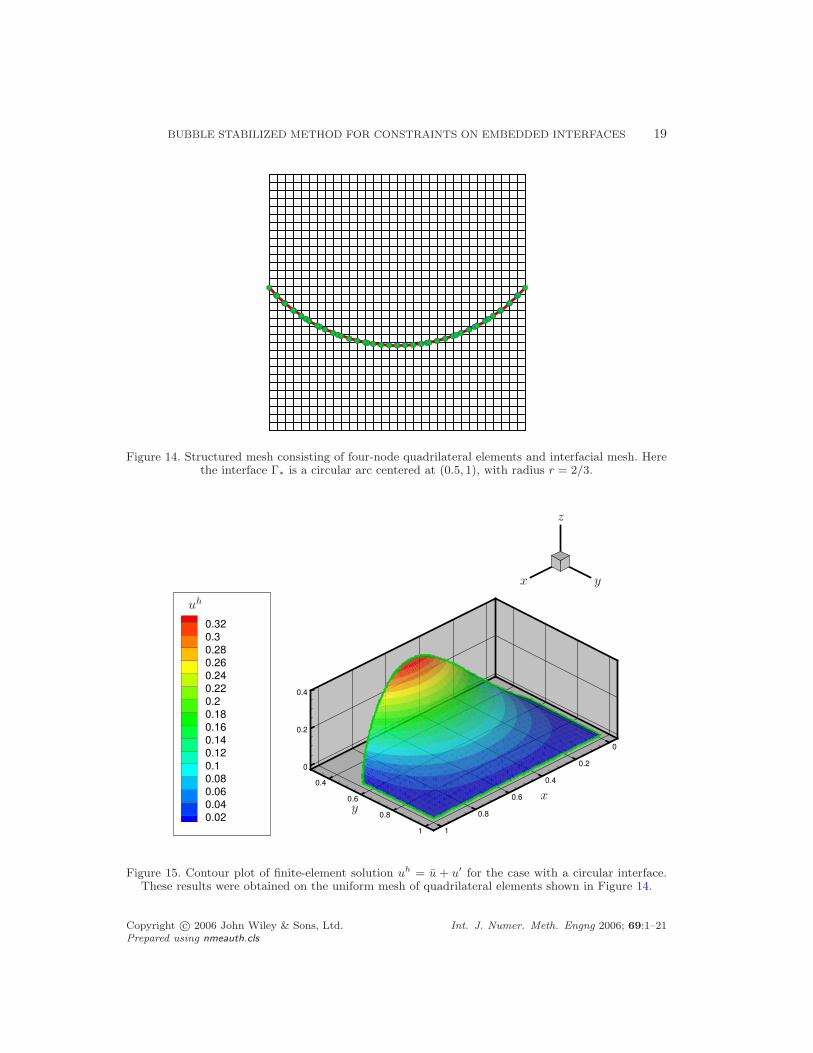
To further study the robustness of the proposed method, we consider the case of a curvedinterface. Bulk partitions consisting of bilinear quadrilateral elements are used with thismodel problem, and the accuracy and convergence characteristics are compared to thoseobtained for the same problem using linear triangular elements. We consider a modified versionof (23) as model problem, imposing a Dirichlet boundary condition that is consistent with thesolution (24) on a curved interface, in lieu of (23b). Figure 14 shows the interface geometry—a



Figure 12. First two unstructured bulk and interfacial meshes in convergence study.

Figure 13. Convergence study results for variational multiscale method on unstructured triangularmesh.



circular arc centered at (0.5, 1), with radius r = 2/3—and a typical mesh. A contour plot ofthe bulk field is shown in Figure 15.

Results pertaining to the spatial convergence of the Lagrange multipliers in this problem areshown in Figure 16. It can be seen from this figure that, in the case of quadrilateral elements,convergence is attained even with the conventional mixed method, and that stabilization doesnot affect the accuracy or rate of convergence of the results. In the case of triangular elementshowever, stabilization is clearly needed to attain convergence. It should be noted that in thisproblem, due to the mismatch between the (circular) interface geometry and the (Cartesian)mesh structure, a reduction in the bulk mesh size, h, does not necessarily cause a comparablereduction in the interfacial mesh size. Consequently, although convergence is achieved, bulkmesh refinement is not necessarily accompanied by a monotonic decrease in the error, as isevident from Figure 16. Regardless, the stabilized results were found to be well behaved forthis problem and did not exhibit any spurious oscillations in the multiplier field.

Finally, we did examine the use of piecewise-linear Lagrange multipliers for this problem inconjunction with bilinear quadrilateral elements. In this case, the rate of convergence in theLagrange multipliers remained at O(h0.3) even with the proposed stabilized method. Combinedwith the difficulties associated with constructing continuous multiplier fields for embeddedinterfaces in multiple dimensions (where Γh

∗is composed of polygonal surfaces), these findings

make it difficult to justify pursuing them in the future.

5. SUMMARY AND CONCLUDING REMARKS

In this work, we have examined the use of bubble functions to stabilize a finite element methodfor imposing Dirichlet constraints on embedded interfaces. We examined a simple modelproblem that is representative of a much wider class of formulations employing embeddedinterfaces, including those designed for cohesive crack growth and sharp phase transitions. Thechallenge is to develop a method that is stable and robust, regardless of the orientation of theinterface with respect to the underlying bulk mesh. Previous strategies have approached thisproblem by redesigning the Lagrange multiplier space or using Nitsche’s method. We showedthat with a particular choice of basis for the bulk and multiplier fields, bubble-stabilizationgives rise to a form that bears strong analogy with Nitsche. The advantage of this approachis that the stabilization parameter follows directly from the choice of bubble enrichment, andthe most convenient choice of multiplier can be used. Through several numerical examples,we showed the marked improvement in accuracy in bulk and interfacial fields that follow asa result. We also examined the accuracy of a recently developed domain-integral method. Inall cases considered, this technique was shown to provide the most accurate means to evaluatethe interfacial flux.

While our findings are promising, we have taken a relatively naive approach in selectingthe form of bubble enrichment. Our studies indicate that it may be more advantageous toconsider bubble functions that are specifically tailored to the orientation of the interface withrespect to the element/mesh. Future work along these lines will consider bubble functions thatdo not necessarily vanish along element edges. Such edge bubbles might also prove useful forstabilizing penalty methods widely used in the computational mechanics community for moreclassical, fitted finite element methods.



Figure 14. Structured mesh consisting of four-node quadrilateral elements and interfacial mesh. Herethe interface Γ∗ is a circular arc centered at (0.5, 1), with radius r = 2/3.

0

0.2

0.4

0.6

0.8

1

0.4

0.6

0.8

1

0

0.2

0.4

0.32

0.3

0.28

0.26

0.24

0.22

0.2

0.18

0.16

0.14

0.12

0.1

0.08

0.06

0.04

0.02

x

x

y

y

z

uh

Figure 15. Contour plot of finite-element solution uh = u + u′ for the case with a circular interface.These results were obtained on the uniform mesh of quadrilateral elements shown in Figure 14.



Figure 16. Convergence study results for triangular and quadrilateral grids with circular interface. Allresults shown pertain to the Lagrange multiplier field.

ACKNOWLEDGEMENTS

The support of Duke University through Sandia National Laboratories grant 184592 is gratefullyacknowledged.

REFERENCES

1. Zhang LT, Gerstenberger A, Wang X, Liu WK. Immersed finite element method. Computer Methods inApplied Mechanics and Engineering 2004; 193:2051–2067.

2. Moes N, Belytschko T. Extended finite element method for cohesive crack growth. Engineering FractureMechanics 2002; 69(7):813–833.

3. Dolbow JE, Fried E, Ji H. A numerical strategy for investigating the kinetic response of stimulus-responsivehydrogels. Computer Methods in Applied Mechanics and Engineering 2005; 194:4447–4480.

4. Babuska I. The finite element method with Lagrangian multipliers. Numerische Mathematik 1973;20(3):179–192.

5. Barbosa HJC, Hughes TJR. The finite element method with Lagrange multipliers on the boundary:Circumventing the Babuska-Brezzi condition. Computer Methods in Applied Mechanics and Engineering1991; 85(1):109–128.

6. Stenberg R. On some techniques for approximating boundary conditions in the finite element method.Journal of Computational and Applied Mathematics 1995; 63:139–148.

7. Nitsche JA. Uber ein Variationsprinzip zur Losung von Dirichlet-Problemen bei Verwendung vonTeilraumen, die keinen Randbedingungen unterworfen sind. Abhandlungen aus dem MathematischenSeminar der Universitat Hamburg 1970/71; 36:9–15.

8. Fernandez-Mendez S, Huerta A. Imposing essential boundary conditions in mesh-free methods. ComputerMethods in Applied Mechanics and Engineering 2004; 193:1257–1275.

9. Hansbo A, Hansbo P. An unfitted finite element method, based on Nitsche’s method, for elliptic interfaceproblems. Computer Methods in Applied Mechanics and Engineering 2002; 191:5537–5552.



10. Ji H, Dolbow JE. On strategies for enforcing interfacial constraints and evaluating jump conditions withthe extended finite element method. International Journal for Numerical Methods in Engineering 2004;61(14):2508–2535.

11. Moes N, Bechet E, Tourbier M. Imposing essential boundary conditions in the extended finite elementmethod. International Journal for Numerical Methods in Engineering 2006; Accepted for publication.

12. Belytschko T, Black T. Elastic crack growth in finite elements with minimal remeshing. InternationalJournal for Numerical Methods in Engineering 1999; 45(5):601–620.

13. Hughes, TJR. Multiscale phenomena: Green’s functions, the Dirichlet-to-Neumann formulation, subgridscale models, bubbles and the origins of stabilized methods. Computer Methods in Applied Mechanics andEngineering 1995; 127:387–401.

14. Hughes TJR, Feijoo GR, Mazzei L, Quincy J-B. The variational multiscale method—a paradigm forcomputational mechanics. Computer Methods in Applied Mechanics and Engineering 1998; 166:3–24.

15. Brezzi F, Bristeau MO, Franca LP, Mallet M, Roge G. A relationship between stabilized finite elementmethods and the Galerkin method with bubble functions. Computer Methods in Applied Mechanics andEngineering 1992; 96:117–129.

16. Arnold DN, Brezzi F, Fortin M. A stable finite element for the Stokes equations. Calcolo 1984; 21(4):337–344.

17. Brezzi F, Russo A. Choosing bubbles for advection-diffusion problems. Mathematical Models and Methodsin Applied Sciences 1994; 4(4):571–587.

18. Franca LP, Farhat C. Bubble functions prompt unusual stabilized finite element methods. ComputerMethods in Applied Mechanics and Engineering 1995; 123:299–308.

19. Brezzi F, Franca LP, Russo A. Further considerations on residual-free bubbles for advective-diffusiveequations. Computer Methods in Applied Mechanics and Engineering 1998; 166:25–33.

20. Franca LP, Farhat C, Macedo AP, Lesoinne M. Residual-free bubbles for the Helmholtz equation.International Journal for Numerical Methods in Engineering 1997; 40(21):4003–4009.

21. Franca LP, Nesliturk A, Stynes M. On the stability of residual-free bubbles for convection-diffusionproblems and their approximation by a two-level finite element method. Computer Methods in AppliedMechanics and Engineering 1998; 166:35–49.

22. Barbone PE, Harari I. Nearly H1-optimal finite element methods. Computer Methods in AppliedMechanics and Engineering 2001; 190:5679–5690.

23. Brezzi F, Franca LP, Hughes TJR, Russo A. b =R

g. Computer Methods in Applied Mechanics andEngineering 1997; 145:329–339.

24. Franca LP, Madureira AL, Valentin F. Towards multiscale functions: Enriching finite element spaces withlocal but not bubble-like functions. Computer Methods in Applied Mechanics and Engineering 2005;194:3006–3021.

25. Hou TY, Wu XH. A multiscale finite element method for elliptic problems in composite materials andporous media. Journal of Computational Physics 1997; 134(1):169–189.

26. Hughes TJR, Sangalli G. Variational multiscale analysis: The fine-scale Green’s function, projection,optimization, localization, and stabilized methods. Institute for Computational Engineering and Sciences(ICES) Report 05-46 ; The University of Texas: Austin, November 2005.

27. Pitkaranta J. Boundary subspaces for the finite element method with Lagrange multipliers. NumerischeMathematik 1979; 33(3):273–289.

28. Dahmen W, Kunoth A. Appending boundary conditions by Lagrange multipliers: analysis of the LBBcondition. Numerische Mathematik 2001; 88(1):9–42.

29. Daux C, Moes N, Dolbow J, Sukumar N, Belytschko T. Arbitrary branched and intersecting cracks withthe extended finite element method. International Journal for Numerical Methods in Engineering 2000;48(12):1741–1760.

30. Masud A, Khurram RA. A multiscale finite element method for the incompressible Navier-Stokes equations.Computer Methods in Applied Mechanics and Engineering; in press.

31. Brezzi F, Marini D, Russo A. Applications of the pseudo residual-free bubbles to the stabilization ofconvection-diffusion problems. Computer Methods in Applied Mechanics and Engineering 1998; 166:51–63.

32. Carey GF, Chow SS, Seager MK. Approximate boundary-flux calculations. Computer Methods in AppliedMechanics and Engineering 1985; 50(2):107–120.

33. Pehlivanov AI, Lazarov RD, Carey GF, Chow SS. Superconvergence analysis of approximate boundary-fluxcalculations. Numerische Mathematik 1992; 63(4):483–501.

34. Wagner Gj, Liu WK. Hierarchical enrichment for bridging scales and mesh-free boundary conditions.International Journal for Numerical Methods in Engineering 2001; 50(3):507–524.


A bubble-stabilized ﬁnite element method for …people.duke.edu/~jdolbow/NSF/bubble_paper.pdf ·...

Documents

Transcript of A bubble-stabilized ﬁnite element method for …people.duke.edu/~jdolbow/NSF/bubble_paper.pdf ·...