Validation of the multiscale mixed ﬁnite-element method

INTERNATIONAL JOURNAL FOR NUMERICAL METHODS IN FLUIDSInt. J. Numer. Meth. Fluids2010;00:1–17Published online in Wiley InterScience (www.interscience.wiley.com). DOI: 10.1002/fld

Validation of the multiscale mixed finite-element method

Mayur Pal1∗, Sadok Lamine2, Knut-Andreas Lie3, and Stein Krogstad3

1 Maersk Oil and Gas, Denmark2 Shell Intl., Netherlands,

3 SINTEF ICT, P.O. Box 124, Blindern, N–0314 Oslo, Norway

SUMMARY

Subsurface reservoirs generally have a complex description in terms of both geometry and geology. Thisposes a continuing challenge in modeling and simulation of petroleum reservoirs due to variations of staticand dynamic properties at different length scales. Multiscale methods constitute a promising approach thatenables efficient simulation of geological models while retaining a level of detail in heterogeneity that wouldnot be possible via conventional upscaling methods.Multiscale methods developed to solve coupled flow equations for reservoir simulation are based on ahierarchical strategy in which the pressure equation is solved on a coarsened grid and the transport equationis solved on the fine grid, and the two equations are treated asa decoupled system. In particular, themultiscale mixed finite-element (MsMFE) method attempts tocapture sub-grid geological heterogeneitydirectly into the coarse-scale equations via a set of numerically computed basis functions. These basisfunctions are able to capture the predominant multiscale information and are coupled through a globalformulation to provide good approximation of the subsurface flow solution.In the literature, the general formulation of the MsMFE method for incompressible two-phase andcompressible three-phase flow has mainly addressed problems with idealized flow physics. In this paper,we first outline a recent formulation that accounts for compressibility, gravity, and spatially-dependent rock-fluid parameters. Then, we validate the method by evaluatingits computational efficiency and accuracy ona series of representative benchmark tests that have a high degree of realism with respect to flow physics,heterogeneity in the petrophysical models, and geometry/topology of the corner-point grids. In particular,the MsMFE method is validated and compared against an industry-standard fine-scale solver. The fine-scaleflux, pressure, and saturation fields computed by the multiscale simulation show a noteworthy improvementin resolution and accuracy compared with coarse-scale models. Copyright c© 2010 John Wiley & Sons, Ltd.

Received . . .

KEY WORDS: Multiscale methods; mimetic methods; basis functions; geological modeling; reservoirsimulation; upscaling; fractures and barriers

1. INTRODUCTION

In the past few years, there has been an increasing interest in multiscale methods for a widevariety of engineering problems. The research in the area ofmultiscale methods is primarilymotivated by the complexity and inherent multiscale natureof problems across a wide range ofengineering disciplines, the rapid growth of computational power, and the need to solve highlydetailed multiscale problems accurately and efficiently. For most engineering problems that involvea wide span of scales, it is often sufficient to accurately predict the macroscale behavior of

∗Correspondence to: Maersk Oil and Gas, Esplanden 50, Copenhagen, Denmark. (This work was carried out while theauthor worked at Shell Intl.) E-mail: [email protected]

Contract/grant sponsor: Publishing Arts Research Council; contract/grant number: 98–1846389

Copyright c© 2010 John Wiley & Sons, Ltd.

Prepared usingfldauth.cls [Version: 2010/05/13 v2.00]

2 M. PAL ET AL.

the system and it is not possible, or simply too expensive, toperform simulations that providequantitative information about physical processes at all relevant scales, even with modern daycomputers. However, accounting for macroscopic effects only may not give the accuracy requiredbecause small-scale properties usually have a significant impact on the macroscale behavior. Apopular approach to resolve this problem, is to assume scaleseparation, which means that one candefine distinct characteristic scales for processes/effects that take place on the macroscopic scaleand can be resolved on a computational grid, and processes/effects that take place locally on thesubgrid scale. So-called multiscale methods [1, 2] are designed to accurately and effectively solveproblems having multiple scales and offer a systematic framework for incorporating effects from anunresolved scale into the global flow equations in a manner that is consistent with the underlyingdifferential operators. To accurately account for fine-scale effects in the macroscopic description,most multiscale methods rely on fine-scale computations that only use information within localregions to build effective parametrizations of the fine-scale behavior.

The flow of hydrocarbons in subsurface rock formations is an example of multiscale processesthat do not have apparent scale separation. In many aspects,such problems are more challengingbecause nonlocal information is needed if one wants to compute effective properties that accuratelyrepresent subgrid effects. As a result, most existing multiscale methods rely on sophisticatedcombinations of fine-scale and coarse-scale computations to resolve the most important fine-scaleinformation efficiently without having to compute directlyon the global fine-scale problem. Forpetroleum reservoir simulation, in particular, multiscale methods are formulated so that fine-scalepetrophysical and geological effects are captured directly in the coarse-scale simulation modelwithout the need for explicit computation of effective properties.

Quite a number of such multiscale methods have been presented in the literature, including dual-grid methods [3, 4, 5, 6], finite-element methods [7], mixed finite-element [8, 9, 10, 11], andfinite-volume methods [12, 13, 14, 15, 16, 17]. Apart from algorithmic differences, all of thesemethods share the same basic concept of incorporating fine-scale information into the coarse-scale equations via some sort of numerically constructed functions. These functions, also knownas basis functions [7], contain fine-scale information embedded in the solution and are coupledthrough a global formulation to provide an accurate approximation of the flow solution. In a typicalmultiscale method, the pressure is first solved on a coarse grid and then propagated to a muchfiner grid using the basis functions. These basis functions can be computed locally, globally, or byusing an adaptive-local global approach [11] to fill in the details of the fluxes that are required tosubsequently compute the saturation change on the finer grid. In this two-grid approach, the pressureand saturation equations are decoupled. The pressure equation is solved on a coarse grid and a mass-conservative fine-scale flux field is recovered to solve the transport equation on the underlying finegrid. Most of the multiscale methods presented to date aim atcapturing sub-scale pressure solutionswith a predominantly elliptic nature.

Despite their obvious similarities, multiscale methods should not be confused with upscaling.A comprehensive comparison of multiscale methods with state-of-the-art upscaling methods forelliptic problems in porous media is presented in [18]. The main objective of the multiscale methodis to efficiently obtain an accurate approximation to the fine-scale solution, whereas the intent ofupscaling is to generate approximate coarse-scale solutions [19, 20]. Moreover, the natural couplingof local and global scales in multiscale methods reduces inconsistency and non-physical coarse-scale properties that are often associated with many upscaling techniques.

To date, there are almost no papers that validate multiscalemethods on cases containing thecomplexity in geology and flow physics seen in real-life models used in industry. Herein, ourmain purpose is to present the result of such a validation study in which the multiscale mixedfinite-element method is applied to simulate two-phase, incompressible flow on challenging andgeologically realistic corner-point grids for cases including gravity and relative-permeability andcapillary functions that vary with rock type. As part of the validation, the method is benchmarkedagainst an industry-standard simulator. We also present preliminary test results for an idealized caseof compressible two-phase flow described by the black-oil equations and discuss what we perceiveas the main challenges in extending the method to more complex flow physics.

Copyright c© 2010 John Wiley & Sons, Ltd. Int. J. Numer. Meth. Fluids(2010)Prepared usingfldauth.cls DOI: 10.1002/fld

VALIDATION OF THE MSMFE METHOD 3

The multiscale formulations presented in this paper have been implemented in the open-sourceMATLAB Reservoir Simulation Toolbox (MRST) [21] which can be downloaded and freely usedunder the GNU General Public License (GPLv3). The numericalresults presented in this paper aregenerated using functionality from themsmfem module in MRST.

This paper is organized as follows: the mathematical equations governing flow in porous mediumare briefly reviewed in Section2. Section3 presents the basics of the multiscale mixed finite-elementformulation and also outlines how to extend the method to incorporate compressibility, capillary, andgravity forces. Numerical results are presented in Section4, followed by a summary and concludingremarks in Section5.

2. MATHEMATICAL MODEL AND FINE-SCALE DISCRETIZATION

The partial differential equations governing two-phase incompressible flow in a porous medium canbe derived from the continuity equation over an arbitrary domainΩ, given for phasei as follows:

φ∂Si

∂t+∇~vi = qi, (1)

and Darcy’s law describing relationship between the phase velocity~vi and phase pressurepi,

~vi = −Kλi(∇pi − gρi∇z). (2)

Here,φ and K denote porosity and permeability, which are both both represented in terms ofconstant values inside the cells of a space-filling, volumetric grid. Each phasei is described bya densityρi, a saturationSi, a fluid source/sinkqi, and a phase mobilityλi = kri/µi, whereµi

denotes the viscosity andkri the relative permeability, i.e., the reduced permeabilityobserved byone fluid phase in the presence of the other phase. Finally,g is the gravity constant andz the verticalcoordinate. To obtain a solvable system, we need to define some closure relations. Herein, we onlyconsider two phases, water (w) and oil (o), which are assumedto fill the pore volume so thatSo

+Sw ≡ 1. Moreover, the two fluid pressures are related by the capillary pressurepc = po − pw,which is assumed to be given as a function of fluid saturation.

In an incompressible model, pressure signals propagate with an infinite speed whereas fluidsare displaced by fronts that travel at a finite speed. To better represent these different physicalcharacteristics, it is common to reformulate the model equations as one equation for pressure andone equation for transport. The pressure equation is elliptic while the transport equation is generallyparabolic but has a strong hyperbolic character. To this end, we define the flow rateq = qo + qwand introduce the total mobilityλt = λw + λo, the fractional flow functionfi = λi/λt, and the totalvelocity~vt = ~vw + ~vo. Then we can derive the following equation for oil pressure and total velocity,

∇ · ~v = q, ~v = −Kλ[

∇po − g(Sw)∇z + h(Sw)∇pc]

, (3)

and an evolution equation for the water saturation

φ∂Sw

∂t+∇ · fw(Sw)

[

~v +Kλo(Sw)(

(ρw − ρo)g∇z +∇pc(Sw))]

=qwρw. (4)

Here, g(Sw) = [fw(Sw)ρw + fo(Sw)ρo]g represents gravity effects and the form of the functionh(Sw) depends upon the choice of primary pressure variable; if we choose oil pressure,h(Sw) =fw(Sw). For simplicity, we will henceforth drop the subscripts on the primary variablesp andS.

2.1. Pressure equation

To solve the system (3)–(4) numerically, the computational domainΩ is partitioned into a set ofNnon-overlapping polyhedral cells. Each cellCi can have an arbitrary number ofni planar faces, andeach face matches the face of a neighboring cell. Letui denote the vector of outward fluxes from


4 M. PAL ET AL.

cellCi, pi denote the pressure at the cell center, andπi the pressure at the cell faces. We then applya standard, locally conservative discretization of Darcy’s law

ui = T i

[

eipi − πi

]

, ei = (1, ..., 1)T , (5)

whereT i is the matrix of one-sided transmissibilities. In the presence of gravity and capillary forces,the discretization takes the form,

ui = T i

[

eipi − πi − g(Si)∆zi + h(Si)(

eipc(~xi, Si)− pci

)]

. (6)

Here,∆zi denotes the vector of differences in thez-coordinate of the cell center~xi and the facecentroids. The capillary pressurepci at the cell faces is discretized using a standard two-point flux-approximation (TPFA) method.

By augmenting (6) with flux and pressure continuity across cell faces, we can derive the followingdiscrete linear system for the global flow problem,

B C D

CT0 0

DT0 0

u

−p

π

=

−G(S)∆z +H(S)∆pc

q

0

. (7)

Here,u denotes the outward face fluxes ordered cell wise (fluxes overinterior faces and faultsappear twice with opposite signs),p denotes the cell pressure, andπ the face pressures.

To solve (7), we use a block-wise Gaussian elimination to give a positive definite system (theso-called Schur complement) for the face pressures

(

DTB−1D − F TL−1F)

π = F TL−1q, (8)

whereF = CTB−1D andL = CTB−1C. Once the face pressures have been computed, the cellpressures and fluxes can be reconstructed by back-substitution,

Lp = q + Fπ, Bu = Cp−Dπ.

The disadvantage of using the hybrid formulation (7) is that we get a linear system withsignificantly more degrees-of-freedom than for a straightforward cell-centered two-point scheme;the advantage is that the general form (7) includes consistent discretizations like multipoint andmimetic schemes, and as we shall see later, the multiscale mixed finite-element method. In termsof computational costs, we also notice that the Schur complement only involvesB−1 which canbe constructed algebraically for many numerical schemes including, in particular, the standard two-point method, mimetic methods [22, 23, 24], and the MPFA-O method [25, 26, 27]. Moreover, thematrixL is by construction diagonal and hence simple to invert.

2.2. Transport equation

The transport equation (4) is solved on the fine-scale grid using a standard discretization based onupstream-weighted mobilities. In the absence of gravity and capillary forces, the resulting schemereads

Sn+1 = Sn −∆tV −1UF (Sm)−max(q, 0)− f(Sm)min(q, 0))

. (9)

Here,V is a diagonal matrix of pore volumes, whileU is a matrix with dimension equal the numberof cells times the number of faces giving the flux contribution from Darcy fluxes for each face.Finally, F denotes the upstream-weighted fractional flow evaluated per face andf the fractionalflow function evaluated per cell. The discretization may be explicit (m = n) or implicit (m = n+ 1)and the numerical accuracy can (of course) be improved by using higher-order upwind schemes, likethe wave-oriented multi-dimensional schemes [28, 29].

Gravity effects are added by using upstream weighting in a straightforward manner. Furthermore,we use two-point differences to compute the contributions from the gradient of the capillary pressure(∇pc) on a face between two neighboring cellsi, j.

K∇pc(S) ≈ Kh

(

pc(Si)− pc(Sj))

/|~cij |, (10)

where~cij is the centroid difference between cellsi andj andKh denotes the harmonic average ofthe cell permeabilities in the direction of the face normal.



3. THE MULTISCALE MIXED FINITE-ELEMENT METHOD

The early concepts of mixed multiscale finite-element (MsMFE) methods for solving Poisson-typeelliptic equations,

∇ · ~v = f, ~v = −λ(x)∇p, in Ω, (11)

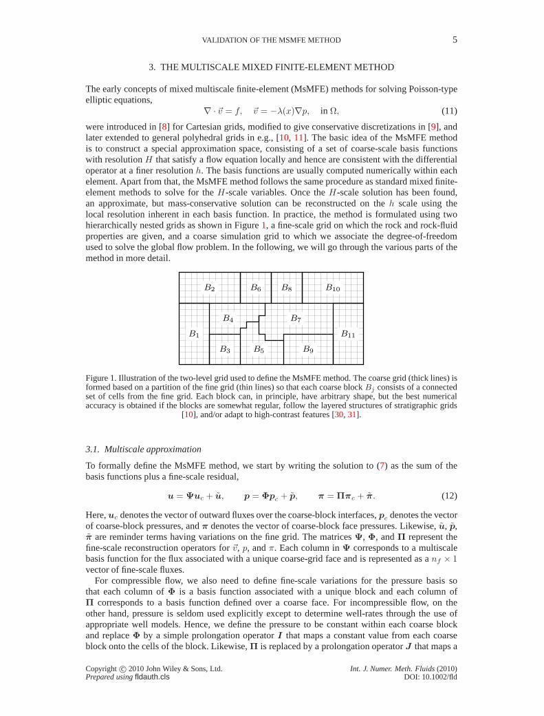
were introduced in [8] for Cartesian grids, modified to give conservative discretizations in [9], andlater extended to general polyhedral grids in e.g., [10, 11]. The basic idea of the MsMFE methodis to construct a special approximation space, consisting of a set of coarse-scale basis functionswith resolutionH that satisfy a flow equation locally and hence are consistentwith the differentialoperator at a finer resolutionh. The basis functions are usually computed numerically within eachelement. Apart from that, the MsMFE method follows the same procedure as standard mixed finite-element methods to solve for theH-scale variables. Once theH-scale solution has been found,an approximate, but mass-conservative solution can be reconstructed on theh scale using thelocal resolution inherent in each basis function. In practice, the method is formulated using twohierarchically nested grids as shown in Figure1, a fine-scale grid on which the rock and rock-fluidproperties are given, and a coarse simulation grid to which we associate the degree-of-freedomused to solve the global flow problem. In the following, we will go through the various parts of themethod in more detail.

B1

B2

B3

B4

B5

B6

B7

B8

B9

B10

B11

Figure 1. Illustration of the two-level grid used to define the MsMFE method. The coarse grid (thick lines) isformed based on a partition of the fine grid (thin lines) so that each coarse blockBj consists of a connectedset of cells from the fine grid. Each block can, in principle, have arbitrary shape, but the best numericalaccuracy is obtained if the blocks are somewhat regular, follow the layered structures of stratigraphic grids

[10], and/or adapt to high-contrast features [30, 31].

3.1. Multiscale approximation

To formally define the MsMFE method, we start by writing the solution to (7) as the sum of thebasis functions plus a fine-scale residual,

u = Ψuc + u, p = Φpc + p, π = Ππc + π. (12)

Here,uc denotes the vector of outward fluxes over the coarse-block interfaces,pc denotes the vectorof coarse-block pressures, andπ denotes the vector of coarse-block face pressures. Likewise, u, p,π are reminder terms having variations on the fine grid. The matricesΨ, Φ, andΠ represent thefine-scale reconstruction operators for~v, p, andπ. Each column inΨ corresponds to a multiscalebasis function for the flux associated with a unique coarse-grid face and is represented as anf × 1vector of fine-scale fluxes.

For compressible flow, we also need to define fine-scale variations for the pressure basis sothat each column ofΦ is a basis function associated with a unique block and each column ofΠ corresponds to a basis function defined over a coarse face. For incompressible flow, on theother hand, pressure is seldom used explicitly except to determine well-rates through the use ofappropriate well models. Hence, we define the pressure to be constant within each coarse blockand replaceΦ by a simple prolongation operatorI that maps a constant value from each coarseblock onto the cells of the block. Likewise,Π is replaced by a prolongation operatorJ that maps a


6 M. PAL ET AL.

−~ψij = −Ki∇φij

∇ · ~ψij = ωi(~x)

Bi

−~ψij = −Kj∇φij

∇ · ~ψij = −ωj(~x)

Bj

Figure 2. Illustration of the generation of a two-block basis function for the associated with the coarse fluxacross the interfaceΓij between two coarse blocksBi andBj . Here, the blocks are rectangular, but the exact

same construction applies to general polygonal/polyhedral blocks.

constant value from each coarse face onto the individual cell faces of the coarse face. Altogether, thisdefines a reconstruction operatorR = diag(Ψ, I,J) that enables us to map the degrees-of-freedomxc = [uc,−pc,πc] on the coarse-scale to the corresponding fine-scale quantitiesx = [u,−p,π].

3.2. Coarse system

To form a global system on the coarse grid, we need a compression operator that will bring thefine-scale system (7) to the space spanned by our multiscale basis functions. Here,RT is a naturalchoice since the transposed of the prolongation operatorsI andJ correspond to the sum over allfine cells of a coarse block and all fine-cell faces that are part of the faces of the coarse blocks,respectively. Multiplying (7) from the left byRT, substitutingx = Rxc, and rearranging terms, weobtain

ΨTBΨ Ψ

TCI ΨTDJ

ITCTΨ 0 0

JTDTΨ 0 0

uc

−pc

πc

=

ΨT(

H(S)∆pc −G(S)∆z)

IT q

0

. (13)

On the right-hand side, the fine-scale reminder terms were eliminated as follows:p disappears if weinterpret the coarse-scale pressure as thew-weighted average of the true pressure,pic =

∫

Bi

wp d~x,wherew is the source term used to define basis functions, see Section3.3. The two other terms,uandπ, are simply neglected. The coarse system (13) is on the same hybrid form as the fine-scalesystem (7) and can be solved using the Schur-complement reduction discussed in Section2.1.

3.3. Multiscale basis functions

The basis function associated with a flux between two coarse blocks is constructed as illustratedin Figure2. The resulting method is not convergent, but will typicallygive reasonable accuracyon finite grids. The purpose of the weight functionwij(~x) is to distribute∇ · ~v over the coarseblock. To ensure a unit flow across the interfaceΓij , the weight function should be chosen onthe formwi(x) = θ(x)/

∫

Bi

θ(x)dx. The functionθ(x) can be defined in several ways [32, 33].For incompressible flow, the simplest choice is to setθ(~x) ≡ 1 or θ(~x) = trace(K) away from thepossible wells andθ(~x) = q(~x) in grid blocks penetrated by wells. This will reproduce the lowest-order Raviart–Thomas basis on rectangular blocks with homogeneous, isotropic permeability. Forincompressible flow, the pressure is immaterial andφij can be replaced by a constant inside eachblock.

3.4. Capillary forces

To account for capillary forces, we introduce an additionalset of basis functions defined as

~ψpij = −K

(

∇φcij − h(S)∇pc(S))

, ∇ · ~ψcij = 0, (14)

so that there are two flux bases associated with each coarse face. The new basis functions areincluded in the multiscale expansion (12) and in the coarse-scale system (13) by adding each



discrete approximation to~ψpij as an extra column inΨ. In other words,Ψ0 denotes the basis

functions defined in Section3.3andu0c the corresponding degrees of freedom, thenuc = [uc0 up

c ]anduc = [uc0 up

c ].Using an extra set of basis functions instead of adding capillary effects directly in the basis

functions ~ψij has the advantage that we avoid the problem of having to scalethe relativecontributions of the physical capillary terms and the artificial source termwij . I also reduces thesaturation dependence in our set of basis functions.

3.5. Compressibility

The basic flow model (3) can be extended to compressible flow as follows

∇ · ~v = q − ct∂p

∂t+(

γ(S, p)~v + β(p)Kg∇z)

· ∇p, ~v = −λK(

∇p− g(S)∇z)

, (15)

wherect denotes total compressibilities andβ(p) andγ(S, p) are known functions of pressure- andsaturation-dependent parameters. For simplicity, we neglect capillary forces and write the linearizeddiscrete system on mixed form

[

Bn C

CT P n(pn+1

ν+1)

] [

vn+1

ν+1

−pn+1

ν+1

]

=

[

fn(pn+1ν )

gn(pn,pn+1ν )

]

. (16)

Here,ν indicates iterations in a nonlinear solver and superscriptn indicates functional dependenceon saturation/pressure from the previous time step; this superscript will be dropped for brevity.

MsMFE methods for systems on the form (16) have been discussed in detail in [34, 33]. Forcompressible flow, the pressure is no longer immaterial andφij should thus include subscalepressure variations. To ensure that pressure and flux bases scale similarly, we use a saturation-dependent decomposition for pressure,p = Ipc +ΛΦvc + p, whereΛ = diag(λ0ℓ/λℓ) andλ0ℓ isthe mobility used to calculate basis functionℓ. This gives the coarse-scale system

[

ΨTBΨ Ψ

TCI

IT (CTΨ− P νΛΦ) ITP νI

]

[

vν+1c

−pν+1c

]

=

[

ΨTfν

IT gν

]

, (17)

which needs to be solved iteratively to construct a multiscale approximation. To get a fine-scaleapproximation that converges to zero fine-scale residual, we need to include an equation for theresidual terms that were neglected in (17)

[

B C

CT P

] [

vν+1

−pν+1

]

=

[

f c −ΨTBΨvc +Ψ

TCIpc

gc − IT (CTΨ− P νΛΦ)vc + ITP νIpc

]

. (18)

If the residuals have a localized structure, this equation can be solved efficiently by a standardoverlapping Schwarz method. Hence, the resulting iterative method, iMsMFE for short, consists ofan outer loop, in which we iterate over (17) and (18) to reduce the fine-scale residual, and two innerloops that are used to solve (17) and (18), respectively.

4. NUMERICAL RESULTS

In this section, we will validate the MsMFE method on five different test cases with realisticreservoir geometries and petrophysical properties, as well as on models with spatially dependentfluid properties. The aim of the first test case is to assess thecomputational efficiency of the methodon a large-scale geological model with approximately 700,000 cells. The second test case comparesthe performance of the multiscale method with the Shell standard simulator [35]. Case three andfour aim to validate the multiscale method for incompressible two-phase flow with gravity andspatially-dependent rock-fluid parameters. Case three involves two regions with different relative


8 M. PAL ET AL.

permeability and capillary curves, whereas the fourth casecorresponds to a sector model withmultiple rock types, with a different relative permeability and capillary curve associated with eachrock type. The final test case demonstrates the use of MsMFE for compressible two-phase flowdescribed by the black-oil equations.

To perform the numerical experiments, the MsMFE methods described above have beenimplemented as software prototypes in Matlab, using the Matlab Reservoir Simulation Toolbox(MRST) [36]; all examples except for the fifth were computed with functions that are publiclyavailable in themsmfem module in MRST Release 2011b [21] and later. The main purposeof MRST is to simplify the prototyping and testing of new computational methods on generalunstructured grids. This means that computational efficiency has been sacrificed in certain casesfor the sake of generality and flexibility of the toolbox. In particular, the data structure used torepresent basis functions in themsmfem module introduces significant computational overheadwhen extracting basis functions to assemble coarse systems. To get a more reliable assessment ofthe computational efficiency of the MsMFE method, we have developed a C-accelerated version ofthe incompressible method, in which all steps except for thelinear solver of the coarse system areperformed in C via a MEX interface to Matlab. Moreover, in both the C-accelerated and the pureMatlab versions, the basis functions are, for the sake of generality, implemented using a mimeticdiscretization with a two-point type inner-product (see [36]), which is a factor 3–10 less efficientthan using a standard cell-centered TPFA implementation. The computational performance of theMsMFE method is therefore expected to be at least a factor 3–5times better if the method isimplemented using a (tailor-made) cell-centered fine-scale discretization.

All computational experiments reported in the following refer to simulations performed on acomputer with Intel Core2 Duo Processors (6M Cache, 2.80 GHz, 1066 MHz FSB) and 4 GiBRAM.

4.1. Example 1: large geomodel

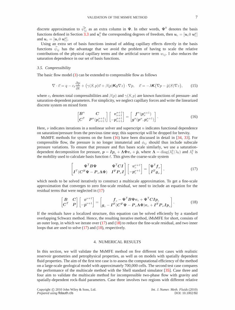
In the first test case, we evaluate the efficiency of the MsMFE solver implemented in MRST and,in particular, compare the C-accelerated version to its pure Matlab counterpart. To this end, weconsider a realistic large-scale geomodel shown in Figure3. The simulation grid is given as a asa corner-point grid with253× 258× 38 cells. After cells with zero porosity or permeability areset to be inactive, the total simulation model consists of721, 999 active cells. In addition, we haveintroduced a lower permeability threshold of 1µD. We consider a scenario in which water is injectedinto a reservoir that is initially fully oil saturated. The system is described by a standard two-phasemodel with a mobility ratio ten between the two fluids. In our timing experiments, we will focusexclusively on the pressure equation and not consider the transport solves that would normally havebeen performed on the fine scale. Our simulation setup consists of first computing basis functions,and then solving the global pressure equation one thousand times.

For multiphase flow applications, the basis functions are generally time-dependent and coupled tothe transport equation through the relative mobility termλ. For water-flooding scenarios, however,this temporal dependence is typically quite weak and good multiscale solutions can be computedusing infrequent updating of basis functions. Thinking of aBuckleyLeverett type displacementprofile, λ(x, t) will typically only vary modestly before and after the blockis swept by thedisplacement front. Favorable displacements will typically contain strong displacement fronts, andhere individual basis functions need to be updated frequently to account for large mobility variationsas the front passes through the interior of the corresponding blocks. For unfavorable displacements,as considered herein, it is often sufficient to only compute the basis functions initially [18]. To mimica worst-case scenario of mobility effects arising from saturation updates, the pressure system isreinitialized by assigning random relative permeability values to all cells before each new pressuresolve. By updating the pressure one thousand times, we get a picture of where the time is spentduring a dynamic simulation. For instance, given a pressurestep of ten days, our test will mimic asimulation of 27 years of production.

First we compare time consumption on a subset of the full geomodel. The results are displayedin TableI. The C-accelerated code gives a reduction in runtime of over80% compared to the pure



(a) (b)

Figure 3. The geomodel. The plot in (a) shows the full253 × 258 × 38 model with a15× 15× 7 coarse gridimposed. The plot in (b) shows a subset of the full model.

MATLAB implementation even though the MEX interface is not optimal since data must be copiedbetween C and MATLAB. Solving the same system on the fine scalewith the AGMG multigridsolver [37] takes 200 seconds, and hence the MsMFE solver gives a reduction of 86% in runtimecompared to the fine-scale solver for the pure Matlab solver and 97% for the C-accelerated solver.

The results for the C-accelerated code on the full geomodel are shown in TableII . For large datasets, as in this case, implementing the whole multiscale simulator in a compiled language would bemuch more efficient, since a significant computational overhead is induced when using the MEXinterface to copy data between MATLAB and C in the C-accelerated MRST code. In particular, forthe reconstruction of fine-scale fluxes, which is the most expensive operation reported in TableII ,over 50% of the time is spent copying data. Moreover, an obvious advantage of the MsMFEsolver is that it has a relatively low memory use compared e.g., with the AGMG solver, whichrequired more memory than the 4 GiB that were available on ourmeager test computer. Finally,in the simulations reported above, the basis functions werecomputed serially. Since each basisfunction can be computed independently of the other, this part of the algorithm is straightforwardto parallelize and is expected to give an almost perfect speedup. Parallelizing the reconstruction offine fluxes is a bit more complex, but should also give a significant speedup.

We expect that the results presented above extend readily toincompressibleblack-oil models inthe absence of gravity and capillary forces: the key to efficiency is to reuse basis functions from onestep to the next and exploit the natural parallelism in computing basis functions and reconstructingfine-scale fluxes.

4.2. Example 2: Carbonate sector model

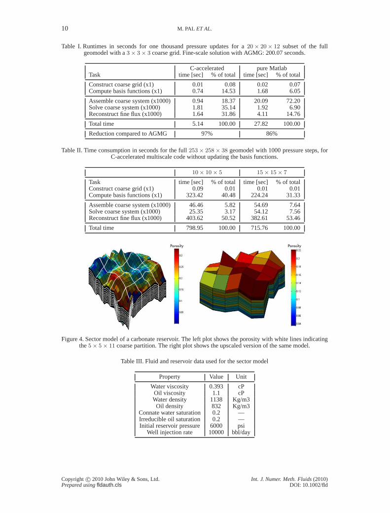
The geometrical and physical properties used in this particular sector model are based on a real-fieldcarbonate reservoir. The sector model covers a2× 2 km2 area and has a thickness of approximatelyfifty meters. The fine-scale model has20× 20 cells in the lateral direction and 93 cell layers in thevertical direction, which we partition into a coarse grid with 5× 5× 11 blocks. For comparison,we also generate a corresponding upscaled model based on a standard flow-based method. Figure4shows the fine-scale porosity distribution, the coarse partition used by the multiscale method, aswell as the upscaled model. Here, we see that unlike the upscaling method, the multiscale partitionpreserves the exact geometry of the fine-scale model.

The reservoir is produced using a five-spot injection pattern, with one injector at each corner ofthe model and one producer in the center. The fluid and the reservoir data used for the simulationsare presented in TableIII . The model represents a scenario with 2000 days of production.

In the following, we will compare four different simulationstrategies: using standard sequentialsolvers from MRST on the coarse and fine grids, using the MsMFEmethod, and using Shell’s


10 M. PAL ET AL.

Table I. Runtimes in seconds for one thousand pressure updates for a20× 20× 12 subset of the fullgeomodel with a3× 3× 3 coarse grid. Fine-scale solution with AGMG: 200.07 seconds.

C-accelerated pure MatlabTask time [sec] % of total time [sec] % of total

Construct coarse grid (x1) 0.01 0.08 0.02 0.07Compute basis functions (x1) 0.74 14.53 1.68 6.05

Assemble coarse system (x1000) 0.94 18.37 20.09 72.20Solve coarse system (x1000) 1.81 35.14 1.92 6.90Reconstruct fine flux (x1000) 1.64 31.86 4.11 14.76

Total time 5.14 100.00 27.82 100.00

Reduction compared to AGMG 97% 86%

Table II. Time consumption in seconds for the full253× 258× 38 geomodel with 1000 pressure steps, forC-accelerated multiscale code without updating the basis functions.

10× 10× 5 15× 15× 7

Task time [sec] % of total time [sec] % of totalConstruct coarse grid (x1) 0.09 0.01 0.01 0.01Compute basis functions (x1) 323.42 40.48 224.24 31.33

Assemble coarse system (x1000) 46.46 5.82 54.69 7.64Solve coarse system (x1000) 25.35 3.17 54.12 7.56Reconstruct fine flux (x1000) 403.62 50.52 382.61 53.46

Total time 798.95 100.00 715.76 100.00

Figure 4. Sector model of a carbonate reservoir. The left plot shows the porosity with white lines indicatingthe5× 5× 11 coarse partition. The right plot shows the upscaled versionof the same model.

Table III. Fluid and reservoir data used for the sector model

Property Value Unit

Water viscosity 0.393 cPOil viscosity 1.1 cPWater density 1138 Kg/m3Oil density 832 Kg/m3

Connate water saturation 0.2 —Irreducible oil saturation 0.2 —Initial reservoir pressure 6000 psi

Well injection rate 10000 bbl/day



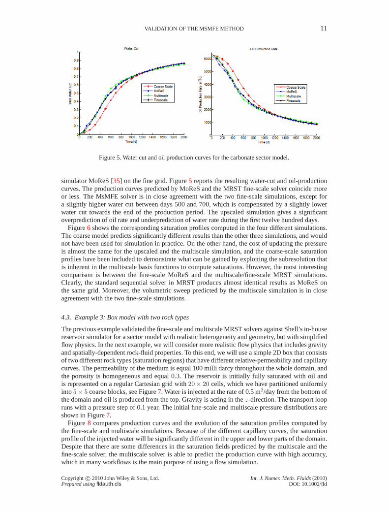
Figure 5. Water cut and oil production curves for the carbonate sector model.

simulator MoReS [35] on the fine grid. Figure5 reports the resulting water-cut and oil-productioncurves. The production curves predicted by MoReS and the MRST fine-scale solver coincide moreor less. The MsMFE solver is in close agreement with the two fine-scale simulations, except fora slightly higher water cut between days 500 and 700, which iscompensated by a slightly lowerwater cut towards the end of the production period. The upscaled simulation gives a significantoverprediction of oil rate and underprediction of water rate during the first twelve hundred days.

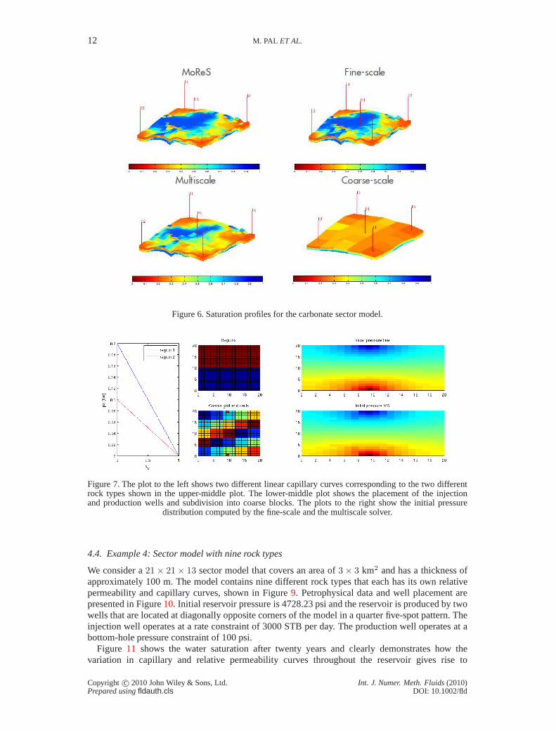
Figure6 shows the corresponding saturation profiles computed in thefour different simulations.The coarse model predicts significantly different results than the other three simulations, and wouldnot have been used for simulation in practice. On the other hand, the cost of updating the pressureis almost the same for the upscaled and the multiscale simulation, and the coarse-scale saturationprofiles have been included to demonstrate what can be gainedby exploiting the subresolution thatis inherent in the multiscale basis functions to compute saturations. However, the most interestingcomparison is between the fine-scale MoReS and the multiscale/fine-scale MRST simulations.Clearly, the standard sequential solver in MRST produces almost identical results as MoReS onthe same grid. Moreover, the volumetric sweep predicted by the multiscale simulation is in closeagreement with the two fine-scale simulations.

4.3. Example 3: Box model with two rock types

The previous example validated the fine-scale and multiscale MRST solvers against Shell’s in-housereservoir simulator for a sector model with realistic heterogeneity and geometry, but with simplifiedflow physics. In the next example, we will consider more realistic flow physics that includes gravityand spatially-dependent rock-fluid properties. To this end, we will use a simple 2D box that consistsof two different rock types (saturation regions) that have different relative-permeability and capillarycurves. The permeability of the medium is equal 100 milli darcy throughout the whole domain, andthe porosity is homogeneous and equal 0.3. The reservoir is initially fully saturated with oil andis represented on a regular Cartesian grid with20× 20 cells, which we have partitioned uniformlyinto 5× 5 coarse blocks, see Figure7. Water is injected at the rate of 0.5 m2/day from the bottom ofthe domain and oil is produced from the top. Gravity is actingin thez-direction. The transport loopruns with a pressure step of 0.1 year. The initial fine-scale and multiscale pressure distributions areshown in Figure7.

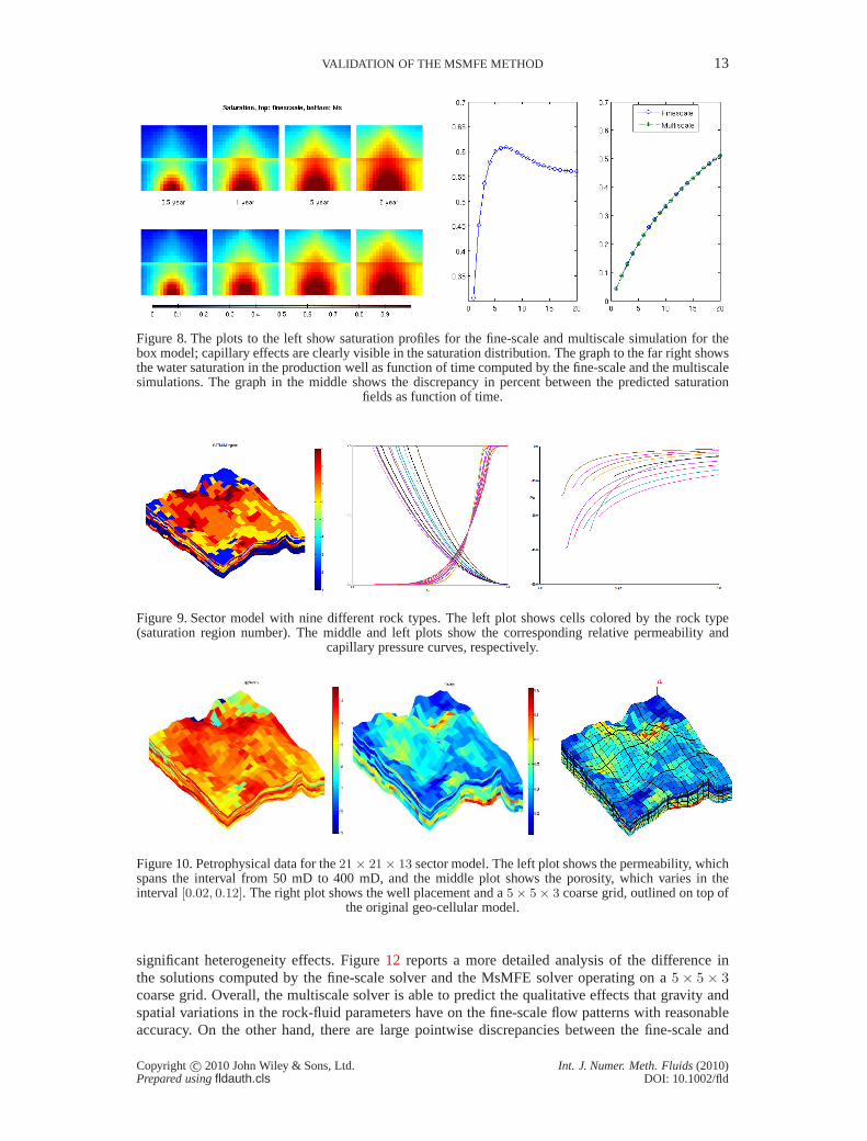
Figure8 compares production curves and the evolution of the saturation profiles computed bythe fine-scale and multiscale simulations. Because of the different capillary curves, the saturationprofile of the injected water will be significantly differentin the upper and lower parts of the domain.Despite that there are some differences in the saturation fields predicted by the multiscale and thefine-scale solver, the multiscale solver is able to predict the production curve with high accuracy,which in many workflows is the main purpose of using a flow simulation.


12 M. PAL ET AL.

Figure 6. Saturation profiles for the carbonate sector model.

Figure 7. The plot to the left shows two different linear capillary curves corresponding to the two differentrock types shown in the upper-middle plot. The lower-middleplot shows the placement of the injectionand production wells and subdivision into coarse blocks. The plots to the right show the initial pressure

distribution computed by the fine-scale and the multiscale solver.

4.4. Example 4: Sector model with nine rock types

We consider a21× 21× 13 sector model that covers an area of3× 3 km2 and has a thickness ofapproximately 100 m. The model contains nine different rocktypes that each has its own relativepermeability and capillary curves, shown in Figure9. Petrophysical data and well placement arepresented in Figure10. Initial reservoir pressure is 4728.23 psi and the reservoir is produced by twowells that are located at diagonally opposite corners of themodel in a quarter five-spot pattern. Theinjection well operates at a rate constraint of 3000 STB per day. The production well operates at abottom-hole pressure constraint of 100 psi.

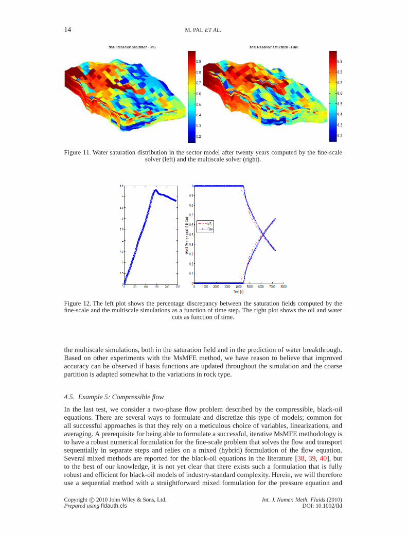
Figure 11 shows the water saturation after twenty years and clearly demonstrates how thevariation in capillary and relative permeability curves throughout the reservoir gives rise to



Figure 8. The plots to the left show saturation profiles for the fine-scale and multiscale simulation for thebox model; capillary effects are clearly visible in the saturation distribution. The graph to the far right showsthe water saturation in the production well as function of time computed by the fine-scale and the multiscalesimulations. The graph in the middle shows the discrepancy in percent between the predicted saturation

fields as function of time.

Figure 9. Sector model with nine different rock types. The left plot shows cells colored by the rock type(saturation region number). The middle and left plots show the corresponding relative permeability and

capillary pressure curves, respectively.

Figure 10. Petrophysical data for the21× 21× 13 sector model. The left plot shows the permeability, whichspans the interval from 50 mD to 400 mD, and the middle plot shows the porosity, which varies in theinterval [0.02, 0.12]. The right plot shows the well placement and a5× 5× 3 coarse grid, outlined on top of

the original geo-cellular model.

significant heterogeneity effects. Figure12 reports a more detailed analysis of the difference inthe solutions computed by the fine-scale solver and the MsMFEsolver operating on a5× 5× 3coarse grid. Overall, the multiscale solver is able to predict the qualitative effects that gravity andspatial variations in the rock-fluid parameters have on the fine-scale flow patterns with reasonableaccuracy. On the other hand, there are large pointwise discrepancies between the fine-scale and


14 M. PAL ET AL.

Figure 11. Water saturation distribution in the sector model after twenty years computed by the fine-scalesolver (left) and the multiscale solver (right).

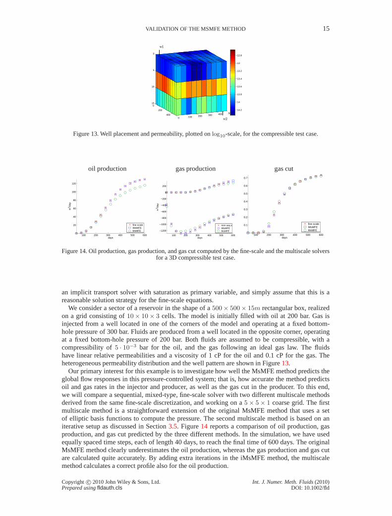
Figure 12. The left plot shows the percentage discrepancy between the saturation fields computed by thefine-scale and the multiscale simulations as a function of time step. The right plot shows the oil and water

cuts as function of time.

the multiscale simulations, both in the saturation field andin the prediction of water breakthrough.Based on other experiments with the MsMFE method, we have reason to believe that improvedaccuracy can be observed if basis functions are updated throughout the simulation and the coarsepartition is adapted somewhat to the variations in rock type.

4.5. Example 5: Compressible flow

In the last test, we consider a two-phase flow problem described by the compressible, black-oilequations. There are several ways to formulate and discretize this type of models; common forall successful approaches is that they rely on a meticulous choice of variables, linearizations, andaveraging. A prerequisite for being able to formulate a successful, iterative MsMFE methodology isto have a robust numerical formulation for the fine-scale problem that solves the flow and transportsequentially in separate steps and relies on a mixed (hybrid) formulation of the flow equation.Several mixed methods are reported for the black-oil equations in the literature [38, 39, 40], butto the best of our knowledge, it is not yet clear that there exists such a formulation that is fullyrobust and efficient for black-oil models of industry-standard complexity. Herein, we will thereforeuse a sequential method with a straightforward mixed formulation for the pressure equation and



0

200

4000 100 200 300 400 500

0

5

10

15

w2

w1

−14.2

−14

−13.8

−13.6

−13.4

−13.2

−13

−12.8

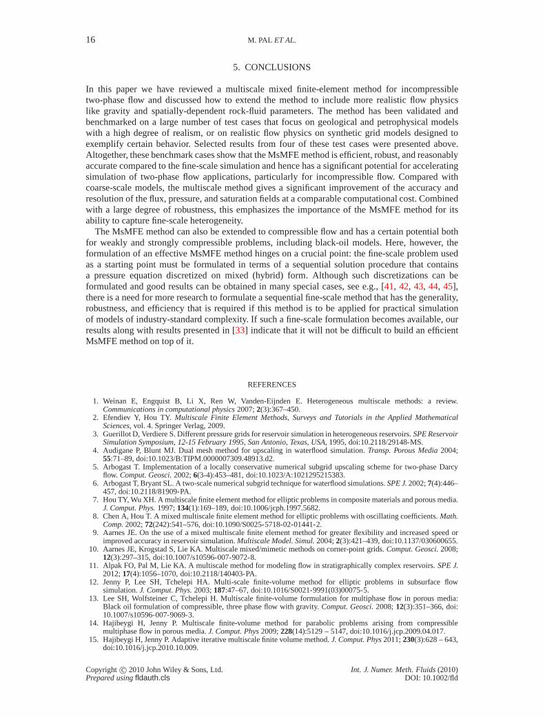
Figure 13. Well placement and permeability, plotted onlog10-scale, for the compressible test case.

oil production gas production gas cut

100 200 300 400 500 600

20

40

60

80

100

120

days

m3 /d

ay

fine scaleiMsMFEMsMFE

100 200 300 400 500 600

−1200

−1000

−800

−600

−400

−200

0

200

days

m3 /d

ay

mim seq siMsMFEMsMFE

100 200 300 400 500 600

0.1

0.2

0.3

0.4

0.5

0.6

0.7

days

fine scaleiMsMFEMsMFE

Figure 14. Oil production, gas production, and gas cut computed by the fine-scale and the multiscale solversfor a 3D compressible test case.

an implicit transport solver with saturation as primary variable, and simply assume that this is areasonable solution strategy for the fine-scale equations.

We consider a sector of a reservoir in the shape of a500× 500× 15m rectangular box, realizedon a grid consisting of10× 10× 3 cells. The model is initially filled with oil at 200 bar. Gas isinjected from a well located in one of the corners of the modeland operating at a fixed bottom-hole pressure of 300 bar. Fluids are produced from a well located in the opposite corner, operatingat a fixed bottom-hole pressure of 200 bar. Both fluids are assumed to be compressible, with acompressibility of5 · 10−3 bar for the oil, and the gas following an ideal gas law. The fluidshave linear relative permeabilities and a viscosity of 1 cP for the oil and 0.1 cP for the gas. Theheterogeneous permeability distribution and the well pattern are shown in Figure13.

Our primary interest for this example is to investigate how well the MsMFE method predicts theglobal flow responses in this pressure-controlled system; that is, how accurate the method predictsoil and gas rates in the injector and producer, as well as the gas cut in the producer. To this end,we will compare a sequential, mixed-type, fine-scale solverwith two different multiscale methodsderived from the same fine-scale discretization, and working on a5× 5× 1 coarse grid. The firstmultiscale method is a straightforward extension of the original MsMFE method that uses a setof elliptic basis functions to compute the pressure. The second multiscale method is based on aniterative setup as discussed in Section3.5. Figure14 reports a comparison of oil production, gasproduction, and gas cut predicted by the three different methods. In the simulation, we have usedequally spaced time steps, each of length 40 days, to reach the final time of 600 days. The originalMsMFE method clearly underestimates the oil production, whereas the gas production and gas cutare calculated quite accurately. By adding extra iterations in the iMsMFE method, the multiscalemethod calculates a correct profile also for the oil production.


16 M. PAL ET AL.

5. CONCLUSIONS

In this paper we have reviewed a multiscale mixed finite-element method for incompressibletwo-phase flow and discussed how to extend the method to include more realistic flow physicslike gravity and spatially-dependent rock-fluid parameters. The method has been validated andbenchmarked on a large number of test cases that focus on geological and petrophysical modelswith a high degree of realism, or on realistic flow physics on synthetic grid models designed toexemplify certain behavior. Selected results from four of these test cases were presented above.Altogether, these benchmark cases show that the MsMFE method is efficient, robust, and reasonablyaccurate compared to the fine-scale simulation and hence hasa significant potential for acceleratingsimulation of two-phase flow applications, particularly for incompressible flow. Compared withcoarse-scale models, the multiscale method gives a significant improvement of the accuracy andresolution of the flux, pressure, and saturation fields at a comparable computational cost. Combinedwith a large degree of robustness, this emphasizes the importance of the MsMFE method for itsability to capture fine-scale heterogeneity.

The MsMFE method can also be extended to compressible flow andhas a certain potential bothfor weakly and strongly compressible problems, including black-oil models. Here, however, theformulation of an effective MsMFE method hinges on a crucialpoint: the fine-scale problem usedas a starting point must be formulated in terms of a sequential solution procedure that containsa pressure equation discretized on mixed (hybrid) form. Although such discretizations can beformulated and good results can be obtained in many special cases, see e.g., [41, 42, 43, 44, 45],there is a need for more research to formulate a sequential fine-scale method that has the generality,robustness, and efficiency that is required if this method isto be applied for practical simulationof models of industry-standard complexity. If such a fine-scale formulation becomes available, ourresults along with results presented in [33] indicate that it will not be difficult to build an efficientMsMFE method on top of it.

REFERENCES

1. Weinan E, Engquist B, Li X, Ren W, Vanden-Eijnden E. Heterogeneous multiscale methods: a review.Communications in computational physics2007;2(3):367–450.

2. Efendiev Y, Hou TY.Multiscale Finite Element Methods, Surveys and Tutorials in the Applied MathematicalSciences, vol. 4. Springer Verlag, 2009.

3. Guerillot D, Verdiere S. Different pressure grids for reservoir simulation in heterogeneous reservoirs.SPE ReservoirSimulation Symposium, 12-15 February 1995, San Antonio, Texas, USA, 1995, doi:10.2118/29148-MS.

4. Audigane P, Blunt MJ. Dual mesh method for upscaling in waterflood simulation.Transp. Porous Media2004;55:71–89, doi:10.1023/B:TIPM.0000007309.48913.d2.

5. Arbogast T. Implementation of a locally conservative numerical subgrid upscaling scheme for two-phase Darcyflow. Comput. Geosci.2002;6(3-4):453–481, doi:10.1023/A:1021295215383.

6. Arbogast T, Bryant SL. A two-scale numerical subgrid technique for waterflood simulations.SPE J.2002;7(4):446–457, doi:10.2118/81909-PA.

7. Hou TY, Wu XH. A multiscale finite element method for elliptic problems in composite materials and porous media.J. Comput. Phys.1997;134(1):169–189, doi:10.1006/jcph.1997.5682.

8. Chen A, Hou T. A mixed multiscale finite element method for elliptic problems with oscillating coefficients.Math.Comp.2002;72(242):541–576, doi:10.1090/S0025-5718-02-01441-2.

9. Aarnes JE. On the use of a mixed multiscale finite element method for greater flexibility and increased speed orimproved accuracy in reservoir simulation.Multiscale Model. Simul.2004;2(3):421–439, doi:10.1137/030600655.

10. Aarnes JE, Krogstad S, Lie KA. Multiscale mixed/mimeticmethods on corner-point grids.Comput. Geosci.2008;12(3):297–315, doi:10.1007/s10596-007-9072-8.

11. Alpak FO, Pal M, Lie KA. A multiscale method for modeling flow in stratigraphically complex reservoirs.SPE J.2012;17(4):1056–1070, doi:10.2118/140403-PA.

12. Jenny P, Lee SH, Tchelepi HA. Multi-scale finite-volume method for elliptic problems in subsurface flowsimulation.J. Comput. Phys.2003;187:47–67, doi:10.1016/S0021-9991(03)00075-5.

13. Lee SH, Wolfsteiner C, Tchelepi H. Multiscale finite-volume formulation for multiphase flow in porous media:Black oil formulation of compressible, three phase flow withgravity. Comput. Geosci.2008;12(3):351–366, doi:10.1007/s10596-007-9069-3.

14. Hajibeygi H, Jenny P. Multiscale finite-volume method for parabolic problems arising from compressiblemultiphase flow in porous media.J. Comput. Phys2009;228(14):5129 – 5147, doi:10.1016/j.jcp.2009.04.017.

15. Hajibeygi H, Jenny P. Adaptive iterative multiscale finite volume method.J. Comput. Phys2011;230(3):628 – 643,doi:10.1016/j.jcp.2010.10.009.



16. Møyner O, Lie KA. The multiscale finite-volume method on stratigraphic grids.SPE J.2014; doi:10.2118/163649-PA.

17. Møyner O, Lie KA. A multiscale two-point flux-approximation method.J. Comput. Phys.2014; .18. Kippe V, Aarnes JE, Lie KA. A comparison of multiscale methods for elliptic problems in porous media flow.

Comput. Geosci.2008;12(3):377–398, doi:10.1007/s10596-007-9074-6.19. Farmer CL. Upscaling: a review.Int. J. Numer. Meth. Fluids2002;40(1–2):63–78, doi:10.1002/fld.267.20. Durlofsky LJ. Upscaling and gridding of fine scale geological models for flow simulation 2005. Presented at 8th

International Forum on Reservoir Simulation Iles Borromees, Stresa, Italy, June 20–24, 2005.21. The MATLAB Reservoir Simulation Toolbox, version 2011bJan 2012.http://www.sintef.no/MRST/.22. Wheeler MF. Mimetic finite difference methods for flow in porous media.Center for subsurface modeling industrial

affiliates meeting, oct. 21–22, University of Texas, Austin 2003.23. Brezzi F, Lipnikov K, Simoncini V. A family of mimetic finite difference methods on polygonial and polyhedral

meshes.Math. Models Methods Appl. Sci.2005;15:1533–1553, doi:10.1142/S0218202505000832.24. Brezzi F, Lipnikov K, Shashkov M, Simoncini V. A new dicretization methodology for diffusion problems on

generalized polyhedral meshes 2005. LAUR-05-8717, Report.25. Aavatsmark I. An introduction to multipoint flux approximations for quadrilateral grids.Comput. Geosci.2002;

6:405–432, doi:10.1023/A:1021291114475.26. Edwards MG, Rogers CF. Finite volume discretization with imposed flux continuity for the general tensor pressure

equation.Comput. Geosci.1998;2:259–290. 10.1023/A:1011510505406.27. Pal M, Edwards MG, Lamb AR. Convergence study of a family of flux-continuous, finite-volume schemes

for the general tensor pressure equation.Internat. J. Numer. Methods Fluids2006; 51(9-10):1177–1203, doi:10.1002/fld.1211.

28. Lamine S, Edwards MG. Higher order multidimensional wave oriented upwind schemes for flow in porous mediaon unstructured grids.SPE Reservoir Simulation Symposium, The Woodlands, TX, USA, 2–4 February 2009, 2009,doi:10.2118/119187-MS.

29. Lamine S, Edwards MG. Higher order multidimensional upwind convection schemes for flow in porous mediaon structured and unstructured quadrilateral grids.SIAM J. Sci. Comput.2010; 32(3):1119–1139, doi:10.1137/080727750.

30. Natvig JR, Skaflestad B, Bratvedt F, Bratvedt K, Lie KA, Laptev V, Khataniar SK. Multiscale mimetic solvers forefficient streamline simulation of fractured reservoirs.SPE J.2011;16(4), doi:10.2018/119132-PA.

31. Lie KA, Natvig JR, Krogstad S, Yang Y, Wu XH. Grid adaptation for the Dirichlet–Neumann representation methodand the multiscale mixed finite-element method.Comput. Geosci.2014; doi:10.1007/s10596-013-9397-4.

32. Aarnes JE, Krogstad S, Lie KA. A hierarchical multiscalemethod for two-phase flow based upon mixed finiteelements and nonuniform coarse grids.Multiscale Model. Simul.2006;5(2):337–363, doi:10.1137/050634566.

33. Krogstad S, Lie KA, Skaflestad B. Mixed multiscale methods for compressible flow.Proceedings of ECMOR XIII–13th European Conference on the Mathematics of Oil Recovery, EAGE: Biarritz, France, 2012.

34. Krogstad S. A sparse basis POD for model reduction of multiphase compressible flow.2011 SPE ReservoirSimulation Symposium, The Woodlands, Texas, USA, 21-23 February 2011, 2011, doi:10.2118/141973-MS.

35. MoReS. Shell’s Reservoir Simulation Toolbox, version 2010.http://www.shell.com February 2010.36. Lie K, Krogstad S, Ligaarden I, Natvig J, Nilsen H, Skaflestad B. Open-source MATLAB implementation of

consistent discretisations on complex grids.Comput. Geosci.2012;16:297–322. 10.1007/s10596-011-9244-4.37. Notay Y. An aggregation-based algebraic multigrid method.Electron. Trans. Numer. Anal.2010;37:123–140.38. Bergamaschi L, Mantica S, Manzini G. A mixed finite element–finite volume formulation of the black-oil model.

SIAM Journal on Scientific Computing1998;20(3):970–997, doi:10.1137/S1064827595289303.39. Chen Z. Formulations and numerical methods of the black oil model in porous media.SIAM J. Numer. Anal.Jul

2000;38(2):489–514, doi:10.1137/S0036142999304263.40. Krogstad S, Lie KA, Nilsen HM, Natvig JR, Skaflestad B, Aarnes JE. A multiscale mixed finite-element solver for

three-phase black-oil flow.SPE Reservoir Simulation Symposium, The Woodlands, TX, USA, 2–4 February 2009,2009, doi:10.2118/118993-MS.

41. Bergamaschi L, Mantica S, Manzini G. A mixed finite element-finite volume formulation of the black-oil model.SIAM J. Sci. Comput1998;20(3):970–997, doi:10.1137/S1064827595289303.

42. Chen Z. Formulations and numerical methods of the black oil model in porous media.SIAM J. Numer. Anal.2000;38(2):489–514, doi:10.1137/S0036142999304263.

43. Yang D. A splitting positive definite mixed element method for miscible displacement of compressible flow inporous media.Numer. Methods Partial Differential Equations2001;17(3):229–249, doi:10.1002/num.3.

44. Cui M. A combined mixed and discontinuous galerkin method for compressible miscible displacement problem inporous media.J. Comput. Appl. Math.2007;198(1):19–34, doi:10.1016/j.cam.2005.11.021.

45. Yang Jm, Chen Y. Superconvergence of a combined mixed finite element and discontinuous Galerkin methodfor a compressible miscible displacement problem.Acta Math. Appl. Sin.2011; 27(3):481–494, doi:10.1007/s10255-011-0081-y.


Validation of the multiscale mixed ﬁnite-element method

Documents

Transcript of Validation of the multiscale mixed ﬁnite-element method