Error analysis of finite element and finite volume

methods for some viscoelastic fluids

Maria Lukacova-Medvid’ova∗, Hana Mizerova∗, Bangwei She∗,

Jan Stebel†

Abstract

We present the error analysis of a particular Oldroyd-B type modelwith the limiting Weissenberg number going to infinity. Assuming a suit-able regularity of the exact solution we study the error estimates of astandard finite element method and of a combined finite element/finitevolume method. Our theoretical result shows first order convergence ofthe finite element method and the error of the order O(h3/4) for the finiteelement/finite volume method. These error estimates are compared andconfirmed by the numerical experiments.

Keywords: error analysis, Oldroyd-B type models, viscoelastic fluids, finite el-ement method, finite volume method, finite difference method, highWeissenbergnumber, multiplicative trace inequality

1 Introduction

Many biological, industrial or geological fluids can no longer be described bya linear relation between the stress and the deformation tensor. These com-plex fluids fall into a class of the so-called non-Newtonian fluids. Recently, anincreasing number of mathematicians have become interested in mathematicalmodeling and numerical simulation of complex fluids and there exists already arich body of literature on mathematical analysis and problem-suited numericalmethods. Mathematical models consist of the conservation laws describing theconservation of mass (div-free condition for the velocity vector) and momentum.The stress tensor is typically written as a sum of viscous stress tensor dependinglinearly on the deformation tensor and the extra stress due to the polymer con-tribution. In macroscopic models the latter is given by a complex constitutive

∗Institute of Mathematics, University of Mainz, Staudingerweg 9, 55099 Mainz, Ger-

many,lukacova,mizerova,bangwei@uni-mainz.de†Institute of Mathematics AS CR, Zitna 25, 110 00 Praha, Czech Republic,

stebel@math.cas.cz

1

equation to capture the corresponding viscoelastic properties. In order to de-scribe the evolution of viscoelastic stress tensor various approaches can be used.Let us mention, for example, differential, integral models or macro-micro modelsbased on the kinetic formulation of the probability distribution function. Well-known differential models are the Oldroyd-B or the Johnson-Segelman models,where an additional transport equation is added to describe the time evolu-tion of the polymer stress tensor. In what follows we will concentrate on thedifferential viscoelastic models.

In the mathematical literature we can find already various results dealingwith the questions of well-posedness of the viscoelastic flows and in particularwith the Oldroyd-B model. Let us mention classical results on strong solutionspublished by Fernandez-Cara, Guillen and Ortega [14] and of Guillope and Saut[16], see also [18] for further related results on the existence of strong solutionsin exterior domains obtained by Hieber, Naito and Shibata.

Recently, the global existence result for fully two- and three-dimensional flowhas been obtained by Lions and Masmoudi [24] for the case of the co-rotationalOldroyd model. In [23] the local existence of solutions and global existence ofsmall solutions of some rate type fluids have been shown, global existence ofweak solutions for small data can be found, e.g., in [8]. In the recent work[1] Barrett and Boyaval studied the so-called diffusive Oldroyd-B model bothfrom numerical as well as analytical point of view. For two space dimensionsthey were able to prove the global existence of weak solutions. The diffusiveOldroyd-B model has also been studied by Constantin and Kliegl in [7] and theglobal regularity in two space dimensions has been proven.

Concerning numerical simulation of the Oldroyd-B type flows a major obsta-cle is the high Weissenberg number problem. The so-called numerical blow-upis a widely known phenomenon in numerical simulations of high Weissenbergnumber viscoelastic flows. It is anticipated that the blow-up has various rea-sons: influence of domain singularities, missing analytical results on the well-posedness of global weak solutions and numerical instabilities. The latter isa purely numerical phenomenon that arises due to the inadequacy of polyno-mial interpolations to approximate spatial exponential profiles, which is thecase of the elastic stress tensor. In [13] a new promising approach using thelog-conformation tensor has been proposed, see also further related works [5],[2], [10] and the references therein.

In this paper we consider the following viscoelastic model that can be achievedas a limiting case of the Oldroyd-B model when the relaxation time goes to in-finity. Note that this assumption is equivalent to the fact that the Weissenbergnumber We, which is a non-dimensional parameter expressing a ratio of therelaxation time to a typical flow time scale, is set to infinity.

∂tu+ div(u ⊗ u)− ν∆u+∇π = div(FF>) (1a)

divu = 0 (1b)

∂tF+ (u · ∇)F = (∇u)F (1c)

Indeed, when setting the elastic part of the stress tensor Te = FFT we recover

2

the Oldroyd-B model with We → ∞. Consequently, the transport equation forthe elastic stress Te reads

∂tTe + (u · ∇)Te − (∇u)Te − T

e(∇u)T = 0.

The system (1a)–(1c) describes the unsteady motion of a viscoelastic fluidin a bounded domain Ω ⊂ R

2 with sufficiently smooth boundary in the timeinterval (0, T ) and is complemented with the no-slip boundary condition

u|∂Ω = 0 (1d)

and the initial conditions

u(0, ·) = u0, F(0, ·) = F0. (1e)

The viscosity ν > 0 is assumed to be constant. Note that there is no needto prescribe the boundary condition for F since (1c) is a first-order transportequation and u = 0 on the boundary.

We should mention that the question of global in time existence of weaksolutions of (1) is still open. Local existence of strong solutions has been provenin [20], [23] as well as in [6]. As far as we know this model has not yet beenstudied from the numerical point of view and our paper is the first contributionin this direction. More interestingly, we would like to point out that we donot need any particular stabilization techniques for high Weissenberg numberproblems and obtain stable and convergent results using some suitable numericalapproximations that are typically used in computational fluid dynamics.

The main aim of this paper is to present error analysis of two finite element-type approximations of the problem (1). In particular, we combine the low-est order Taylor-Hood finite element discretization of the flow part (piecewisequadratic velocity and piecewise linear pressure) with either piecewise linearfinite elements or finite volumes for the deformation gradient. The paper isorganized as follows. In Section 2 we introduce space discretizations of (1). Themain result on convergence rates is stated in Section 3. Sections 4 and 5 aredevoted to the proof of the main result. In the second part of the proof we usea variant of the multiplicative trace inequality, which is proved in Section 6.Finally, we present results of a numerical test in Section 7.

2 Approximation

Before passing to the finite dimensional approximation, let us introduce the basicnotation. Throughout the paper we shall use the space Ck(B) of continuously k-times differentiable functions in an compact set B, the Lebesgue space Lp(Ω), itssubspace Lp

0(Ω) of functions with zero integral mean, the Sobolev spaceW k,p(Ω)and the Sobolev space W 1,p

0 (Ω) of functions with vanishing trace. Lebesgueand Sobolev spaces with values in some Banach space X will be denoted by

3

Lp(Ω;X), W k,p(Ω;X), respectively. The norm in Lp(Ω) and W k,p(Ω) will bedenoted ‖ · ‖p, ‖ · ‖k,p, respectively. We shall employ the continuous embeddings

W 1,p(Ω) → L2p

2−p (Ω), W 2,2(Ω) → L∞(Ω) (2)

and the Sobolev inequality

∀v ∈ W 1,20 (Ω) : ‖v‖24 ≤ C‖v‖2‖∇v‖2. (3)

Here and in what follows, C will stand for a generic positive constant whosevalue may change from line to line. If fg ∈ L1(Ω) then we shall write (f, g)in place of

∫

Ω fg. The following variant of Young’s inequality holds: For everyp ∈ (1,∞) there exists C = C(p) > 0 such that ∀α > 0, f ∈ Lp(Ω), g ∈ Lq(Ω):

(f, g) ≤ α

∫

Ω

|f |p + Cα− q

p

∫

Ω

|g|q, (4)

where q = p/(p− 1).Let Thh>0 be a family of partitions of Ω into triangles and h be the length

of the largest edge in Th. For any T ∈ Th and k = 0, 1, 2, . . . we denote by Pk(T )the space of k-th degree polynomials on T . We define the spaces

Wh := v ∈ W 1,20 (Ω;R2); ∀T ∈ Th : v|T ∈ P2(T )2,

Lh := q ∈ L20(Ω) ∩ C(Ω); ∀T ∈ Th : q|T ∈ P1(T ),

Xh := G ∈ C(Ω;R2×2); ∀T ∈ Th : G|T ∈ P1(T )2×2,

Zh := G ∈ L2(Ω;R2×2); ∀T ∈ Th : G|T ∈ P0(T ).

Let e be an interior edge shared by elements T1 and T2. Define the unitnormal vectors n1 and n2 on e pointing exterior to T1 and T2, respectively. Fora function ϕ, piecewise smooth on Th, with ϕi = ϕ|Ti

we define the average ϕand the jump [ϕ] :

ϕ =1

2(ϕ1 + ϕ2), [ϕ] = ϕ1n1 + ϕ2n2 on e ∈ E0

h,

where E0h is the set of all interior edges. For a vector-valued function φ, piecewise

smooth on Th, we define the average and the jump analogously

φ =1

2(φ1 + φ2), [φ] = φ1 · n1 + φ2 · n2 on e ∈ E0

h.

Let β be a vector-valued function, continuous across e. The upwind value of aquantity βϕ is defined as follows:

βϕu =

βϕ1 if β · n1 > 0,

βϕ2 if β · n1 < 0,

βϕ if β · n1 = 0.

We introduce the following space semi-discretizations of (1).

4

A. Finite element approximation. Find (uh, πh,Fh) ∈ C1([0, T ];Wh) ×C([0, T ];Lh)× C1([0, T ];Xh) such that

• for all (vh, qh,Gh) ∈ Wh × Lh ×Xh and t ∈ (0, T ) the following integralidentities hold:

(∂tuh(t),vh)− (uh(t)⊗ uh(t),∇vh)−1

2((divuh(t))uh(t),vh)

+ ν(∇uh(t),∇vh)− (πh(t), div vh) + (Fh(t)F>h (t),∇vh) = 0, (5a)

(qh, divuh(t)) = 0, (5b)

(∂tFh(t),Gh)− ((uh(t) · ∇)Gh,Fh(t))−1

2((divuh(t))Fh(t),Gh)

− ((∇uh(t))Fh(t),Gh) = 0; (5c)

• uh and Fh satisfy the initial conditions: for all vh ∈ Wh and Gh ∈ Xh

(uh(0, ·),vh) = (u0,vh), (Fh(0, ·),Gh) = (F0,Gh). (6)

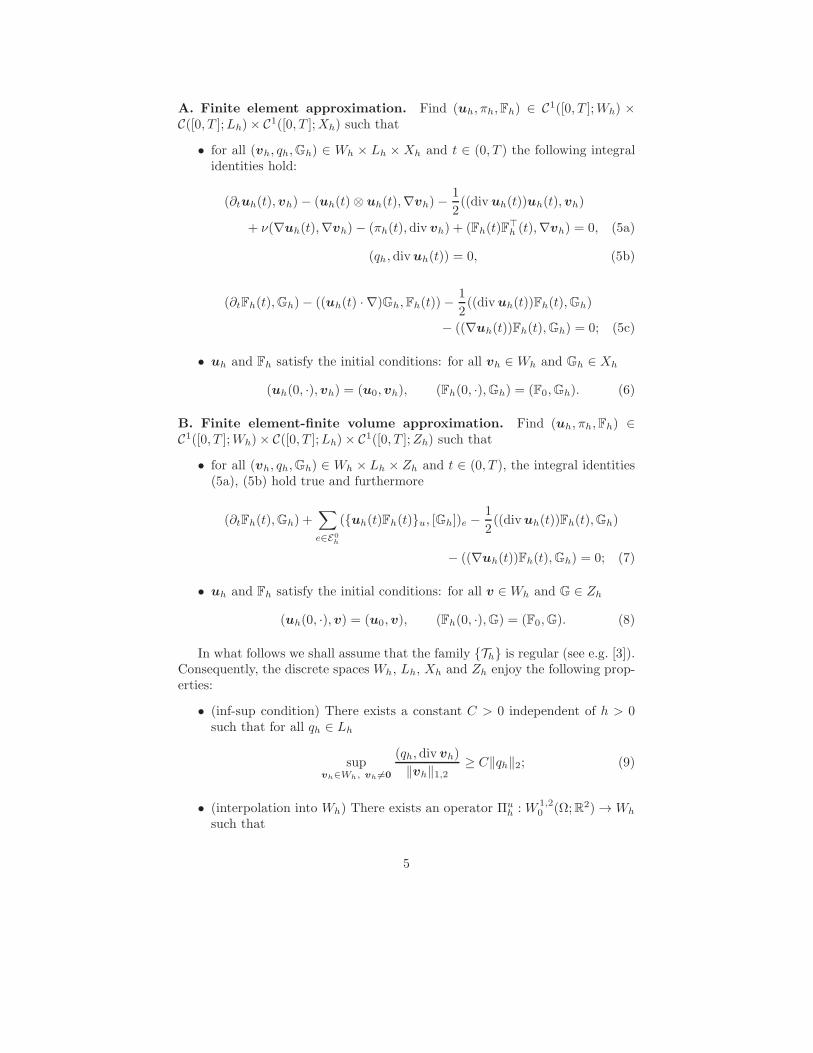
B. Finite element-finite volume approximation. Find (uh, πh,Fh) ∈C1([0, T ];Wh)× C([0, T ];Lh)× C1([0, T ];Zh) such that

• for all (vh, qh,Gh) ∈ Wh × Lh × Zh and t ∈ (0, T ), the integral identities(5a), (5b) hold true and furthermore

(∂tFh(t),Gh) +∑

e∈E0

h

(uh(t)Fh(t)u, [Gh])e −1

2((divuh(t))Fh(t),Gh)

− ((∇uh(t))Fh(t),Gh) = 0; (7)

• uh and Fh satisfy the initial conditions: for all v ∈ Wh and G ∈ Zh

(uh(0, ·),v) = (u0,v), (Fh(0, ·),G) = (F0,G). (8)

In what follows we shall assume that the family Th is regular (see e.g. [3]).Consequently, the discrete spaces Wh, Lh, Xh and Zh enjoy the following prop-erties:

• (inf-sup condition) There exists a constant C > 0 independent of h > 0such that for all qh ∈ Lh

supvh∈Wh, vh 6=0

(qh, div vh)

‖vh‖1,2≥ C‖qh‖2; (9)

• (interpolation into Wh) There exists an operator Πuh : W 1,2

0 (Ω;R2) → Wh

such that

5

– for all v ∈ W 1,20 (Ω;R2) ∩ W k,q(Ω;R2), 1 ≤ q ≤ ∞, k ∈ 1, 2, 3,

r ∈ 0, . . . , k:‖Πu

hv − v‖r,q ≤ Chk−r‖v‖k,q, (10)

where C > 0 is independent of h > 0;

– for all v ∈ W 1,20 (Ω;R2) and qh ∈ Lh:

(qh, div Πuhv) = (qh, div v); (11)

• (interpolation into Lh) There exists an operator Ππh : L2

0(Ω) → Lh and aconstant C > 0 independent of h > 0, such that

‖Ππhs− s‖r,q ≤ Ch2−r‖s‖2,q (12)

for all s ∈ L20(Ω) ∩W 2,q(Ω), 1 ≤ q ≤ ∞, r ∈ 0, 1;

• (interpolation into Xh) There exists an operator ΠFh : L2(Ω;R2×2) → Xh

and a constant C > 0 independent of h > 0, such that

‖ΠFhG−G‖r,q ≤ Ch2−r‖G‖2,q, (13)

for all G ∈ W 2,q(Ω;R2×2), 1 ≤ q ≤ ∞, r ∈ 0, 1.

• (interpolation into Zh) There exists an operator Π0h : L2(Ω;R2×2) → Zh

and a constant C > 0 independent of h > 0, such that

‖Π0hG−G‖q ≤ Ch‖G‖1,q, (14)

for all G ∈ W 1,q(Ω;R2×2), 1 ≤ q ≤ ∞.

The inequality (9) is the Babuska-Brezzi condition for the Taylor-Hood finite el-ement (see e.g. [4]), (10)-(14) are standard properties of interpolation operators[3].

In the error analysis of the finite element-finite volume scheme we will needthe following variant of multiplicative trace inequality.

Lemma 1. Let F ∈ W 2,2(Ω). Then there exists a constant c > 0 independentof h such that

∑

e∈E0

h

‖F −Π0hF‖4,e ≤ ch3/4‖F‖2,2. (15)

The proof of this statement is postponed to Section 6.For initial data of the form

F0 = ∇×Φ0, ∇Φ0 ∈ W k,2(Ω), u0 ∈ W k,2(Ω), k ≥ 2, (16)

it has been proved [23, Theorem 2.2] that there exists a positive time T , whichdepends only on ‖∇Φ0‖2,2 and ‖u0‖2,2, such that the system (1) possesses aunique solution in the time interval [0, T ] with

∂jt∇

αu ∈ L∞(0, T ;W k−2j−|α|,2(Ω)) ∩ L2(0, T ;W k−2j−|α|+1,2(Ω)),

∂jt∇

αF ∈ L∞(0, T ;W k−2j−|α|,2(Ω)),

(17)

6

for all j and α satisfying 2j + |α| ≤ k.For the approximate problems we have the following result.

Lemma 2. Let T > 0, u0 ∈ L2(Ω;R2) and F0 ∈ L2(Ω;R2×2). Then there existsh0 > 0 such that for every h ∈ (0, h0) problem A (or problem B, respectively)has a unique global in time solution (uh, πh,Fh), which satisfies

‖uh(τ, ·)‖22 + ‖Fh(τ, ·)‖

22 + 2ν

∫ τ

0

‖∇uh‖22 = ‖u0‖

22 + ‖F0‖

22 (18)

for all τ ∈ (0, T ).

Proof. A semidiscrete systems (5) or (5a), (5b), (7) and (8) yield the systemof ordinary differential equations, whose solution can be proven applying thestandard arguments for the ordinary differential systems and showing the aprioriestimates (18) following [23].

3 Main result

Now let us state the main result on the error rates.

Theorem 1. Let the family Thh>0 be regular, the initial data (u0,∇× Φ0)satisfy u0,∇Φ0 ∈ W 2,2(Ω) and [0, T ] be the maximal time interval in which thestrong solution (u, π,F) to (1) exists. Then there exist constants h0 > 0 andC > 0 such that for all h ∈ (0, h0) it holds

‖u− uh‖L∞(0,T ;L2(Ω)) + ‖∇(u− uh)‖L2(0,T ;L2(Ω))

+ ‖F− Fh‖L∞(0,T ;L2(Ω)) ≤ Ch, (19)

where (uh, πh,Fh) is the solution to (5)–(6).Similarly, there exist constants h0 > 0 and C > 0 such that for all h ∈ (0, h0)

it holds

‖u− uh‖L∞(0,T ;L2(Ω)) + ‖∇(u− uh)‖L2(0,T ;L2(Ω))

+ ‖F− Fh‖L∞(0,T ;L2(Ω)) ≤ Ch3/4, (20)

where (uh, πh, Fh) is the solution to (5a), (5b), (7) and (8).

4 Error estimates for finite element approxima-

tion

The aim of this section is to prove the first part of Theorem 1. To this end wefirst realize that the following regularity property of the exact solution holds.

7

Regularity of the solution to (1). In accordance with (16)–(17), the as-sumptions of Theorem 1 imply that the exact solution (u, π,F) satisfies

∂tu ∈ L∞(0, T ;L2(Ω)) ∩ L2(0, T ;W 1,2(Ω)),

u ∈ L∞(0, T ;W 2,2(Ω)) ∩ L2(0, T ;W 3,2(Ω)),

∂tF ∈ L∞(0, T ;L2(Ω)),

F ∈ L∞(0, T ;W 2,2(Ω)).

(21)

Using (1b) and (1c), we furthermore obtain from (21) that

∇π = div(FF>)− ∂tu− div(u ⊗ u) + ν∆u ∈ L2(0, T ;W 1,2(Ω)),

∂tF = (∇u)F− (u · ∇)F ∈ L∞(0, T ;W 1,2(Ω)).(22)

Equations satisfied by the errors. Multiplying (1) with vh ∈ Wh, qh ∈ Lh

and Gh ∈ Xh, respectively, and integrating over Ω, we obtain for a.a. t ∈ (0, T )the following identities

(∂tu(t),vh)− (u(t)⊗ u(t),∇vh) + ν(∇u(t),∇vh)

− (π(t), div vh) + (F(t)F>(t),∇vh) = 0, (23a)

(qh, divu(t)) = 0, (23b)

(∂tF(t),Gh)− ((u(t) · ∇)Gh,F(t))− ((∇u(t))F(t),Gh) = 0. (23c)

Let us denote eu := u−uh, eπ := π−πh and eF := F−Fh. Taking the differenceof (23) and (5) we obtain

∫ T

0

[(∂teu,vh)− (eu ⊗ u+ uh ⊗ eu,∇vh) +

1

2((divuh)uh,vh)

+ ν(∇eu,∇vh)− (eπ, div vh) + (FF> − FhF>h ,∇vh)

]= 0, (24a)

∫ T

0

(qh, div eu) = 0, (24b)

∫ T

0

(∂teF ,Gh)− (uiF− uhiFh, ∂iGh) +1

2((divuh)Fh,Gh)

− ((∇u)F− (∇uh)Fh,Gh) = 0 (24c)

for any (vh, qh,Gh) ∈ L2(0, T ;Wh)× L2(0, T ;Lh)× L2(0, T ;Xh).

Estimates of the errors. In order to derive estimates of eu, eπ, eF in suitablenorms, we decompose

eu = (u−Πuhu) + (Πu

hu− uh) =: ηu + δu.

8

Similarly we introduce

ηπ := π −Ππhπ, δπ := Ππ

hπ − πh, ηF := F−ΠFh F, δF := ΠF

h F− Fh.

The properties of the interpolation operators imply the following estimates

supτ∈(0,T )

‖ηu(τ, ·)‖22 ≤ Ch4 sup

τ∈(0,T )

‖u(τ, ·)‖22,2,

∫ T

0

‖∇ηu‖22 ≤ Ch4

∫ T

0

‖u‖23,2,

supτ∈(0,T )

‖ηF (τ, ·)‖22 ≤ Ch4 sup

τ∈(0,T )

‖F(τ, ·)‖22,2.

Hence, with the help of (21) we obtain

supτ∈(0,T )

(‖eu(τ, ·)‖

22 + ‖eF (τ, ·)‖

22

)+ ν

∫ T

0

‖∇eu‖22 ≤ Ch4

+ supτ∈(0,T )

(‖δu(τ, ·)‖

22 + ‖δF (τ, ·)‖

22

)+ ν

∫ T

0

‖∇δu‖22. (25)

The proof of (19) will be completed as soon as we estimate the δ-terms inthe previous inequality by Ch2. Due to the initial conditions (6) it holds that‖δu(0)‖2 = ‖δF (0)‖2 = 0. Hence, for any τ ∈ (0, T ) we have

1

2

(‖δu(τ, ·)‖

22 + ‖δF (τ, ·)‖

22

)+ ν

∫ τ

0

‖∇δu‖22

=1

2

(‖δu(τ, ·)‖

22 − ‖δu(0, ·)‖

22 + ‖δF (τ, ·)‖

22 − ‖δF (0, ·)‖

22

)+ ν

∫ τ

0

‖∇δu‖22

=

∫ τ

0

[(∂tδu, δu) + (∂tδF , δF ) + ν(∇δu,∇δu)]

=

∫ τ

0

[(∂teu, δu) + (∂teF , δF ) + ν(∇eu,∇δu)]

−

∫ τ

0

[(∂tηu, δu) + (∂tηF , δF ) + ν(∇ηu,∇δu)] = J1 + J2. (26)

9

The last integral can be estimated using the Holder and the Young inequalityand (10)–(13)

J2 ≤

(∫ T

0

‖∂tηu‖22

)1/2(∫ τ

0

‖δu‖22

)1/2

+

(∫ T

0

‖∂tηF ‖22

)1/2(∫ τ

0

‖δF ‖22

)1/2

+ ν

(∫ T

0

‖∇ηu‖22

)1/2(∫ τ

0

‖∇δu‖22

)1/2

≤1

2

∫ τ

0

‖δu‖22 +

1

2

∫ T

0

‖∂tηu‖22 +

1

2

∫ τ

0

‖δF‖22 +

1

2

∫ T

0

‖∂tηF ‖22

+ αν

∫ τ

0

‖∇δu‖22 +

Cν

α

∫ T

0

‖∇ηu‖22

≤1

2

∫ τ

0

‖δu‖22 + Ch2

∫ T

0

‖∂tu‖21,2 +

1

2

∫ τ

0

‖δF‖22 + Ch2

∫ T

0

‖∂tF‖21,2

+ αν

∫ τ

0

‖∇δu‖22 +

Cνh4

α

∫ T

0

‖u‖23,2. (27)

Here α ∈ (0, 1) is a number to be specified later. The regularity of the solution(21), (22) implies that

J2 ≤1

2

∫ τ

0

‖δu‖22 +

1

2

∫ τ

0

‖δF ‖22 + αν

∫ τ

0

‖∇δu‖22 + Ch2 +

Cνh4

α. (28)

The first integral on the r.h.s. of (26) can be substituted from (24) as follows

J1 =

∫ τ

0

[(eu⊗u+uh⊗eu,∇δu)+

1

2((divuh)uh, δu)+(eπ, div δu)−(FF>−FhF

>h ,∇δu)

+ (uiF− uhiFh, ∂iδF ) +1

2((divuh)Fh, δF ) + ((∇u)F− (∇uh)Fh, δF )

]

=:

∫ τ

0

7∑

j=1

Tj. (29)

We shall estimate the resulting terms T1, . . . , T7 subsequently.

Term T1 can be decomposed as follows

T1 = (ηu ⊗ u,∇δu) + (δu ⊗ u,∇δu)︸ ︷︷ ︸

=0

+(uh ⊗ ηu,∇δu) + (uh ⊗ δu,∇δu),

where the second term vanishes since divu = 0. The remaining terms can beestimated with help of the Holder inequality, (3), (4) and the properties of the

10

interpolation operators:

∫ τ

0

|(ηu ⊗ u,∇δu)| ≤

∫ τ

0

‖ηu‖4‖u‖4‖∇δu‖2

≤ C

∫ τ

0

‖ηu‖1/22 ‖∇ηu‖

1/22 ‖u‖

1/22 ‖∇u‖

1/22 ‖∇δu‖2

≤ αν

∫ τ

0

‖∇δu‖22+

C

αν

(

sup(0,T )

‖ηu‖2

)(

sup(0,T )

‖u‖2

)(∫ T

0

‖∇u‖22

)1/2(∫ T

0

‖∇ηu‖22

)1/2

≤ αν

∫ τ

0

‖∇δu‖22 +

Ch4

αν

(

sup(0,T )

‖u‖2,2

)2(∫ T

0

‖u‖23,2

)

.

Similarly we get

∫ τ

0

|(uh ⊗ ηu,∇δu)| ≤ αν

∫ τ

0

‖∇δu‖22

+Ch4

αν

(

sup(0,T )

‖uh‖2

)(

sup(0,T )

‖u‖2,2

)(∫ T

0

‖uh‖21,2

)1/2(∫ T

0

‖u‖23,2

)1/2

.

Finally, using the same inequalities we obtain

∫ τ

0

|(uh ⊗ δu,∇δu)| ≤

∫ τ

0

‖uh‖1/22 ‖∇uh‖

1/22 ‖δu‖

1/22 ‖∇δu‖

3/22

≤ αν

∫ τ

0

‖∇δu‖22 +

C

(αν)3

(

sup(0,T )

‖uh‖2

)2 ∫ τ

0

‖uh‖21,2‖δu‖

22.

Due to (21), (22) and (18), the previous estimates altogether yield

∫ τ

0

T1 ≤ 3αν

∫ τ

0

‖∇δu‖22 +

C

(αν)3

∫ τ

0

‖uh‖21,2‖δu‖

22 +

Ch4

αν. (30)

Term T2. We can write:

2T2 = −((div ηu)uh, δu)− ((div δu)uh, δu),

where, similarly as in the previous paragraph,

∫ τ

0

|((div ηu)uh, δu)| ≤

∫ τ

0

‖∇ηu‖2‖uh‖1/22 ‖∇uh‖

1/22 ‖δu‖

1/22 ‖∇δu‖

1/22

≤ αν

∫ τ

0

‖∇δu‖22 +

C

αν

(

sup(0,T )

‖uh‖22

)∫ τ

0

‖∇uh‖22‖δu‖

22 +

∫ T

0

‖∇ηu‖22,

11

∫ τ

0

|((div δu)uh, δu)| ≤

∫ τ

0

‖∇δu‖3/22 ‖uh‖

1/22 ‖∇uh‖

1/22 ‖δu‖

1/22

≤ αν

∫ τ

0

‖∇δu‖22 +

C

(αν)3

(

sup(0,T )

‖uh‖22

)∫ τ

0

‖∇uh‖22‖δu‖

22.

Hence

∫ τ

0

T2 ≤ 2αν

∫ τ

0

‖∇δu‖22 +

C

(αν)3

∫ τ

0

‖∇uh‖22‖δu‖

22 + Ch4 (31)

Term T3. Thanks to (24b) and (11), we can write

T3 = (ηπ , div δu) + (δπ, div eu)︸ ︷︷ ︸

=0

− (δπ, div ηu)︸ ︷︷ ︸

=0

≤ ‖ηπ‖2‖∇δu‖2 ≤Ch2

αν‖π‖21,2 + αν‖∇δu‖

22.

Thus∫ τ

0

T3 ≤ αν

∫ τ

0

‖∇δu‖22 +

Ch2

αν. (32)

Terms T4 and T7. For all v ∈ W 1,2(Ω;R2), G,H ∈ L2(Ω;R2×2) it holds:((∇v)G,H) = (HG

>,∇v). Hence, we can write:

T4 + T7 = −(FF> − FhF>h ,∇δu) + (δFF

>,∇u)− (δFF>h ,∇uh)

= −(ηFF>,∇δu)− (ΠF

h Fη>F ,∇δu) + (δF η

>F ,∇u) + (δFΠ

Fh F

>,∇ηu)

+ (δF δ>F ,∇Πu

hu)− (ΠFh Fδ

>F ,∇δu).

Using the regularity u ∈ L2(0, T ;W 3,2(Ω;R2)), F ∈ L∞(0, T ;W 2,2(Ω;R2×2))and the embeddings (2), we estimate the resulting terms as follows:

∫ τ

0

|(ηFF>,∇δu)| ≤

∫ τ

0

‖F‖∞‖ηF ‖2‖∇δu‖2

≤ αν

∫ τ

0

‖∇δu‖22 +

Ch4

αν

(

sup(0,T )

‖F‖2,2

)4

,

∫ τ

0

|(ΠFh Fη

>F ,∇δu)| ≤

∫ τ

0

‖ΠFh F‖∞‖ηF ‖2‖∇δu‖2

≤ αν

∫ τ

0

‖∇δu‖22 +

Ch4

αν

(

sup(0,T )

‖F‖2,2

)4

,

12

∫ τ

0

|(δF η>F ,∇u)| ≤

∫ τ

0

‖δF‖2‖ηF ‖3‖∇u‖6 ≤

∫ τ

0

‖δF‖22‖u‖

22,2+Ch2

∫ T

0

‖F‖22,2,

∫ τ

0

|(δFΠFh F

>,∇ηu)| ≤

∫ τ

0

‖δF‖2‖ΠFh F‖∞‖∇ηu‖2

≤

(

sup(0,T )

‖F‖2,2

)2 ∫ τ

0

‖δF ‖22 + Ch4

∫ T

0

‖u‖23,2,

∫ τ

0

|(δF δ>F ,∇Πu

hu)| ≤ C

∫ τ

0

‖δF ‖22‖u‖3,2,

∫ τ

0

|(ΠFh Fδ

>F ,∇δu)| ≤

∫ τ

0

‖ΠFh F‖∞‖δF‖2‖∇δu‖2

≤ αν

∫ τ

0

‖∇δu‖22 +

C

αν

(

sup(0,T )

‖F‖2,2

)2 ∫ τ

0

‖δF‖22.

In summary we have

∫ τ

0

T4 + T7 ≤ 3αν

∫ τ

0

‖∇δu‖22 + C

∫ τ

0

(1

αν+ ‖u‖3,2

)

‖δF‖22 + Ch2 +

Ch4

αν.

(33)Before proceeding to the remaining two terms we recall some basic identities

related to the advective term (u · ∇)F.

Lemma 3. Let v ∈ W 1,2(Ω;R2) be such that v · n = 0. Then

∀G ∈ W 1,2(Ω;R2×2) : (viG, ∂iG) =1

2((div v)G,G); (34)

∀G,H ∈ W 1,2(Ω;R2×2) : (viG, ∂iH) = −((div v)G,H)− (viH, ∂iG). (35)

The proof is done by integrating by parts.

Terms T5 and T6. We rearrange these terms as follows

T5 + T6 = (uiηF , ∂iδF ) + (euiΠFh F, ∂iδF ) + (uhiδF , ∂iδF ) +

1

2((divuh)Fh, δF ).

(36)Using (35) we obtain

(uiηF , ∂iδF ) = −(uiδF , ∂iηF ), (37)

(euiΠFh F, ∂iδF ) = ((divuh)Π

Fh F, δF )− (euiδF , ∂iΠ

Fh F). (38)

13

Due to (34), the last two terms in (36) can be rewritten as

(uhiδF , ∂iδF ) +1

2((divuh)Fh, δF ) =

1

2((divuh)δF , δF ) +

1

2((divuh)Fh, δF )

=1

2((divuh)Π

Fh F, δF ). (39)

Equations (36)–(39) and the fact that divu = 0 yield

T5 + T6 = −(uiδF , ∂iηF )−3

2((div eu)Π

Fh F, δF )− (euiδF , ∂iΠ

Fh F). (40)

Decomposing eu = ηu + δu and using similar arguments as in the previousparagraphs we can estimate terms on the r.h.s. of (40) as follows

−

∫ τ

0

(uiδF , ∂iηF ) ≤

∫ τ

0

‖u‖∞‖δF‖2‖∇ηF ‖2

≤1

2

∫ τ

0

‖u‖22,2‖δF‖22 +

1

2

∫ T

0

‖∇ηF ‖22

≤

(

sup(0,T )

‖u‖2,2

)2 ∫ T

0

‖δF ‖22 + Ch2

(

sup(0,T )

‖F‖2,2

)2

, (41)

−3

2

∫ τ

0

((div eu)ΠFh F, δF ) ≤

3

2

∫ τ

0

(‖∇ηu‖2 + ‖∇δu‖2) ‖ΠFh F‖∞‖δF ‖2

≤ Ch4

∫ T

0

‖u‖23,2 + αν

∫ τ

0

‖∇δu‖22 +

C

αν

(

sup(0,T )

‖F‖2,2

)2 ∫ τ

0

‖δF‖22,

−

∫ τ

0

(euiδF , ∂iΠFh F) ≤

∫ τ

0

(‖ηu‖4 + ‖δu‖4) ‖δF ‖2‖∇ΠFh F‖4

≤ Ch4

∫ T

0

‖u‖23,2 + αν

∫ T

0

‖∇δu‖22 +

C

αν

(

sup(0,T )

‖F‖2,2

)2 ∫ T

0

‖δF ‖22. (42)

Altogether we have

∫ τ

0

T5 + T6 ≤ 2αν

∫ τ

0

‖∇δu‖22 +

C

αν

∫ τ

0

‖δF‖22 + Ch2 + Ch4. (43)

Gronwall’s inequality for the errors and the end of the proof. Col-lecting (28), (30), (31), (32), (33), (43) and inserting the result to (26), weobtain

1

2

(‖δu(τ)‖

22 + ‖δF (τ)‖

22

)+ (1− Cα)ν

∫ τ

0

‖∇δu‖22

≤ C

∫ τ

0

(

1 +‖uh‖

21,2

(αν)3

)

‖δu‖22+C

∫ τ

0

(1

αν+ ‖u‖3,2

)

‖δF ‖22+

C

αν

(h2 + h4

).

14

Choosing α sufficiently small and using the Gronwall inequality we obtain forh ∈ (0, h0)

sup(0,T )

‖δu‖22 + sup

(0,T )

‖δF ‖22 +

∫ T

0

‖δu‖21,2 ≤ Ch2. (44)

This in accordance with (25) completes the proof of Theorem 1.

Remark 1. From the proof and the estimate (18) it can be deduced that theconstant in (44) has the form C = c1 exp c2, where

ci = ci

(

ν, ‖u0‖22 + ‖F0‖

22,

∫ T

0

‖u‖3,2, sup(0,T )

‖u‖2,2, sup(0,T )

‖F‖2,2

)

> 0, i = 1, 2,

are independent of h.

Remark 2. The question arises, whether the derived error estimate can beimproved provided the exact solution is more regular. Essentially, the first orderwith respect to h arises due to (41), where ‖∇ηF ‖2 can only be bounded by O(h)due to the piecewise linear approximation of F. In view of this, it seems thatthe result cannot be improved.

Remark 3. One can easily incorporate a forcing term f ∈ L2(0, T ;L2(Ω;R2))on the right hand side of the momentum equation. This would yield the sameerror estimates.

5 Error estimates for finite element - finite vol-

ume approximation

The main aim of this section is to prove the second part of Theorem 1. Theessential difference in the proof of error estimates for the solution of problem(5a), (5b), (7) and (8) is in the term (u · ∇)F. In particular, the term J1introduced in (26) is now substituted by the sum

J1 = T1 + T2 + T3 + T4 + TFV + T7,

where Ti, i ∈ 1, 2, 3, 4, 7 come from (29) and

TFV =

∫ T

0

−((u · ∇)F, δF ) +∑

e∈E0

h

(uhFhu, [δF ])e −1

2((divuh)Fh, δF )

.

(45)In spite of the weaker bound (14) for ηF , the estimates of Ti, i ∈ 1, 2, 3, 4, 7still yield terms of order at least h2. It is therefore sufficient to estimate theerror of TFV .

15

Proof. (Error estimate for term (u · ∇)F)Let us first denote by F one component of the tensor F, similarly by Gh onecomponent of Gh. Then we can write

((u · ∇)F,Gh) =∑

T∈Th

∫

T

div(uF)Gh dx =∑

T∈Th

∫

∂T

(u · n)F [Gh] dS

=∑

e∈E0

h

∫

e

uF[Gh] dS.

For the approximate solution it holds

∫

e

uhFhu [Gh] dS =

∫

e

uhFh[Gh] dS +

∫

e

|uh · n|

2[Fh][Gh] dS ∀ Gh ∈ Zh.

Thus, we can rewrite (45) as follows:

TFV =

∫ T

0

∑

e∈E0

h

∫

e

(uh − u)F[δF ] dS dt+

∫ T

0

∑

e∈E0

h

∫

e

uh(Fh − F)[δF ] dS dt

+

∫ T

0

∑

e∈E0

h

∫

e

|uh · n|

2[Fh − F][δF ] dS dt−

1

2

∫ T

0

∫

Ω

divuhFhδF =

4∑

i=1

Ii.

In what follows, we will estimate these terms separately.Term I1.

I1 =

∫ T

0

∑

e∈E0

h

∫

e

(uh − u)F[δF ] dS dt =

∫ T

0

∑

T∈Th

∫

∂T

(uh − u) · n F δF dS dt

=

∫ T

0

∑

T∈Th

∫

T

div((uh − u)F

)δF dx dt

= −

∫ T

0

∫

Ω

div δu FδF dx dt−

∫ T

0

∫

Ω

div ηu FδF dx dt

−

∫ T

0

∫

Ω

(δu · ∇)F δF dx dt−

∫ T

0

∫

Ω

(ηu · ∇)F δF dx dt

≤

∫ T

0

c1‖∇δu‖2,Ω‖F‖2,2,Ω‖δF ‖2,Ω + c2‖∇ηu‖2,Ω‖F‖2,2,Ω‖δF ‖2,Ω

+

∫ T

0

c3‖δu‖4,Ω‖∇F‖4,Ω‖δF ‖2,Ω + c4‖ηu‖4,Ω‖∇F‖4,Ω‖δF ‖2,Ω

≤ αν

∫ T

0

‖∇δu‖22 +

C

αν

(

sup(0,T )

‖F‖2,2

)2∫ T

0

‖δF‖22

+ C

∫ T

0

‖δF‖22 + Ch4

(

sup(0,T )

‖F‖2,2

)2∫ T

0

‖u‖23,2.

16

Terms I2 + I4 .

I2 =

∫ T

0

∑

e∈E0

h

∫

e

uh(Fh − F)[δF ] dS dt

= −

∫ T

0

∑

e∈E0

h

∫

e

uhδF [δF ] dS dt−

∫ T

0

∑

e∈E0

h

∫

e

uhηF [δF ] dS dt = A1 +A2

A1 = −

∫ T

0

∫

Ω

1

2divuhδ

2F dx dt =

∫ T

0

∫

Ω

1

2div euΠ

0hFδF dx dt− I4

=

∫ T

0

∫

Ω

1

2div ηuΠ

0hFδF dx dt+

∫ T

0

∫

Ω

1

2div δuΠ

0hFδF dx dt− I4

≤ C

∫ T

0

‖ηu‖1,2‖δF ‖2 + C

∫ T

0

‖∇δu‖2‖δF ‖2 − I4

≤ Ch2 + αν

∫ T

0

‖∇δu‖22 +

C

αν

∫ T

0

‖δF ‖22 − I4.

A2 ≤

∫ T

0

∑

e∈E0

h

∫

e

|uh · n|

2|ηF ||[δF ]| dS dt

≤

∫ T

0

∑

e∈E0

h

‖c1/2e [δF ]‖2,e‖c1/2e ‖4,e‖|ηF |‖4,e

≤ α

∫ T

0

∑

e∈E0

h

‖c1/2e [δF ]‖22,e +

C

αh3/2

(

sup(0,T )

‖F‖2,2

)2 ∫ T

0

‖∇uh‖22 dt,

where ηF was estimated using Lemma 1 and ce :=|uh·n|

2 . Further, we have

I3 = −

∫ T

0

∑

e∈E0

h

∫

e

|uh · n|

2[ηF ][δF ] dS dt−

∫ T

0

∑

e∈E0

h

∫

e

|uh · n|

2[δF ][δF ] dS dt

= B1 +B2,

where B1 can be estimated in the same way as A2 and

B2 = −

∫ T

0

∑

e∈E0

h

‖c1/2e [δF ]‖22,e,

hence

I3 ≤ (α− 1)

∫ T

0

∑

e∈E0

h

‖c1/2e [δF ]‖22,e +

C

αh3/2

(

sup(0,T )

‖F‖2,2

)2 ∫ T

0

‖∇uh‖22 dt.

17

Finally, we can conclude:

TFV ≤ Cαν

∫ T

0

‖∇δu‖22 +

C

αν

∫ T

0

‖δF ‖22 +

C

αh3/2 + Ch2 + Ch4 . (46)

6 Multiplicative trace inequality

As mentioned above we now proceed with the proof of Lemma 1. We first statethe following auxiliary result.

Lemma 4. There exists a constant c > 0 such that for any simplex T in Rd,d ∈ 2, 3, with h := diamT , and v ∈ H1(T ), we have

‖v‖4L4(∂T ) ≤ c

[

4‖v‖3L6(T )|v|H1(T ) +d

hT‖v‖4L4(T )

]

. (47)

Proof. The proof of Lemma 4 is analogous to the proof of Lemma 3.1 in [11].We prove Lemma 4 for the sake of consistency. Let us denote by xi the centerof the largest d-dimensional ball inscribed in T = Ti. W.l.o.g. put xi to theorigin of the coordinate system, see Figure 1. We start with the relation

∫

∂T

v4 x · n dS =

∫

T

∇ · (v4 x) dx v ∈ H1(T ).

Let us denote nij the outer normal to Ti on ∂Tij = ∂Ti ∩ ∂Tj, where Tj is aneighbor of Ti, i.e.

j ∈ S(i) ≡ j;Tj ∩ Ti 6= 0.

We have

x · nij = |x||nij | cosα = |x| cosα = tij , x ∈ ∂Tij , j ∈ S(i),

where tij is the distance of xi from ∂Tij. Clearly,

tij ≥ ρTij ∈ S(i),

where ρTiis the radius of the inscribed ball.

Now, we have the following estimate

∫

∂Ti

v4 x · n dS =∑

j∈S(i)

∫

∂Ti∩∂Tj

v4 x · nij dS =∑

j∈S(i)

tij

∫

∂Ti∩∂Tj

v4 dS

≥ ρTi

∑

j∈S(i)

∫

∂Ti∩∂Tj

v4 dS = ρTi‖v‖4L4(∂Ti)

. (48)

18

Figure 1: Example of a triangulation with a notation used in Lemma 4.

Further, it holds∫

Ti

∇ · (v4x) dx =

∫

Ti

v4 ∇ · x+ x · ∇v4 dx = d

∫

Ti

v4 dx+ 4

∫

Ti

v3 x · ∇v dx

≤ d‖v‖4L4(Ti)+ 4

∫

Ti

|v3 x · ∇v| dx

≤ d‖v‖4L4(Ti)+ 4 sup

x∈Ti

|x|

∫

Ti

|v|3.|∇v| dx

≤ d‖v‖4L4(Ti)+ 4hTi

‖v‖3L6(Ti)|v|H1(Ti). (49)

From (48) and (49) we have

ρTi‖v‖4L4(∂Ti)

≤

∫

∂Ti

v4 x · n dS =

∫

Ti

∇ · (v4 x) dx

≤ d‖v‖4L4(Ti)+ 4hTi

‖v‖3L6(Ti)|v|H1(Ti),

which finally yields

‖v‖4L4(∂Ti)≤

d

ρTi

‖v‖4L4(Ti)+ 4

hTi

ρTi

‖v‖3L6(Ti)|v|H1(Ti)

≤ c

(

4‖v‖3L6(Ti)|v|H1(Ti) +

d

hTi

‖v‖4L4(∂Ti)

)

.

19

Having proven the desired property (47) we can finally present the proof ofLemma 1.

Proof of Lemma 1. Set v = F − Π0hF , where F ∈ W 2,2(Ω). Then, due to

Lemma 4 it holds

‖F −Π0hF‖4L4(∂T ) = ‖ηF ‖

4L4(∂T ) ≤ c1

[

4h3‖F‖3W 1,6(T )|F |H1(T ) +2

hh4‖F‖4W 1,4(T )

]

≤ c2

[

h3‖F‖4W 2,2(T ) + h3‖F‖4W 2,2(T )

]

≤ c3h3‖F‖4W 2,2(T ).

This implies

∑

e∈E0

h

‖F −Π0hF‖4,e ≤ ch3/4‖F‖2,2.

7 Numerical experiments

In order to demonstrate validity of our theoretical error estimates we performexperimental error analysis. Let us consider the flow in a rectangular domainΩ = (0, 1)2 driven by the boundary condition

u =

(4x(x− 1), 0) if y = 1,

(0, 0) otherwise,

with the initial conditions u0 = (0, 0), F0 = I and the viscosity ν = 1. We havecompared the following three methods:

a) finite element method (FEM) for velocity, pressure and viscoelastic stress,

b) FEM for velocity and pressure, dual finite volume method (FVM) forviscoelastic stress,

c) finite difference method (FDM) for velocity and pressure, FVM for vis-coelastic stress.

The case a) is a standard finite element method based on the Taylor-Hood fi-nite elements of the fluid part (piecewise quadratic velocity and piecewise linearpressure) combined with the piecewise linear approximation of the deformationgradient F. In the case b) the deformation gradient was approximated by piece-wise constants on dual elements, that arise by connecting the barycenters ofprimary elements with the edge midpoints. In the case c) we have combined thefinite difference approximation of the fluid equations with the finite volume ap-proximation of the deformation gradient F. The latter method can be consideredto be another variant of a combined finite element and finite volume method

20

eu ∇eu eπ eFh L∞(L2) EOC L2(L2) EOC L2(L2) EOC L∞(L2) EOC1/8 2.08e-02 2.11 1.77e+02 1.00 4.19e+02 0.96 1.37e-01 0.731/16 4.80e-03 2.02 8.85e+01 1.00 2.14e+02 0.99 8.21e-02 0.891/32 1.18e-03 2.00 4.42e+01 0.99 1.07e+02 1.00 4.41e-02 0.941/64 2.95e-04 2.00 2.21e+01 0.99 5.36e+01 1.00 2.29e-02 0.951/128 7.37e-05 1.10e+01 2.68e+01 1.17e-02

Table 1: FEMeu ∇eu eπ eF

h L∞(L2) EOC L2(L2) EOC L2(L2) EOC L∞(L2) EOC1/8 2.07e-02 2.00 1.77e+02 1.00 4.73e+02 0.88 1.94e-01 0.731/16 5.16e-03 1.40 8.87e+01 0.98 2.55e+02 0.94 1.16e-01 0.881/32 1.94e-03 1.34 4.47e+01 0.98 1.33e+02 0.96 6.33e-02 0.901/64 7.67e-04 1.35 2.25e+01 0.98 6.83e+01 0.97 3.37e-02 0.911/128 3.00e-04 1.13e+01 3.47e+01 1.78e-02

Table 2: FEM/dual FVMeu ∇eu eπ eF

h L∞(L2) EOC L2(L2) EOC L2(L2) EOC L∞(L2) EOC1/8 4.22e-02 0.86 3.61e-01 0.86 2.94e-01 1.27 1.58e-01 0.881/16 2.32e-02 1.25 1.98e-01 1.04 1.22e-01 1.54 8.56e-02 1.071/32 9.73e-03 1.82 9.62e-02 1.22 4.22e-02 1.76 4.09e-02 1.231/64 2.77e-03 2.25 4.14e-02 1.59 1.25e-02 2.03 1.75e-02 1.591/128 5.81e-04 1.38e-02 3.06e-03 5.80e-03

Table 3: FDM/FVM

Table 4: Error norms and experimental order of convergence for driven cavityproblem.

21

when a regular rectangular grid is used. To keep the paper self-consistent letus describe in what follows the combined finite difference/finite volume methodin some more details: we first discretize the domain by dividing it into regularrectangular mesh cells and then apply the staggered finite difference approxima-tion for the fluid equations. It means that the discretization nodes for velocitiesu1 and u2 are the midpoints of edges in x or y−direction, respectively. Nodesfor pressure and deformation gradient are at the cell centers. We would liketo point out that this finite difference approximation of the Navier-Stokes partis the well-known MAC (Marker and Cell) method frequently used, e.g., in en-gineering in order to approximate incompressible flows. As reported in [15]this method was introduced by the Los Alamos group: B.J. Daly, F.H. Harlow,J.P. Shannon and J.E. Welch in their 1965 report [9], but an idea of this dis-cretization has already existed in the Russian paper by V.I. Lebedev in 1964,cf. [21].

Further, we treat the viscous term ∆u and the viscoelastic term div(FF>)implicitly in time, whereas the convective part div(u⊗u) is approximated in anexplicit manner. To enforce the incompressibility condition, we use the Chorinprojection method. The evolution equation of the deformation gradient F isapproximated in the explicit way using the upwind finite volume scheme. Moreprecisely, we have

Fk+1i = F

ki −

∆t

|Ti|

∑

j∈S(i)

Hi j(Fki ,F

kj ) + (∇hu

k)iFki ,

where |Ti| is the volume of an arbitrary (rectangular) mesh cell Ti, ∆t is thetime step, Fk

i ,Fk+1i are the piecewise constant approximations of F on Ti at time

tk, tk+1, respectively, and (∇huk)i is the piecewise constant approximation of

∇uk on Ti. Further, Hi j(Fki ,F

kj ) is the appropriate numerical flux function,

that approximates the cell interface integral∫

Ti∩TjFkuk · ndS, where n is the

outer normal, j ∈ S(i), and S(i) is the index set of all neighbours correspondingto the cell Ti. In our computations we have applied the upwind numerical fluxfor Hi j . In order to obtain stable finite difference-finite volume scheme, we haveto subiterate between the finite difference approximation of the fluid part andthe finite volume approximation of the deformation gradient. Finally, we havethe combined scheme described in Algorithm 1.

In order to compute experimental error orders we use a series of regular tri-angular meshes consisting of 8 to 256 elements in each direction (methods a) andb)) as well as regular rectangular meshes with 4 to 128 elements (method c)).Calculations were run for the time interval (0, 0.2) with a fixed timestep 0.001that satisfies the CFL stability condition for the finest mesh. Our experimen-tal error analysis, that is presented in Table 4, yields the results comparablewith the theoretical results, cf. Theorem 1. Indeed, simulations using the fi-nite element method a) confirm the first order error for ∇u in L2(0, T ;L2(Ω))and for F in L∞(0, T ;L2(Ω)). Moreover, we also show that the pressure π isapproximated in L2(0, T ;L2(Ω)) with the first order and the velocity u withthe second order error in L∞(0, T ;L2(Ω)). The same experimental orders of

22

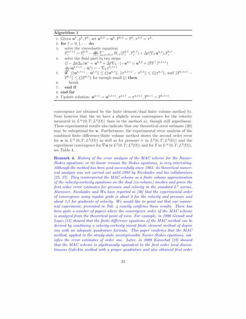
Algorithm 1

1: Given uk, pk,Fk, set uk,0 = uk,Fk,0 = Fk, πk,0 = πk.2: for ` = 0, 1, · · · do

3: solve the viscoelastic equation:Fk,`+1i = F

k,0i − ∆t

|Ti|

∑

j∈S(i) Hi j(Fk,`i ,Fk,`

j ) + ∆t(∇huk,`)iF

k,`i

4: solve the fluid part in two steps:(I−∆t∆h)u

∗ = uk,0 +∆t∇h · (−uk,l ⊗ uk,l + (FF>)k,`+1)1∆t(u

k,`+1 − u∗) = −∇hπk,`+1

5: if (‖uk,`+1 − uk,`‖ ≤ ξ‖uk,`‖, ‖πk,`+1 − πk,`‖ ≤ ξ‖πk,`‖, and ‖Fk,`+1 −Fk,`‖ ≤ ξ‖Fk,`‖ for enough small ξ) then

6: break7: end if

8: end for

9: Update solution: uk+1 = uk,`+1, πk+1 = πk,`+1,Fk+1 = Fk,`+1.

convergence are obtained by the finite element/dual finite volume method b).Note however that the we have a slightly worse convergence for the velocitymeasured in L∞(0, T ;L2(Ω)) than in the method a), though still superlinear.These experimental results also indicate that our theoretical error estimate (20)may be suboptimal for u. Furthermore, the experimental error analysis of thecombined finite difference/finite volume method shows the second order errorfor u in L∞(0, T ;L2(Ω)) as well as for pressure π in L2(0, T ;L2(Ω)) and thesuperlinear convergence for ∇u in L2(0, T ;L2(Ω)) and for F in L∞(0, T ;L2(Ω)),see Table 4.

Remark 4. History of the error analysis of the MAC scheme for the Navier-Stokes equations, or its linear version the Stokes equations, is very interesting.Although the method has been used successfully since 1965, its theoretical numer-ical analysis was not carried out until 1992 by Nicolaides and his collaborators[25, 27]. They reinterpreted the MAC scheme as a finite volume approximationof the velocity-vorticity equations on the dual (co-volume) meshes and prove thefirst order error estimates for pressure and velocity in the standard L2 norms.Moreover, Nicolaides and Wu have reported in [26] that the experimental orderof convergence using regular grids is about 2 for the velocity and pressure andabout 1,5 for gradients of velocity. We would like to point out that our numer-ical experiment, presented in Tab. 4 exactly confirms these results. There hasbeen quite a number of papers where the convergence order of the MAC schemeis analyzed from the theoretical point of view. For example, in 1996 Girault andLopez [15] showed that the finite difference equations of the MAC method can bederived by combining a velocity-vorticity mixed finite element method of degreeone with an adequate quadrature formula. This paper confirms that the MACmethod, applied to the steady-state incompressible Navier-Stokes equations, sat-isfies the error estimates of order one. Later, in 2008 Kanschat [19] showedthat the MAC scheme is algebraically equivalent to the first order local discon-tinuous Galerkin method with a proper quadrature and also obtained first order

23

convergence of the scheme. Further, in 2014 Herbin et al. [17] have shown theconvergence of the MAC scheme for the Navier-Stokes equations on non-uniformgrids. In [12] a related method, the so-called colocated finite volume scheme forthe Stokes problem is studied and its first order convergence is proven theoreti-cally. Here it is also reported that the second order convergence for velocity isobtained in numerical experiments.

Nevertheless, until very recently the superconvergence of the MAC schemehas not been confirmed theoretically. In 2014 Li and Sun [22] succeeded to showthe second order convergence of velocity and pressure measured in the L2 normseven for irregular rectangular grids. The authors do not reinterpret the MACmethod as the finite volume or finite element scheme, but work directly in thefinite difference framework. Careful and elegant analysis of various sources oferrors shows that although the local truncation errors are only first order, a suit-able cancelation of local errors yields after summation the second order globalerrors for both velocity and pressure. Our numerical experiments presented inTable 4 for the combined finite difference/finite volume method confirm theoret-ical results of Li and Sun. As a consequence the velocity gradients ∇u as wellas the deformation gradient F converge superlinearly with the order 1,5.

In what follows we present graphs of the solution at the final time T = 0.2.In Figure 2 we plot the streamlines, pressure and velocity components. Figure 3presents all components of the deformation gradient F. Further, Figure 4 illus-trates time evolution of the kinetic energy 1

2u2 and the L∞-norm of trace of the

stress tensor FF>. Although the kinetic energy is bounded, we see clearly thatL∞-norm of the stress tensor is not bounded.

0 0.2 0.4 0.6 0.8 10

0.1

0.2

0.3

0.4

0.5

0.6

0.7

0.8

0.9

1

0.1 0.2 0.3 0.4 0.5 0.6 0.7 0.8 0.9

0.1

0.2

0.3

0.4

0.5

0.6

0.7

0.8

0.9

−6

−4

−2

0

2

4

6

020

4060

80

0

20

40

60

80−1

−0.5

0

0.5

direction xdirection y

U

−1

−0.8

−0.6

−0.4

−0.2

0

020

4060

80

0

20

40

60

80−0.4

−0.2

0

0.2

0.4

direction xdirection y

V

−0.2

−0.15

−0.1

−0.05

0

0.05

0.1

0.15

0.2

Figure 2: Graph of the solution at the final time T = 0.2: streamline (top left),pressure (top right) and velocity components u1 and u2 (bottom).

24

Conclusions

In this paper we have studied a particular variant of the Oldroyd-B visocelasticmodel having the limiting relaxation time going to infinity. Assuming globalin time existence of enough regular weak solution we have studied the errorestimates of a standard finite element method A and of a combined finite ele-ment/dual finite volume method B. Main theoretical result Theorem 1 shows thefirst order error estimates for a standard finite element discretization using theTaylor-Hood elements for the velocities and pressures and the linear elementsfor the deformation gradient F. These results are also confirmed by a numberof numerical experiments, a representative choice is presented in this paper.Furthermore, our theoretical results indicate the errors of order O(h3/4) for thecombined finite element/dual finite volume method. Numerical experiments forthe above two methods confirm our theoretical results. Moreover, using thefinite difference/finite volume approximation on a rectangular grid, we get eventhe second order convergence of the velocity u and of pressure π, which is a con-sequence of the superconvergence of the special finite-difference approximationof the Navier-Stokes equations. Using the recent theoretical results of Li andSun [22] it would be interesting to study theoretically also the convergence ofthe combined finite difference/finite volume scheme for our viscoelastic modelin future.

Acknowledgement. H.M., B.S. and M.L-M. were supported by the GermanScience Foundation under the grant IRTG 1529 “Mathematical Fluid Dynam-ics”. J.S. was supported by the Czech Science Foundation grant no. P 201/11/1304in the general framework of RVO: 67985840. B.S. and H.M. would like to thankProfs. Tabata and Notsu (Waseda University, Tokyo) for fruitful discussions onthe topic.

References

[1] J. Barrett and S. Boyaval. Existence and approximation of a (regularized)Oldroyd-B model. Math. Models Methods Appl. Sci., 21:1783–1837, 2011.

[2] S. Boyaval, T. Lelievre, and C. Mangoubi. Free-energy-dissipative schemesfor the Oldroyd-B model. Mathematical Modelling and Numerical Analysis,43:523–561, 2009.

[3] S. C. Brenner and R. Scott. The mathematical theory of finite elementmethods, volume 15. Springer, 2008.

[4] F. Brezzi and M. Fortin. Mixed and hybrid finite element methods. Springer,1991.

[5] X. Chen, H. Marschall, M. Schfer, and D. Bothe. A comparison of sta-bilisation approaches for finite-volume simulation of viscoelastic fluid flow.Int. J. Comput. Fluid Dyn., 27(6-7):229–250, 2013.

25

[6] Y. Chen and P. Zhang. The global existence of small solutions to the in-compressible viscoelastic fluid system in 2 and 3 space dimensions. Comm.Partial Differential Equations, 31(10-12):1793–1810, 2006.

[7] P. Constantin and M. Kliegl. Note on global regularity for two-dimensionalOldroyd-B fluids with diffusive stress. Arch. Ration. Mech. Anal., 206(3):725–740, 2012.

[8] P. Constantin and W. Sun. Remarks on Oldroyd-B and related complexfluid models. Commun. Math. Sci., 10(1):33–73, 2012.

[9] B. Daly, F. Harlow, J. Shannon, and W. J.E. The MAC method. Technicalreport LA-3425, Los Alamos Scientific Laboratory, University of California,1965.

[10] H. Damanik, J. Hron, A. Ouazzi, and S. Turek. A monolithic FEM ap-proach for the log-conformation reformulation (LCR) of viscoelastic flowproblems. J . Non-Newton. Fluid Mech., 165:1105–1113, 2010.

[11] V. Dolejsı, M. Feistauer, and C. Schwab. A finite volume discontinuousGalerkin scheme for nonlinear convection–diffusion problems. Calcolo, 39(1):1–40, 2002.

[12] R. Eymard, R. Herbin, and J. C. Latche. On a stabilized colocated finitevolume scheme for the Stokes problem. M2AN Math. Model. Numer. Anal.,40(3):501–527, 2006.

[13] R. Fattal and R. Kupferman. Time-dependent simulation of viscoelasticflows at high Weissenberg number using the log-conformation representa-tion. J . Non-Newton. Fluid Mech., 126:23–37, 2005.

[14] E. Fernandez-Cara, E. Guillen, and R. Ortega. Mathematical modeling andanalysis of viscoelastic fluids of the Oldroyd kind. In Handbook of NumericalAnalysis, Vol. VIII, pages 543–661. North-Holland, Amsterdam, 2002.

[15] V. Girault and H. Lopez. Finite-element error estimates for the MACscheme. IMA J. Numer. Anal., 16(3):247–379, 1996.

[16] C. Guillope and J. Saut. Global existence and one-dimensional nonlinearstability of shearing motions of viscoelastic fluids of Oldroyd type. RAIROModelisation Math. Anal. Numer., 24:369–401, 1990.

[17] R. Herbin, J.-C. Latche, and K. Mallem. Convergence of the MAC schemefor the steady-state incompressible Navier-Stokes equations on non-uniformgrids. In Finite volumes for complex applications. VII. Methods and the-oretical aspects, volume 77 of Springer Proc. Math. Stat., pages 343–351.Springer, Cham, 2014.

[18] M. Hieber, Y. Naito, and Y. Shibata. Global existence results for Oldroyd-B fluids in exterior domains. J. Differential Equations, 252(3):2617–2629,2012.

26

[19] G. Kanschat. Divergence-free discontinuous Galerkin schemes for theStokes equations and the MAC scheme. Internat. J. Numer. Methods Flu-ids, 56(7):941–950, 2008.

[20] O. Kreml and M. Pokorny. On the local strong solutions for a systemdescribing the flow of a viscoelastic fluid. Banach Center Publ. v86, pages195–206, 2009.

[21] V. Lebedev. Difference analogoues of orthogonal decompositions, funda-mental differential operators and certain boundary-value problems of math-ematical physics. Z. Vycisl. Mat. i Mat. Fiz. (in Russian), 4:449–465, 1964.

[22] J. Li and S. Sun. The superconvergence phenomenon and proof of theMAC scheme for the Stokes equations on non-uniform rectangular meshes.J. Sci. Comput, DOI 10.1007/s10915-014-9963-5, 2014.

[23] F.-H. Lin, C. Liu, and P. Zhang. On hydrodynamics of viscoelastic fluids.Comm. Pure Appl. Math., 58(11):1437–1471, 2005.

[24] P.-L. Lions and N. Masmoudi. Global solutions for some Oldroyd modelsof non-Newtonian flows. Chin.Ann. Math., Ser. B, 21(2):131–146, 2000.

[25] R. A. Nicolaides. Analysis and convergence of the MAC scheme. I. Thelinear problem. SIAM J. Numer. Anal., 29(6):1579–1591, 1992.

[26] R. A. Nicolaides and X. Wu. Numerical solution of the hamel prob-lem by a covolume method. Advances in Computational Fluid Dynamics,(W.G. Habashi and M. Hafez,eds.):397–422, 1995.

[27] R. A. Nicolaides and X. Wu. Analysis and convergence of the MAC scheme.II. Navier-Stokes equations. Math. Comp., 65(213):29–44, 1996.

27

0 0.2 0.4 0.6 0.8 10

0.1

0.2

0.3

0.4

0.5

0.6

0.7

0.8

0.9

1

0.7

0.8

0.9

1

1.1

1.2

1.3

1.4

1.5

0 0.2 0.4 0.6 0.8 10

0.1

0.2

0.3

0.4

0.5

0.6

0.7

0.8

0.9

1

−1

−0.8

−0.6

−0.4

−0.2

0

0 0.2 0.4 0.6 0.8 10

0.1

0.2

0.3

0.4

0.5

0.6

0.7

0.8

0.9

1

−0.2

−0.15

−0.1

−0.05

0

0.05

0.1

0.15

0 0.2 0.4 0.6 0.8 10

0.1

0.2

0.3

0.4

0.5

0.6

0.7

0.8

0.9

1

0.7

0.8

0.9

1

1.1

1.2

1.3

1.4

1.5

1.6

Figure 3: Graph of the solution at the final time T = 0.2; four components ofthe deformation gradient Fij , i, j = 1, 2, from the top left to the bottom right.

0 0.05 0.1 0.15 0.22

2.1

2.2

2.3

2.4

2.5

2.6

2.7

2.8

2.9

3Re = 1

time

trac

e(F

FT)

0 0.05 0.1 0.15 0.20.004

0.006

0.008

0.01

0.012

0.014

0.016

0.018

0.02

0.022

time

kine

tic e

nerg

y

Figure 4: Time evolution of the maximum trace of the elastic stress tensor Te

(left) and of the kinetic energy (right).

28