An on-line turbulence profiler for the

VLT’s adaptive optics facility (AOF)

Andrés GuesalagaPontificia Universidad Católica de Chile

Visitor at Université Nice, Sophia-Antipolis, Feb. 2018

Staff

• 8 professors (permanent positions)

• 7 postdocs

• 14 graduate students

Centro de Astro-Ingeniería

Some research activities

• High resolution spectroscopy (Vanzi et al.)

Echelle spectrographs, Fibre optics characterization

• Planet finding (Jordán, Suc, et al.)

Hat-South member

• Cosmic microwave background (Dunner & Cactus group)

ACT (145, 220 and 280 GHz)

• Cosmological Simulations (Padilla et al.)

• Wide-field adaptive optics (Bechet, Guesalaga et al)Atmospheric Characterization, Vibrations Mitigation, Laser shaping

Teaching Observatory @ Sta. Martina

(outskirts of Santiago)

• Undergraduate teaching

• Testing of instruments

• ESO 50 cm, CTIO 40 cm

Laboratory equipment (Adaptive optics)

• 5 optical tables (1 MOAO experimental setup)

• 3 Boston MEMS DM, 140 actuators

• 1 Xinetics DM, 37 actuators

• 3 bimorph DMs, 48 actuators

• 5 Shack-Hartman WFS (24 x24 subapertures)

• Phase-screens for turbulence simulation

Centro de Astro-Ingeniería

Motivation for embedded profilers:

• An on-line profiler can help to characterize the performance of the AO system

• Predictive control via estimation of wind speed and wind direction

• Gather turbulence statistics of the site

• Characterization of the telescope environment (dome seeing, vibrations, mis-reg.)

• Optimize tomographic reconstructors and conjugation altitudes for DMs according

to Cn2 (h), L0(h), wind, dome seeing, etc.

“Embedded” (on-line) turbulence profilers(profilers using WFS of telescopes’ facility instruments)

WindflowoverdomeBoundarylayer

Tropopause

Stratosphere

~1Km

10-12Km

SLODAR using

AO WFS data

(García-Lorenzo &

Fuensalida, MNRAS,

2011

← 60 arcseconds →

0

1 2

5 4

• 16x16 grid Shack-Hartmann

• 204 active subapertures (total: 1020)

• sampling rate <= 800 Hz

5 WFSs

3 DMs• 917 actuators in total

• 684 valid actuators (seen by the WFSs)

• 233 extrapolated actuators

0 km 4.5 km 9 km

A Profiler for GeMS (Gemini-South MCAO System )

CANOPUS(The beginning)

For T = 0 s, the turbulence profile in altitude is extracted from the baseline

For T > 0, the layers present can be detected and their velocity estimated

w = 8.8 m/s

αw = 187.1°

w = 21.3 m/s

αw = 227.7°

GeMS: The Cn2(h) and “wind profiler”

Cortés et al, MNRAS, 2018

GeMS: statistics for 1000+ profiles(Several campaigns in 2012, 2013 and 2014)

0.05

0.1

0.15

0.2

0.25

0.3

r0 for run13

r0 [m

]

Run 13

hours

alt

itu

de

Profiles20Km

0Km

Histogram of r0Histogram of isoplanatic

angle, θ0

GeMS: statistics for 300+ L0(h) profiles(Several campaigns in 2012, 2013 and 2014)

High altitude wind direction, h>7Km

Wind direction (polar plot histogram )

Outer-Scale Profile

Guesalaga et al, MNRAS, 2017

Comparing GeMS wind profiles to Meso-NH model

Sivo et al, MNRAS, 2018

Red crosses are from GeMS profiler, continuous line is the meso-NH model

0 1 2 3 4 5 6 7 8 9

hours

Altitude, Km

20

16

12

8

4

0

Turbulence profile at Pachón, April 16th 2013

GeMS: frozen flow study

Wind speed = 21.3 m/s

Wind direction = 227.7°

Turbulence profiles at Pachón, April 16th 2013

Dependence of frozen flow to wind speed

GeMS: Frozen flow study

the slope is in m-1

Guesalaga et al, MNRAS, 2014

Problems with GeMS profiler

• Resolution in altitude limited by subaperture diameter.

• Strong effect of L0(h) on accuracy, specially for layers near the

ground or system operating under strong dome turbulence

conditions.

• When trying to isolate individual layers, there are multiple

functions to deconvolve the cross-correlation image (depending

on height and outer-scale), so it is not a practical approach.

• Long processing time (t > 7 mins).

Main conclusion: including L0(h) in every step of the

profiling process is a must.

An On-line Profiler for ESO’s Adaptive

Optics Facility (AOF)

AOF main characteristics:- 3 operational modes: GALACSI x 2 and GRAAL

- 4 sodium laser asterism

- WFSs: 40 x 40 subapertures (20cm diameter)

- Deformable secondary mirror (1170 actuators)

HR

HR

LRLR

Colaborators from ESO: J.Kolb, S.Oberti, J.Valenzuela

An On-line Profiler for ESO’s Adaptive

Optics Facility (AOF)

GRAAL feeds HAWK-I, a NIR imager (0.85 - 2.5 µm). The science field of view is

7.5 arcmin square. GRAAL compensates for the lowest layers of the atmospheric

turbulence (up to ~ 2 km.

GALACSI is the AO system developed to increase the performance of the

MUSE instrument, a panoramic integral-field spectrograph working at visible

wavelength.

ESO’s Adaptive Optics Facility (AOF)

AOF main characteristics:

- 4 sodium laser asterism

- WFSs: 40 x 40 subapertures, 20cm diameter

- 2 altitude resolutions (star separations)

- Deformable mirror for GLAO and LTAO

- 3 operational modes: GALACSI x 2 and GRAAL

HR

HR

LRLR

Range is due to the

LGS cone effect

The method: Cross-Correlations of Pseudo Open Loop

Slopes (POLS) for pairs of WFSs

HR

HR

LRLR

Notice that turbulence

on the edge of WFS1-2

is out of the detectable

región of WFS2-4

The method: Reference or response functions

The first step in the profiling technique is to generate (only once) the reference functions: cross-

correlations between pairs of WFSs POLS for different values of layer height and outer scales.

A grid of 33 altitude divisions and 12 outer-scale values is constructed

• Discrete values for L0 : {1, 2, 3, 4, 6, 8, 11, 16, 22, 32, 50, 100}

• Discrete values for h : {1:N}·Δh, N is chosen ≈ 80% of maximum number of bins

asymmetric

shapes

Guesalaga et al, MNRAS, 2017

The method: Search for minimum using interpolated

functions from reference grid

Reference

functions

Interpolated

function

),(),()1(

)1(),(),()1(),(

11

0

1

0

1

000

ji

ref

ji

ref

ji

ref

ji

refref

hChC

hChChC

LL

LLL

2

1

0,,

),(0

ZN

i

i

refimeash

hCCMin LL

Search for mínimum:

Interpolation:

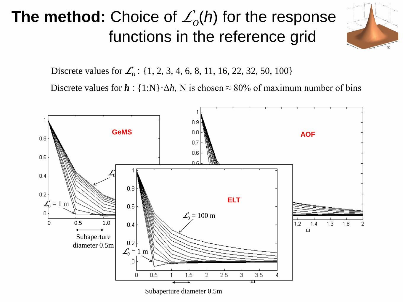
Discrete values for L0 : {1, 2, 3, 4, 6, 8, 11, 16, 22, 32, 50, 100}

The method: Choice of L0(h) for the response

functions in the reference grid

L0 = 100 m

L0 = 1 m

0 0.5 1.0 1.5 2.0m

GeMS

Subaperture

diameter 0.5m

L0 = 100 m

L0 = 1 m m

AOF

Subaperture

diameter 0.2m

Discrete values for h : {1:N}·Δh, N is chosen ≈ 80% of maximum number of bins

For an 8m telescope, measuringL0 above 32m is unreliable

L0 = 100 m

L0 = 1 m

m

ELT

Subaperture diameter 0.5m

4 layers 5 layers

1 layer 2 layers 3 layers

3D

measured

fitted

error

8 layers

final fitting

error

The method: Fitting sequence

Unsensed

turbulence

Maximum probed height

for GALACSI WFM

Mode:

GALACSI - WFM

The method: Fitting sequence

The method: Temporal Cross-Correlation (wind speed)

Comparison against an independent

technique for seeing and global L0

seeing

Global outer-

scale

Seeing linear

regression

SeeingESO =

= 0.92SeeingPUC + 0.06

Mode: GRAAL

Implementation in SPARTA (AOF’s RTC)

Mode: GALACSI - NFM

Conclusions for turbulence profiling

• The information exists for accurate profiling (in quantity and

quality)

• Profiles for Cn2, L0 and wind direction & magnitude are currently

in use in the AOF (automatic wind profiles under development)

• Including the outer scale in the profiling methods is a must

• In the ELT, the outer scale estimation will be essential

• Reliable estimation of larger outer scales is limited to 3 or 4

times the diameter of the telescope (30m for the VLT; 150m for

the ELT)

• Processing times compatible with system operation (t < 2 mins

@ 8 layers)

• A comprehensive comparison with simultaneous with Durham’s

Stereo-SCIDAR data is coming soon